the Creative Commons Attribution 4.0 License.
the Creative Commons Attribution 4.0 License.
 | 13 Jan 2023
Evolution of squall line variability and error growth in an ensemble of large eddy simulations
Holger Tost
A chain of processes is identified that regulates much of the spread in an ensemble of squall lines in large eddy simulations with tight initial conditions. Patterns of gravity wave propagation de-correlate and restructure the initial condition spread until a second phase of convective initiation is taking place, i.e. after 30 min of simulation time. Subsequently, variability in this convective initiation and mass overturn is associated with differences in cold pool propagation within the ensemble (propagation at 2–4 m s−1.
An ensemble sensitivity analysis reveals that anomalies in squall-line-relative flow with respect to the ensemble mean are also associated with the secondary convective initiation. Downdraughts are fed with extra air by a convergence zone on the rearward flank of the updraughts. An analysis of difference growth within the ensemble shows that a substantial proportion of variability is explained by cold pool propagation contrasts during this stage (30–80 min), which is partly removed when a feature-relative perspective is taken. The patterns of coherent variability exist on the timescale of an hour and dissipate subsequently (80–100 min).
- Article
(4795 KB) - Full-text XML
-
Supplement
(4539 KB) - BibTeX
- EndNote


Squall lines are complex meteorological phenomena consisting of an elongated linear area with convective cells that usually induce a coherent mesoscale circulation. They often develop into mixed stratiform–convective precipitation systems with spatial extents of up to several hundred kilometres in the horizontal and a lifetime exceeding several hours. Squall lines are an active research field for several decades (Houze, 2004, 2018). The goal of this study is to understand the dynamical processes that govern ensemble spread in large eddy simulations of idealised squall lines.
Due to the increasing computational resources, high-resolution simulations in convective studies have become feasible, nowadays. Throughout the last 25 years, simplified cloud-resolving kilometre-scale simulations (Weisman et al., 1997) could be extended to systematic sets of fully three-dimensional large eddy simulations (LESs) at high resolutions (Adams-Selin, 2020a, b). This allowed for an improved understanding of the impact of shear profiles and resulting convective organisation (e.g. Weisman and Rotunno, 2004; Coniglio et al., 2006; Adams-Selin, 2020a), including squall line organisation. While large eddy simulations of squall lines become increasingly attainable, contrasts in representation of increasingly small-scale processes between simulation pairs can be analysed: the model impact of resolution on squall line evolution and associated convergence at (sufficiently) high resolution (Weisman et al., 1997; Bryan et al., 2003; Lebo and Morrison, 2015). Bryan et al. (2003) found that even LESs do not result in true convergence of solutions, as the need for parameterising processes shifts to sub-grid turbulence in a partly represented inertial sub-range and microphysics. However, statistical (bulk property) convergence occurs already at coarser grid spacing, while local numerical convergence may not occur at all (Langhans et al., 2012). How squall lines can sensitively depend on microphysics, shear and instability has been investigated by, for example, Morrison et al. (2009); Grant et al. (2018); and Adams-Selin (2020a, b).
Squall line ensembles and their error growth have been investigated by Melhauser and Zhang (2012); Hanley et al. (2013); and Weyn and Durran (2017). Individual ensemble members were compared to each other with a focus on the differences in their evolution. Even though squall line development and sensitivity has been addressed in LES, e.g. Adams-Selin (2020a, b), error growth has not been addressed at sub-kilometre grid spacing, to the knowledge of the authors, but only at kilometre-scale convection-permitting resolution, e.g. by Weyn and Durran (2017). At LES resolutions (100–200 m), smaller-scale processes can be included in a process-based analysis: updraughts (Varble et al., 2020), cold pools (Grant et al., 2018) and gravity waves are represented explicitly, and their dynamics can be addressed directly, which is needed for improved understanding of small-scale error growth. Error growth studies at large scales suggest that deep convection is an important process to address in error growth studies (e.g. Selz et al., 2022; Baumgart et al., 2019; Rodwell et al., 2013).
Application of the word “error” and similar terms (“intrinsic limit”) to ensemble differences requires a perfect model assumption or a perfect error assumption (e.g. Selz, 2019): the physics of errors has to be assumed to be represented perfectly in a numerical model, which is reasonable at >7Δx but not at smaller scales (Skamarock, 2004). Melhauser and Zhang (2012) and Hanley et al. (2013) looked at simulations featuring a real squall line case in a local area model from the larger mesoscale and synoptic point of view. The squall line dominated the dynamical evolution of the regional atmosphere in both sensitivity studies, even though downscale “contamination” from the synoptic scale was considered. Melhauser and Zhang (2012) found that an intrinsic limit of predictability can affect a squall line ensemble: by reducing initial condition spread by a factor of 8, their simulations could diverge about as much without reduced initial condition spread. Furthermore, the contingency of convective initiation was a key process for the ensemble spread, a process of which the limited predictability would be expected to be driven by spatio-temporal variability at even smaller scales (Lorenz, 1969). Convective initiation was also found to be a key process by Hanley et al. (2013).
Weyn and Durran (2017) have looked at error growth in mesoscale convective systems with squall-line-like features in isolation. They used a grid spacing of 1 km on a domain with horizontal scales of about 500 km. The study mostly analysed error growth from the spectral point of view, which implies that there was much less attention on convective and accompanying processes in physical space. They have compared the error growth of divergent and rotational wind components and found that divergent winds are mostly affecting larger-scale errors. Furthermore, an important finding was that by reducing initial condition spread by factors of 5 and 25, only about 1 h of predictability was gained, which is hardly significant compared to their error saturation timescale of about 5 h.
In this study, sensitivity is analysed from a dynamical point of view with squall line simulations in isolation from a synoptic and larger mesoscale environment. Error growth is analysed in high-resolution simulations (200 m) with 10 ensemble members. The dynamical aspects that are analysed are the following, including a short review for each of them:
-
Gravity wave dynamics. Interaction between gravity waves and a convective environment has been investigated using a linear gravity wave model (Bretherton and Smolarkiewicz, 1989; Nicholls et al., 1991; Mapes, 1993). A convective system is mimicked by a latent heating source in these papers. Subsequently, cloud models have been used to address the concentration of localised upward motion by gravity waves, with several vertical gravity wave modes favouring certain regions of convective initiation that lead to coherent patterns and upscale organisation (e.g. Lane and Reeder, 2001; Stechmann and Majda, 2009; Adams-Selin and Johnson, 2013; Lane and Zhang, 2011; Grant et al., 2018, and references in the latter two). In addition, Bierdel et al. (2017) have created a model to study the error propagation from convective scales to large mesoscales and (sub-)synoptic scales caused by differences in convective heating based on the linear gravity wave model (Bretherton and Smolarkiewicz, 1989; Nicholls et al., 1991). However, they focused on scales substantially larger than (sub-)squall line scales investigated here.
-
Convective initiation. Fovell et al. (2006) showed how gravity waves affect squall line regions on smaller scales from the convective initiation point of view. In their simulations with explicitly resolved deep convection, it was shown how gravity waves can initiate discrete convective cells ahead of a squall line, which can merge with the main system. A sensitivity of these discrete convective cell was identified, which leads to a diverging evolution as a result of contrasts in convective initiation depending on the radiation treatment. The sensitivity of convective initiation has played an important role in Melhauser and Zhang (2012) and Adams-Selin (2020a, b), and it can nowadays be resolved more accurately due to finer grid spacing.
-
Cold-pool-relative motion or more specifically u in x–z plane averaged along squall lines. Pandya and Durran (1996) have looked at the (sub-)system-scale variability explained by thermally forced gravity waves and found that the mesoscale squall line circulation strongly depends on the magnitude and shape of thermal forcing. Low-level features, notably the rear inflow jet, depend on the low-level conditions, especially N2. Their study focused on the squall line circulation (u) in the plane perpendicular to the squall line orientation, and it also assessed the impact of modified physical processes on that flow.
-
Updraught and downdraught motion. Updraught and downdraught characteristics can be sensitive to resolution, possibly leading to biases in updraughts (or downdraughts) in a comparison to radar images (e.g. Varble et al., 2020; Lebo and Morrison, 2015; Varble et al., 2014), which could, for example, propagate to differences in momentum and buoyancy transport (Varble et al., 2020, 2014). However, since no comparison between simulations at different resolutions or observations and simulations is made here, such sensitivities are not studied. Furthermore, the grid spacing is believed to be fine enough for accurately resolving updraught and downdraught characteristics (Bryan et al., 2003; Lebo and Morrison, 2015; Varble et al., 2020).
This study is restricted to the analysis of one idealised squall line case with weak ensemble perturbations. Furthermore, the squall line evolution is initially nearly two-dimensional due to the nearly 2D flow and initial conditions. However, this nearly 2D structure is of benefit for the analysis of squall-line-relative flow. Considering a single case allows for detailed analysis of the dynamical aspects listed. The magnitude of applied ensemble perturbations are equivalent to a vertical wind profile uncertainty of about or less than one model layer in typical convection-permitting models. Altogether, the aim is to get a comprehensive overview of the processes in which errors (i.e. ensemble spread) are showing up in a high-resolution squall line ensemble, following the evolution of small initial perturbations. We also describe how these errors may be transferred from one process to another. Furthermore, intrinsic predictability can be addressed, given the small magnitude of initial condition perturbations. Zonal shear in a shallow layer is perturbed randomly with magnitudes of 0 %–5 %, as opposed to the often used systematic approaches (e.g. Selz, 2019; Zhang et al., 2019; Selz et al., 2022; Melhauser and Zhang, 2012).
Analysis techniques are applied which are not so commonly used in studies of mesoscale convective systems. Next, more widely used passive tracers (e.g. Grant et al., 2018), an ensemble sensitivity analysis (Hanley et al., 2013; Torn and Romine, 2015; Bednarczyk and Ancell, 2015, but the latter with parameterised convection) and a difference kinetic energy metric are used. Passive tracers are an important tool to identify variability in convective transport; by targeting at an inflow layer, contrasts can be identified early on. Thereby, variability in a secondary phase of convective initiation is revealed. In combination with a tailored ensemble sensitivity analysis to connect the strength of the convective initiation with subsequent evolution of the squall line circulation (u), the temporal evolution of effects of this phase of initiation is followed. System-relative flow and its relation with secondary convective initiation is analysed. The difference kinetic energy error growth metric and diagnostics provide further insights into the evolution of system-relative motion and its role in error growth (Zhang, 2005; Zhang et al., 2007).
In Sect. 2 the characteristics of the simulations are documented, as well as the initial conditions and ensemble design. Furthermore, the spatio-temporal focus of our analysis is defined, and the statistical verification techniques are described. In Sect. 3 the main analysis is carried out, preceded by a description of diagnostics used in a subsection. The section starts with a general evolution of the simulated squall line echoes. After looking at the simulated radar reflectivities, the comparison section (Sect. 3.2) describes secondary convective initiation and identifies a relation with gravity wave signals. This is followed by an investigation of the cold pool propagation (Sect. 3.3.1). Then ensemble sensitivity analysis (Sect. 3.3.2) assesses the connection with the squall-line-relative flow, followed by an investigation of downdraughts and additional statistical considerations (Sect. 3.3.3). Section 3 ends with an error growth (Sect. 3.4) analysis in grid point space and a system-relative flow framework to highlight associated contrasts in error growth. The set of analyses is synthesised in Sect. 4, followed by a discussion (also in that section). This discussion leads to the conclusions, as given in Sect. 5.
2.1 Model configuration
Experiments are conducted with the cloud-resolving model CM1 (version 19.8) on a 120 by 120 km grid with a depth of 20 km and duration of 2 h simulation time, using the model version of Bryan (2019). The time steps are 0.75 s, with output stored every 5 min. The grid has a 200 m horizontal grid spacing and 100 m vertical grid spacing. The upper 5 km of the domain consists of a sponge layer with damping that absorbs upward-propagating gravity wave signals.
CM1 is running in large eddy simulation mode, where the sub-grid turbulence model is handled with a turbulent kinetic energy (TKE) scheme (Deardorff, 1980). The default CM1 microphysics scheme is used, which is the two-moment Morrison scheme with hail (Morrison et al., 2009), namely its version 3.6 – with resolved supersaturation and condensation based on saturation adjustment (see also Morrison et al., 2005). The advection scheme applies a fifth-order advection algorithm, and Coriolis acceleration is ignored. Radiation is not actively resolved, and no background tendencies have been set for radiation. All simulations use the same aforementioned settings.
The boundary conditions are non-periodic in all directions, leading to the availability of an infinite reservoir of inflow air. Derivatives of all quantities are set to 0 at the boundaries. Wave signals can therefore partially reflect at the boundaries. To reduce effects of boundary reflections, the outer regions on the north and south ends of the squall line are excluded from the main analysis framework. Details and download instructions for the namelist file and output data of all simulations can be found in the set-up and namelist material at https://tinyurl.com/groot-tost-22 (last access: 10 January 2023) (Groot, 2022).
2.2 Environmental conditions and ensemble perturbations
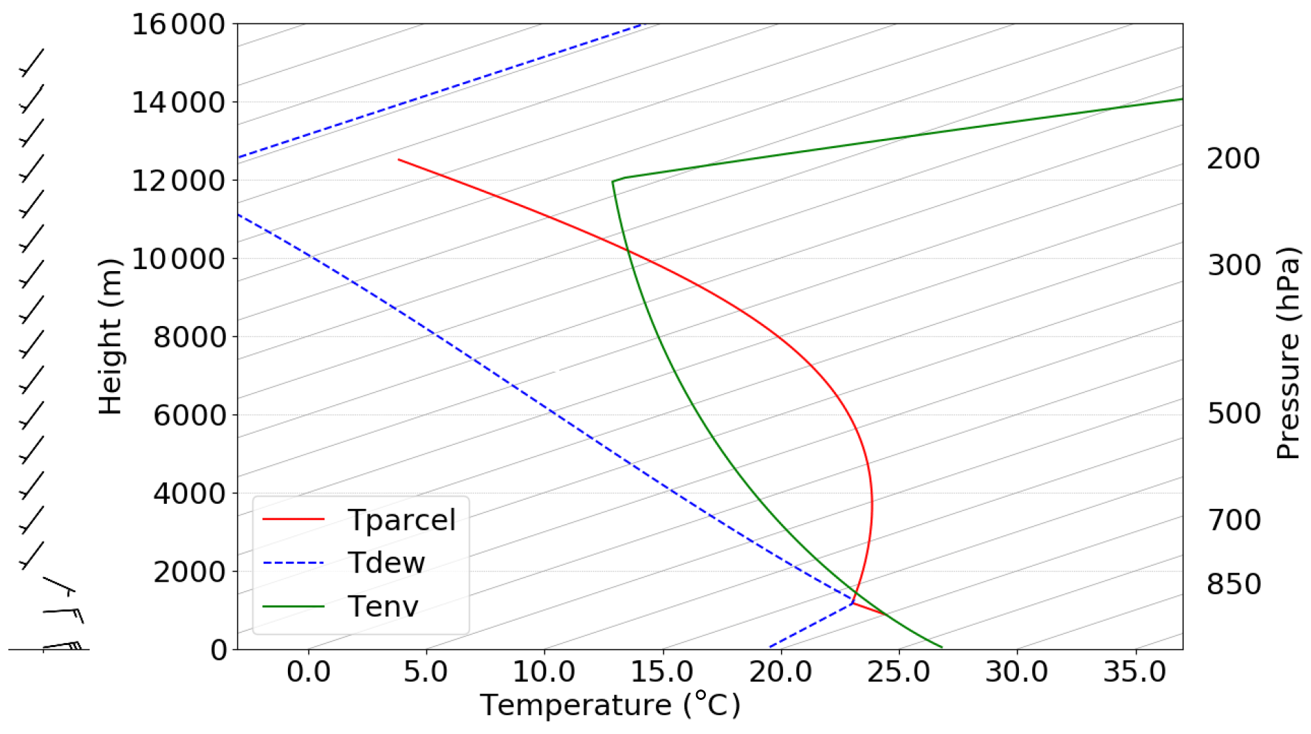
Figure 1Thermodynamical profile based on Weisman and Klemp (1982) and wind profile after Rotunno et al. (1988), with adjustments. Temperature: solid green line; dew point: dashed blue line; convectively lifted undiluted parcel's temperature: red line. The parcel is initially lifted from the mixed layer (at z=900 m).
The thermodynamic profile in each of the simulations is based on Weisman and Klemp (1982) (Fig. 1), which represents the conditions in the eastern half of the domain at t=0 min.
Below z=2500 m, a potential temperature perturbation that decreases linearly in magnitude with z from −6 K at the surface to 0 at 2500 m is set initially for the western half of the domain, x<0 km. The contrast between these two air masses triggers upward motion at their interface (x=0 km), and the given environment leads to a convectively very unstable environment (convective available potential energy, CAPE, of about 2000 J kg−1) for rising warm air mass in the east.
These environmental conditions of the Weisman and Klemp (1982) sounding are selected on purpose: the aim of this study is to analyse the behaviour of the ensemble spread of a squall line (when the development of a squall line is given) through the development of small deviations within the squall line. This perspective complements that of Melhauser and Zhang (2012), in which the sensitive dependence of a squall line is explored, including the critical dependence on primary convective initiation itself.
The basic character of the wind profile is adjusted from Rotunno et al. (1988), with the u component linearly varying from 12.5 m s−1 easterly inflow at the surface to westerly flow of 1.5 m s−1 above the top of the shear layer (Fig. 1). This top of the shear layer is set at m for the reference simulation. The v component of the wind varies linearly from −2 (surface) to +2 m s−1 (z≥zi) over the same layer. The latter is needed to develop three dimensionality in the simulation. Given fully 2D initial conditions, the three dimensionality could have been absent without any differential meridional advection in combination with the open boundary conditions (and no other small-scale perturbation sources, like random noise). Given that wind profile, the shear vectors are nearly perpendicular to the initial cold pool boundary. In combination with the strong convective instability near the interface, it leads to the formation of a squall line.
Note that deeper shear is omitted with the selected profile, which on average reduces the depth of vertical displacements and the size of convective systems (Coniglio et al., 2006). This is beneficial for a reduction of the storm-relative flow and hence to reduce the across-line growth of the squall lines: their residence time within the domain is increased.
An ensemble is generated by randomly perturbing the interface height (zi), with a maximum absolute deviation from the reference height zi,ref of −127 m (5 %) for ENS-05 zi,ENS-05 among the nine randomly drawn perturbed interface heights zi,ENS-X and a mean absolute deviation of 67 m (2.7 %) from zi,ref (see also Groot, 2022). These perturbed interface heights are then translated to the equivalent zonal and meridional velocities by linear interpolation below the perturbed interface and constant winds above at the model grid (vertically equidistant at 100 m intervals) to obtain the final perturbations. The magnitude of perturbations is equivalent to about one model level in high-resolution models; effectively, an extension or shrinkage of the sheared layer is achieved with these perturbations. However, the cold pool depth and hence the potential energy distribution is not affected by the ensemble perturbations; thus, only the initial kinetic energy distribution at low levels differs within the ensemble.
It is not given that variability imposed by initial shear perturbations within the ensemble is maintained until the formation of squall lines and beyond. Nonetheless, as a result of the 5 % variation in low-level shear intensity, systematic variability of nearly the corresponding magnitude in net latent heating may be anticipated: this would occur as a consequence of variability in layered overturning if the variability maintains itself (based on arguments by Coniglio et al., 2006; Alfaro, 2017).
2.3 Spatial and temporal windows for diagnostics
Diagnostics are applied to a central portion of the squall line region, where 40 km km to reduce the effects of the boundaries and their wave reflections on the analysis of the squall line evolution. Generally, boundary effects in the central part of the domain only become notable during the last 30–40 min of the simulation. The boundary conditions are solely based on the evolution of state variables at the domain edge, with the first derivatives set to zero right at the boundary. The evolution of state variables at the boundary is therefore different among ensemble members, even though the same type of boundary conditions is applied. These conditions are initially inherited by zi as much as their whole difference evolution to the reference simulation is controlled by the initial value of zi. In the x direction, a region within 1 km of the boundaries is excluded from the analysis.
Some analyses (ensemble sensitivity analysis in Sect. 3.3.2 and the error growth analysis of Sect. 3.4) are carried out relative to the cold pool edge, of which the detection is described later (in Sect. 3.3.1).
This study focuses on the evolution of the simulations up to 75–80 min. Nevertheless, the last 40 min of simulation time are also taken into account.
2.4 Statistical assessment of the robustness of signals
As an ensemble sensitivity analysis is used to investigate spatio-temporal variability in this study, a statistical criterion has been defined to evaluate if test statistics are globally significant to complement grid-point-based significance tests. To determine the robustness of the analysed signals given the small ensemble size (n=10), a statistical test criterion based on a t test has been defined. With the given ensemble size, correlation coefficients exceeding are significant at α of 0.05. That means their frequency of occurrence in any large random sample is expected to be about 5 % at p=0.05 and 1.25 % for random occurrence of (p=0.0125).
Statistical grid point testing is applied to spatial patterns within the squall line to determine a statistically significant signal: in case of a significant correlation of a feature of interest over a large fraction of the grid points located within its area, a pattern is considered significant. In the limit case this fraction f needs to theoretically fulfil a criterion close to f>2p (Wilks, 2016). On the contrary, other features without signals associated with it would simultaneously reveal small fractions of grid points with statistical significance. This is valid for most of the signals in the stratosphere (z of 15–20 km) for instance. If fully random, a significant area fraction f of about 0.05 is expected, with for p=0.05 and 0.025 for p=0.0125.
3.1 Evolution of squall line radar reflectivity
As an overview of the general properties of a squall line (one ensemble member with strong squall line development), the evolution of the simulated radar reflectivity is discussed. Reflectivity calculations in Morrison et al. (2009) are based on the assumption of Rayleigh scattering of 10 cm wavelength light by cloud ice, water and mixtures of those, integrating the water mass (Bryan, 2019).
3.1.1 Squall line evolution (one member example)
As a response to the (1) large latent instability, (2) relatively strong low-level wind shear perpendicular to the cold pool and the (3) strong forcing of upward motion by the cold pool, deep convection develops along the full length of the y axis. Narrow echoes of about 40 dBz right above the initial condition “discontinuity” at x=0 km appear after 15 min simulation time (Fig. 2a). About 5 to 10 min later, echoes exceeding 20 dBz reach above z=10 km, as can be deduced from Fig. 2c and d. Echoes also widen and exceed 60 dBz in the squall line core. Over the following 30 min, the squall line echoes grow monotonically at both anvil level and low/mid levels. The increase in areas with reflectivity >20 dBz occurs both upshear and downshear of the convective core (as could be deduced from Fig. 2g and h), which itself is close to stationary above x=0 km. However, the growth halts for a while on the downshear side after about 60 min and on the upshear side after about 75 min (Fig. 2k). Shrinkage of the areas with substantial cloud reflectivity occurs. After 80–90 min, stratiform precipitation develops on the upshear flank of the system (Fig. 2j), and the anvil expands in both directions towards the end of the simulation, growing to about 100 km length. However, the stratiform precipitation remains restricted to a limited region at the rear flank (Fig. 2j, at 3 km), and precipitation intensities remain rather low.

Figure 2Evolution of simulated reflectivity for ensemble member 3 and the reference simulation (only t=50 min) at z=3 km. A horizontal cross section is followed by corresponding x–z cross section directly below, with median reflectivity along the squall line. Left top (a, c): t=15 min, right top (b, d): t=25 min, left centre (e, g): t=50 min (ensemble member 3), right centre (f, h) t=50 min (reference simulation), left bottom (i, k): t=75 min, right bottom (j, l): t=100 min.
With initial conditions that depend on x and z but not on y, the system is nearly homogeneous in y initially (see Fig. 2), developing into a 3D squall line gradually. Gradients develop along the y axis with cells of higher reflectivity embedded within the line after 50 min and beyond. However, we will focus on results averaged in the y direction, as contrasts are largest in x and z directions and tend to be smoother and/or occur at smaller scales along the y axis.
3.1.2 Secondary phase of convective initiation
The evolution of the squall line in ensemble member 3 (ENS-03) is shown in Fig. 2. This member is at the very active end of the ensemble distribution. Within the first 30 min of the simulations, ensemble variability is barely detectable.
Upon this mature stage of the first line of cells follows a phase with secondary initiation (t=30 to 40 min). This secondary phase of convective initiation is most distinctive in ensemble member 3, where a secondary line of cells is triggered just ahead of the former line of cells and leads to forward displacements of the squall line core. The reflectivity pattern at t=50 min illustrates the forward displacement of convective cells and an increased area of reflectivity >55 dBz on the forward flank when the evolution of ensemble member 3 (ENS-03; Fig. 2e) is compared with the reference run (Fig. 2f). The reference run is not supporting the secondary phase of initiation; hence, the squall line appears to be stagnant until t=50 min (Fig. 2f). If echoes in the reference simulation reach x>5 km, it is anvil precipitation with reflectivity that reaches about 40 dBz just below melting level locally (z=4 km), as opposed to newly initiated updraughts with reflectivities up to 55–65 dBz (Fig. 2).
Following upon the second phase of convective initiation, the squall line starts accelerating eastward, with the reflectivities over 45 dBz at z=3 km propagating to x=10 km after 75 min and almost x=15 km after 100 min (ENS-03). The line becomes increasingly inhomogeneous in the y direction and exceeds 45 dBz at z=3 km over a longitudinal stretch of 15–20 km during this period, with core reflectivity of 65 dBz, which is a consequence of the strong forcing and high CAPE setting.
3.2 Detailed comparison of two example simulations
This section compares the two ensemble members (mentioned above; ensemble member 3 with strong secondary initiation and the reference simulation; see also Fig. 2) located at opposite ends of the distributions in most diagnostics. The spatio-temporal evolution of convergence and divergence zones is described (Sect. 3.2.1). Their motion delineates the temporal evolution of sources and sinks of convective updraughts.
Passive tracers are analysed for inspection of the contrasts within the simulation pair (Sect. 3.2.2).
3.2.1 Convergence and divergence zones
Figure 3 shows Hovmöller-like diagrams of divergence (red colours) and convergence (blue colours) in the lower and upper troposphere. The upper panels shows that the low-level convergence zone accelerates eastward in both simulations after a nearly stagnant position in the first 30 min approximately, in agreement with the displacement of cells in the previous section (Sect. 3.1.1). After this stagnant stage, the following patterns indicate eastward acceleration of convergence and divergence zones:
-
In the reference simulation the convergence zone quickly accelerates to stationary eastward propagation of about 2.5 m s−1 in the following 45–50 min, whereas it is substantially faster in ensemble member 3, with ∼ 4.3 m s−1.
-
A weak acceleration of the divergence zone in the wake of the former zone occurs, most prominently in ENS-03.
-
Another stage of acceleration of this zone occurs at the end of the simulations (90–120 min, x=0 to 30 km). However, this occurs after the analysis window and might be an effect of differences in boundary reflections.
The low-level convergence zone displaces suddenly after 0.6 h (green oval, Fig. 3) in ensemble member 3 (which opposes reference simulation), with a double divergence zone in its wake and an increase in amplitude of the convergence directly after. In the reference simulation this event happens in a smoother way: without a strong increase in amplitude of the convergence. On the contrary, the convergence zone also jumps by several kilometres in ENS-03 as opposed to the reference simulation. The jumpy displacement and amplitude increase of the convergence zone in ENS-03 relates to the secondary initiation of cells ahead of the squall line core (Sect. 3.1.1). The lower panels of Fig. 3 reveal a nearly stagnant and slightly diffuse patch of upper tropospheric divergence at x≈0 km, co-located with the squall line core, of which propagation is restricted to t>60 min (ensemble member 3 only).
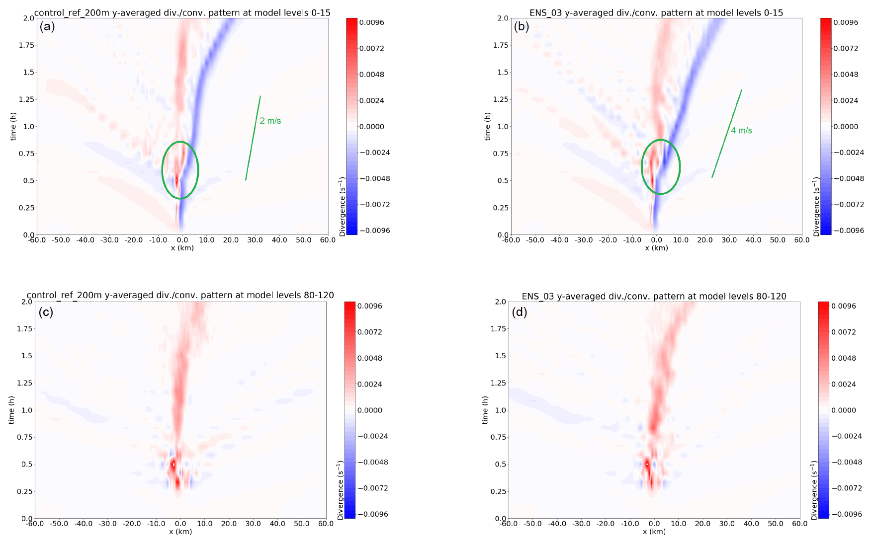
Figure 3Space–time distribution of low-level (0–1.5 km; a, b) and upper tropospheric (8–12 km; c, d) convergence (s−1) features in the reference simulation (a, c) and ensemble member 3 (b, d), averaged over all y and given z. A stage of particular interest that is analysed in the text is highlighted with a green oval, as well as the slope of the convergence zones halfway through the simulation.
3.2.2 Secondary convective initiation and tracers
Tracers are a tool to identify the convective circulation of air masses, as they provide quantitative information on the destination of specific inflow layers. The tool can be used to describe the circulation in the convective system, in a way comparable to a Lagrangian analysis. The tracer analysis is restricted to the identification of transport from their initialisation time until any output time and to a coherent air mass. In the simulations the tracers PT1 and PT2 are initiated below altitudes of 2.5 km ahead of the squall line. Consequently, the mixing of air masses at low levels there (and mainly the primary ascent) can be described, whereas the effect of rearward entrainment from mid-levels and their diluting effect can only be analysed with much more difficulty. Tracer PT1 was implemented below 800 m between x=0 and x=30 km at t=0, and PT2 was simultaneously initiated over the same horizontal region at all model levels where m. Concentrations are 0.001 kg kg−1 initially. These tracers are advected with the flow, with computations based on the advection scheme, but also the built-in sub-grid turbulence of the LES. No additional (e.g. microphysics-like) tendencies contribute to their redistribution.
In Fig. 4a the concentration of PT2 after 30 min is displayed for the two example simulations, the reference and ENS-03. Looking at the red shading (reference simulation), the tracer is transported towards negative x values as a result of westward flow at low levels, but it meets the updraught near x=0 km. It can be seen that the tracer initialised at levels about z=2 km has entered the updraught near x=0 km, and it has been transported upward by the updraught up to about z=10 km. Shifting the focus to the blue isolines (which represent ENS-03), mostly the same patterns are seen but with a slight westward shift of the updraught. Furthermore, while to the east PT2 concentrations in both of the simulations align nearly perfectly, a strong undulation is localised about 5 km to the east of the updraught in the PT2 pattern, when compared to the reference simulation. Therefore, the evolution of difference concentration after 25, 30 and 35 min is examined in the following.
The differences in PT2 concentrations between ENS-03 and the reference after 30 and 35 min are found in Fig. 4b, c and d. A surplus in PT2 is visible at the location of the black “X” in ENS-03 and a surplus about 1 km lower in the reference simulation after 30 min, amongst others.
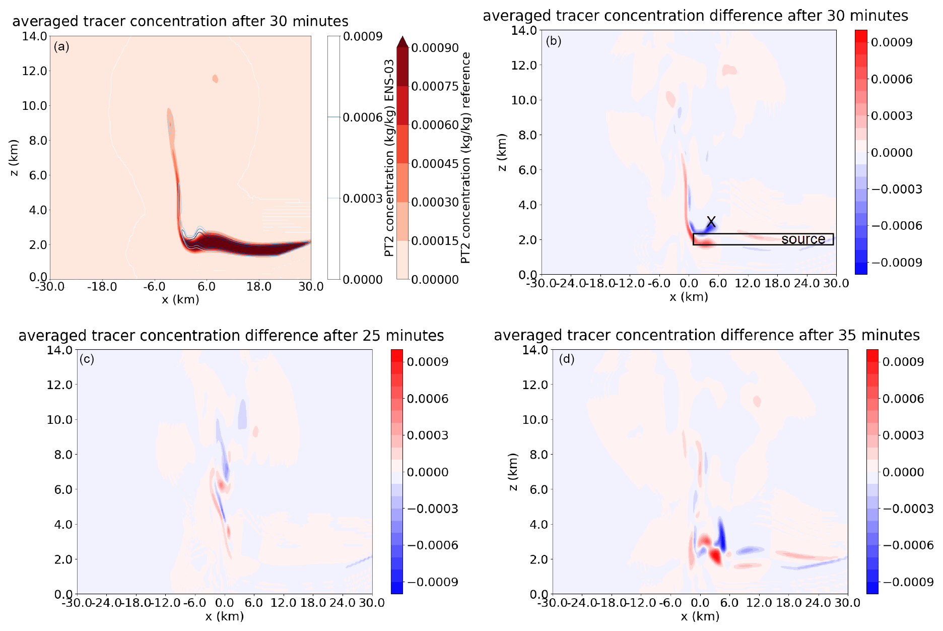
Figure 4PT2 concentration in reference (shading) and ENS-03 (isolines) and PT2 concentration difference between reference and ENS-03 (reference minus ENS-03) after 30 min (left, a, and right, b, at the top), 25 min (left bottom, c) and 35 min (right bottom, d). Red indicates a tracer surplus in reference simulation and blue in ENS-03. The black X (right, top, b) marks the gravity wave crest in which vertical displacement leads to triggering of a new line of convective cells in the squall line, as we will see later. Note that only half of the 120 km domain is shown.
A dipole structure in the PT2 surplus from z=4 km to z=6 km around x=0 km at t=25 min suggests a shift between the developing convective updraughts within the simulation pair in Fig. 4c. At t=30 min the dipole has elongated vertically: the updraught core is shifted eastward by a few grid cells in ENS-03 compared to the reference. Furthermore, the PT2 surplus at location X in ENS-03 is very notable. At this location, PT2 concentrations are much higher in ENS-03 than in the reference simulation at z=3 km, a few kilometres east of the x axis. About a kilometre below, PT2 concentrations are lower at the same time in ENS-03, at the lower flank of the source layer (Fig. 4b). A difference of opposite sign occurs at the top of (red; and below: blue) the PT2 source layer some 10 km to the east of X. After 35 min, the signal has propagated eastward by about 5–7 km, and the blue signal at location X has extended upward but the red has not.
Consequently, PT2 transport is substantially different between ensemble member 3 and the reference simulation (from t=30 to t=45 min): only 7.0 % of the PT2 mass moves from its low-level source layer to levels above 4 km height in these 15 min in the reference simulation, whereas 17.6 % does so in ensemble member 3. Furthermore, 11.7 % (ENS-03) is flowing to the upper troposphere (z>6 km) versus 6.0 % (reference simulation). This implies a large difference in convective tracer overturn; hence, convective mass fluxes are significantly larger in ensemble member 3 than in the reference simulation.
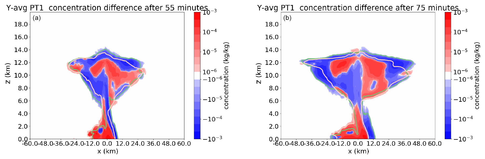
Figure 5Difference in PT1 concentration between ENS-03 (blue: higher) and reference (red: higher) after 55 min (a) and 75 min (b) in colours. In addition, the kg kg−1 isoline is shown for both simulations (salmon/bright pink colour: reference; green: ENS-03). The Y average is now taken over the limited sub-space, consisting of 40 km km.
Figure 5 displays the PT1 distribution after 55 and 75 min. The near-surface eastern boundary of PT1 moves faster eastward (in blue, ENS-03) than in the reference simulation (red). The near-surface eastern boundary corresponds with the location of the cold pool edge. Therefore, the relation between the identified tracer patterns is investigated further by looking at the cold pool displacement and the flow relative to the cold pool edge (Sects. 3.2 and 3.3.2). Additional patterns in PT1 are discussed in the Supplement.
3.2.3 Vertical velocity at X and interpretation
Location X in Fig. 4b has drawn our attention, with a contrast between upward and downward displacements of PT2 in the reference simulation and ENS-03. These downward/upward displacements in the trough/crest are resembling gravity wave patterns, as has been identified in the previous section. Furthermore, consequent differential vertical mass overturning has been identified with tracer evolution directly afterwards.
These identified patterns likely have a strong connection with vertical velocities at location X, which could be affected by both gravity wave variability first and then possibly by consequent variability in the potential for convective initiation, corresponding to the lifting of air above its LFC (level of free convection). The mean w along the squall line at location X (t=30 min) is +0.35 m s−1 in ENS-03 and −2.76 m s−1 in the reference, with along-line deviations of up to 1.5 m s−1 about the mean. Therefore, a large portion of line X along the squall line consists of locations favourable for convective initiation in ENS-03 with w>0, in contrast to the reference simulation in which w is well below 0 there. Other ensemble members are at intermediate values between the two opposites (mean w of −0.93 m s−1). Most members contain some limited areas favourable for the secondary convective initiation, as a result of the variability in w.
3.3 Ensemble squall line variability
The focus of the analysis is shifted towards the full ensemble, while variability within the highlighted ensemble pair in important squall line characteristics has been discussed. Key aspects are lag correlations of the cold pool edge with itself and the vertical velocity w at X (Fig. 4b). The relation of the latter with the meridionally averaged zonal cold-pool-relative flow (u) within the ensemble envelope is investigated. In the latter case, w of each ensemble member at location X acts as an independent variable. Additionally, other variables such as downdraught mass flux complement the holistic picture of the squall lines.
3.3.1 Location of the cold pool edge
The cold pool location and its time derivative, the propagation speed vcp, are computed at each output step by taking the maximum of at the lowest model level. This computation is done for each grid cell in the y direction. The cold pool position and velocity are obtained by taking the average value of the resulting x over y and converting this to a corresponding grid cell index. This way, a cold pool edge is defined as a function of ensemble member and time.
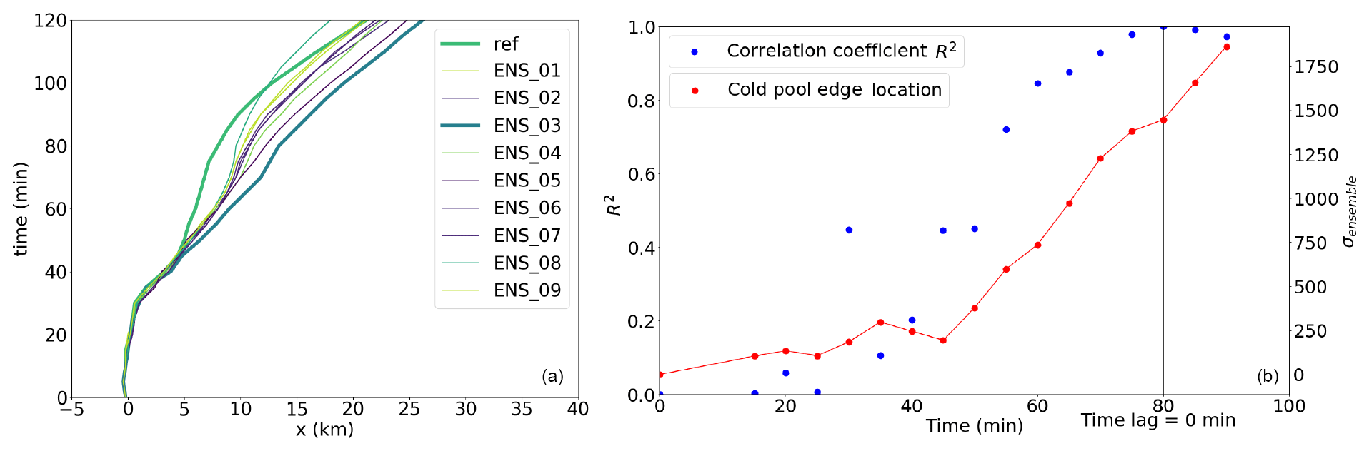
Figure 6(a) Hovmöller diagram of cold pool edge propagation, with colours in the order of their initial zi, with low interfaces in lime and high interfaces in purple (reference and ENS-03: bold). (b) R2 of time lag correlations as a function of simulation time (indicated) for the cold pool position among 10 ensemble members, with the position at t=80 min as reference correlation of 1 (blue; left y axis). Also shown is the temporal evolution of the standard deviation of the cold pool edge position in m (red; right y axis). The points at t=5 and 10 min are omitted, as there is no variability in cold pool edge location among the ensemble members (yet).
With this definition, vcp differs by a factor of 1.7 within the ensemble over the interval 30–75 min for the reference and ENS-03: 2.5 vs. 4.3 m s−1. That simulation pair only differs by 47 m in initial interface height of the shear layer (<2 %), while the two simulations are at the outer ends of the distribution of cold pool velocity!
The temporal evolution of the cold pool edge location is depicted in Fig. 6a, in which it is seen that a large contrast between the reference simulation and ENS-03 develops after about 45 min. Acceleration of the cold pools takes place after 30–40 min. The spread gradually develops after 45 min, with a kink in the propagation after about 80–100 min: towards further acceleration. The average displacement of the cold pool edge at the surface has been evaluated and lag correlated with its own location at t=80 min, i.e. directly at the point where the squall line effects start leaving the domain in the zonal direction.
The ensemble spread of the cold pool edge location is undetectable (up to one grid cell) during the squall line formation; consequentially and as a result of the small ensemble size, resulting lag correlations are frail. As the ensemble spread in the cold pool location increases to four grid cells after 40 min and increases linearly beyond, the sensitivity of lag correlations due to limited ensemble spread is substantially reduced and then eliminated. Consequently, beyond 30 min, the lag correlation provides insight into the ensemble spread.
Figure 6b depicts an S-like shape of the lag correlation. Roughly three stages can be distinguished. First, there is a stage prior to establishment of the intra-ensemble variability in cold pool location (not discussed further here – correlations are sensitive). Second, intra-ensemble variability of cold pool location is establishes in the next stage (35–50 min), corresponding with the growth stage of the S-curve. Here, the growth rate is maximised around 40–45 min. In the third stage, intra-ensemble variability has been established – starting at about 50–55 min – and is maintained until 80 min and beyond. In this stage, the cold pool locations have been set relative to each other: cold pools move jointly.
The ensemble variability structure is maintained. Both the standard deviation and the difference between maximum and minimum x of the cold pool edge increase nearly linearly beyond t=45 min (Fig. 6), which has also been suggested by Fig. 3 for ENS-03 and the reference.
3.3.2 Ensemble sensitivity analysis
The ensemble sensitivity technique is applied to assess patterns that exist in the squall line ensemble. The ensemble sensitivity finds the regression line through the dimension of the ensemble members that describes the best fit between two variables x1 and x2, like in any analysis of covariance patterns (see also Hanley et al., 2013; Bednarczyk and Ancell, 2015). Perturbations or excursions in an x2 with respect to an ensemble mean can be investigated in relation to those in variable x1. Furthermore, the temporal evolution of these perturbations of x2 can be followed, as structure within the ensemble envelope. The information of conditional variability in x2, conditional on x1, is revealed; hence, conditional coherent behaviour of a spatial-temporal flow pattern related to x1 later in time can be identified.
Bednarczyk and Ancell (2015) discuss limitations of this analysis for convective studies, which apply if the (spatial) extent of the independent variable is not exactly known and a proxy has to be used (as in their case): if deep convection is parameterised, precipitation or reflectivity-related output has to be analysed. On the contrary, the spatial extent of a variable of interest is clearly delineated for this case in Sect. 3.2.2 and Fig. 4 and it also points to the independent variable (local w).
Since squall line variability is investigated, the y-averaged variation in u in the x–z plane is of particular interest, especially within the squall line core. This core area with the updraughts, downdraughts and an inner portion of the anvil is the target variable of the ensemble sensitivity analysis.
The sensitivity of the squall line circulation to a precursor pattern in the velocity field is explored with the ensemble dataset. Therefore, the ensemble sensitivity analysis is targeted at u in relation to w at location X after 30 min in Fig. 4b. This w at X is averaged along the length of the squall line over five by five grid cells in the x–z plane: wloc. The temporal evolution of covariance between wloc and the y-averaged u in the x–z plane (i.e. uavg) is analysed.
Note that the ensemble sensitivity analysis is carried out in a framework relative to the cold pool edge: as this edge moves by up to 30 km during the simulations, correction for its displacement in x overlays various x coordinates and thereby shrinks the available domain for the ensemble sensitivity analysis in the zonal direction by approximately 30 km from 120 to about 90 km.
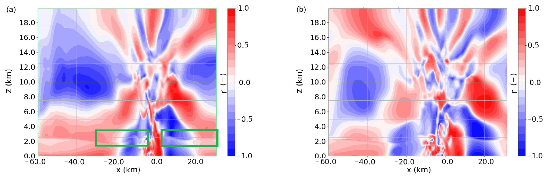
Figure 7Correlation structure between wloc and uavg obtained from the ensemble sensitivity analysis; (a) t=30 min; (b) t=35 min. One can see a gravity wave crest at zi≈2500 m, propagating from x=4 km to x=9 km. With positive vertical velocity perturbations and inbound/converging u winds upon this crest, enhanced forcing for convective initiation (x=4 km, z=3 km, t=30 min, X in Fig. 4b) is correlated with our target variable.
The time evolution of correlation patterns in the squall-line-relative flow up to 25 min (during which statistically significant patterns are not identified) is presented in the Supplement.
After 30 min, small undulations around the initial interface height zi are visible in the correlation patterns, and a crest develops in the immediate wake of the cold pool edge ( km), while ahead of this edge a first signal of gravity waves occurs (x=5 to x=15 km; Fig. 7). Through w, the latter wave signal is associated with the strong convective initiation in ENS-03, which does not occur in the reference simulation. In the next 15 min, additional (faster) gravity wave signals propagate away from the source region. This source region of warm air upstream of the squall line would definitely pass the statistical significance test for t=30 until t=60 min. As the circulation is almost 2D, this is partly inherited by the fact that the circulation in the x–z plane contains both of the lagged variables from the statistical analysis: w at t=30 min and u.
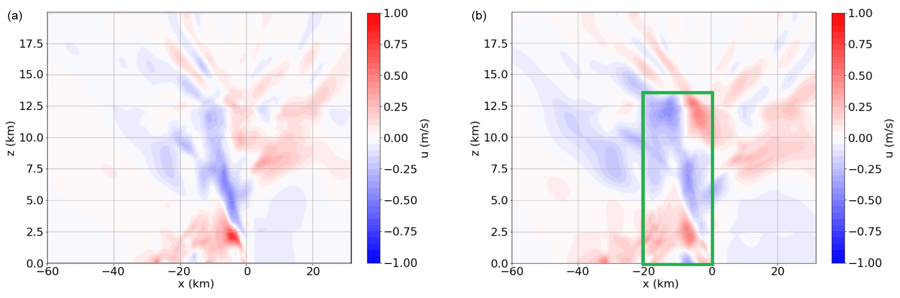
Figure 8Domain with corresponding y-averaged u covariance (relative to the cold pool edge) associated with wloc after (a) t=50 min and (b) t=55 min. Among the main features are enhanced convergence in u around z=2.5 km and km, as well as enhanced divergence from z=7 to z=13 km. On the right, one can see extended divergence patterns (slightly) above z=13 km, which is likely associated with an overshooting cloud top with divergent outflow in u. The central area of squall line circulation (see text) used for significance testing of the identified squall line circulation anomaly is marked with a green rectangle (only right figure).
To investigate the second stage, the focus is shifted from the correlations of the ensemble sensitivity analysis to the second covariant: the along-line average of relative u (depicted in Fig. 8). The signals in u move from upright multi-wavenumber in the vertical, centred at the convective cells, to ones that are aligned with the tilted cold pool and another contribution that causes upper tropospheric divergence away from the cells (in the anvil). Both of these signals of variability associated with the squall line circulation occur after 40–50 min. Synchronously, the associated u variability also exceeds 1 m s−1, maximising at altitudes of 1.5 to 8 km (Fig. 8a). The features of zonal flow still amplify in the higher regions of the troposphere and up to overshooting tops (Fig. 8b), but they also gradually propagate away from their initial location in the following 30–40 min.
After 55 min, the flow perturbation is statistically significant: in the central 20 km of the squall line and at altitudes up to the tropopause a fractional area f of 0.56 passes the statistical significance test at p=0.05 and f=0.35 at p=0.0125 (Fig. 8b). This is more than an order of magnitude larger than random values (see also Wilks, 2016).
After 80 min, the u variability associated with wloc has weakened. Later some renewed variability occurs at t=90 min (see the Supplement).
The circulation revealed by the ensemble sensitivity analysis demonstrates anomalous convergence of mass at z=2–3 km, rearward of the cold pool edge (Fig. 8). The convergence results from enhanced easterly flow in the updraught region which gradually rises and moves upstream relative to the cold pool, due to the updraught tilt. Easterly flow anomalies move upward, extending initially (t=45 min) from the surface to 8–9 km altitude. On its rearward side, a westerly flow anomaly does roughly the same but sticks to lower levels and dissipates earlier.
At the same time, another feature in the sensitivity signal occurs in the upper troposphere: an enhanced upper tropospheric divergence at t=50 min, overshooting into the lowermost stratosphere at t=55 min (Fig. 8). This divergence pattern itself diverges with time and fades outward after about t=80 min (see also the Supplement).
3.3.3 Downdraught variability and cloud tops
In this section the downdraught characteristics are discussed. Furthermore, the cloud-top height is evaluated, and the statistical relations between the diagnostics and the two precursors (wloc and system acceleration to vcp) are quantified.
Downdraught detection
To compute the downdraught mass flux, area and conditional vertical velocities of downdraughts, all grid cells with negative vertical velocities (w<0 m s−1) and a minimal cloud hydrometeor density of kg m−3 were selected. The downdraught area is given by the number of grid cells occupied in each layer. This computation method is adapted from Varble et al. (2020). Subsequently, gravity wave contributions from saturated parcels to downward motion are removed, by removing any grid cells where the total density (ρmoist_air+ρwater) was lower than its horizontal average over that model layer. Downdraught parcels with negative vertical velocity but positive buoyancy would be manifestations of downward-moving parcels with hydrometeor content that would not maintain their negative velocity, given their tendency to accelerate upward. Without the correction for gravity waves, downdraughts are overestimated in the near-tropopause region, where gravity wave activity is leading to substantial vertical transport of air with cloud hydrometeor content that is compensated by nearby reverse motion (see also Pandya and Durran, 1996).
Any grid cell classified as downdraught is then used to calculate conditional mean of the vertical velocity w.
Cloud-top detection
Clouds have been defined by the simulated area fraction of reflectivity over 15 dBz. The relative area covered by the cloud mask just after the convective overshoot (55–60 min, Fig. 5) has been aggregated in time (60–90 min) and along the squall line as a function of z, as the anvil spreads out almost horizontally around equilibrium level. A fractional threshold of 0.1 represents ensemble spread of cloud tops.
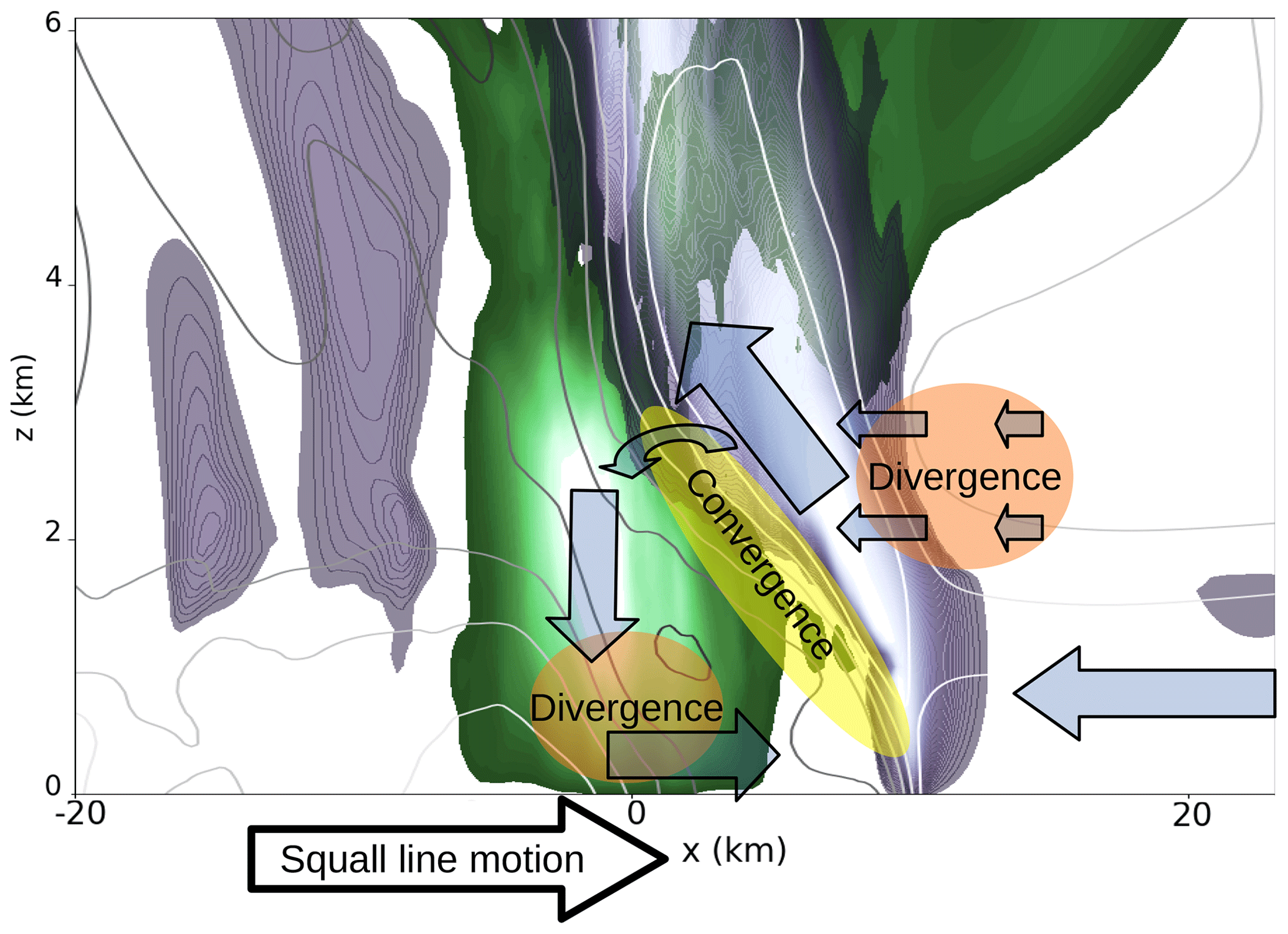
Figure 9Schematic picture of the cold pool circulation in an x–z cross section: green colouring shows updraught mass fluxes, purple colouring shows downdraught mass fluxes. The white isolines indicate easterly flow (−9 m s−1, every 3 m s−1), while darkest grey ones indicate westerly flow (+6 m s−1). One can identify convergence and divergence zones from these contours, which are conceptualised with yellow and orange ovals. The cold-pool-relative flow is given by light blue transparent arrows. Note that the classical pattern of a rear inflow jet (Houze, 2004, and references therein) is practically absent here and that the upper (roughly) half of the troposphere is omitted. The squall line propagation is given by the arrow at the bottom.
Analysis
First, the y-averaged downdraught and updraught fluxes are displayed in Fig. 9 in an x–z cross section for one random ensemble member. This view analytically represents updraught and downdraught fluxes for that simulation and includes a schematic overview of the circulation at low levels. It shows the updraught region on the forward flank of the squall line and a region of horizontal divergence (acceleration) at about 2 km ahead of the main ascent region. A substantial fraction of air masses in the upward branch continue their ascent into the upper troposphere. However, a fraction is entrained in the downdraught region at or behind the cold pool edge. This edge is characterised by a convergence zone between the ascending and descending air. The downdraught, which is located mostly on top of the cold pool, causes low-level divergence and propagation of the squall line and cold pool edge towards the right.

Figure 10Instantaneous profile of squall line downdraughts at t=75 min. (a) Downdraught mass flux, (b) mean conditional w and (c) fractional area. The simulations are coloured in the order of their initial zi, with low interfaces in lime and high interfaces in purple (reference and ENS-03: bold).
Most of the downdraught variability within the ensemble is achieved through downdraught area, as depicted in Fig. 10. The figure shows instantaneous values (at 75 min), in contrast to the temporal averaged used diagnostically. The left panel shows the downdraught mass fluxes, whereas the middle panel describes the conditional vertical velocity and the right most panel the area occupied by the downdraughts. While vertical maxima of the time averaged low-level downdraught fluxes vary by up to 40 %, the area of the downdraughts at the level of maximum fluxes explains about two-thirds of the ensemble variability (even though the low-level temporal mean area varies by only half of that 40 %). Additional contributions to the variability originate mostly from the conditional mean of the downdraught velocity.
In Sect. 3.3.2 a tilted convergence feature was identified, of which the intensity is amplified with increased wloc. A part of the enhanced easterly flow in the updraught regions reaches this convergence zone and leaves the updraught on the upstream side for the convergence zone at the (upstream tilted) cold pool edge. Given the convergence with nearly stagnant air that moves approximately at vcp, the downdraught fluxes below melting level are amplified at km (Fig. 10). The low-level circulation described in this section could be thought of as a sub-circulation within the squall line (Fig. 9): a cold pool circulation. Given the convergence anomaly in Fig. 8, positive covariance of the updraught and downdraught variability within the ensemble is found. That covariance may also imply a response of downdraught mass flux to the secondary convective initiation in Sects. 3.1.1 and 3.2.
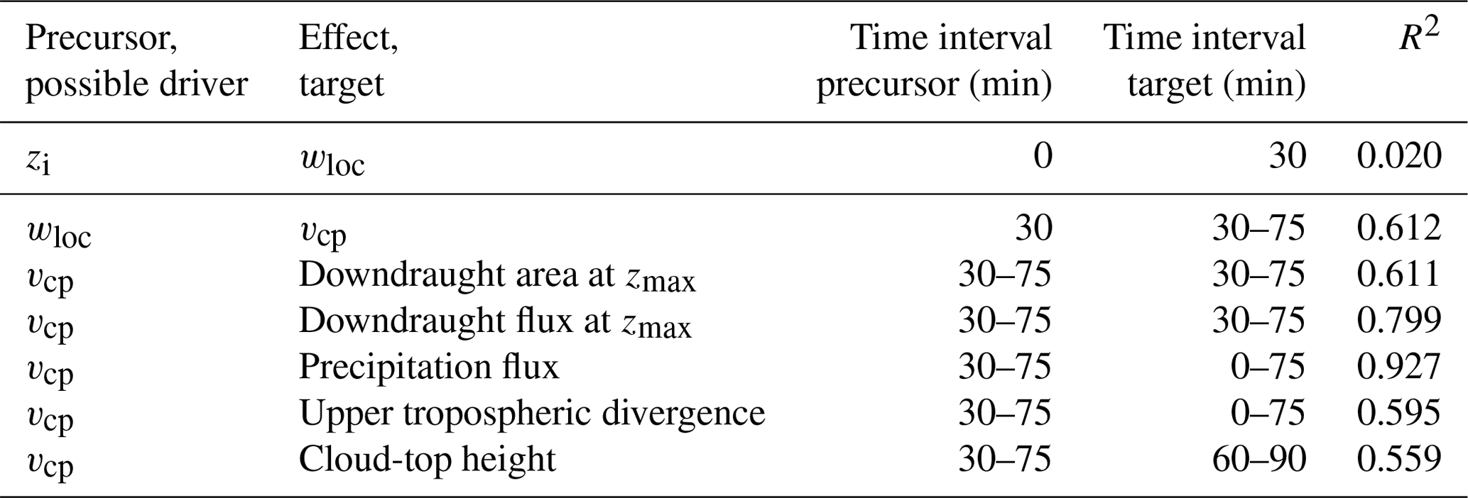
The statistical links between initial perturbations, mean vcp, wloc, downdraught characteristics and other variables are presented in Table 1. Significant correlations between the downdraught properties and wloc are found but not between initial conditions and indicator wloc for the secondary convective initiation. wloc affects convective initiation, relates to overturned mass and in the end to the squall-line-relative flow perturbations. In Sect. 4 these and other connections will be analysed.
Table 1Statistical relations between quantities of interest. R2>0.4 is significant at α=0.05; zi refers to the top height of the shear layer, perturbed in the initial conditions, and Zmax in the table refers to the level where the low-level downdraught flux maximises (z<4 km).
3.4 Error growth in the squall line simulations
In this section the error growth is investigated, i.e. the increasing magnitude of the ensemble spread of the simulated squall lines. The ensemble spread of the horizontal winds with and without a correction for the cold pool propagation is analysed for that purpose. The latter approach allows for a comparison between a quasi-Eulerian and a feature-relative perspective. This enables us to differentiate between a process-based error growth and a feature-location-based increase of the ensemble spread.
A limitation of this method is that only net growth of errors can be detected. Processes can also reduce errors (e.g. diffusion), so the method provides insight only when error growth occurs: a process leading to highly unbalanced tendencies dominates error tendencies: thereby, dominating error growth processes can be identified, and a sequence of error growth processes might be found (Zhang et al., 2007; Baumgart et al., 2019). Negligible initial errors typically lead to error growth to a much wider envelope on long timescales and infinite time limit, which makes the error growth analysis a useful tool here.
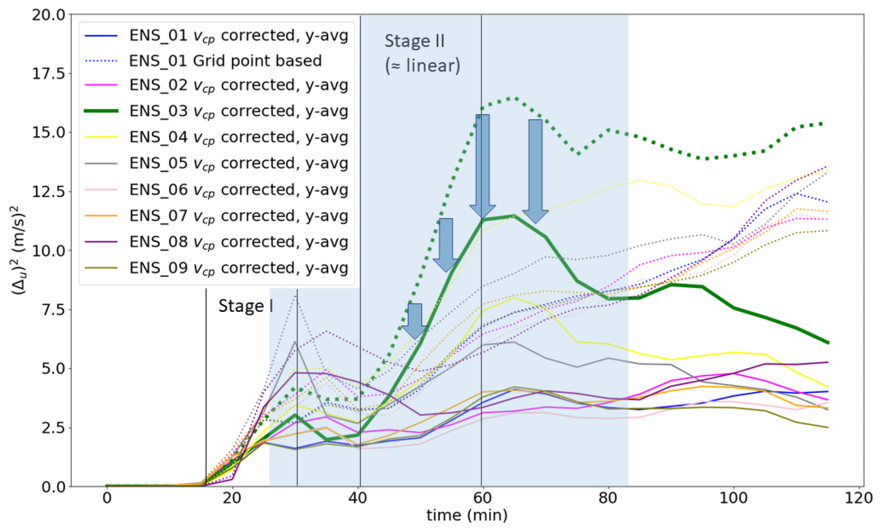
Figure 11Error growth as measured by the ensemble variance in u, where each other member paired with the reference simulation. Both cold pool edge location corrected curves (solid lines) and grid-point-based comparisons (dotted lines) are displayed. Growth stages discussed in the text are also annotated in the figure (see text), and the key interval discussed in the analysis is highlighted by blue shading.
Similar to the ensemble sensitivity, diagnosis of error growth is targeted at variability in squall-line-relative flow and therefore applied to the u winds in the x–z plane. The zonal wind is averaged in the y direction, wherever the cold-pool-relative framework is used. The zonal wind approach differs from a more complete energy metric (Selz, 2019; Zhang et al., 2007; Zhang, 2005), which includes u2 and v2 and may include T. The error growth as a measure of ensemble variability is mapped by the difference in winds between ensemble pairs. The simulations a pair consists of are assumed to fulfil a perfect “error” assumption, analogous to a perfect model assumption (see Selz, 2019): note that only the error needs to fulfil this assumption. Growth rates of error energy are compared here with expected behaviour.
Figure 11 shows the error growth curves. The v component is omitted, as it is comparatively much smaller than u in our scenario; therefore, u reveals the dominant error patterns. Nevertheless, the part of the domain downstream of the squall line is not included. The cold-pool-relative framework allows us to directly compare u winds at x coordinates that are a function of the ensemble member. As the series of x coordinates that can be covered depends on the cold pool position in each ensemble member, about a quarter of the domain is lost by taking the cold-pool-relative view.
A first major stage of growth occurs between t=20 and t=30 min in both the “absolute” and “relative” (Δu)2. This stage of the error growth is likely driven by decorrelation of the gravity wave phase and amplitude and to some extent by differences in the convective initiation (see also Sect. 3.2.2). This early stage causes little variation between the corrected and uncorrected error curves, because the cold pool edge has hardly moved so far. However, variation can occur due to the inclusion of the full domain for the grid-point-based comparison versus only three-quarters of it for the vcp corrected and y-averaged curves.
Another second major stage of error growth occurs from 40 or 45 to 60–65 min. The variability in the squall line flow (Fig. 8) strongly develops during this stage. In this stage the slope between the corrected and uncorrected curves is systematically different, with much larger slopes for the grid-point-based curves. Therefore, a substantial portion of variability in squall-line-relative circulation is probably induced by variability in the cold pool propagation speed (vcp). However, even in the relative framework, some ensemble pairs still demonstrate strong error growth, whereas others hardly show error growth compared to the reference simulation. The impact of non-linearities and feedbacks that affect error growth are present, but during this stage non-linearities do not dominate over vcp effects. Roughly estimated, after about 60 min, a third to half of the error is related to differential cold pool propagation, and another third to half of the total errors was pre-existing at t=30 min. Even though the latter two contributions are not fully independent, this means that non-linearities must be of a magnitude comparable to the two.
Moreover, both the corrected and uncorrected error curves seem to grow linearly in the second stage. In combination with the relatively constant vcp values in each simulation (Sect. 3.3.1), it implies that the cold pool acceleration linearly explains a substantial proportion of variability in the squall line circulation.
Another notable feature between the two identified main stages of error growth in the error growth curves is the relatively low slope of the vcp-corrected curves from 25–30 to 40–45 min. This can be explained by a combination of regions of error growth and other regions where errors decay. Error growth mostly occurs in the regions of secondary convective initiation. The spatial distributions of difference winds strongly suggest that the decay of errors mostly happens at locations of difference wind maxima after 25 min in the upper tropospheric region with cell cores (around x=0 km, not shown). That implies the relatively flat curve after 30–40 min is not inconsistent with local error growth due to secondary convective initiation.
After the first 60–65 min (Fig. 11), the cold pool corrected curves do not grow anymore: errors remain stable. Moreover, the pairs with large (Δu)2 do seem to have a stable vcp-corrected (Δu)2 in the second hour.
Summarising this section, two main stages of error growth have been identified, with no growth in between those two stages of accelerated error growth. The second of two stages reveals interesting near-linear relations with the cold pool edge propagation.
4.1 Evolution of ensemble spread
4.1.1 First amplification of ensemble spread: secondary convective initiation
The ensemble sensitivity analysis has demonstrated statistical correspondence between wloc and flow patterns in the x–z plane elsewhere in time and space. The passive tracers (Sect. 3.2.2) have shown that the updraught position after about 25 min is already associated with differential wloc. The spatio-temporal patterns of a through (respectively crest) in both the tracer distribution and the ensemble sensitivity confirm that the propagation of differences in both amplitude and phase of gravity waves is initiating a vertical velocity difference. This vertical velocity contrast triggers the extension of the convective cells a few kilometres to the east after about 30–35 min – the secondary convective initiation in part of the ensemble and most notably in ENS-03. The secondary initiation impacts convective overturning: subsequently, ENS-03 and the reference simulation reveal a large difference in upward tracer flux of PT2 to levels above 4 km associated with the deep convection.
4.1.2 Second phase in the evolution: cold pool acceleration
After the secondary phase of initiation (30–35 min), the upward mass flux within the convection is not only increased. The cold pool is also accelerated (around 35–45 min) to a speed that is maintained, as suggested by the cold pool edge location and its lag correlation (Sect. 3.3.1). The cold pool velocity is higher for ENS-03 with more convective overturn. It could be anticipated that more convective overturn (updraughts) also leads to increased downdraught intensities. As the strengthening of updraughts is caused by eastward extension of the updraughts, a consequent increase in downdraught area is also expected. Statistics reveal significant intra-ensemble correlation between the maximum downdraught flux as well as downdraught area at the level of maximum downdraught flux (30–75 min) and cold pool velocity (30–75 min).
Further support of the importance of cold pool acceleration in this stage is provided by the error growth curves in Sect. 3.4. The errors start to grow strongly in the gravity wave de-correlation and first convective initiation phase (20 min) and keep growing during the first part of the secondary initiation phase (30–35 min). Directly afterwards, the error growth stagnates shortly (around 35–40 min). Curves where a correction is made for cold pool velocity demonstrate less error growth in the subsequent phase than the uncorrected curves. Feedbacks and interactions other than direct effects of cold pool propagation spread are a source of ensemble variation, but a primary mode of variability within the ensemble is associated with cold pool velocity contrasts. The linear contribution of cold pool propagation is about as important to the errors as other non-linear feedback mechanisms in the second stage of error growth (40–60 min).
The second phase of initiation (30–35 min) and subsequent cold pool acceleration (35–50 min) is the most important event for the ensemble spread.
4.1.3 Common mode of variability and possible common driver
The common driver for a substantial fraction of the squall line variability, including the cold pool acceleration to a stable value of vcp are the gravity waves originating from the first convective initiation. It influences the secondary convective initiation and the cold pool propagation. In the example of strong secondary triggering (ENS-03), convergence originating from the gravity wave crest compensates for upward motion. The convergence below the gravity wave crest implies that the cold air on the rear flank is likely accelerated more eastward relative to the reference member, without secondary initiation. This additional eastward motion leads to more mass reaching the region of initial downdraughts, accelerating the cold pool circulation. This is consistent with Hovmöller diagrams of the cold pool in ENS-03 and the reference simulation, because immediately after the secondary initiation the cold pool in ENS-03 occupies a larger area (the Supplement Fig. S5). Support is also provided by the tracer evolution after 30–35 min. The statistical links between wloc, vcp, and downdraught area and mass flux are confirmed by Table 1 and the convergence patterns in the ensemble analysis.
Overall, this common mode of variability increases the vertical overturning in both upward and downward mass fluxes, by increasing the intensity of the cells. This in turn affects the downdraught strength and leads to precipitation differences. Moreover, the mode of variability probably induces variability in the convective overshooting into the stratosphere after about 60 min and the upper tropospheric divergence (see Table 1; which is consistent with upper tropospheric patterns that could already be found in Fig. 5). Therefore, a common driver of squall line variability exists, of which wloc is an early manifestation.
This wloc is the earliest identified manifestation of the common mode of variability; that is, initial condition differences are uncorrelated with wloc (Table 1), even though it may have been present before this manifestation but hidden in the gravity wave variability. The mode of variability lives on for the next 45–60 min.
4.1.4 Is an intrinsic limit of predictability for the squall line approached?
The tiny initial difference (less than 2 % in terms of shear layer depth) implies that the mode of variability is very sensitive to initial conditions. With a total variability in initial shear layer depth of 5 %, it can be argued in line with Melhauser and Zhang (2012) (based on their Fig. 18) that there can occasionally be an intrinsic limit of predictability on a 1 h timescale. A pattern closely matching such behaviour is exposed by the simulations and analysis, after making a perfect error assumption (see Selz, 2019).
The non-linear behaviour in the evolution from initial conditions to t=30 min show potential presence of an intrinsic limit of predictability. The “random” realisation of gravity wave amplitude and phase after ∼30 min leads to random excitation of the mode of variability: Fig. 4 suggests that amplitude and phase of gravity waves could be directly responsible for differences in wloc. This non-linearity in the evolution between t=0 and t=30 min implies that characteristics of the initial conditions cannot be monotonically linked with the conditions afterwards, including those during the secondary phase of initiation. These resulting conditions include the flow anomalies (or perturbations) associated with the squall line (Fig. 8). Initial perturbations are non-linearly linked with much of the squall line variability after 30–85 min. Therefore, Fig. 18 in Melhauser and Zhang (2012) fits to our findings, and it can be argued that intrinsic sensitivity is a key implication.
4.1.5 Squall line flow perturbations
The flow perturbations in the squall line were very likely affected by wloc and the exposed common mode of variability. It builds up after about 40–45 min of simulation time and its relation with wloc peaked after 55–60 min. The flow anomalies, as shown in Fig. 8, resemble an enhanced circulation of the jump updraught, downdraught and overturning updraught (Moncrieff, 1992). The figure suggests that the mode of variability is partly explained by intensification of this 2D circulation after 45–85 min.
During the second hour of simulations the traces of the identified mode of variability seem to disappear gradually. The gradual dissipation of the initial mode of variability was identified by the ensemble sensitivity analysis between 70 and 85 min, with a new structure of u variability appearing, which is partially opposing the earlier relative flow anomaly. In combination with the flattening error curve in Fig. 11 during the second hour, this might suggest a sign of saturation, where (Δu) reaches about 4 m s−1. That value is a significant fraction of the actual u, but roughly only half of the absolute value. Furthermore, error saturation cannot be addressed properly: the simulation time is too short, as opposed to Weyn and Durran (2017), who properly address error saturation.
The exposed common mode of variability may co-vary with a sub-hourly timescale imposed on the squall line by cyclic behaviour during its growth, as in McAnelly et al. (1997) and Adams-Selin (2020a).
4.2 Discussion
This study identifies a highly relevant window for squall line error growth in the first 80 min of the development, in which systematic variability in the squall-line-relative flow has fully developed and also decays. Nevertheless, the squall lines initiated with a cold pool structure start getting mature only later on in the 120 min simulation. Furthermore, the simulations are restricted to a relatively small domain. Parts of mature and the dissipation state of the system are excluded. Still, this study is able to depict that small errors in the initiation lead to a systematic variability of the convective system. A different set-up (e.g. larger domain, different boundary conditions and an extended simulation time) could provide more insights into the development of ensemble spread during the system's mature phase.
Comparable studies where a discrete propagation event occurs are found in Fovell et al. (2006) and Adams-Selin (2020a, b). The simulation set-up of the latter two studies is closely resembled in our model configuration: our depth of the shear layer is comparatively reduced and the domain and squall line geometry deviates. In our study, new cell grows ahead of the squall line, but a lot earlier than in Adams-Selin (2020a, b), i.e. already after 30 min, just a couple of kilometres ahead of the squall line, as opposed to the clearer separation in Adams-Selin (2020a, b) and Fovell et al. (2006). Quite soon this event resembling discrete propagation is absorbed by the squall line itself. The discrete propagation event detected in Fovell et al. (2006) could not happen as closely ahead of the squall line as here: the model grid spacing was wider then and small updraughts are often at the minimum size possible. However, a distinct convective initiation only about 3 km ahead of a squall line is resolved here. As model grid spacing becomes smaller, discrete propagation can be simulated in LES at 500–1000 m from pre-existing cells, which requires a higher output frequency, as in Adams-Selin (2020a, b).
Even though Weyn and Durran (2017) approach squall line predictability from a different perspective, this study provides an additional foundation on how squall line predictability may be extended very slightly only (on the order of an hour) when initial conditions are very accurately known: initial conditions are non-linearly linked to the secondary phase of convective initiation and the secondary phase of initiation is highly sensitive to these initial conditions. On the other hand, the findings also suggest that some of the information on convective initiation can be stored as linear signals in the squall-line-relative circulation that live for timescales on the order of 1 h. This finding once more confirms the known ideas of shorter and shorter timescales of errors for smaller and smaller scales (Lorenz, 1969; Durran and Gingrich, 2014).
The ensemble in this study starts with highly but not fully 2D initial conditions, as part of a wide spectrum from highly simplified squall line studies (see Houze, 2004, for references) to more recent simulations of real cases coupled to the large scales (e.g. Melhauser and Zhang, 2012). The initial conditions are practically the same as those in Adams-Selin (2020a) apart from the depth of the shear layer. The largely two-dimensional evolution makes the variety of diagnostics applied here much more affordable to assess, which is particularly beneficial in error growth studies. It is not common that squall lines initiate in a time period as short as 10 min along a straight line, as in our idealised setting. Even if not completely representative for many squall lines in the real atmosphere, convergent rolls often organise convection and occur along real squall lines, still concentrating convective initiation. Insights into error growth provided here and in processes responsible for error growth are likely largely applicable along restricted sections of real squall lines, especially those closely relating to findings of Melhauser and Zhang (2012). The idealisation only emphasises signals here, which is of benefit to the analyses.
The robustness of statistical results may appear questionable at the very first glance even after statistical tests, since an ensemble pair is compared in Sect. 3.2 and ensemble size is just n=10. Nonetheless, the very high correlations in Sect. 3.3.2 survive the significance tests with a null hypothesis that correlations are random, verifying the statistical robustness of non-random correlations. Measures with which the ensemble sensitivity analysis survives the tests implied confidence in robust flow anomalies. Statistical test outcomes indicate that a larger ensembles would reveal the same signal as the 10 member ensemble. As confirmed by the uncorrected error growth curves, the exposed mode of variability is well established and well separable from noise and non-linear contributions. These non-linear components consist of the feedbacks that occur to a limited extent. The ensemble sensitivity analysis reveals that the main mode of squall line variability is strongly related to the second phase of convective initiation.
The relations found indicate that cold pool acceleration after about 30 min is very likely explained by the main mode of variability and hence by variability in gravity wave propagation. It could be argued that the depth of heating profile immediately before cold pool acceleration can affect the vertical wavelength and propagation speed of gravity waves of a certain wavenumber, in agreement with findings by Pandya and Durran (1996). A heating profile depth differing by 1 km would provide a variability in cold pool propagation of about 8 %–10 % for a 12 km deep troposphere and explain an 8 %–10 % difference in cold pool propagation speed. If a wave has a vertical wavenumber of over twice the depth of the troposphere or a vertical wavelength of about 10 km, it will propagate at about 17 m s−1. That wavelength is equal to wavenumber one in the layer between the surface cold pool and the tropopause. Against easterly near-surface winds that are on the order of 12–14 m s−1, these gravity waves would propagate eastward relative to this near-surface flow at low speeds of 3–4 m s−1: the density current could surf on this wave. The 1.7 m s−1 difference in propagation velocity between ENS-03 and reference is consistent with this. Inspection of the precursor condensation rates after 25 min (before the gravity wave leads to secondary initiation) suggests a deviation in heating profile depth of at least 500 m between ENS-03 and the reference simulation, probably close to 1 km. Furthermore, cloud-top detections between the two deviate by 800 m after 60–90 min. In other words, there is support for this argument. The arguments are comparable to Grant et al. (2018) and references therein and Stechmann and Majda (2009). Whether the gravity wave propagation leads to differential cold pool acceleration is beyond the scope of our study. A detailed minute-by-minute analysis for the 20–30 min interval (with sub-minute output) is required to address that question, including a computation and analysis of additional quantities such as the Scorer parameter.
This study compares an ensemble of idealised squall line simulations with nearly identical initial conditions. It demonstrates that some degree of linearity in the error growth of the convective event is maintained throughout the second half-hour of the simulation, during which the squall line grows towards the mature stage. A secondary phase of convective initiation after ∼30 min has been identified as crucial for the evolution of the ensemble spread. The mode of variability associated with this second phase of initiation has been identified as shifts in phase and amplitude of gravity waves triggered by the developing squall line itself, originating from the tiny initial disturbances. It is first revealed by the upward motion a few kilometres ahead of the squall line after 30 min. Leading to contrasts in secondary initiation of convection, the effect of this mode of variability on the squall line through upward tracer and mass transport, downward mass transport, cloud-top height, and variability in squall line circulation can be followed. Its effect is most clearly present after 55–60 min of simulation time. After almost an hour of existence, this mode of variability gradually disappears (70–85 min).
In good agreement with Melhauser and Zhang (2012) and Hanley et al. (2013), convective initiation sensitively depends on environmental conditions in our ensemble of idealised simulations. The chain of interactions has been documented in detail: following the crucial secondary initiation phase, a cold pool acceleration is coupled to the intensity of updraughts and downdraughts. On the other hand, once established (35–45 min), the cold pool velocity vcp is maintained throughout the next 30–45 min, as shown by Sect. 3.3.1. Variation in vcp explains much of the subsequent variance in cold pool perpendicular flow (u); therefore, a substantial fraction of it is explained by the mode of variability identified here. Eulerian and feature-centred perspectives show that both the cold pool propagation itself and non-linear feedback mechanisms play a substantial role in the idealised squall line ensemble after 45–60 min.
Consequently, two stages of error growth are identified:
-
de-correlating gravity wave patterns originating from the initial triggering of convection,
-
a stage associated with the main mode of squall line variability, which to a substantial degree depends linearly on vcp and the secondary phase of convective initiation.
Notably, initial condition uncertainties lose their structure, and less than 2 % variation in initial top height of the shear layer zi can result in convective intensities and overturned mass at opposite ends of an ensemble with 5 % initial variation in that zi. Loss of structure (e.g. top row, Table 1) is likely explained by non-linear developments in the gravity waves (phase, amplitude, stage after 20–30 min) as a precursor to the second phase of initiation. This loss of the initial structure can lead to very different squall line developments in the mature stage, and the ensemble can chaotically diverge towards a wider envelope, where information about earlier states is lost. Loss of uncertainty structure within a narrow ensemble of squall line simulations is in good agreement with the picture that Melhauser and Zhang (2012) draw for intrinsic and practical predictability. Compared to their findings, it can be concluded from this study that a tiny sub-space in initial conditions can provide the same ensemble spread as a much wider sub-space: an intrinsic limit of predictability may be present.
The namelist and output dataset of the simulations used for this study are available on request.
The supplement related to this article is available online at: https://doi.org/10.5194/acp-23-565-2023-supplement.
EG designed, conducted and composed the content of this study as part of his PhD project, with contributions from and under the supervision of HT.
At least one of the (co-)authors is a member of the editorial board of Atmospheric Chemistry and Physics. The peer-review process was guided by an independent editor, and the author also has no other competing interests to declare.
Publisher’s note: Copernicus Publications remains neutral with regard to jurisdictional claims in published maps and institutional affiliations.
Parts of this research were conducted using the supercomputer MOGON 2 and advisory services offered by Johannes Gutenberg University Mainz (https://hpc.uni-mainz.de/, last access: 10 January 2023), which is a member of the AHRP (Alliance for High Performance Computing in Rhineland-Palatinate, https://www.ahrp.info/, last access: 10 January 2023) and the Gauss Alliance e.V. The authors gratefully acknowledge the computing time granted on the supercomputer MOGON 2 at Johannes Gutenberg University Mainz (https://hpc.uni-mainz.de/).
The authors would like to thank Michael Riemer, Mirjam Hirt, Annette Miltenberger, Peter Spichtinger, Christopher Polster, Amelie Mayer, Sören Schmidt, and the reviewers for their contributions through constructive feedback and/or suggestions to improve (sections of) the paper, methods, and/or improving the presentation in some figures; we also thank the editor for handling the review process of this paper.
The research leading to these results has been done within the subproject “A1 – Multiscale analysis of the evolution of forecast uncertainty” of the Transregional Collaborative Research Center SFB/TRR 165 “Waves to Weather” funded by the German Research Foundation (DFG). HT acknowledges additional funding from the Carl Zeiss Foundation.
This research has been supported by the Deutsche Forschungsgemeinschaft (Transregional Collaborative Research Center Waves to Weather (grant no. TRR 165)).
This open-access publication was funded by Johannes Gutenberg University Mainz.
This paper was edited by Thijs Heus and reviewed by three anonymous referees.
Adams-Selin, R. D.: Impact of Convectively Generated Low-Frequency Gravity Waves on Evolution of Mesoscale Convective Systems, J. Atmos. Sci., 77, 3441–3460, https://doi.org/10.1175/JAS-D-19-0250.1, 2020a. a, b, c, d, e, f, g, h, i, j, k
Adams-Selin, R. D.: Sensitivity of MCS Low-Frequency Gravity Waves to Microphysical Variations, J. Atmos. Sci., 77, 3461–3477, https://doi.org/10.1175/JAS-D-19-0347.1, 2020b. a, b, c, d, e, f, g, h
Adams-Selin, R. D. and Johnson, R. H.: Examination of Gravity Waves Associated with the 13 March 2003 Bow Echo, Mon. Weather Rev., 141, 3735–3756, https://doi.org/10.1175/MWR-D-12-00343.1, 2013. a
Alfaro, D. A.: Low-Tropospheric Shear in the Structure of Squall Lines: Impacts on Latent Heating under Layer-Lifting Ascent, J. Atmos. Sci., 74, 229–248, https://doi.org/10.1175/JAS-D-16-0168.1, 2017. a
Baumgart, M., Ghinassi, P., Wirth, V., Selz, T., Craig, G. C., and Riemer, M.: Quantitative View on the Processes Governing the Upscale Error Growth up to the Planetary Scale Using a Stochastic Convection Scheme, Mon. Weather Rev., 147, 1713–1731, https://doi.org/10.1175/mwr-d-18-0292.1, 2019. a, b
Bednarczyk, C. N. and Ancell, B. C.: Ensemble Sensitivity Analysis Applied to a Southern Plains Convective Event, Mon. Weather Rev., 143, 230–249, https://doi.org/10.1175/MWR-D-13-00321.1, 2015. a, b, c
Bierdel, L., Selz, T., and Craig, G.: Theoretical aspects of upscale error growth through the mesoscales: an analytical model, Q. J. Roy. Meteorol. Soc., 143, 3048–3059, https://doi.org/10.1002/qj.3160, 2017. a
Bretherton, C. S. and Smolarkiewicz, P. K.: Gravity Waves, Compensating Subsidence and Detrainment around Cumulus Clouds, J. Atmos. Sci., 46, 740–759, https://doi.org/10.1175/1520-0469(1989)046<0740:GWCSAD>2.0.CO;2, 1989. a, b
Bryan, G.: Cloud Model 1. Version 19.8/cm1r19.8, retrieved/downloaded from: https://www2.mmm.ucar.edu/people/bryan/cm1/ (last access: 10 January 2023), 2019. a, b
Bryan, G. H., Wyngaard, J. C., and Fritsch, M. J.: Resolution Requirements for the Simulation of Deep Moist Convection, Mon. Weather Rev/, 131, 2394–2416, 2003. a, b, c
Coniglio, M. C., Stensrud, D. J., and Wicker, L. J.: Effects of upper-level shear on the structure and maintenance of strong quasi-linear mesoscale convective systems, J. Atmos. Sci., 63, 1231–1252, https://doi.org/10.1175/jas3681.1, 2006. a, b, c
Deardorff, J. W.: Stratocumulus-capped mixed layers derived from a three-dimensional model, Bound.-Lay. Meteorol., 18, 495–527, https://doi.org/10.1007/bf00119502, 1980. a
Durran, D. R. and Gingrich, M.: Atmospheric Predictability: Why Butterflies Are Not of Practical Importance, J. Atmos. Sci., 71, 2476–2488, https://doi.org/10.1175/JAS-D-14-0007.1, 2014. a
Fovell, R. G., Mullendore, G. L., and Kim, S.-H.: Discrete Propagation in Numerically Simulated Nocturnal Squall Lines, Mon. Weather Rev., 134, 3735–3752, https://doi.org/10.1175/MWR3268.1, 2006. a, b, c, d
Grant, L. D., Lane, T. P., and van den Heever, S. C.: The role of cold pools in tropical oceanic convective systems, J. Atmos. Sci., 75, 2615–2634, https://doi.org/10.1175/jas-d-17-0352.1, 2018. a, b, c, d, e
Groot, E.: Output data and namelist – README file 'Evolution of squall line variability and error growth in an ensemble of LES', Zenodo [dataset], https://doi.org/10.5281/zenodo.6619313, also available at https://tinyurl.com/groot-tost-22 (last access: 10 January 2023), 2022. a, b
Hanley, K. E., Kirshbaum, D. J., Roberts, N. M., and Leoncini, G.: Sensitivities of a Squall Line over Central Europe in a Convective-Scale Ensemble, Mon. Weather Rev., 141, 112–133, https://doi.org/10.1175/MWR-D-12-00013.1, 2013. a, b, c, d, e, f
Houze, R. A.: Mesoscale convective systems, Rev. Geophys., 42, RG4003, https://doi.org/10.1029/2004rg000150, 2004. a, b, c
Houze, R. A.: 100 Years of Research on Mesoscale Convective Systems, Meteor. Mon., 59, 17.1–17.54, https://doi.org/10.1175/AMSMONOGRAPHS-D-18-0001.1, 2018. a
Lane, T. P. and Reeder, M. J.: Convectively Generated Gravity Waves and Their Effect on the Cloud Environment, J. Atmos. Sci., 58, 2427–2440, https://doi.org/10.1175/1520-0469(2001)058<2427:CGGWAT>2.0.CO;2, 2001. a
Lane, T. P. and Zhang, F.: Coupling between gravity waves and tropical convection at Mesoscales, J. Atmos. Sci., https://doi.org/10.1175/2011JAS3577.1, 2011. a
Langhans, W., Schmidli, J., and Schär, C.: Bulk Convergence of Cloud-Resolving Simulations of Moist Convection over Complex Terrain, J. Atmos. Sci., 69, 2207–2228, https://doi.org/10.1175/JAS-D-11-0252.1, 2012. a
Lebo, Z. J. and Morrison, H.: Effects of Horizontal and Vertical Grid Spacing on Mixing in Simulated Squall Lines and Implications for Convective Strength and Structure, Mon. Weather Rev., 143, 4355–4375, https://doi.org/10.1175/MWR-D-15-0154.1, 2015. a, b, c
Lorenz, E. N.: The predictability of a flow which possesses many scales of motion, Tellus, 21, 289–307, https://doi.org/10.3402/tellusa.v21i3.10086, 1969. a, b
Mapes, B. E.: Gregarious Tropical Convection, J. Atmos. Sci., 50, 2026–2037, https://doi.org/10.1175/1520-0469(1993)050<2026:GTC>2.0.CO;2, 1993. a
McAnelly, R. L., Nachamkin, J. E., Cotton, W. R., and Nicholls, M. E.: Upscale Evolution of MCSs: Doppler Radar Analysis and Analytical Investigation, Mon. Weather Rev., 125, 1083–1110, https://doi.org/10.1175/1520-0493(1997)125<1083:UEOMDR>2.0.CO;2, 1997. a
Melhauser, C. and Zhang, F.: Practical and intrinsic predictability of severe and convective weather at the Mesoscales, J. Atmos. Sci., 69, 3350–3371, https://doi.org/10.1175/jas-d-11-0315.1, 2012. a, b, c, d, e, f, g, h, i, j, k, l
Moncrieff, M. W.: Organized Convective Systems: Archetypal Dynamical Models, Mass and Momentum Flux Theory, and Parametrization, Q. J. Roy. Meteorol. Soc., 118, 819–850, https://doi.org/10.1002/qj.49711850703, 1992. a
Morrison, H., Curry, J. A., and Khvorostyanov, V. I.: A New Double-Moment Microphysics Parameterization for Application in Cloud and Climate Models. Part I: Description, J. Atmos. Sci., 62, 1665–1677, https://doi.org/10.1175/JAS3446.1, 2005. a
Morrison, H., Thompson, G., and Tatarskii, V.: Impact of Cloud Microphysics on the Development of Trailing Stratiform Precipitation in a Simulated Squall Line: Comparison of One- and Two-Moment Schemes, Mon. Weather Rev., 137, 991–1007, https://doi.org/10.1175/2008mwr2556.1, 2009. a, b, c
Nicholls, M. E., Pielke, R. A., and Cotton, W. R.: Thermally Forced Gravity Waves in an Atmosphere at Rest, J. Atmos. Sci., 48, 1869–1884, https://doi.org/10.1175/1520-0469(1991)048<1869:TFGWIA>2.0.CO;2, 1991. a, b
Pandya, R. E. and Durran, D. R.: The influence of convectively generated thermal forcing on the mesoscale circulation around squall lines, J. Atmos. Sci., 53, 2924–2951, https://doi.org/10.1175/1520-0469(1996)053<2924:tiocgt>2.0.co;2, 1996. a, b, c
Rodwell, M. J., Magnusson, L., Bauer, P., Bechtold, P., Bonavita, M., Cardinali, C., Diamantakis, M., Earnshaw, P., Garcia-Mendez, A., Isaksen, L., Källén, E., Klocke, D., Lopez, P., McNally, T., Persson, A., Prates, F., and Wedi, N.: Characteristics of Occasional Poor Medium-Range Weather Forecasts for Europe, B. Am. Meteorol. Soc., 94, 1393–1405, https://doi.org/10.1175/bams-d-12-00099.1, 2013. a
Rotunno, R., Klemp, J. B., and Weisman, M. L.: A theory for strong, long-lived squall lines, J. Atmos. Sci., 45, 463–485, https://doi.org/10.1175/1520-0469(1988)045<0463:atfsll>2.0.co;2, 1988. a, b
Selz, T.: Estimating the Intrinsic Limit of Predictability Using a Stochastic Convection Scheme, J. Atmos. Sci., 76, 757–765, https://doi.org/10.1175/jas-d-17-0373.1, 2019. a, b, c, d, e
Selz, T., Riemer, M., and Craig, G.: The transition from practical to intrinsic predictability of midlatitude weather, J. Atmos. Sci., 79, 2013–2030, https://doi.org/10.1175/JAS-D-21-0271.1, 2022. a, b
Skamarock, W. C.: Evaluating mesoscale NWP models using kinetic energy spectra, Mon. Weather Rev., 132, 3019–3032, https://doi.org/10.1175/mwr2830.1, 2004. a
Stechmann, S. N. and Majda, A. J.: Gravity waves in shear and implications for organized convection, J. Atmos. Sci., 66, 2579–2599, https://doi.org/10.1175/2009JAS2976.1, 2009. a, b
Torn, R. D. and Romine, G. S.: Sensitivity of Central Oklahoma Convection Forecasts to Upstream Potential Vorticity Anomalies during Two Strongly Forced Cases during MPEX, Mon. Weather Rev., 143, 4064–4087, https://doi.org/10.1175/MWR-D-15-0085.1, 2015. a
Varble, A., Zipser, E. J., Fridlind, A. M., Zhu, P., Ackerman, A. S., Chaboureau, J.-P., Collis, S., Fan, J., Hill, A., and Shipway, B.: Evaluation of cloud-resolving and limited area model intercomparison simulations using TWP-ICE observations: 1. Deep convective updraft properties, J. Geophys. Res.-Atmos., 119, 13891–13918, https://doi.org/10.1002/2013JD021371, 2014. a, b
Varble, A., Morrison, H., and Zipser, E.: Effects of Under-Resolved Convective Dynamics on the Evolution of a Squall Line, Mon. Weather Rev., 148, 289–311, https://doi.org/10.1175/MWR-D-19-0187.1, 2020. a, b, c, d, e
Weisman, M. L. and Klemp, J. B.: The Dependence of Numerically Simulated Convective Storms on Vertical Wind Shear and Buoyancy, Mon. Weather Rev., 110, 504–520, https://doi.org/10.1175/1520-0493(1982)110<0504:tdonsc>2.0.co;2, 1982. a, b, c
Weisman, M. L. and Rotunno, R.: “A theory for strong long-lived squall lines” revisited, J. Atmos. Sci., 61, 361–382, https://doi.org/10.1175/1520-0469(2004)061<0361:atfsls>2.0.co;2, 2004. a
Weisman, M. L., Skamarock, W. C., and Klemp, J. B.: The resolution dependence of explicitly modeled convective systems, Mon. Weather Rev., 125, 527–548, https://doi.org/10.1175/1520-0493(1997)125<0527:trdoem>2.0.co;2, 1997. a, b
Weyn, J. A. and Durran, D. R.: The Dependence of the Predictability of Mesoscale Convective Systems on the Horizontal Scale and Amplitude of Initial Errors in Idealized Simulations, J. Atmos. Sci., 74, 2191–2210, https://doi.org/10.1175/JAS-D-17-0006.1, 2017. a, b, c, d, e
Wilks, D. S.: “The Stippling Shows Statistically Significant Grid Points”: How Research Results are Routinely Overstated and Overinterpreted, and What to Do about It, B. Am. Meteorol. Soc., 97, 2263–2273, https://doi.org/10.1175/bams-d-15-00267.1, 2016. a, b
Zhang, F.: Dynamics and structure of mesoscale error covariance of a winter cyclone estimated through short-range ensemble forecasts, Mon. Weather Rev., https://doi.org/10.1175/MWR3009.1, 2005. a, b
Zhang, F., Bei, N., Rotunno, R., Snyder, C., and Epifanio, C. C.: Mesoscale Predictability of Moist Baroclinic Waves: Convection-Permitting Experiments and Multistage Error Growth Dynamics, J. Atmos. Sci., 64, 3579–3594, https://doi.org/10.1175/jas4028.1, 2007. a, b, c
Zhang, F., Sun, Y. Q., Magnusson, L., Buizza, R., Lin, S.-J., Chen, J.-H., and Emanuel, K.: What Is the Predictability Limit of Midlatitude Weather?, J. Atmos. Sci., 76, 1077–1091, https://doi.org/10.1175/JAS-D-18-0269.1, 2019. a