the Creative Commons Attribution 4.0 License.
the Creative Commons Attribution 4.0 License.
 | 12 May 2023
Characteristics of interannual variability in space-based XCO2 global observations
Yifan Guan
Gretchen Keppel-Aleks
Scott C. Doney
Christof Petri
Dave Pollard
Debra Wunch
Frank Hase
Hirofumi Ohyama
Isamu Morino
Justus Notholt
Kei Shiomi
Kim Strong
Rigel Kivi
Matthias Buschmann
Nicholas Deutscher
Paul Wennberg
Ralf Sussmann
Voltaire A. Velazco
Atmospheric carbon dioxide (CO2) accounts for the largest radiative forcing among anthropogenic greenhouse gases. There is, therefore, a pressing need to understand the rate at which CO2 accumulates in the atmosphere, including the interannual variations (IAVs) in this rate. IAV in the CO2 growth rate is a small signal relative to the long-term trend and the mean annual cycle of atmospheric CO2, and IAV is tied to climatic variations that may provide insights into long-term carbon–climate feedbacks. Observations from the Orbiting Carbon Observatory-2 (OCO-2) mission offer a new opportunity to refine our understanding of atmospheric CO2 IAV since the satellite can measure over remote terrestrial regions and the open ocean, where traditional in situ CO2 monitoring is difficult, providing better spatial coverage compared to ground-based monitoring techniques. In this study, we analyze the IAV of column-averaged dry-air CO2 mole fraction (XCO2) from OCO-2 between September 2014 and June 2021. The amplitude of the IAV, which is calculated as the standard deviation of the time series, is up to 1.2 ppm over the continents and around 0.4 ppm over the open ocean. Across all latitudes, the OCO-2-detected XCO2 IAV shows a clear relationship with El Niño–Southern Oscillation (ENSO)-driven variations that originate in the tropics and are transported poleward. Similar, but smoother, zonal patterns of OCO-2 XCO2 IAV time series compared to ground-based in situ observations and with column observations from the Total Carbon Column Observing Network (TCCON) and the Greenhouse Gases Observing Satellite (GOSAT) show that OCO-2 observations can be used reliably to estimate IAV. Furthermore, the extensive spatial coverage of the OCO-2 satellite data leads to smoother IAV time series than those from other datasets, suggesting that OCO-2 provides new capabilities for revealing small IAV signals despite sources of noise and error that are inherent to remote-sensing datasets.
- Article
(5583 KB) - Full-text XML
-
Supplement
(6223 KB) - BibTeX
- EndNote


Increasing atmospheric CO2 concentration from anthropogenic emissions is the major driver of the observed warming of Earth's climate since the industrial revolution (IPCC, 2023). Although CO2 accumulation in the atmosphere generally is ∼45 % of anthropogenic emissions on a multiyear average (Ciais et al., 2013; Friedlingstein et al., 2019), the growth rate shows substantial interannual variability (Conway et al., 1994). The difference between emissions and the atmospheric CO2 growth rate results from net CO2 uptake by oceans and terrestrial ecosystems (Prentice et al., 2001; Doney et al., 2009), and the fluctuations reflect variations in the strength of those sinks due to climate variations (Peters et al., 2017; Friedlingstein et al., 2019). Much research has suggested that interannual variability (IAV) in the growth rate is predominantly due to variations in terrestrial ecosystem carbon uptake (Marcolla et al., 2017), even though the average uptake is roughly comparable between land and ocean (Le Quéré et al., 2009). Existing atmospheric CO2 observations from surface flask sampling and in situ networks have been used to estimate global- and regional-scale interannual variability in CO2 fluxes (Gurney et al., 2008; Peylin et al., 2013; Keppel-Aleks et al., 2014; Piao et al., 2020). We note, however, that the surface-observing network is located primarily at land and coastal sites, and more subtle ocean-flux signals may be obscured by the large IAV in terrestrial fluxes.
Previous analyses of surface CO2 IAV have shown a strong relationship with the phase and intensity of El Niño–Southern Oscillation (ENSO) (Le Quéré et al., 2009; Schwalm et al., 2011). ENSO variations originate from coupled ocean–atmosphere dynamics that are reflected in large wind and sea surface temperature anomalies over the central and eastern Pacific Ocean. ENSO affects the climate of much of the tropics and subtropics via atmospheric teleconnections on timescales of 2–7 years (Timmermann et al., 2018). On land, suppressed precipitation and high temperature associated with positive phases of ENSO (El Niño conditions) suppress CO2 uptake by tropical ecosystems while promoting fires that further reduce the CO2 uptake by land (Feely et al., 2002; McKinley et al., 2004; Piao et al., 2009; Wang et al., 2014). Although of smaller magnitude, the equatorial Pacific Ocean experiences weakening of the easterly trade winds and suppression of ventilation of deep, cold, carbon-rich waters to the surface during an El Niño, reducing the efflux of natural CO2 to the atmosphere (Patra et al., 2005; Chatterjee et al., 2017).
Chatterjee et al. (2017) were able to directly observe the ocean-flux-driven signal on atmospheric CO2 from El Niño for the first time using XCO2 (column-averaged dry-air CO2 mole fraction) observed over the ocean by NASA's OCO-2 satellite. Space-based observations from OCO-2, which was launched in July 2014, provide novel opportunities to characterize the patterns of IAV in XCO2 in areas that were previously not directly observed by existing monitoring networks. The IAV in XCO2 is being used implicitly for flux attribution in inverse modeling studies (Nassar et al., 2011). These exciting results, however, must be tempered by an awareness that atmospheric CO2 IAV is a relatively small signal. For example, IAV in the surface network is about 1 ppm in scale compared to a seasonal amplitude of around 10 ppm at northern high latitudes. OCO-2 measures column-averaged CO2, so its measurements are sensitive to variations in the boundary-layer mole fraction, which is in direct contact with the land or atmospheric fluxes but also variations in the free troposphere and stratosphere, where flux signals are generally smaller than those observed at the surface (Olsen and Randerson, 2004). Furthermore, variations in the free troposphere are expected to have relatively long correlation length scales due to efficient mixing, making it important to consider the spatial scales at which XCO2 observations provide unique information. This is especially important in light of analysis which suggests that the error variance budget in OCO-2 observations is large and contains a substantial spatially coherent signal (Baker et al., 2022; Torres et al., 2019; Mitchell et al., 2023).
In this paper, we analyze XCO2 from OCO-2 to characterize spatiotemporal patterns in IAV at a near-global scale, over both land and ocean, and relate XCO2 variations to ENSO conditions. We contextualize the information contained in OCO-2 observations by comparing them with space-based GOSAT and ground-based Total Carbon Column Observing Network (TCCON) XCO2 and with surface measurements of CO2. Finally, we use these comparisons to emphasize the spatial scales at which the IAV signal emerges from instrumental noise.
2.1 Datasets
2.1.1 OCO-2 observatory
We analyzed IAV in dry-air column-averaged mole-fraction XCO2 inferred from OCO-2 satellite observations. The OCO-2 observatory was launched in July 2014 and has measured passive, reflected solar near-infrared CO2 and O2 absorption spectra using grating spectrometers since September 2014 (Eldering et al., 2017). XCO2 data are retrieved from the measured spectra using the Atmospheric CO2 Observations from Space (ACOS) optimal-estimation algorithm, which is a full-physics algorithm that takes into account XCO2 and other physical parameters, including surface pressure, surface albedo, temperature, and water vapor profile in its state vector (O'Dell et al., 2018). The satellite flies in a polar and sun-synchronous orbit that repeats every 16 d with three different observing modes of OCO-2, namely, nadir (land only, views the ground directly below the spacecraft), glint (over ocean and land, views just off the peak of the specularly reflected sunlight), and target (typically for comparison with specific ground-based or airborne measurements) (Crisp et al., 2012, 2017). We use the version 10 OCO-2 level-2 bias-corrected XCO2 data product from the Goddard Earth Sciences Data and Information Services Center (GES DISC) archive (https://disc.gsfc.nasa.gov/datasets/OCO2_L2_Lite_FP_10r/summary, last access: 1 March 2022), which has been validated with collocated ground-based measurements from TCCON, discussed in more detail in Sect. 2.2. After filtering and bias correction, the OCO-2 XCO2 retrievals agree well with TCCON in the nadir, glint, and target observation modes and generally have absolute median differences of less than 0.4 ppm and root-mean-square differences of less than 1.5 ppm (O'Dell et al., 2018; Wunch et al., 2017).
2.1.2 TCCON
We corroborate patterns of XCO2 IAV from OCO-2 with those from TCCON, a ground-based network of Fourier-transform spectrometers (FTSs) that measure direct solar-absorption spectra in the near infrared (Wunch et al., 2011). Retrievals of XCO2 and other gases are computed using the GGG2014 version of the TCCON standard retrieval algorithm (Wunch et al., 2015), a nonlinear least-squares spectral-fitting algorithm. The TCCON retrievals are tied to the World Meteorological Organization (WMO) X2007 CO2 scale via calibration with aircraft and AirCore profiles above the TCCON sites (Karion et al., 2010; Wunch et al., 2010). This ensures an accuracy and precision of ∼0.6 ppm (1-sigma) throughout the network (Washenfelder et al., 2006; Messerschmidt et al., 2010; Deutscher et al., 2010; Wunch et al., 2010). TCCON has been used widely as a validation standard by providing independent measurements to compare with multiple satellite XCO2 retrievals, including OCO-2. In previous work, Sussmann and Rettinger (2020) demonstrated a concept to retrieve annual growth rates of XCO2 from TCCON data, which are regionally to hemispherically representative in spite of the nonuniform sampling in time and space inherent to the ground-based network. In our study, we focus on IAV in the XCO2 time series from 26 TCCON sites (Table 1 and Fig. 1) that have at least 3 years of observational coverage within the period from September 2014 to June 2021. These TCCON data have been filtered using the standard filter that is based on a measure of cloudiness and that limits the solar-zenith angle. Data are publicly available from the TCCON GGG2014 data archive (https://tccondata.org/, last access: 2 December 2020) hosted by the California Institute of Technology.
Table 1TCCON column-averaged dry-air mole fractions of CO2 (GGG2014 data).

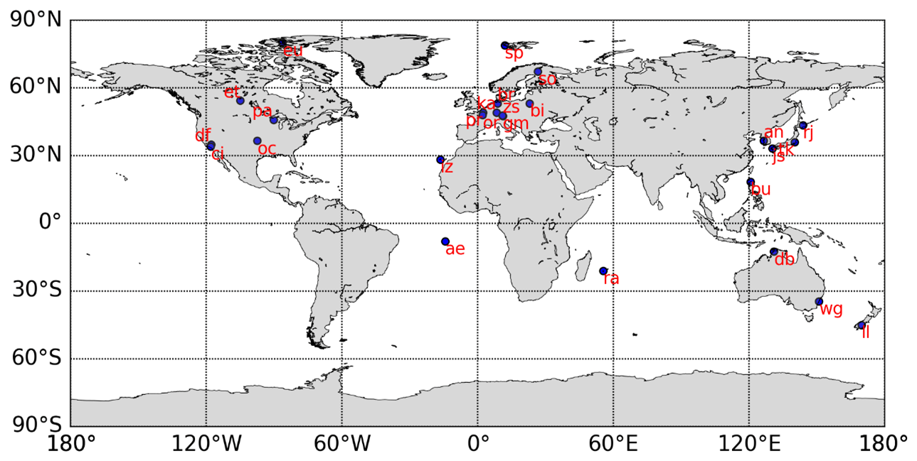
Figure 1Map showing the locations and the abbreviations of the TCCON sites.
2.1.3 Marine-boundary-layer observations
To explore differences in surface and column-averaged CO2 IAV, we analyze IAV in the surface CO2 mole fraction at marine-boundary-layer (MBL) sites in the NOAA (National Oceanic and Atmospheric Administration) cooperative sampling network (https://gml.noaa.gov/dv/site/?program=ccgg, last access: 6 May 2023). At these sites, boundary-layer CO2 is measured using weekly flask samples (Masarie and Tans, 1995; Dlugokencky et al., 2021). MBL sites are typically far away from anthropogenic sources and regions of active terrestrial exchange, so they provide an estimate for large-scale patterns in the global background CO2 concentration. The surface MBL dry-air mole-fraction data have an accuracy level of about 0.1 ppm. In this study, we select 16 sites with at least 80 % data coverage for the approximately 7-year period overlapping with OCO-2 (Table 2 and Fig. 2), and the data are aggregated into four north–south zones for comparison with OCO-2 XCO2: Northern Hemisphere and Southern Hemisphere tropical zones (0–20∘) and Northern Hemisphere/Southern Hemisphere extratropical zones (20–60∘). Each belt contains at least three MBL sites. Higher latitudes (60–90∘) are not considered in this comparison due to the gaps remaining in the OCO-2 XCO2 record at high latitudes during wintertime and shouldering seasons.
Table 2Marine-boundary-layer stations within the NOAA Earth System Research Laboratory CO2 sampling network.
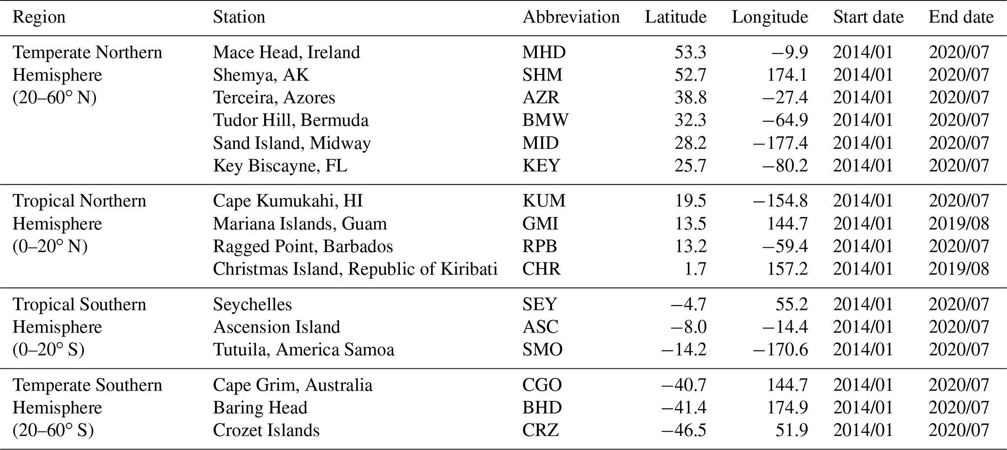
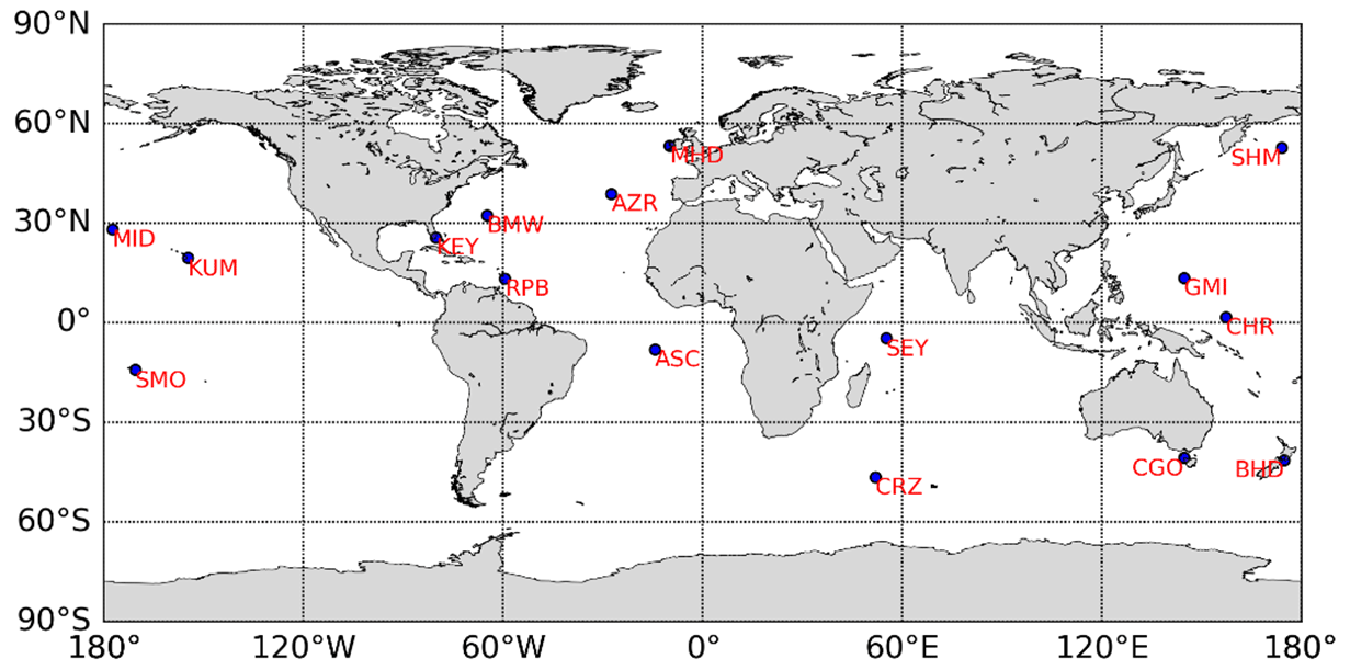
Figure 2Map showing the locations and the abbreviations of the marine-boundary-layer stations within the NOAA Earth System Research Laboratory CO2 sampling network.
2.1.4 GOSAT
We compare patterns of XCO2 IAV from OCO-2 with those from GOSAT. Also known as Ibuki, GOSAT is the world's first satellite dedicated to greenhouse gas monitoring, measuring global total column CO2 and CH4 since 2009 with the Thermal and Near infrared Sensor for carbon Observation (TANSO) FTS on board for greenhouse gas monitoring using three SWIR bands and one TIR band (Cogan et al., 2012; Yoshida et al., 2013). Column-averaged dry mole fractions are obtained at a circular footprint of approximately 10.5 km. GOSAT has a regional bias of approximately 0.3 and 1.7 ppm single observation error versus TCCON (Kulawik et al., 2016). We utilize the FTS SWIR level-3 data global monthly 2.5∘ resolution mean CO2 mixing ratio products from 2009 June to 2021 December to generate IAV and make comparisons with OCO-2. Level-3 products are generated by interpolating, extrapolating, and smoothing the FTS SWIR column-averaged mixing ratios of CO2 and applying the geostatistical calculation technique kriging method. GOSAT observation datasets are available to the public at the NIES GOSAT website (https://www.gosat.nies.go.jp/en/about_5_products.html, last access: 5 August 2022).
2.1.5 Multivariate ENSO index (MEI)
We use the bimonthly MEI (downloaded from the Physical Sciences Laboratory: https://psl.noaa.gov/enso/mei/, last access: 5 April 2023) to explore the relationship between CO2 IAV and ENSO. The MEI is the time series of the leading combined empirical orthogonal function of five different variables (sea level pressure, sea surface temperature, zonal and meridional components of the surface wind, and outgoing longwave radiation) over the tropical Pacific basin. Positive values in the MEI indicate El Niño conditions, while negative values indicate La Niña conditions, and the magnitude reflects the relative strength. Unlike other ENSO indices which use only one climate metric (e.g., the sea level pressure difference between Tahiti and Darwin or the sea surface temperature anomaly within a predefined box), the MEI provides for a more complete and flexible description of the ENSO phenomenon than traditional single-variable ENSO indices and has less vulnerability to errors (Wolter and Timlin, 2011).
2.2 Methods
2.2.1 Spatial aggregation
We aggregate daily XCO2 observations from the version 10 OCO-2 level-2 lite product to the monthly scale, exploring patterns of IAVs at three spatial scales: grid-cell level, zonal averages over 5∘ of latitude, and broad zonal belts. Aggregating soundings reduces random noise in the observations, mitigates the impact of data gaps due to cloud cover, and partly mitigates effects from low winter sunlight levels in polar regions. For grid-cell-level analysis, we aggregate data equatorward of 45∘ to bins since these data are not limited by polar night or degraded by high solar-zenith angles during winter. Poleward of 45∘ in both hemispheres, we aggregate the satellite observation to a latitude–longitude resolution of to compensate for fewer and noisier soundings in these latitudes, especially during winter and its shoulder seasons. Within each or grid cell, only months that have more than five soundings are included in the analysis. Our criteria for aggregation are based on sensitivity experiments in which we modulated the grid-cell resolution from to (Figs. S1 and S2 in the Supplement) and varied the threshold on the required number of soundings within a month from 1 to 25 (Figs. S3–S5 in the Supplement). Our goal was to reduce noise but maintain high spatial coverage (Figs. S6 and S7 in the Supplement). The and aggregations strike the necessary balance of reducing noise (evidenced by the smoother IAV amplitude fields as aggregation increases in Fig. S1) but maintaining spatial information by not oversmoothing (evidenced by the fact that the aggregation occurs at spatial scales finer than the “elbow” where correlations among 1∘ grid cells stop changing with separation distance in Fig. S8 in the Supplement)
In our analysis, we also aggregate data to zonal averages. At intermediate spatial scales, we average all data around the 5∘ latitude bins described above. For comparison with TCCON and MBL data, which are spatially sparse, we further aggregate XCO2 data into four broad zonal belts – each of which contains at least one TCCON or three MBL stations – (delineated in Tables 1 and 2) to assess IAV patterns among the datasets. Keppel-Aleks et al. (2014) showed that drivers of IAV (i.e., temperature, drought stress, or fire) could be attributed when surface CO2 were aggregated into similar broad zonal belts, whereas process-level attribution was not possible with global averaging. We therefore analyze broad zonal belts to gain a large-scale understanding of how three CO2 datasets are similar and where differences lie.
2.2.2 Deriving interannual variations
We use a consistent process to calculate IAV (Eq. 1) from the raw OCO-2, TCCON and MBL time series. The methodology is based on approaches used in Keppel-Aleks et al. (2014) and NOAA curve fitting methodology (Thoning et al., 1989). We decompose the raw time-series data into a long-term trend (which is a function of location (x,y) and time (t)), a seasonal cycle (which is a function of location and calendar month (m)), and IAV anomalies using Eq. (1):
We first fit a third-order polynomial to the raw time series to calculate the observed trend at each location (Fig. 3a). After removing the trend calculated at each grid cell (Fig. 3b), we calculate a mean seasonal cycle by taking the mean value of all January, February, etc., data (Fig. 3c). Particularly at high latitudes, some months are systematically undersampled. For these grid cells, we must have at least 2 years with sufficient observations to calculate a climatological mean for that month; otherwise, that calendar month is assumed to have insufficient data to infer the IAV. Finally, we remove the mean seasonal cycle from the detrended time series at each grid cell to obtain the IAV anomaly time series (Fig. 3d). Given the short data record, we quantify the uncertainty in our calculation of the climatological seasonal cycle as the standard error for each calendar month (blue shading in Fig. 3c), and this uncertainty is propagated to the corresponding IAV time series (Fig. 3d). We fit a third-order polynomial to the raw time series since the GOSAT, MBL, and TCCON time series extend over a decade in length. We confirm that the use of a third-order polynomial versus a second-order polynomial does not remove the IAV signal from the shorter OCO-2 time series (Fig. S9 in the Supplement).
Figure 3Methodology to calculate the CO2 interannual variability time series using OCO-2 XCO2 data at the 5∘ grid cell at 20∘ N, 155∘ W, which contains Moana Loa as an example. (a) 5∘-resolution monthly mean raw OCO-2 XCO2 and the associated third-order polynomial trend. (b) Detrended monthly XCO2 after removing the long-term trend with a repeating 12-month annual cycle obtained from calculating the mean for each month. The light-blue shading gives the uncertainty of the seasonal cycle, which is derived by calculating the standard deviation across all Januaries, Februaries, etc. (c) 12-month mean annual cycle together with the uncertainty range plotted in panel (b). (d) Resulting interannual variability when the mean annual cycle is removed from detrended time series.
3.1 Spatiotemporal variations based on OCO-2 observation
When averaged into broad zonal belts representing the tropics and mid-latitudes, the OCO-2 XCO2 IAV time-series anomalies range between −0.5 and 0.75 ppm (Fig. 4a). All latitude bands show increasing IAV during positive MEI (El Niño) and decreasing IAV during negative MEI (La Niña), although the phasing varies among latitudes. During the strong 2015–2016 El Niño, which began around March 2015 and reached its peak at the start of 2016, XCO2 showed the largest IAV. The Southern Hemisphere extratropical region (Fig. 4d) has a larger and more rapid response in the IAV associated with ENSO compared to other zones, especially for the smaller El Niño that peaked at the beginning of 2020. At this time, the XCO2 IAV time series (Fig. 4d) had an anomaly nearly twice as large as that of other latitude belts (Fig. 4a–c). During both El Niño events, the IAV time series in the Northern Hemisphere tropics zone peaks nearly 6 months after the maximum MEI value.

Figure 4IAV time series averaged for zonal bands between 60∘ N and 60∘ S from four different observing strategies: space-based OCO-2 XCO2 (black), surface CO2 observations from NOAA's marine-boundary-layer (MBL) sites (blue), ground-based TCCON XCO2 (red), and space-based GOSAT XCO2 (grey). (a) Temperate Northern Hemisphere (20–60∘ N), (b) tropical Northern Hemisphere (0–20∘ N), (c) tropical Southern Hemisphere (0–20∘ S), (d) temperate Southern Hemisphere (20–60∘ S). For all panels, the background shading indicates the multivariate ENSO index (MEI), which is positive during El Niño phases.
We assess the spatial correlation patterns with no time lag, 3-month lag, and 6-month lag between the IAV time series and the MEI (Fig. 8a). The XCO2 IAV time series have a strong correlation coefficient with the MEI at both the Southern Hemisphere and Northern Hemisphere low latitudes from 0 to 30∘ N at lag 0, whereas in the Northern Hemisphere extratropics, the maximum positive correlation occurs at month 4 (Fig. 8b). The positive correlation between the MEI and the IAV time series is gradually attenuated, with no clear correlation at 6 months' lag (Fig. 8c).
The differences in temporal phasing between the broad zonal belts (Fig. 4a) associated with El Niño events can be linked to transport of El Niño-driven CO2 flux anomalies away from the tropics when zonal means are calculated from OCO-2 observations at 5∘ latitude resolution (Fig. 5). For the two El Niño periods in 2015–2017 and late 2018 to 2021, high IAV values originate in the tropics, and a smooth transition to high IAV values is seen at higher latitudes as time progresses (Fig. 5a). We note that fluxes outside the tropics may also be influenced by ENSO-related climate variability, yet the transport of tropical-driven anomalies appears to dominate. This 7-year study period also captures the half-year lags for atmospheric transport or climate–ecological teleconnections that impact XCO2 variations in the far north. While the OCO-2 patterns largely conform to the variability expected based on ENSO and are in broad agreement with other observational networks, there are some anomalies that cannot be explained, such as the high XCO2 in early 2020 around 60∘ S (Fig. 5a). Even with more aggressive data filtering, this episode persists, requiring more investigation of unknown geophysical drivers of high XCO2 or potential retrieval issues that could cause a high bias.

Figure 5Hovmöller diagram showing zonal-mean OCO-2 XCO2 IAV time series for 5∘ latitude bins (a) and the zonal standard deviation of XCO2 IAV (b), which gives an estimate of coherence in the IAV patterns among grid cells in the 5∘ zonal belt.
We quantify coherence in CO2 IAV within a latitude circle by taking the standard deviation across grid-cell-level IAV anomalies within each 5∘ latitude zone. The standard deviation among grid cells is highest in the far north, with values as high as 1 ppm poleward of 45∘ N and as low as 0.2 ppm in the southern tropical bands (Fig. 5b), indicating that IAV is less spatially coherent in the Northern Hemisphere. This may be consistent with studies that show greater IAV in terrestrial ecosystem fluxes (concentrated in the Northern Hemisphere) (Zeng et al., 2005) relative to ocean fluxes or may reflect the fact that our IAV time series also retains the imprint of sampling, measurement, and retrieval errors, which become more pronounced at higher latitudes. In general, there is no time-dependent or ENSO-related pattern for the longitudinal variation of IAVs (no obvious changes during the two El Niño periods), which suggests that the variation within each 5∘ band may be approximately stable and does not change substantially with interannual climate events.
The XCO2 IAV amplitude (the standard deviation of the IAV time series) is notably larger over continental grid cells compared to ocean grid cells (Fig. 6). In both hemispheres, the IAV amplitude over subtropical ocean basins is less than 0.4 ppm, while the IAV amplitude over tropical land in Southeast Asia, the Congo forests, and the Amazon basin is about 1 ppm. At higher latitudes, the XCO2 IAV amplitude can exceed 1.2 ppm above deciduous and boreal forests in North America and Eurasia. Higher values over land likely occur due to the active CO2 exchange between the terrestrial ecosystem and the atmosphere, but we cannot rule out that retrievals over land show more variance due to complex topography, albedo, etc., which are elements of the retrieval state vector. Nevertheless, over land areas with low carbon exchange (e.g., Australia, the Middle East, the Sahara), the XCO2 IAV amplitude is nearly at the same low level as the ocean basins. It is worth noting that, for high-latitude regions, including both northern continents and the Southern Ocean, OCO-2 does not obtain observations over a full calendar year (stippled grid cells in Fig. 6) due to polar nights, low light levels, and high solar-zenith angles. The XCO2 IAV amplitudes are less zonally coherent through these regions than those in the tropics and at the mid-latitudes for both land and ocean. When averaging all ocean or land grid cells around a latitude circle, the zonal-mean IAV amplitude over the ocean ranges from 0.3 to 1.0 ppm, while the land IAV amplitude ranges from 0.4 to 1.1 ppm (Fig. 9). Both the land and ocean profiles have similar north–south patterns, with a higher IAV amplitude in the Northern Hemisphere and a lower IAV amplitude in the Southern Hemisphere and small IAV amplitudes in the subtropics of both hemispheres, with more scatter among land grid cells than the ocean (Figs. 5b and 9), suggesting either the influence of local-flux IAV on land or greater error associated with retrievals on land. We note better coherence between the XCO2 IAV time series of each local grid cell and that of zonal-mean XCO2 IAV time series for the ocean, with correlation coefficients of approximately 0.8. In contrast, land grid cells are generally correlated with the zonal mean at around 0.4 to 0.6 (Fig. 10).
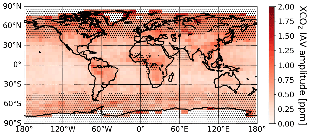
Figure 6OCO-2 XCO2 IAV amplitude, determined as the standard deviation of the IAV time series. Data equatorward of 45∘ are averaged at 5∘ by 5∘ resolution, and data poleward of 45∘ are averaged at 5∘ by 10∘ resolution. Shaded regions indicate grid cells that lack mean annual cycle data for at least 2 calendar months due to polar night or related retrieval challenges.
3.2 OCO-2 XCO2 IAV compared to GOSAT XCO2 IAV
We carried out comparisons between the global spatiotemporal pattern of XCO2 IAV between OCO-2 and GOSAT, since GOSAT has data beginning in 2009. The XCO2 time series from OCO-2 provides higher coverage over midlatitude oceans and tropical rainforests (stippling in Figs. 6 and 7). The IAV amplitude of OCO-2 is generally smaller than that of GOSAT worldwide (Figs. 6 and 7), which may be due to greater data volume and reduced noise in the OCO-2 dataset (Wu et al., 2020). OCO-2 and GOSAT zonal-mean IAV time series generally share the same feature from 2014 to 2021 (Fig. 4a–d), with an increasing trend during El Niño and a decreasing trend during La Niña; however, the GOSAT XCO2 shows a delayed response at the northern midlatitudes, by almost 9 months, to the strong 2015 El Niño compared to the other datasets. Generally, GOSAT IAV time series are nosier, from month to month, compared to those from OCO-2.
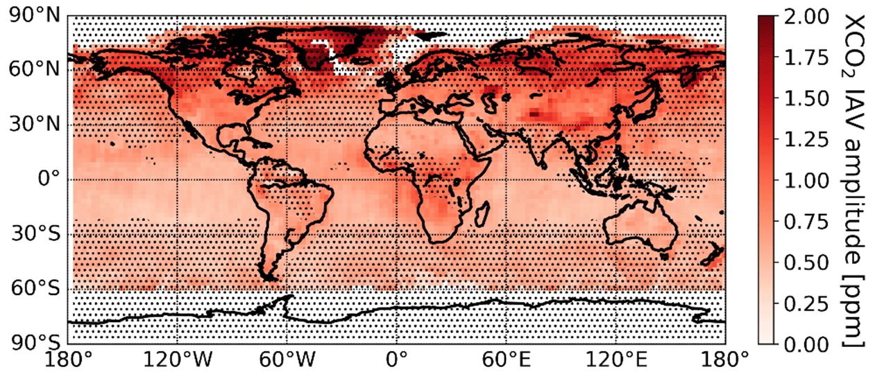
Figure 7Similar to Fig. 6 but based on GOSAT data.

Figure 8Correlation coefficient between local grid-cell OCO-2 XCO2 IAV time series and MEI (a) for synchronous time series, (b) with 3-month lags, and (c) with 6-month lags.
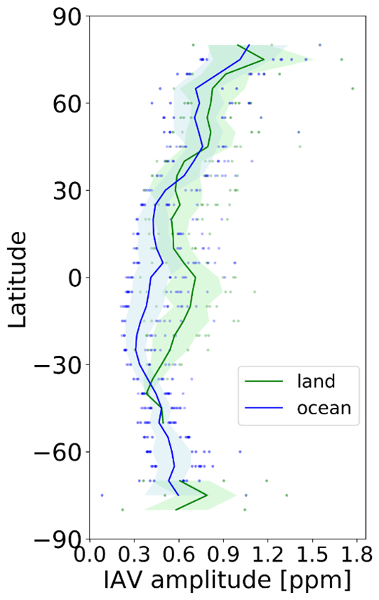
Figure 9Latitudinal profile for the zonal mean of IAV amplitude and the standard deviation among land (green) or ocean (blue) grid cells in each latitude band (shaded area). Individual points represent all grid cells valid in the IAV record within a certain zonal band.
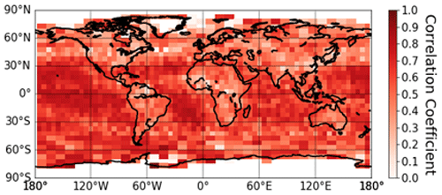
Figure 10Correlation coefficient between local grid-cell IAV time series and the corresponding 5∘ zonal-mean OCO-2 XCO2 IAV time series.
3.3 XCO2 IAV compared to surface and TCCON ground-based sites
Given that the small IAV signal (up to 1 ppm over land and smaller over the ocean) is similar in magnitude to noise and systematic bias in OCO-2 soundings (Torres et al., 2019), we corroborate patterns of IAV from OCO-2 with other datasets. The OCO-2 IAV time series in broad latitudinal belts share similarities with those of TCCON XCO2 and MBL surface CO2 ground-based IAV time series, with all time series showing similar relationships with the MEI. Especially striking is that all time series capture the lagged response in the Northern Hemisphere midlatitude belt to the strong 2015/16 El Niño (Fig. 4a–d). Although the patterns are similar, the magnitude of IAV at the MBL sites is almost double the IAV in the OCO-2 XCO2 time series. Given that the atmospheric boundary layer, where surface observations are made, is on average 10 % of the total column, this suggests that much IAV in total column observations is present within the free troposphere. For TCCON, the amplitude of IAV is similar to that of OCO-2, since both methods capture total column variations. We note that the zonal IAV time series for MBL and TCCON appear to have more high-frequency variations than those from OCO-2 (Figs. S10–S12 in the Supplement), which likely stems from the fact that the zonal composites are developed from sparse ground-based sites (between 1 and 12 observatories) within each latitude belt, whereas the satellite measures at all longitudes within a belt though with more limited time resolution. The zonal-mean OCO-2 observations are correlated with MBL sites within the same latitude band with R between 0.5 and 0.75 (diagonal elements in Fig. 13b). Correlations between zonal TCCON and OCO-2 observations range between 0.15 and 0.55 (Table S1 in the Supplement). The correlations are weakest in the northern tropical band, where TCCON data were unavailable during the strong El Niño (Fig. 3c). It is noteworthy that OCO-2 zonal averages are more correlated among different latitudes than are MBL or TCCON observations (off-diagonal elements in Fig. 13c–e). The greater correlation across latitudes for OCO-2 compared to MBL sites is likely due to the sensitivity of the OCO-2 XCO2 observations to the free troposphere, where meridional transport is more rapid than at the surface. While TCCON data are also sensitive to the free troposphere, we hypothesize that the zonal-belt averages for TCCON, constructed from only a few sites, are more affected by noise, both instrumental and geophysical, and thus show lower coherence than the OCO-2 XCO2 averages constructed from the whole latitudinal bands.
We further compared the IAV from OCO-2 XCO2 with TCCON stations at the site level (Fig. 12). Across all the sites, the IAV amplitude generally shows good agreement and lies between 0.4 and 1.2 ppm. We note a slight low-IAV amplitude in OCO-2 relative to TCCON for all five sites in the Southern Hemisphere which lie below the one-to-one line. Low OCO-2 IAV amplitudes may be due to the fact that a grid cell encompassing these near-coastal locations includes both land and ocean OCO-2 soundings and may be due to specific sources of variance from retrieval bias affected by surface type for OCO-2 (e.g., Fig. 9). It is also worth noting that OCO-2 looks at a region of 5∘ by 5∘ grid cells (or 5∘ by 10∘ at higher latitudes) around TCCON sites, so there are different signals affecting the variance between the two types of observations.
We derive the regression slopes and correlation coefficient R between OCO-2 and monthly averaged TCCON IAV through bootstrapping linear-regression fitting techniques to investigate the coherence between IAV signals from space-based and in situ ground-based observations. We compute the linear regression 1000 times by iteratively resampling the IAV time series with replacement and calculate the 95 % significance level for regression slopes based on the histogram of the sample distributions during the bootstrapping (Fig. S13 in the Supplement). Despite having similar IAV amplitudes, the IAV time series from OCO-2 are only moderately correlated with those from TCCON (Fig. 11). The regression slopes range from 0.1 to 0.6, and R values are generally around 0.1–0.5, indicating that less than 25 % of the IAV in OCO-2 is explained by IAV measured by TCCON. These R values are, as expected, smaller than the zonal averages shown in Fig. 11b, which average some of the site-level noise for TCCON and grid-cell-level noise for OCO-2. The detailed XCO2 IAV time series of each site (Fig. S10) for OCO-2 and TCCON show that the IAV time series in the Northern Hemisphere are more variable, which can partly explain the hemispheric difference in amplitude, slope, and correlation coefficients.
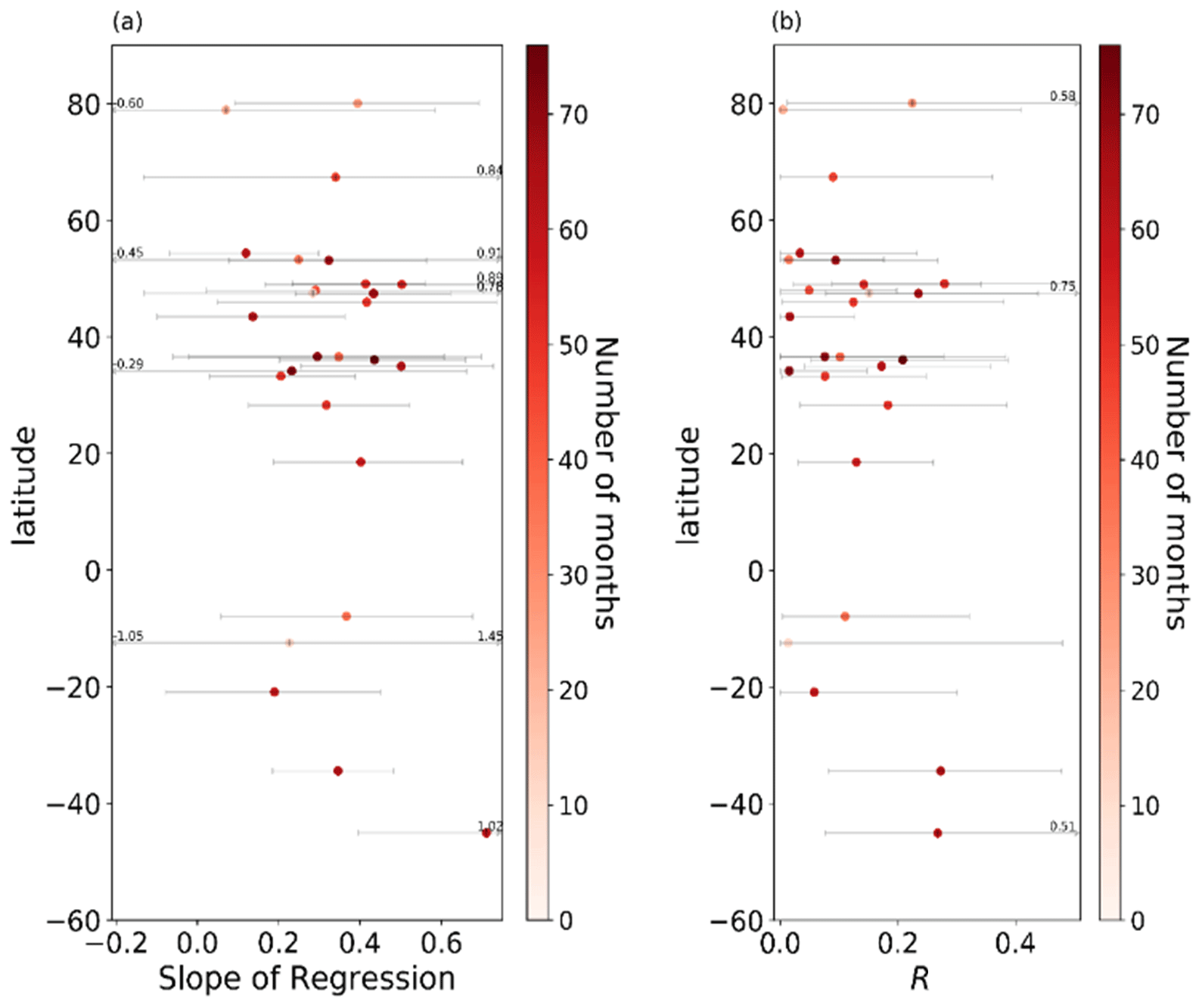
Figure 11Latitudinal profile of regression slope (panel a) and correlation coefficient (R, panel b) of OCO-2 versus TCCON XCO2 IAV. The slope and R values are based on using monthly XCO2 IAV. The error bars result from a Monte Carlo bootstrapping approach. The colors represent the number of months of data which are used for the regression calculation given gaps in both the OCO-2 and TCCON datasets.
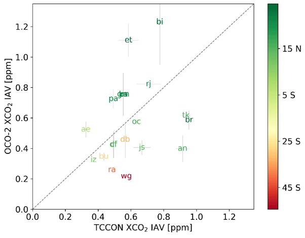
Figure 12Comparison of OCO-2 and TCCON XCO2 IAV amplitude at individual sites. Colors reflect site latitudes. The grey dashed line is the one-to-one identity line. The grey solid line is the error bar of the IAV amplitude.
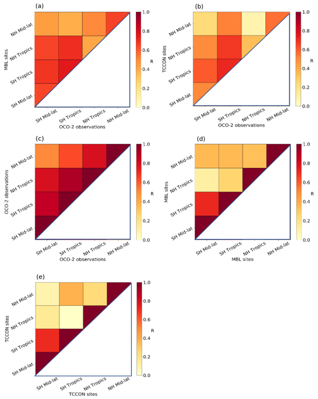
Figure 13Correlation coefficient (R) between mean CO2 time series using three observing strategies. Panel (a) shows the correlation between zonal-mean OCO-2 XCO2 IAV and zonal-mean marine-boundary-layer CO2. Panel (b) shows the correlation between zonal-mean XCO2 IAV from OCO-2 and TCCON. Panels (c–e) show the correlation in zonal-mean IAV time series across four latitude bands for a single observing strategy. Panel (c) shows OCO-2 XCO2, panel (d) shows MBL CO2, and panel (e) shows TCCON XCO2. For panels (c–e), the diagonal elements are 1 by construction. Zonal bands include the tropical (0–20∘) and Northern Hemisphere/Southern Hemisphere temperate (20–60∘) zones.
We use 7 years of OCO-2 total column carbon dioxide observations from late 2014 to mid 2021 to illustrate the global temporal–spatial patterns of atmospheric XCO2 interannual variations. OCO-2 and GOSAT showed reasonable agreement (Fig. 4) in Northern Hemisphere and Southern Hemisphere tropical zones (0–20∘), although there were some notable phase differences during the strong 2015 El Niño for GOSAT compared to the other time series in both the northern and southern extratropical regions. In contrast, OCO-2 shows good temporal agreement with the ground-based observations from the MBL and TCCON. The temporal agreement of the OCO-2 and TCCON XCO2 IAV time series and the MBL surface CO2 IAV time series in broad zonal belts improves our confidence that we can quantify IAV time series from the satellite record. We note that amplitude differences remain among the time series, owing to two major factors: first, compared to MBL surface observations, we expect XCO2 time series to have smaller amplitudes of variability since it integrates over the entire atmospheric column (Olsen and Randerson, 2004), and second, the fact that the OCO-2 time-series averages around a full-latitude circle rather than a few discrete sites reduce some of the IAV contained in site-level records. From the space-based and ground-based detection, we are able to characterize the global response of OCO-2 and TCCON XCO2 or MBL surface CO2 IAV to ENSO and track the CO2 IAV against the positive/negative phase of ENSO, together with the transport of the signal from south to north (Fig. 4). All the datasets show consistent patterns in the response to the El Niño periods, although we note that the IAV amplitude is a factor of almost 2 smaller in the column-averaged mole fraction compared to the boundary-layer CO2, which reflects the fact that IAV variations emerge due to surface fluxes in the lower part of the atmosphere (Olsen and Randerson, 2004) but are efficiently transported into the free troposphere, which comprises the bulk of the column. When taken together, the use of surface and column data may allow better separation of transport-driven versus local flux-driven variations at the interannual timescale. In the future, as partial column retrievals (e.g., Kulawik et al., 2017) mature, intercomparisons of the lowermost tropospheric partial columns may provide a useful bridge between variations in surface MBL observations and total column observations.
Our results, however, underscore the difficulty in detecting IAV signals from remote sensing of XCO2 – while Northern Hemisphere seasonal amplitudes are typically 10 ppm in scale (Basu et al., 2011), the magnitude of OCO-2-detected XCO2 IAV is almost an order of magnitude smaller (less than 0.4 ppm over the ocean and about 1 ppm over continents). The magnitude of IAV is therefore comparable to other components of the XCO2 variance budget; for instance, Torres et al. (2019) show random noise in individual OCO-2 soundings of about 0.3 ppm in the Southern Hemisphere and about 0.7 ppm in the Northern Hemisphere and spatially coherent errors in the retrievals ranging from 0.3 to 0.8 ppm (Torres et al., 2019). Moreover, the uncertainty which originally comes from the varying climatological seasonal cycle can also reach a level of 0.5 ppm (Fig. 3d). Therefore, robust partitioning of IAV from the observed XCO2 signal at a given location requires a comprehensive variance budget (Mitchell et al., 2023), and efforts to infer interannual variations in fluxes from OCO-2 must take grid-cell-level variance into account or leverage zonally averaged data, which are characterized by greater separation between IAV signal and noise.
Our analysis shows that proper spatial averaging of the monthly XCO2 signal can mitigate the imprint of random noise and systematic effects from weather systems at submonthly timescales. Based on sensitivity tests, we recommend averaging low- to mid-latitude XCO2 (equatorward of 45∘) to bins and a grid cell poleward of 45∘, ensuring that each grid-cell aggregates at least five soundings within a month. At these levels of spatial averaging, the XCO2 IAV amplitude was comparable to that of the co-located ground-based XCO2 IAV amplitude measured by TCCON (Fig. 12). However, the moderate to low correlation between the IAV time series from each monitoring platform reveals the discrepancies of the two measurements in sampling, detection, or retrieval, suggesting that one or both is still convolving another source of variance with the calculated IAV signal. Based on the good agreement between the two time series in broad zonal belts, we expect that random noise in both observations may degrade the comparison.
The smaller coherence in the IAV time series in nearby land and ocean grid cells may be due to larger error over land or may reflect the fact that XCO2 observations over land contain information about heterogeneous local-flux IAV. Complete analysis of the variance budget for OCO-2 observations (Mitchell et al., 2023) will elucidate the likely imprint of each process. When using IAV time series for flux inference, it will be crucial to account for non-flux imprints such as imprint from atmospheric transport, random errors, systematic errors, and remote geophysical coherence on the time series (e.g., Torres et al., 2019; Mitchell et al., 2023), since spurious attribution of IAV will lead to biased fluxes.
We examined IAV in OCO-2 data to determine whether the small variations that result from interannual flux variations can be detected in light of other sources of variance in the space-based dataset. Our results show that zonal averages reveal relationships with ENSO that are consistent with those from an established ground-based monitoring network. Zonal averages greatly reduce random noise in XCO2 compared to averages. In general, OCO-2 can successfully monitor CO2 IAV over both land and ocean, contributing important spatial coverage beyond inferences of IAV from existing ground-based networks.
The version 10 OCO-2 level-2 bias-corrected XCO2 data product is available from the Goddard Earth Sciences Data and Information Services Center Archive: https://disc.gsfc.nasa.gov/datasets/OCO2_L2_Lite_FP_10r/summary (GES DISC, 2022). TCCON data are publicly available from the TCCON data archive (https://doi.org/10.14291/TCCON.GGG2014, Total Carbon Column Observing Network (TCCON) Team, 2017) hosted by the California Institute of Technology. MBL dry-air mole-fraction data are available from the NOAA Global Monitoring Laboratory Earth System Research Laboratories Archive: https://doi.org/10.15138/YAF1-BK21 (https://gml.noaa.gov/ccgg/mbl/data.php, last access: 17 February 2023, NOAA GML CCGG Group, 2019). GOSAT observation datasets are available to the public at the NIES GOSAT website (https://www.gosat.nies.go.jp/en/about_5_products.html, JAXA et al., 2022).
The supplement related to this article is available online at: https://doi.org/10.5194/acp-23-5355-2023-supplement.
Formal analysis: YG. Writing – original draft preparation: YG. Conceptualization: GKA. Supervision: GKA. Project administration: GKA and SCD. Writing – review and editing: GKA, SCD, CP, DP, DW, FH, HO, IM, JN, KeS, KiS, KR, MB, ND, PW, RS, VAV, and YT.
The contact author has declared that none of the authors has any competing interests.
Publisher's note: Copernicus Publications remains neutral with regard to jurisdictional claims in published maps and institutional affiliations.
The authors thank the participants of the NASA OCO-2 mission for providing the OCO-2 data product (from the GES DISC archive: https://disc.gsfc.nasa.gov/datasets/OCO2_L2_Lite_FP_10r/summary, last access: 1 March 2022) used in this study. We thank the TCCON partners for providing total column data. The Paris TCCON site has received funding from Sorbonne Université, the French research center CNRS, the French space agency CNES, and Région Île-de-France. TCCON sites at Tsukuba, Rikubetsu, and Burgos are supported in part by the GOSAT series project. Burgos is supported in part by the Energy Development Corp. Philippines, and the TCCON site at Réunion has been operated by the Royal Belgian Institute for Space Aeronomy with financial support since 2014 by the EU project ICOS-Inwire and the ministerial decree for ICOS (FR/35/IC1 to FR/35/C6) and local activities supported by LACy/UMR8105 and by OSU-R/UMS3365 – Université de La Réunion. The TCCON stations at Garmisch and Zugspitze have been supported by the Helmholtz Society via the research program “Changing Earth – Sustaining our Future”. The Eureka TCCON measurements were made at the Polar Environment Atmospheric Research Laboratory (PEARL) by the Canadian Network for the Detection of Atmospheric Change (CANDAC), primarily supported by the Natural Sciences and Engineering Research Council of Canada, Environment and Climate Change Canada, and the Canadian Space Agency.
This research was funded by NASA Awards (grant nos. 80NSSC18K0900 and 80NSSC21K1070) to the University of Michigan and (grant nos. 80NSSC18K0897 and 80NSSC21K1071) to the University of Virginia.
This paper was edited by Ronald Cohen and reviewed by Christopher O'Dell and two anonymous referees.
Baker, D. F., Bell, E., Davis, K. J., Campbell, J. F., Lin, B., and Dobler, J.: A new exponentially decaying error correlation model for assimilating OCO-2 column-average CO2 data using a length scale computed from airborne lidar measurements, Geosci. Model Dev., 15, 649–668, https://doi.org/10.5194/gmd-15-649-2022, 2022.
Basu, S., Houweling, S., Peters, W., Sweeney, C., Machida, T., Maksyutov, S., Patra, P. K., Saito, R., Chevallier, F., Niwa, Y., Matsueda, H., and Sawa, Y.: The seasonal cycle amplitude of total column CO2: Factors behind the model-observation mismatch, J. Geophys. Res.-Atmos., 116, D23306, https://doi.org/10.1029/2011JD016124, 2011.
Blumenstock, T., Hase, F., Schneider, M., García, O. E., and Sepúlveda, E.: TCCON data from Izana (ES), Release GGG2014.R1 (R1), https://doi.org/10.14291/TCCON. GGG2014.IZANA01.R1, 2017.
Chatterjee, A., Gierach, M. M., Sutton, A. J., Feely, R. A., Crisp, D., Eldering, A., Gunson, M. R., O'Dell, C. W., Stephens, B. B., and Schimel, D. S.: Influence of El Niño on atmospheric CO2 over the tropical Pacific Ocean: Findings from NASA's OCO-2 mission, Science, 358, eaam5776, https://doi.org/10.1126/science.aam5776, 2017.
Ciais, P., Sabine, C., Bala, G., and Peters, W.: Carbon and Other Biogeochemical Cycles, in: Climate Change 2013: The Physical Science Basis. Contribution of Working Group I to the Fifth Assessment Report of the Intergovernmental Panel on Climate Change, Cambridge University Press, 465–570, https://doi.org/10.1017/CBO9781107415324.015, 2013.
Cogan, A. J., Boesch, H., Parker, R. J., Feng, L., Palmer, P. I., Blavier, J.-F. L., Deutscher, N. M., Macatangay, R., Notholt, J., Roehl, C., Warneke, T., and Wunch, D.: Atmospheric carbon dioxide retrieved from the Greenhouse gases Observing SATellite (GOSAT): Comparison with ground-based TCCON observations and GEOS-Chem model calculations, J. Geophys. Res.-Atmos., 117, D21301, https://doi.org/10.1029/2012JD018087, 2012.
Conway, T. J., Tans, P. P., Waterman, L. S., Thoning, K. W., Kitzis, D. R., Masarie, K. A., and Zhang, N.: Evidence for interannual variability of the carbon cycle from the National Oceanic and Atmospheric Administration/Climate Monitoring and Diagnostics Laboratory Global Air Sampling Network, J. Geophys. Res.-Atmos., 99, 22831–22855, https://doi.org/10.1029/94JD01951, 1994.
Crisp, D., Fisher, B. M., O'Dell, C., Frankenberg, C., Basilio, R., Bösch, H., Brown, L. R., Castano, R., Connor, B., Deutscher, N. M., Eldering, A., Griffith, D., Gunson, M., Kuze, A., Mandrake, L., McDuffie, J., Messerschmidt, J., Miller, C. E., Morino, I., Natraj, V., Notholt, J., O'Brien, D. M., Oyafuso, F., Polonsky, I., Robinson, J., Salawitch, R., Sherlock, V., Smyth, M., Suto, H., Taylor, T. E., Thompson, D. R., Wennberg, P. O., Wunch, D., and Yung, Y. L.: The ACOS CO2 retrieval algorithm – Part II: Global data characterization, Atmos. Meas. Tech., 5, 687–707, https://doi.org/10.5194/amt-5-687-2012, 2012.
Crisp, D., Pollock, H. R., Rosenberg, R., Chapsky, L., Lee, R. A. M., Oyafuso, F. A., Frankenberg, C., O'Dell, C. W., Bruegge, C. J., Doran, G. B., Eldering, A., Fisher, B. M., Fu, D., Gunson, M. R., Mandrake, L., Osterman, G. B., Schwandner, F. M., Sun, K., Taylor, T. E., Wennberg, P. O., and Wunch, D.: The on-orbit performance of the Orbiting Carbon Observatory-2 (OCO-2) instrument and its radiometrically calibrated products, Atmos. Meas. Tech., 10, 59–81, https://doi.org/10.5194/amt-10-59-2017, 2017.
De Mazière, M., Sha, M. K., Desmet, F., Hermans, C., Scolas, F., Kumps, N., Metzger, J.-M., Duflot, V., and Cammas, J.-P.: TCCON data from Réunion Island (RE), Release GGG2014.R1 (R1), https://doi.org/10.14291/TCCON.GGG2014.REUNION01.R1, 2017.
Deutscher, N. M., Griffith, D. W. T., Bryant, G. W., Wennberg, P. O., Toon, G. C., Washenfelder, R. A., Keppel-Aleks, G., Wunch, D., Yavin, Y., Allen, N. T., Blavier, J.-F., Jiménez, R., Daube, B. C., Bright, A. V., Matross, D. M., Wofsy, S. C., and Park, S.: Total column CO2 measurements at Darwin, Australia – site description and calibration against in situ aircraft profiles, Atmospheric Measurement Techniques, 3, 947–958, https://doi.org/10.5194/amt-3-947-2010, 2010.
Deutscher, N. M., Notholt, J., Messerschmidt, J., Weinzierl, C., Warneke, T., Petri, C., and Grupe, P.: TCCON data from Bialystok (PL), Release GGG2014.R2 (R2), https://doi.org/ 10.14291/TCCON.GGG2014.BIALYSTOK01.R2, 2019.
Dlugokencky, E. J., Crotwell, A. M., Mund, J. W., Crotwell, M. J., and Thoning, K. W.: Atmospheric Nitrous Oxide Dry Air Mole Fractions from the NOAA GML Carbon Cycle Cooperative Global Air Sampling Network, 1997–2020, Version: 2021-07-30, NOAA Global Monitoring Laboratory Data Repository [data set], https://doi.org/10.14291/TCCON. GGG2014.BIALYSTOK01.R2, 2021.
Doney, S. C., Lima, I., Feely, R. A., Glover, D. M., Lindsay, K., Mahowald, N., Moore, J. K., and Wanninkhof, R.: Mechanisms governing interannual variability in upper-ocean inorganic carbon system and air–sea CO2 fluxes: Physical climate and atmospheric dust, Deep-Sea Res. Pt. II, 56, 640–655, https://doi.org/10.1016/j.dsr2.2008.12.006, 2009.
Eldering, A., O'Dell, C. W., Wennberg, P. O., Crisp, D., Gunson, M. R., Viatte, C., Avis, C., Braverman, A., Castano, R., Chang, A., Chapsky, L., Cheng, C., Connor, B., Dang, L., Doran, G., Fisher, B., Frankenberg, C., Fu, D., Granat, R., Hobbs, J., Lee, R. A. M., Mandrake, L., McDuffie, J., Miller, C. E., Myers, V., Natraj, V., O'Brien, D., Osterman, G. B., Oyafuso, F., Payne, V. H., Pollock, H. R., Polonsky, I., Roehl, C. M., Rosenberg, R., Schwandner, F., Smyth, M., Tang, V., Taylor, T. E., To, C., Wunch, D., and Yoshimizu, J.: The Orbiting Carbon Observatory-2: first 18 months of science data products, Atmos. Meas. Tech., 10, 549–563, https://doi.org/10.5194/amt-10-549-2017, 2017.
Feely, R. A., Boutin, J., Cosca, C. E., Dandonneau, Y., Etcheto, J., Inoue, H. Y., Ishii, M., Quéré, C. L., Mackey, D. J., McPhaden, M., Metzl, N., Poisson, A., and Wanninkhof, R.: Seasonal and interannual variability of CO2 in the equatorial Pacific, Deep-Sea Res. Pt. II, 49, 2443–2469, https://doi.org/10.1016/S0967-0645(02)00044-9, 2002.
Feist, D. G., Arnold, S. G., John, N., and Geibel, M. C.: TCCON data from Ascension Island (SH), Release GGG2014.R0 (GGG2014.R0), https://doi.org/10.14291/TCCON.GGG2014. ASCENSION01.R0/1149285, 2014.
Friedlingstein, P., Jones, M. W., O'Sullivan, M., Andrew, R. M., Hauck, J., Peters, G. P., Peters, W., Pongratz, J., Sitch, S., Le Quéré, C., Bakker, D. C. E., Canadell, J. G., Ciais, P., Jackson, R. B., Anthoni, P., Barbero, L., Bastos, A., Bastrikov, V., Becker, M., Bopp, L., Buitenhuis, E., Chandra, N., Chevallier, F., Chini, L. P., Currie, K. I., Feely, R. A., Gehlen, M., Gilfillan, D., Gkritzalis, T., Goll, D. S., Gruber, N., Gutekunst, S., Harris, I., Haverd, V., Houghton, R. A., Hurtt, G., Ilyina, T., Jain, A. K., Joetzjer, E., Kaplan, J. O., Kato, E., Klein Goldewijk, K., Korsbakken, J. I., Landschützer, P., Lauvset, S. K., Lefèvre, N., Lenton, A., Lienert, S., Lombardozzi, D., Marland, G., McGuire, P. C., Melton, J. R., Metzl, N., Munro, D. R., Nabel, J. E. M. S., Nakaoka, S.-I., Neill, C., Omar, A. M., Ono, T., Peregon, A., Pierrot, D., Poulter, B., Rehder, G., Resplandy, L., Robertson, E., Rödenbeck, C., Séférian, R., Schwinger, J., Smith, N., Tans, P. P., Tian, H., Tilbrook, B., Tubiello, F. N., van der Werf, G. R., Wiltshire, A. J., and Zaehle, S.: Global Carbon Budget 2019, Earth Syst. Sci. Data, 11, 1783–1838, https://doi.org/10.5194/essd-11-1783-2019, 2019.
GES DISC: OCO-2 Level 2 bias-corrected XCO2 and other select fields from the full-physics retrieval aggregated as daily files, Retrospective processing V10r (OCO2_L2_Lite_FP 10r), GES DISC [data set], https://disc.gsfc.nasa.gov/datasets/OCO2_L2_Lite_FP_10r/summary?keywords=OCO-2, last access: 1 March 2022.
Goo, T.-Y., Oh, Y.-S., and Velazco, V. A.: TCCON data from Anmeyondo (KR), Release GGG2014.R0 (GGG2014.R0), https://doi.org/10.14291/TCCON.GGG2014.ANMEYONDO01. R0/1149284, 2014.
Griffith, D. W. T., Deutscher, N. M., Velazco, V. A., Wennberg, P. O., Yavin, Y., Keppel-Aleks, G., Washenfelder, R. A., Toon, G. C., Blavier, J.-F., Paton-Walsh, C., Jones, N. B., Kettlewell, G. C., Connor, B. J., Macatangay, R. C., Roehl, C., Ryczek, M., Glowacki, J., Culgan, T., and Bryant, G. W.: TCCON data from Darwin (AU), Release GGG2014.R0 (GGG2014.R0), https:// doi.org/10.14291/TCCON.GGG2014.DARWIN01.R0/1149290, 2014a.
Griffith, D. W. T., Velazco, V. A., Deutscher, N. M., Paton-Walsh, C., Jones, N. B., Wilson, S. R., Macatangay, R. C., Kettlewell, G. C., Buchholz, R. R., and Riggenbach, M. O.: TCCON data from Wollongong (AU), Release GGG2014.R0 (GGG2014.R0), https://doi.org/10.14291/TCCON.GGG2014. WOLLONGONG01.R0/1149291, 2014b.
Gurney, K. R., Baker, D., Rayner, P., and Denning, S.: Interannual variations in continental-scale net carbon exchange and sensitivity to observing networks estimated from atmospheric CO2 inversions for the period 1980 to 2005, Global Biogeochem. Cy., 22, GB3025, https://doi.org/10.1029/2007GB003082, 2008.
Hase, F., Blumenstock, T., Dohe, S., Groß, J., and Kiel, M. ä.: TCCON data from Karlsruhe (DE), Release GGG2014.R1 (GGG2014.R1), https://doi.org/10.14291/TCCON.GGG2014. KARLSRUHE01.R1/1182416, 2015.
IPCC: Carbon and Other Biogeochemical Cycles, https://www.ipcc.ch/report/ar5/wg1/carbon-and-other-biogeochemical-cycles/, last access: 4 April 2023.
Iraci, L. T., Podolske, J. R., Hillyard, P. W., Roehl, C., Wennberg, P. O., Blavier, J.-F., Landeros, J., Allen, N., Wunch, D., Zavaleta, J., Quigley, E., Osterman, G. B., Albertson, R., Dunwoody, K., and Boyden, H.: TCCON data from Edwards (US), Release GGG2014.R1 (GGG2014.R1), https://doi.org/10.14291/TCCON.GGG2014.EDWARDS01.R1/ 1255068, 2016.
Japan Aerospace Exploration Agency (JAXA), National Institute for Environmental Studies (NIES) and Ministry of the Environment (MOE): Data products distributed from GOSAT DHF, GOSAT [data set], https://www.gosat.nies.go.jp/en/about_5_products.html, last access: 5 August 2022.
Karion, A., Sweeney, C., Tans, P., and Newberger, T.: AirCore: An Innovative Atmospheric Sampling System, J. Atmos. Ocean. Tech., 27, 1839–1853, https://doi.org/10.1175/2010JTECHA1448.1, 2010.
Kawakami, S., Ohyama, H., Arai, K., Okumura, H., Taura, C., Fukamachi, T., and Sakashita, M.: TCCON data from Saga (JP), Release GGG2014.R0 (GGG2014.R0), https://doi.org/10.14291/ TCCON.GGG2014.SAGA01.R0/1149283, 2014.
Keppel-Aleks, G., Wolf, A. S., Mu, M., Doney, S. C., Morton, D. C., Kasibhatla, P. S., Miller, J. B., Dlugokencky, E. J., and Randerson, J. T.: Separating the influence of temperature, drought, and fire on interannual variability in atmospheric CO2, Global Biogeochem. Cy., 28, 1295–1310, https://doi.org/10.1002/2014GB004890, 2014.
Kivi, R., Heikkinen, P., and Kyrö, E.: TCCON data from Sodankylä (FI), Release GGG2014.R1 (R1), https://doi.org/10.14291/TCCON.GGG2014.SODANKYLA01.R1, 2022.
Kulawik, S., Wunch, D., O'Dell, C., Frankenberg, C., Reuter, M., Oda, T., Chevallier, F., Sherlock, V., Buchwitz, M., Osterman, G., Miller, C. E., Wennberg, P. O., Griffith, D., Morino, I., Dubey, M. K., Deutscher, N. M., Notholt, J., Hase, F., Warneke, T., Sussmann, R., Robinson, J., Strong, K., Schneider, M., De Mazière, M., Shiomi, K., Feist, D. G., Iraci, L. T., and Wolf, J.: Consistent evaluation of ACOS-GOSAT, BESD-SCIAMACHY, CarbonTracker, and MACC through comparisons to TCCON, Atmos. Meas. Tech., 9, 683–709, https://doi.org/10.5194/amt-9-683-2016, 2016.
Kulawik, S. S., O'Dell, C., Payne, V. H., Kuai, L., Worden, H. M., Biraud, S. C., Sweeney, C., Stephens, B., Iraci, L. T., Yates, E. L., and Tanaka, T.: Lower-tropospheric CO2 from near-infrared ACOS-GOSAT observations, Atmos. Chem. Phys., 17, 5407–5438, https://doi.org/10.5194/acp-17-5407-2017, 2017.
Le Quéré, C., Raupach, M. R., Canadell, J. G., Marland, G., Bopp, L., Ciais, P., Conway, T. J., Doney, S. C., Feely, R. A., Foster, P., Friedlingstein, P., Gurney, K., Houghton, R. A., House, J. I., Huntingford, C., Levy, P. E., Lomas, M. R., Majkut, J., Metzl, N., Ometto, J. P., Peters, G. P., Prentice, I. C., Randerson, J. T., Running, S. W., Sarmiento, J. L., Schuster, U., Sitch, S., Takahashi, T., Viovy, N., van der Werf, G. R., and Woodward, F. I.: Trends in the sources and sinks of carbon dioxide, Nat. Geosci., 2, 831–836, https://doi.org/10.1038/ngeo689, 2009.
Marcolla, B., Rödenbeck, C., and Cescatti, A.: Patterns and controls of inter-annual variability in the terrestrial carbon budget, Biogeosciences, 14, 3815–3829, https://doi.org/10.5194/bg-14-3815-2017, 2017.
Masarie, K. A. and Tans, P. P.: Extension and integration of atmospheric carbon dioxide data into a globally consistent measurement record, J. Geophys. Res.-Atmos., 100, 11593–11610, https://doi.org/10.1029/95JD00859, 1995.
McKinley, G. A., Rödenbeck, C., Gloor, M., Houweling, S., and Heimann, M.: Pacific dominance to global air-sea CO2 flux variability: A novel atmospheric inversion agrees with ocean models, Geophys. Res. Lett., 31, L22308, https://doi.org/10.1029/2004GL021069, 2004.
Messerschmidt, J., Macatangay, R., Notholt, J., Petri, C., Warneke, T., and Weinzierl, C.: Side by side measurements of CO2 by ground-based Fourier transform spectrometry (FTS), 62, 749–758, https://doi.org/10.1111/j.1600-0889.2010.00491.x, 2010.
Mitchell, K. A., Doney, S. C., and Keppel-Aleks, G.: Characterizing Average Seasonal, Synoptic, and Finer Variability in Orbiting Carbon Observatory-2 XCO2 Across North America and Adjacent Ocean Basins, J. Geophys. Res.-Atmos., 128, e2022JD036696, https://doi.org/10.1029/2022JD036696, 2023.
Morino, I., Matsuzaki, T., and Horikawa, M.: TCCON data from Tsukuba (JP), 125HR, Release GGG2014.R1 (GGG2014.R1), https://doi.org/10.14291/TCCON.GGG2014.TSUKUBA02.R1/ 1241486, 2016a.
Morino, I., Yokozeki, N., Matsuzaki, T., and Horikawa, M.: TCCON data from Rikubetsu (JP), Release GGG2014.R1 (GGG2014.R1), https://doi.org/10.14291/TCCON.GGG2014. RIKUBETSU01.R1/1242265, 2016b.
Morino, I., Velazco, V. A., Hori, A., Uchino, O., and Griffith, D. W. T.: TCCON data from Burgos, Ilocos Norte (PH), Release GGG2020.R0 (R0), https://doi.org/10.14291/TCCON. GGG2020.BURGOS01.R0, 2023.
Mudelsee, M.: Climate Time Series Analysis, Springer Netherlands, Dordrecht, https://doi.org/10.1007/978-90-481-9482-7, 2010.
Nassar, R., Jones, D. B. A., Kulawik, S. S., Worden, J. R., Bowman, K. W., Andres, R. J., Suntharalingam, P., Chen, J. M., Brenninkmeijer, C. A. M., Schuck, T. J., Conway, T. J., and Worthy, D. E.: Inverse modeling of CO2 sources and sinks using satellite observations of CO2 from TES and surface flask measurements, Atmos. Chem. Phys., 11, 6029–6047, https://doi.org/10.5194/acp-11-6029-2011, 2011.
NOAA GML CCGG Group: NOAA Global Greenhouse Gas Reference Network Continuous Insitu Measurements of CO2, CH4, and CO at Global Background Sites, 1973–Present, Global Monitoring Laboratory [data set], https://doi.org/10.15138/YAF1-BK21, 2019.
Notholt, J., Warneke, T., Petri, C., Deutscher, N. M., Weinzierl, C., Palm, M., and Buschmann, M.: TCCON data from Ny Ålesund, Spitsbergen (NO), Release GGG2014.R1 (R1), https://doi. org/10.14291/TCCON.GGG2014.NYALESUND01.R1, 2019a.
Notholt, J., Petri, C., Warneke, T., Deutscher, N. M., Palm, M., Buschmann, M., Weinzierl, C., Macatangay, R. C., and Grupe, P.: TCCON data from Bremen (DE), Release GGG2014.R1 (R1), https://doi.org/10.14291/TCCON.GGG2014.BREMEN01.R1, 2019b.
O'Dell, C. W., Eldering, A., Wennberg, P. O., Crisp, D., Gunson, M. R., Fisher, B., Frankenberg, C., Kiel, M., Lindqvist, H., Mandrake, L., Merrelli, A., Natraj, V., Nelson, R. R., Osterman, G. B., Payne, V. H., Taylor, T. E., Wunch, D., Drouin, B. J., Oyafuso, F., Chang, A., McDuffie, J., Smyth, M., Baker, D. F., Basu, S., Chevallier, F., Crowell, S. M. R., Feng, L., Palmer, P. I., Dubey, M., García, O. E., Griffith, D. W. T., Hase, F., Iraci, L. T., Kivi, R., Morino, I., Notholt, J., Ohyama, H., Petri, C., Roehl, C. M., Sha, M. K., Strong, K., Sussmann, R., Te, Y., Uchino, O., and Velazco, V. A.: Improved retrievals of carbon dioxide from Orbiting Carbon Observatory-2 with the version 8 ACOS algorithm, Atmos. Meas. Tech., 11, 6539–6576, https://doi.org/10.5194/amt-11-6539-2018, 2018.
Olsen, S. C. and Randerson, J. T.: Differences between surface and column atmospheric CO2 and implications for carbon cycle research, J. Geophys. Res.-Atmos., 109, D02301, https://doi.org/10.1029/2003JD003968, 2004.
Patra, P. K., Maksyutov, S., Ishizawa, M., Nakazawa, T., Takahashi, T., and Ukita, J.: Interannual and decadal changes in the sea-air CO2 flux from atmospheric CO2 inverse modeling, Global Biogeochem. Cy., 19, GB4013, https://doi.org/10.1029/2004GB002257, 2005.
Peters, G. P., Le Quéré, C., Andrew, R. M., Canadell, J. G., Friedlingstein, P., Ilyina, T., Jackson, R. B., Joos, F., Korsbakken, J. I., McKinley, G. A., Sitch, S., and Tans, P.: Towards real-time verification of CO2 emissions, Nature Clim. Change, 7, 848–850, https://doi.org/10.1038/s41558-017-0013-9, 2017
Peylin, P., Law, R. M., Gurney, K. R., Chevallier, F., Jacobson, A. R., Maki, T., Niwa, Y., Patra, P. K., Peters, W., Rayner, P. J., Rödenbeck, C., van der Laan-Luijkx, I. T., and Zhang, X.: Global atmospheric carbon budget: results from an ensemble of atmospheric CO2 inversions, Biogeosciences, 10, 6699–6720, https://doi.org/10.5194/bg-10-6699-2013, 2013.
Piao, S., Fang, J., Ciais, P., Peylin, P., Huang, Y., Sitch, S., and Wang, T.: The carbon balance of terrestrial ecosystems in China, Nature, 458, 1009–1013, https://doi.org/10.1038/nature07944, 2009.
Piao, S., Wang, X., Wang, K., Li, X., Bastos, A., Canadell, J. G., Ciais, P., Friedlingstein, P., and Sitch, S.: Interannual variation of terrestrial carbon cycle: Issues and perspectives, Glob. Change Biol., 26, 300–318, https://doi.org/10.1111/gcb.14884, 2020.
Prentice, I., Farquhar, G., Fasham, M., Goulden, M., Heimann, M., Jaramillo, V., Kheshgi, H., Le Quéré, C., Scholes, R., and Wallace, D.: The carbon cycle and atmospheric carbon dioxide, in: Climate Change 2001: The Scientific Basis, edited by: Houghton, J. T., Ding, Y., Griggs, D. J., Noguer, M., Linden, P. J. van der, Dai, X., Maskell, K., and Johnson, C. A., Cambridge University Press, 183–237, 2001.
Schwalm, C. R., Williams, C. A., Schaefer, K., Baker, I., Collatz, G. J., and Rödenbeck, C.: Does terrestrial drought explain global CO2 flux anomalies induced by El Niño?, Biogeosciences, 8, 2493–2506, https://doi.org/10.5194/bg-8-2493-2011, 2011.
Sherlock, V., Connor, B., Robinson, J., Shiona, H., Smale, D., and Pollard, D. F.: TCCON data from Lauder (NZ), 125HR, Release GGG2014.R0 (GGG2014.R0), https://doi.org/10.14291/ TCCON.GGG2014.LAUDER02.R0/1149298, 2014.
Strong, K., Roche, S., Franklin, J. E., Mendonca, J., Lutsch, E., Weaver, D., Fogal, P. F., Drummond, J. R., Batchelor, R., and Lindenmaier, R.: TCCON data from Eureka (CA), Release GGG2014.R2 (R2), https://doi.org/10.14291/TCCON. GGG2014.EUREKA01.R2, 2017.
Sussmann, R. and Rettinger, M.: TCCON data from Garmisch (DE), Release GGG2014.R1 (R1), https://doi.org/10.14291/ TCCON.GGG2014.GARMISCH01.R1, 2017.
Sussmann, R. and Rettinger, M.: TCCON data from Zugspitze (DE), Release GGG2014.R1 (R1), https://doi.org/10.14291/ TCCON.GGG2014.ZUGSPITZE01.R1, 2018.
Sussmann, R. and Rettinger, M.: Can We Measure a COVID-19-Related Slowdown in Atmospheric CO2 Growth? Sensitivity of Total Carbon Column Observations, Remote Sens.-Basel, 12, 2387, https://doi.org/10.3390/rs12152387, 2020.
Té, Y., Jeseck, P., and Janssen, C.: TCCON data from Paris (FR), Release GGG2014.R0 (GGG2014.R0), https://doi.org/ 10.14291/TCCON.GGG2014.PARIS01.R0/1149279, 2014.
Thoning, K. W., Tans, P. P., and Komhyr, W. D.: Atmospheric carbon dioxide at Mauna Loa Observatory: 2. Analysis of the NOAA GMCC data, 1974–1985, J. Geophys. Res.-Atmos., 94, 8549–8565, https://doi.org/10.1029/JD094iD06p08549, 1989.
Timmermann, A., An, S. I., Kug, J. S., Jin, F. F., Cai, W., Capotondi, A., Cobb, K. M., Lengaigne, M., McPhaden, M. J., Stuecker, M. F., Stein, K., Wittenberg, A. T., Yun, K. S., Bayr, T., Chen, H. C., Chikamoto, Y., Dewitte, B., Dommenget, D., Grothe, P., Guilyardi, E., Ham, Y. G., Hayashi, M., Ineson, S., Kang, D., Kim, S., Kim, W. M., Lee, J. Y., Li, T., Luo, J. J., McGregor, S., Planton, Y., Power, S., Rashid, H., Ren, H. L., Santoso, A., Takahashi, K., Todd, A., Wang, G., Wang, G., Xie, R., Yang, W. H., Yeh, S. W., Yoon, J., Zeller, E., and Zhang, X.: El Niño–Southern Oscillation complexity, Nature, 559, 535–545, https://doi.org/10.1038/s41586-018-0252-6, 2018.
Torres, A. D., Keppel-Aleks, G., Doney, S. C., Fendrock, M., Luis, K., De Mazière, M., Hase, F., Petri, C., Pollard, D. F., Roehl, C. M., Sussmann, R., Velazco, V. A., Warneke, T., and Wunch, D.: A Geostatistical Framework for Quantifying the Imprint of Mesoscale Atmospheric Transport on Satellite Trace Gas Retrievals, J. Geophys. Res.-Atmos., 124, 9773–9795, https://doi.org/10.1029/2018JD029933, 2019.
Total Carbon Column Observing Network (TCCON) Team: 2014 TCCON Data Release (GGG2014), Caltech Data [data set], https://doi.org/10.14291/TCCON.GGG2014, 2017.
Wang, X., Piao, S., Ciais, P., Friedlingstein, P., Myneni, R. B., Cox, P., Heimann, M., Miller, J., Peng, S., Wang, T., Yang, H., and Chen, A.: A two-fold increase of carbon cycle sensitivity to tropical temperature variations, Nature, 506, 212–215, https://doi.org/10.1038/nature12915, 2014.
Warneke, T., Messerschmidt, J., Notholt, J., Weinzierl, C., Deutscher, N. M., Petri, C., and Grupe, P.: TCCON data from Orléans (FR), Release GGG2014.R1 (R1), https://doi.org/10.14291/TCCON.GGG2014.ORLEANS01.R1, 2019.
Washenfelder, R. A., Toon, G. C., Blavier, J.-F., Yang, Z., Allen, N. T., Wennberg, P. O., Vay, S. A., Matross, D. M., and Daube, B. C.: Carbon dioxide column abundances at the Wisconsin Tall Tower site, J. Geophys. Res.-Atmos., 111, D22305, https://doi.org/10.1029/2006JD007154, 2006.
Wennberg, P. O., Wunch, D., Roehl, C. M., Blavier, J.-F., Toon, G. C., and Allen, N. T.: TCCON data from Caltech (US), Release GGG2014.R1 (GGG2014.R1), https://doi.org/10.14291/ TCCON.GGG2014.PASADENA01.R1/1182415, 2015.
Wennberg, P. O., Wunch, D., Roehl, C. M., Blavier, J.-F., Toon, G. C., and Allen, N. T.: TCCON data from Lamont (US), Release GGG2014.R1 (GGG2014.R1), https://doi.org/10.14291/ TCCON.GGG2014.LAMONT01.R1/1255070, 2016.
Wennberg, P. O., Roehl, C. M., Wunch, D., Toon, G. C., Blavier, J.-F., Washenfelder, R., Keppel-Aleks, G., Allen, N. T., and Ayers, J.: TCCON data from Park Falls (US), Release GGG2014.R1 (GGG2014.R1), https://doi.org/10.14291/ TCCON.GGG2014.PARKFALLS01.R1, 2017.
Wolter, K. and Timlin, M. S.: El Niño/Southern Oscillation behaviour since 1871 as diagnosed in an extended multivariate ENSO index (MEI.ext), International Journal of Climatology, 31, 1074–1087, https://doi.org/10.1002/joc.2336, 2011.
Wu, L., aan de Brugh, J., Meijer, Y., Sierk, B., Hasekamp, O., Butz, A., and Landgraf, J.: XCO2 observations using satellite measurements with moderate spectral resolution: investigation using GOSAT and OCO-2 measurements, Atmos. Meas. Tech., 13, 713–729, https://doi.org/10.5194/amt-13-713-2020, 2020.
Wunch, D., Toon, G. C., Wennberg, P. O., Wofsy, S. C., Stephens, B. B., Fischer, M. L., Uchino, O., Abshire, J. B., Bernath, P., Biraud, S. C., Blavier, J.-F. L., Boone, C., Bowman, K. P., Browell, E. V., Campos, T., Connor, B. J., Daube, B. C., Deutscher, N. M., Diao, M., Elkins, J. W., Gerbig, C., Gottlieb, E., Griffith, D. W. T., Hurst, D. F., Jiménez, R., Keppel-Aleks, G., Kort, E. A., Macatangay, R., Machida, T., Matsueda, H., Moore, F., Morino, I., Park, S., Robinson, J., Roehl, C. M., Sawa, Y., Sherlock, V., Sweeney, C., Tanaka, T., and Zondlo, M. A.: Calibration of the Total Carbon Column Observing Network using aircraft profile data, Atmos. Meas. Tech., 3, 1351–1362, https://doi.org/10.5194/amt-3-1351-2010, 2010.
Wunch, D., Toon, G. C., Blavier, J.-F. L., Washenfelder, R. A., Notholt, J., Connor, B. J., Griffith, D. W. T., Sherlock, V., and Wennberg, P. O.: The total carbon column observing network, Philos. T. Roy. Soc. A, 369, 2087–2112, https://doi.org/10.1098/rsta.2010.0240, 2011.
Wunch, D., Toon, G. C., Sherlock, V., Deutscher, N. M., Liu, C., Feist, D. G., and Wennberg, P. O.: Documentation for the 2014 TCCON Data Release, https://doi.org/10.14291/TCCON. GGG2014.DOCUMENTATION.R0/1221662, 2015.
Wunch, D., Mendonca, J., Colebatch, O., Allen, N. T., Blavier, J.-F., Roche, S., Hedelius, J., Neufeld, G., Springett, S., Worthy, D., Kessler, R., and Strong, K.: TCCON data from East Trout Lake, SK (CA), Release GGG2014.R1 (R1), https://doi.org/ 10.14291/TCCON.GGG2014.EASTTROUTLAKE01.R1, 2018.
Yoshida, Y., Kikuchi, N., Morino, I., Uchino, O., Oshchepkov, S., Bril, A., Saeki, T., Schutgens, N., Toon, G. C., Wunch, D., Roehl, C. M., Wennberg, P. O., Griffith, D. W. T., Deutscher, N. M., Warneke, T., Notholt, J., Robinson, J., Sherlock, V., Connor, B., Rettinger, M., Sussmann, R., Ahonen, P., Heikkinen, P., Kyrö, E., Mendonca, J., Strong, K., Hase, F., Dohe, S., and Yokota, T.: Improvement of the retrieval algorithm for GOSAT SWIR XCO2 and XCH4 and their validation using TCCON data, Atmos. Meas. Tech., 6, 1533–1547, https://doi.org/10.5194/amt-6-1533-2013, 2013.
Zeng, N., Mariotti, A., and Wetzel, P.: Terrestrial mechanisms of interannual CO2 variability: Interannual CO2 Variability, Global Biogeochem. Cy., 19, GB1016, https://doi.org/10.1029/2004GB002273, 2005.