Montreal Protocol's impact on the ozone layer and climate

It is now recognized and confirmed that the ozone layer shields the biosphere from dangerous solar UV radiation and is also important for the global atmosphere and climate. The observed massive ozone depletion forced the introduction of limitations on the production of halogen-containing ozone-depleting substances (hODSs) by the Montreal Protocol and its amendments and adjustments (MPA). Previous research has demonstrated the success of the Montreal Protocol and increased public awareness of its necessity. In this study, we evaluate the benefits of the Montreal Protocol on climate and ozone evolution using the Earth system model (ESM) SOCOLv4.0 (modeling tools for studies of SOlar Climate Ozone Links) which includes dynamic modules for the ocean, sea ice, interactive ozone, and stratospheric aerosol. Here, we analyze the results of the numerical experiments performed with and without limitations on the ozone-depleting substance (ODS) emissions. In the experiments, we have used CMIP6 (Coupled Model Intercomparison Project) SSP2-4.5 and SSP5-8.5 (Shared Socioeconomic Pathway) scenarios for future forcing behavior. We confirm previous results regarding catastrophic ozone layer depletion and substantial climate warming in the case without MPA limitations. We show that the climate effects of MPA consist of additional global-mean warming by up to 2.5 K in 2100 caused by the direct radiative effect of the hODSs, which is comparable to large climate warming obtained with the SSP5-8.5 scenario. For the first time, we reveal the dramatic effects of MPA on chemical species and cloud cover. The response of surface temperature, precipitation, and sea-ice fields was demonstrated for the first time with the model that has interactive tropospheric and stratospheric chemistry. We have found some differences in the climate response compared to the model with prescribed ozone, which should be further addressed. Our research updates and complements previous modeling studies on the quantifying of MPA benefits for the terrestrial atmosphere and climate.

1 Introduction

The evolution of the ozone layer remains a major problem in contemporary science because of its significance for the sustainable development of human civilization. The ozone not only shields the biosphere from dangerous solar UV radiation but is also essential for the global atmosphere and climate (e.g., Bais et al., 2018; Barnes et al., 2019; Neale et al., 2021). Ozone depletion was registered first using the ground station data (Farman et al., 1985). Afterward, it was confirmed by space observations, which showed that this ozone depletion coined as the Antarctic ozone “hole” can cover the entire Antarctic (Stolarski et al., 1986). Physical explanations for the massive southern polar ozone loss (see, e.g., review by Solomon, 1999) established the role of heterogeneous chemistry and previously suggested the impact of anthropogenic halogen-containing ozone-depleting substances (hODSs) (Molina and Rowland, 1974). These discoveries led to limitations on hODS production by the Montreal Protocol and its amendments and adjustments (MPA) (e.g., Rowland, 2006). Further research was aimed at analyzing the benefits of the MPA to increase public acceptance of its necessity, projection, and estimation of the time at which ozone layer recovery will be reached and careful analysis of observational and model data to characterize the ozone layer evolution. According to the last Executive Summary of the Scientific Assessment of Ozone Depletion: 2022 (WMO, 2022), the Montreal Protocol is continuing to decrease atmospheric abundances of regulated hODSs and contribute to ozone recovery. However, the widely expected future ozone recovery is now being questioned due to disagreement between models and observations and is inspiring a search for missing processes or unaccounted driving factors in models (Ball et al., 2018, 2019; Dietmüller et al., 2021).

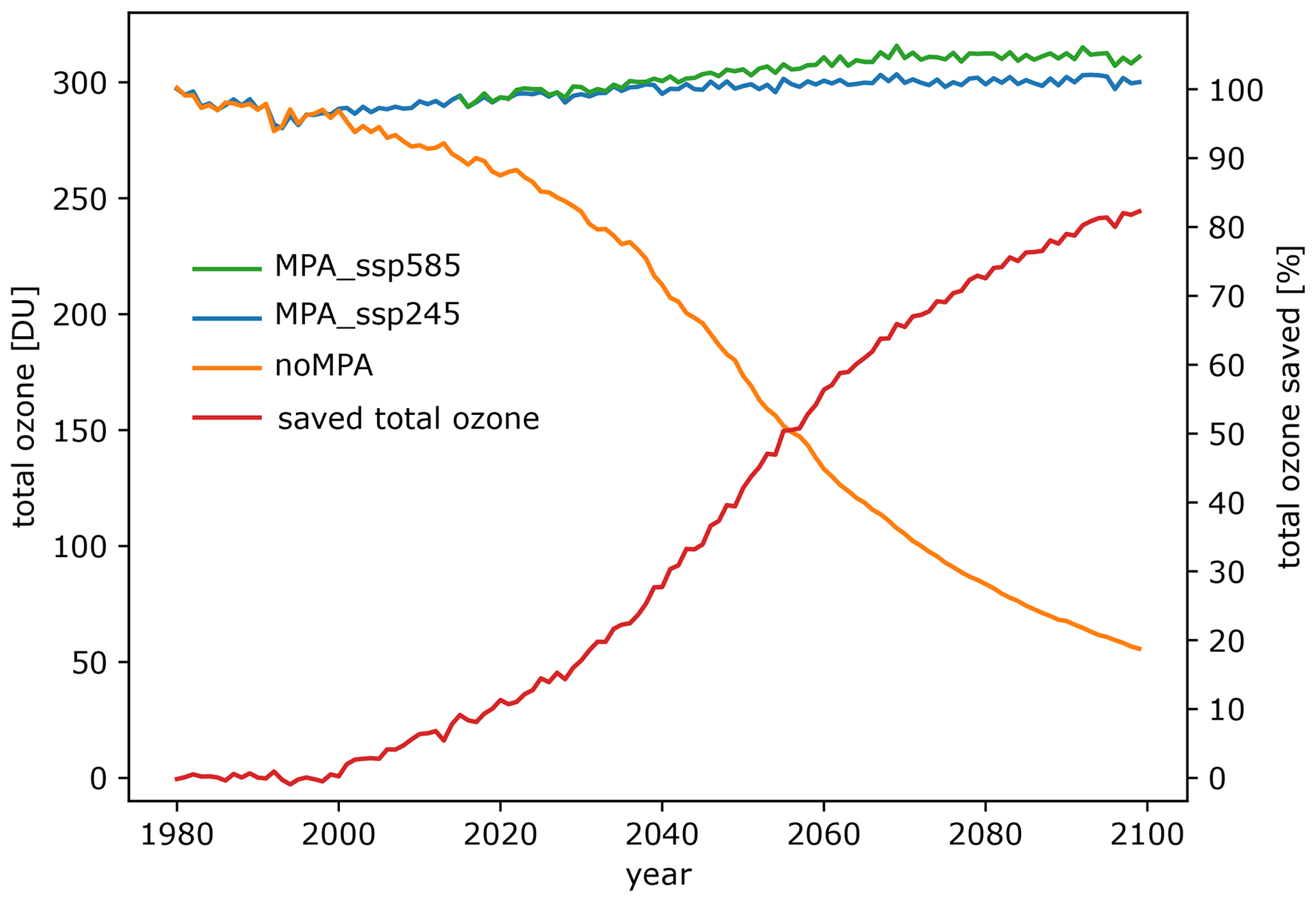
Figure 1 Time evolution of the global-mean annual-mean total ozone (DU, Dobson unit) for the MPA_ssp245 (blue line), MPA_ssp585 (green line), and noMPA (orange line) simulations. The red line illustrates saved total ozone by the MPA limitations (MPA_ssp245-noMPA).

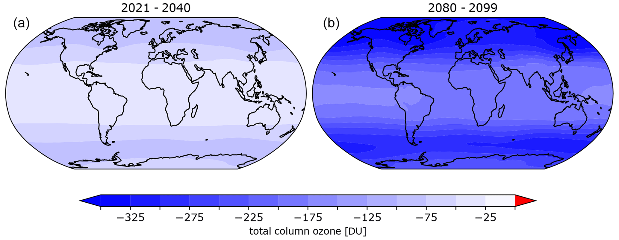
Figure 2 Geographical distribution of the annual-mean total ozone difference (in DU) between noMPA and MPA_ssp245 simulations averaged over the periods (a) 2021–2040 and (b) 2080–2099. All differences are statistically significantly different from 0 at the 90 % level.

Several attempts have been made to estimate the efficacy of the MPA by comparing the future state of the ozone layer simulated under two hypothetical scenarios: with and without MPA limitations. The so-called “world avoided” case (without MPA) is interesting because it allows for an evaluation of the advantages of the Montreal Protocol implementation and helps to further convince society about the necessity of this action (e.g., Newman et al., 2009). Besides this, it represents an interesting extreme sensitivity case for global models, allowing for learning more about the mechanisms of how atmospheric radiation, chemistry, and dynamics are interacting. Each of the past studies, made with models of different levels of complexity and interactivity, have discovered many new details of the avoided atmospheric and climatic effects compared to what had been initially hypothesized when the MPA action was taken. The first estimates were made with relatively simple models (e.g., Prather et al., 1996). Later, Egorova et al. (2001) and recently Chipperfield et al. (2015) performed more accurate estimates using 3-D chemistry-transport models driven by observed meteorological fields. An improved understanding of the influence and importance of ozone on the climate led to the application of chemistry-climate models that can account for stratospheric changes related to the ozone evolution (Morgenstern et al., 2008; Newman et al., 2009; Egorova et al., 2013). The results of these studies confirmed that the absence of MPA limitations would have led to dramatic ozone loss and an increase in the level of dangerous UV radiation near the surface. However, these models have certain limitations for modeling the effect of the restrictive measures of the Montreal Protocol on ozone evolution and climate. For example, in Newman et al. (2009) and Egorova et al. (2013), the use of prescribed sea-surface temperature did not allow for considering tropospheric temperature response to halogen forcing or stratospheric changes. And the lack of troposphere chemistry (Morgenstern et al., 2008; Newman et al., 2009; Egorova et al., 2013) led to incorrect modeling of the tropospheric response with possible implications for the stratosphere. In addition, hODSs are also very potent greenhouse gases (GHGs). They can directly affect radiation balance (e.g., Polvani et al., 2020) in the present-day atmosphere, but in the case of uncontrolled increase in hODSs, their radiative forcing can be comparable to or even exceed the other GHGs (Liang et al., 2022). Therefore, proper evaluation of the MPA influence on climate is not possible without the application of dynamically coupled ocean–atmosphere models. First, Garcia et al. (2012) applied a coupled chemistry–climate–ocean model and showed that, in addition to the collapse of the ozone layer, the uncontrolled growth of hODSs would have caused enhanced global-mean warming from 2010 to 2070 between 2 K, in the tropics and 6 K, in the Arctic; this is comparable to the effects of carbon dioxide increase from 325 to 560 ppmv (IPCC RCP4.5 scenario, Intergovernmental Panel on Climate Change Representative Concentration Pathway) and would have had substantial implications for sea-ice coverage. However, the robustness of these conclusions cannot be established because this experiment had only one run and was not performed with other models. Further, Goyal et al. (2019) tried to increase awareness for the wider community about the MPA's success in climate warming reduction. They used the ACCESS1.0 (Australian Community Climate and Earth-System Simulator v1.0) coupled atmosphere–ocean–land–sea-ice model but without interactive atmospheric chemistry to estimate the impact of MPA on surface temperature warming. In this work, the stratospheric ozone field was prescribed from GEOSCCM (Goddard Earth Observing System Chemistry-Climate Model; Pawson et al., 2008) for a scenario with no MPA and a reference scenario, while the tropospheric ozone concentration was fixed for both experiments. Goyal et al. (2019) showed that for the year 2019 the MPA already prevented additional 0.5–1.0 ^∘C warming over land in middle latitudes (Africa, North America, Eurasia) and in the Arctic. For 2050, they obtained larger MPA effects, reaching 1.5–2.0 ^∘C warming in the extra-polar areas and 3–4 ^∘C in the Arctic with the greenhouse forcing from the RCP8.5 scenario. However, there are various shortcomings in this study. First, the fixed tropospheric ozone approach is difficult to justify for the case with no MPA due to the expected dramatic increase in UV radiation in the troposphere caused by stratospheric ozone depletion and strong tropospheric ozone radiative forcing. Second, the provided results were not supported by statistical significance analysis, and therefore the conclusions about MPA effects in Goyal et al. (2019) require further verification. Morgenstern et al. (2020) obtained larger cooling by ozone depletion than Goyal et al. (2019) and Polvani et al. (2020) and pointed out that the effect of MPA on surface climate would be smaller; therefore there is a need to reduce the uncertainties in the estimation of the MPA regulation effect on surface temperature (Neale et al., 2021). Because of the uncertainties in MPA climate effect estimations, more studies are necessary to clarify and obtain robust results of MPA benefits for Earth's climate. In this paper, we applied the Earth system model (ESM) SOCOLv4.0 (modeling tools for studies of SOlar Climate Ozone Links; Sukhodolov et al., 2021) to simulate the dramatic global-scale depletion of the ozone layer and its consequences on Earth's climate. In Sect. 2 we describe the model, experiment design, and forcing. The results of this study are provided in Sect. 3, followed by the conclusions summarized in Sect. 4.

2 Method

2.1 Model description

The SOCOLv4.0 model used in this study has the standard configuration with horizontal resolutions (T63, approximately 1.9×1.9^∘) and 47 layers in the vertical direction and has been validated against observations and other models using comprehensive statistical tools (Sukhodolov et al., 2021). The model consists of the Earth system model (Max Planck Institute Earth System Model, MPI-ESM, Hamburg, Germany) (Mauritsen et al., 2019), the chemistry (Model for investigating ozone trends, MEZON) (Egorova et al., 2003), and the size-resolving sulfate aerosol microphysics (AER) (Sheng et al., 2015) modules. The chemical module treats more than 100 gas species linked by 216 gas-phase, 72 photolysis, and 16 heterogeneous reactions in/on aqueous sulfuric acid aerosols and polar stratospheric clouds. The photolysis rates are calculated online using the lookup table scheme. All modules are interactively coupled by the 3-D meteorological fields of wind and temperature as well as by the radiative forcing of sulfate aerosol and radiatively active gases including chlorofluorocarbons (CFCs). The model directly simulates many important forcings and feedbacks in the climate system, including oceanic processes and dynamic vegetation. Thus, the model accounts for most of the known atmospheric processes involved in the ozone net chemical production and transport as well as chemistry-dynamics feedbacks. Extensive model validation showed that the climatology and variability in the temperature/circulation fields, as well as the distribution of several key atmospheric tracers, are successfully reproduced (see Sukhodolov et al., 2021, for further details). Despite some differences related to interactive chemistry and aerosol, the representation of several climate parameters such as clouds, precipitation, and sea-ice coverage is very similar to the core MPI-ESM model discussed in Mauritsen et al. (2019).

Figure 3 Zonal, annual, and ensemble mean of the total inorganic chlorine (Cl_y), O₃, NO_x(N+NO+NO₂), OH, H₂O, total reactive nitrogen (NO_y), CH₄, H₂O, N₂O (in %), and temperature (in K) response to the absence of the MPA regulations (noMPA relative to MPA_ssp245) averaged over 2080–2099. All differences are statistically significantly different from 0 at the 90 % level except areas with black dots.

2.2 Experimental design and forcing

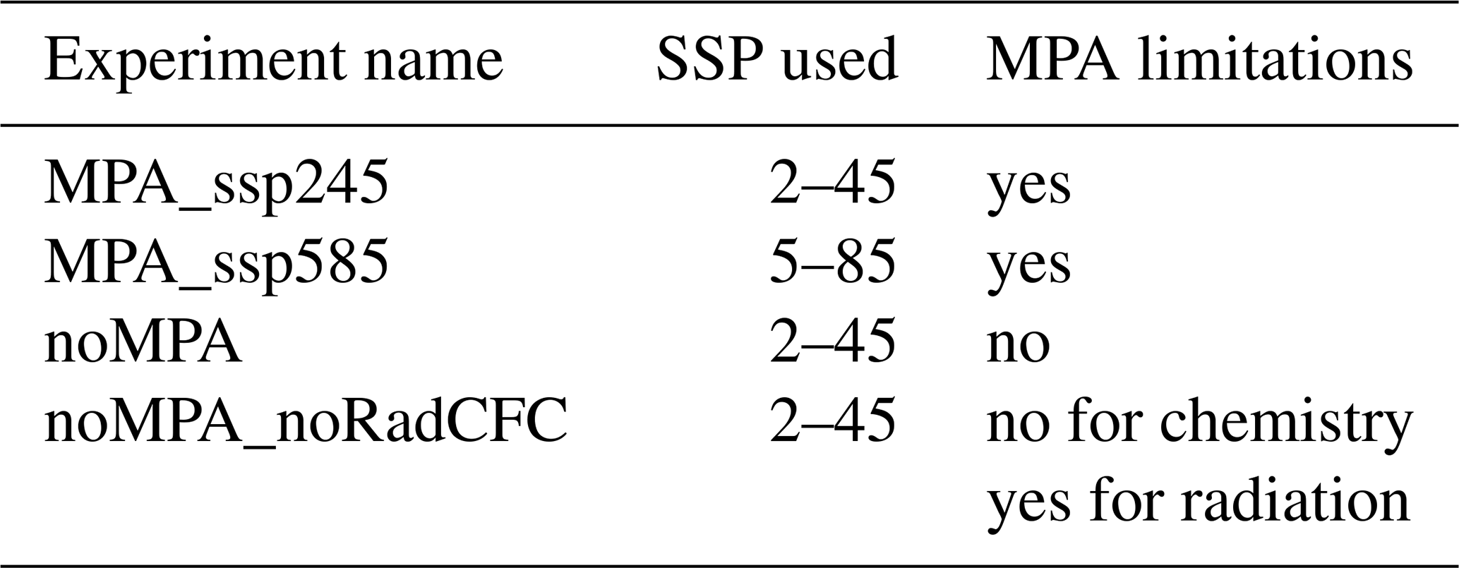
To assess the benefits of the Montreal Protocol and its amendments and adjustments for atmospheric composition and climate, we performed two main three-member 120-year-long (1980–2100) ensemble simulations with SOCOLv4.0 switching on (MPA) and off (noMPA) limitations on the emissions of hODSs. For the model spin-up time we used December 1949 as a restart point from the MPI-ESM 100-year historical experiment (Maher et al., 2019). For the MPA and noMPA cases, the model boundary conditions mostly follow the recommendations of CMIP6 (Coupled Model Intercomparison Project) provided by the input4MIPs database (https://esgf-node.llnl.gov/search/input4mips/, last access: 21 April 2023); this was described in Sukhodolov et al. (2021). All anthropogenic forcing except for hODSs is historical before 2015 and then switched to the SSP2-4.5 (Shared Socioeconomic Pathway) scenarios till 2100, accordingly. The experiment with MPA restrictions under the SSP2-4.5 scenario further will be named MPA_ssp245. For the long- and short-lived halogenated source gases, we used the baseline mixing ratio scenario from WMO (2018), which is a combination of the observation record up to the year 2017 (Engel et al., 2018) and CMIP6 data (Eyring et al., 2016). Several newly discovered and unregulated hODSs (CFC-112, CFC-112a, CFC-113a, CFC-114a, and HCFC-133a) have been introduced to the model chemistry scheme together with some additional chlorine-containing very short-lived substances (VSLSs: CHCl3, CH2Cl2, C2Cl4, C2HCl3, C2H4Cl2) that are not controlled by the MPA (Hossaini et al., 2017). For the noMPA experiment, we applied the same boundary conditions except for the hODSs, whose surface mixing ratio was increased by 3 % yr⁻¹ since 1987 (Velders et al., 2007) for regulated species. For unregulated species we follow the recommendations of WMO (2018): from 2016 CFC-112a grows 1.5 % yr⁻¹, CFC-113a grows 6.5 % yr⁻¹, and HCFC-133a grows 5.4 % yr⁻¹. HCFC-141b, CH3Cl, CHBr3, CH2Br2, and H-2402 are assumed to be equal to the reference case value. In addition to the main two experiments, we performed a run with the MPA limitations using the SSP5-8.5 scenario (MPA_ssp585) to compare climate effects with the MPA_ssp245 experiment. To distinguish between the ozone and direct greenhouse effects of CFCs, we performed a model run, where increasing CFCs were active only chemically but not radiatively under the SSP2-4.5 scenario (noMPA_noRadCFC). The statistical significance of all results shown in the following sections has been calculated using a two-sided t test with a 90 % significance level.

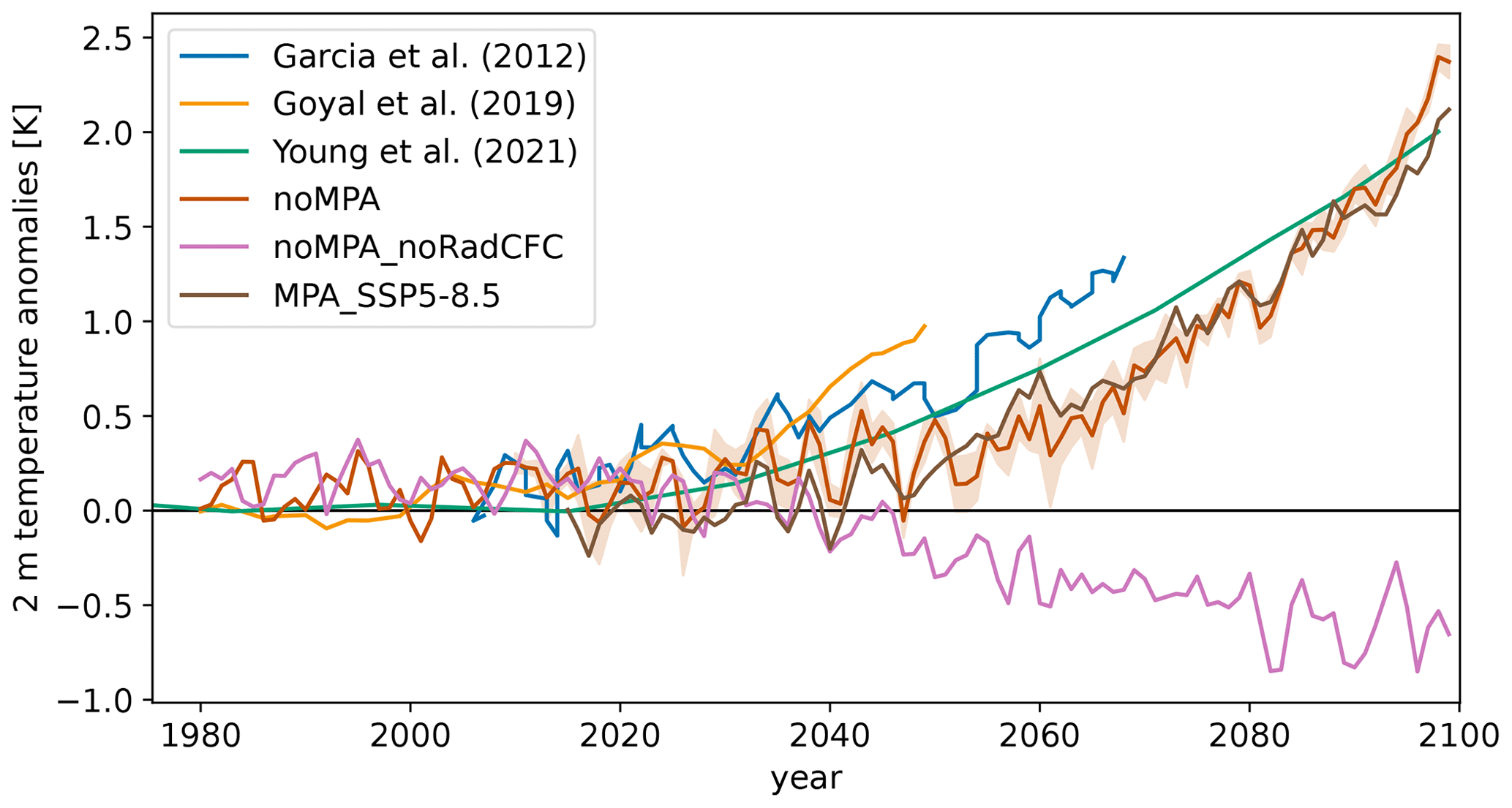
Figure 4 Global-mean surface air temperature deviation for the noMPA (red line), MPA_ssp585 (brown line), and noMPA_noRadCFC (violet line) from the reference MPA_ssp245 run. A light-red shadow illustrates internal variability in the noMPA run. For comparisons, the same quantity is shown using digitized data from Garcia et al. (2012, blue line), Goyal et al. (2019, yellow line), and Young et al. (2021, light-green line).

Table 1 Model experiments.

3 Results and discussion

3.1 MPA benefits for the total column ozone

Figure 1 shows the global, annual, and ensemble mean total ozone from the MPA_ssp245, MPA_ssp585, and noMPA experiments simulated with SOCOLv4 and the amount of saved total ozone by MPA, calculated as the absolute difference between the MPA_ssp245 and noMPA experiments. Without MPA, ozone could be almost entirely depleted by the end of the 21st century, and this result agrees very well with previous publications (e.g., Newman et al., 2009; Garcia et al., 2012; Egorova et al., 2013). The model results demonstrate that the continuous increase in stratospheric halogens destroys about 80 % of the total ozone at the end of the 21st century, and it is difficult to overemphasize the importance of the MPA for preserving the ozone layer. Besides the direct consequences for human health, the increased surface UV radiation would also strongly affect the terrestrial and aquatic ecosystems (Neale et al., 2021) and biogeochemical cycles (Young et al., 2021).

Figure 2 shows the geographical distribution of annual and ensemble mean total ozone changes due to the absence of MPA regulations for the time periods 2021–2040 and 2080–2099. The most pronounced changes take place over the northern high latitudes and middle latitudes of both hemispheres, where halogen chemistry is the most active. It is interesting to note that the southern polar area is less sensitive. It is explained by already large ozone depletion caused by the present-day hODS level, leading to slight saturation of the effects. As expected, smaller but still considerable changes occur over the tropical latitudes where the ozone layer is still maintained to some extent by the in situ production through photolysis of molecular oxygen. All obtained results are statistically significant even for the near-present time period of 2021–2040, which means that in a world with no MPA some dramatic consequences could already be observable.

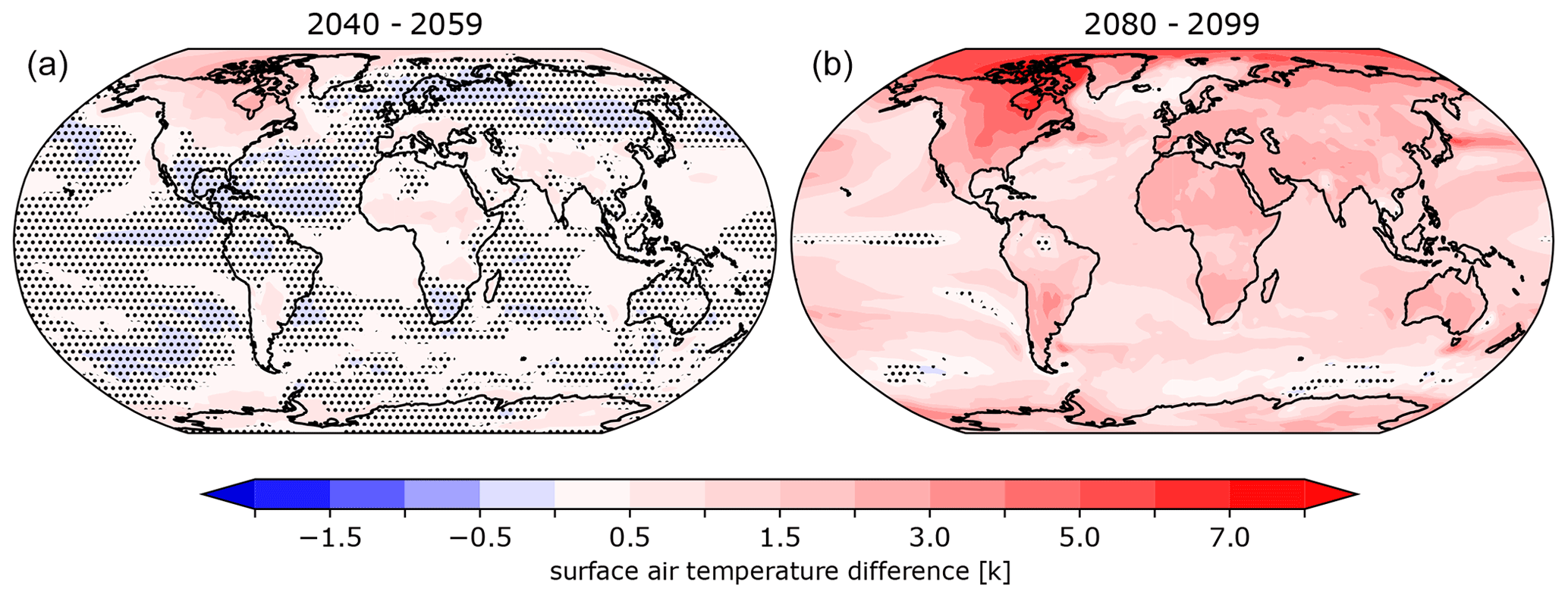
Figure 5 Geographical distribution of annual-mean difference in the surface air temperature between noMPA and MPA_ssp245 simulations averaged over the periods 2040–2059 and 2080–2099 (in K). Areas where the statistical significance of the signal is less than 90 % are marked by dots.

3.2 Chemical composition and temperature changes

It is of interest to analyze the impact of hODSs on chemical composition and temperature because it helps to understand the response of the ozone and climate. Moreover, for the extreme conditions that the atmosphere would be put in, the luckily avoided noMPA scenario presents an interesting exercise that allows us to provide new insights into the chemical and dynamic links in the atmosphere–climate system. Figure 3 shows the response of several essential chemical species and temperature to the absence of MPA limitations for the 2080–2099 period. An uncontrolled increase in the hODS emissions dramatically (around 2000 %) enhances Cl_y concentration. This primary forcing leads to ozone depletion in most of the stratosphere. The ozone decrease maximizes in the upper and lower stratosphere. In the upper stratosphere, the efficiency of gas-phase chlorine-based catalytic ozone destruction cycles is the highest (e.g., Revell et al., 2012). In the lower stratosphere, almost complete ozone depletion similar to the finding of Newman et al. (2009) is explained by the acceleration of heterogeneous chlorine activation, which is caused by the cooling in this area. The cooling accelerates heterogeneous reactions and enhances surface area density (SAD) due to the additional generation of the liquid sulfate aerosol in the Junge layer (Junge and Mandson, 1961) and the appearance of the polar stratospheric clouds (PSCs). The obtained increase in annual-mean SAD in the noMPA run relative to the reference exceeds 100 % in the entire lower stratosphere, except for southern high latitudes (not shown). Lower SAD in this area is explained by a substantial decrease in type I PSCs due to HNO₃ depletion caused by enhanced chlorine loading. In the tropical lower stratosphere (10–20 km), the model shows about a 20 % ozone increase caused by the increase in the oxygen photolysis rates in the lower stratosphere related to strong ozone depletion higher up leading to a downward shift in the net ozone production. The obtained pattern of the ozone response is very close to the other model results (e.g., Morgenstern et al., 200; Newman et al., 2009).

The ozone abundance is tightly related to atmospheric chemistry due to the modulation of the temperature structure and photolysis rates. Well-pronounced cooling in the stratosphere is mostly related to ozone depletion and reaches maxima in the upper stratosphere where the ozone absorption of solar UV radiation is the main energy source. The secondary maximum cooling in the lower stratosphere is formed by both ozone depletion and intensification of the Brewer–Dobson circulation (e.g., Zubov et al., 2013) caused by the tropospheric warming owed to the direct radiative forcing of hODSs as well as by the modulation of the temperature gradients in the stratosphere. The tropical pattern of the temperature response is similar to the Garcia et al. (2012) and Newman et al. (2009) results. More details of climate warming will be discussed in Sect. 3.3. Tropospheric warming is responsible for the increase in tropospheric water vapor mostly because warmer air can hold more water vapor according to Clausius–Clapeyron law and partially due to enhanced evaporation from the warmer surface.

Together with enhanced ozone photolysis followed by more intensive O(¹D) production, it leads to substantially higher (up to 100 %) hydroxyl concentration, with a negative impact on tropospheric ozone that is also lowered because of the reduced transport from the stratosphere. The stratospheric water vapor slightly decreases in the upper stratosphere, where the methane oxidation cycle is still operational. However, in the lower stratosphere, where the influx from the troposphere dominates, the water vapor concentration drops by up to 70 % due to a cooler environment and a more efficient cold trap at the entry level. This process and lower ozone concentration (less O(¹D)) suppresses hydroxyl radical production and decreases the stratospheric oxidation capacity. A substantial amount of HO_x is also removed via HO₂+ ClO = HOCl + O₂ due to very high chlorine loading. The effect of a lower OH mixing ratio is more visible in the weaker ozone depletion in the lower mesosphere and partially in the tropical lower stratosphere. The major source gases such as methane and N₂O demonstrate rather similar behavior, with very weak changes in the troposphere and substantial depletion above approximately 30 km. The methane decrease in the troposphere is caused by enhanced hydroxyl concentration. Above 30 km, methane is being destroyed by atomic chlorine via the reaction CH₄+ Cl = HCl + CH₃. Tropospheric N₂O is not extensively sensitive to other species and photolysis rates, so it only very weakly reacts to the introduced forcing. Two spots of positive N₂O changes over the extratropics are probably formed due to the deficit of the O(¹D) related to ozone depletion. N₂O decrease above 25 km is most likely related to the enhanced photolysis (N₂O+ hv = N₂ + O), which does not enhance NO_y production. As a result, NO_y concentration drops in the entire stratosphere because of enhanced NO photolysis followed by the cannibalistic reaction NO + N = N₂ + O in combination with a substantial N₂O decrease. Reactive NO_x radical depletion is even more intensive than NO_y. It can be explained by the conversion to ClONO₂ (via NO₂ + ClO = ClONO₂) in the high-chlorine-loading atmosphere. NO_y increase in the tropical upper troposphere is partly related to the enhanced lightning flash frequency and convective activity in the warmer climate (e.g., Mareev and Volodin, 2014; Revell et al., 2015). The obtained results show that an uncontrolled increase in halogen loading affects chemical processes and the temperature distribution in the entire atmosphere from the ground to the mesosphere.

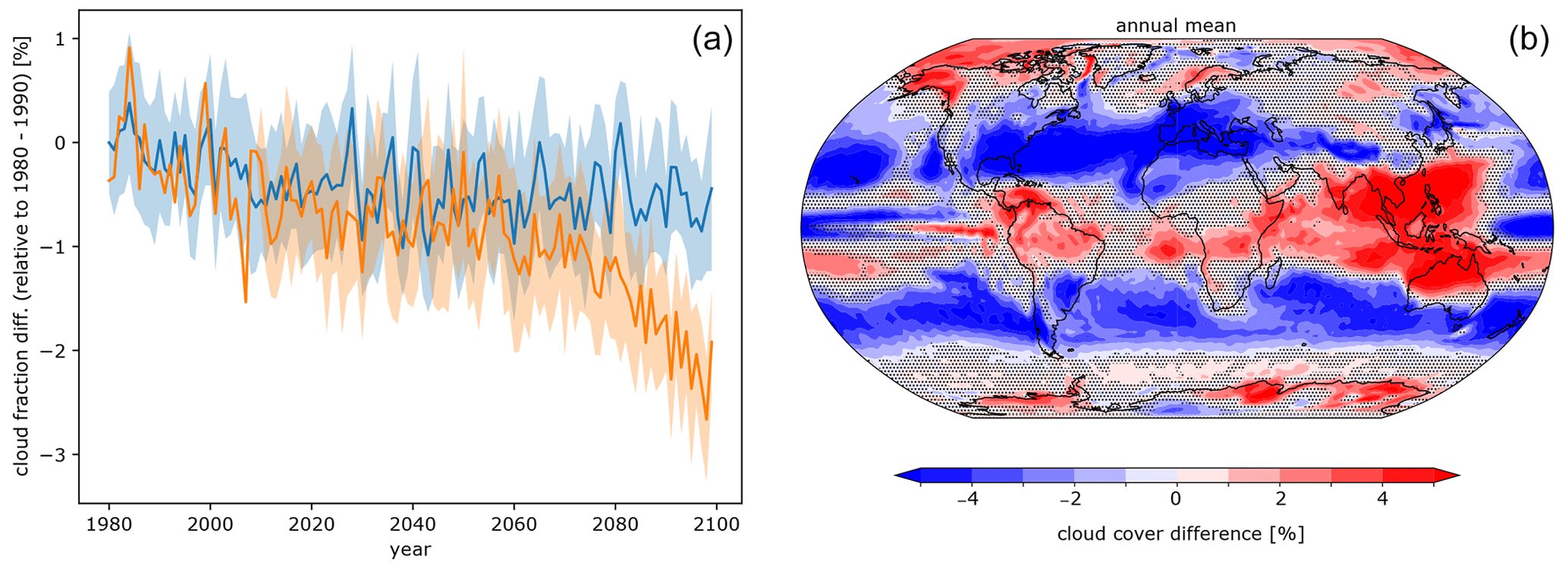
Figure 6 (a) Time evolution of global and annual-mean cloud cover change for MPA_ssp245 (blue) and for noMPA (orange) cases relative to the 1980–1990 mean and (b) geographical distribution of the annual-mean difference in cloud cover (%) between noMPA and MPA_ssp245 simulations averaged over the period 2090–2100. Areas where the statistical significance of the signal is less than 90 % are marked by dots.

3.3 MPA implications for the surface air temperature

As was mentioned above, the troposphere would warm by up to 3 K without MPA restrictions at the end of the 21st century (see Fig. 3). It means that the MPA not only protects the ozone layer but also helps to limit greenhouse warming (Velders et al., 2007) as described in IPCC (2013). Here, we analyze surface air temperature in more detail to illustrate the benefits of the MPA limitations for the surface climate. Figure 4 shows the time evolution of global-mean temperature response for all considered cases in comparison with the other model results published by Garcia et al. (2012), Goyal et al. (2019), and Young et al. (2021). Garcia et al. (2012) exploited the Whole Atmosphere Community Climate Model with interactive chemistry coupled to a deep-ocean model and the IPCC RCP4.5 scenario for greenhouse gas (GHG) emissions. The Australian Community Climate and Earth-System Simulator v1.0 (ACCESS1.0), which is a coupled atmosphere–ocean–land–sea-ice model without interactive chemistry, was applied by Goyal et al. (2019) to simulate the atmospheric state using the IPCC RCP8.5 scenario for GHGs with and without MPA. Young et al. (2021) simulated climate using the NIWA–UKCA (New Zealand National Institute of Water and Atmospheric Research–United Kingdom Chemistry and Aerosols) chemistry–ocean–climate model in combination with a land surface model driven by the IPCC RCP6.0 scenario for GHGs and also with and without MPA limitations. Figure 4 demonstrates the difference between noMPA and reference runs, which does not dramatically depend on the basic scenario. Before approximately 2030, all models show a slightly (within 0.25 K) warmer climate. Then the warming starts to grow at a higher rate for Garcia et al. (2012), Goyal et al. (2019), and Young et al. (2021). Our model demonstrates weaker warming until approximately 2060 and a sharp temperature increase during the second half of the century. In 2100 the warming from our model is even higher than in Young et al. (2021). This disagreement looks statistically significant, but the reason is not easy to understand. The model's peculiarities could play a role. It is known (e.g., IPCC, 2013) that climate sensitivities are not in perfect agreement among the models. The ocean inertia could also strongly affect the magnitude of the response. Another aspect is related to the treatment of the hODS distribution. In climate models without interactive chemistry, hODSs are usually prescribed as a single value for the entire atmosphere. In the chemistry-climate models, there is the possibility of doing the same or utilizing 3-D hODS concentration from the chemical module for calculating radiation fluxes and heating rates. Due to intensive destruction by solar UV radiation, hODSs almost disappear from the stratosphere, which diminishes their radiative forcing. This process is insignificant for the hODS concentration close to the present-day values but becomes more important in the future for the noMPA case. It can explain a smaller temperature response in our model in comparison with the prescribed chemistry model of Goyal et al. (2019). Still, the reason for the difference with results from Garcia et al. (2012) remains unclear because we do not know how hODSs were treated in their model.

An interesting fact to note is that the noMPA case gives virtually the same global warming rate as the MPA_ssp885, which emphasizes the importance of MPA for global climate. The influence of the ozone change is also shown in Fig. 4. For the noMPA_noRadCFC run, uncontrolled hODS increase was applied only for the chemical module, while infrared radiative forcing from hODSs was kept as in the reference (MPA_ssp245) case. The ozone depletion discussed earlier in Sect. 3.2 caused significant global cooling by up to 0.8 K. This can be explained mainly by the decrease in ozone in the troposphere and stratosphere (see Fig. 3), where it has a strong radiative forcing potential. The separation of these two physical processes requires several additional experiments and cannot be done in the present paper framework.

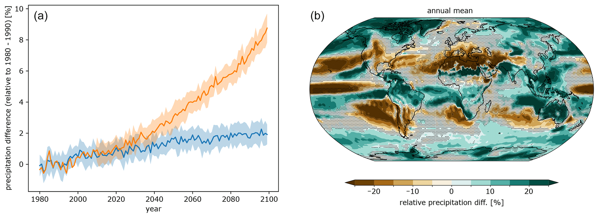
Figure 7 (a) Time evolution of global-mean and annual-mean precipitation change for reference MPA_ssp245 (blue) and for noMPA (orange) cases relative to the 1980–1990 mean and (b) geographical distribution of the annual-mean difference in precipitation between noMPA and MPA_ssp245 simulations averaged over the period 2090–2100 (in %). Areas where the statistical significance of the signal is less than 90 % are marked by dots.

Figure 5 shows the regional effects of MPA regulations on surface air temperature for annual-mean values for two periods. Uncontrolled hODS increase leads by the end of the 21st century to robust warming all around the globe. The pattern of the warming is typical of the warmer climate (IPCC, 2013) with up to 8 K warming in the northern high latitudes, reflecting well-known Arctic amplification (e.g., Prevedi et al., 2021). In general, the warming maximizes over the land masses and is only about 1 K over the oceans. The smaller warming, as in the case of GHG increase (e.g., IPCC, 2013), is visible over the northern Atlantic. The temperature response is insignificant during the 2020–2040 period (not shown) and starts to appear over North America, the Arctic, Asia, and Africa only after 2040. Small and even not robust warming just after 2020 does not agree with the results of Goyal et al. (2019), who demonstrate substantial warming already during the early 21st century. It looks reasonable due to their larger global-mean response (see Fig. 4). However, their results are also difficult to interpret because Goyal et al. (2019) did not provide statistical significance of the results and internal variability in the climate system can provide quite substantial noise even with five ensemble members.

3.4 MPA impact on cloud cover, precipitation, and sea ice

Among essential climate variables, cloud amount and precipitation intensity play an important role because they demonstrate energy and water flux changes in the climate system, which are dramatically important for the environment (e.g., IPCC, 2013). Figure 6 (left panel) illustrates the evolution of the global- and annual-mean cloud cover for the MPA (reference) and noMPA cases relative to the 1980–1990 period. The cloud amount response is small (within 1 %) until approximately 2060 for both cases, and the difference between cases is not statistically significant. After 2060, the global-mean cloud amount decrease due to the absence of the MPA limitations is observable, reaching about 2 % at the end of the century, and is more pronounced than in the reference case. The small global-mean response could be related to the redistribution of the cloud field caused by the circulation changes in the warmer climate. The geographical distribution of the cloud amount supports this explanation, showing a very inhomogeneous pattern. The cloud amount increase over the high and tropical latitudes competes with a pronounced decrease over the extratropics, leading to very small changes (up to 2 % at the end of the 21st century) in the global mean. The obtained pattern resembles the results of climate models obtained for the RCP8.5 scenario (see Fig. 12.17 of IPCC, 2013), but there are some deviations in the Maritime Continent, South America, Australia, and southern Africa, where the cloud response to hODS forcing has a different sign. It should be noted, however, that these differences could rather be related to our model peculiarities.

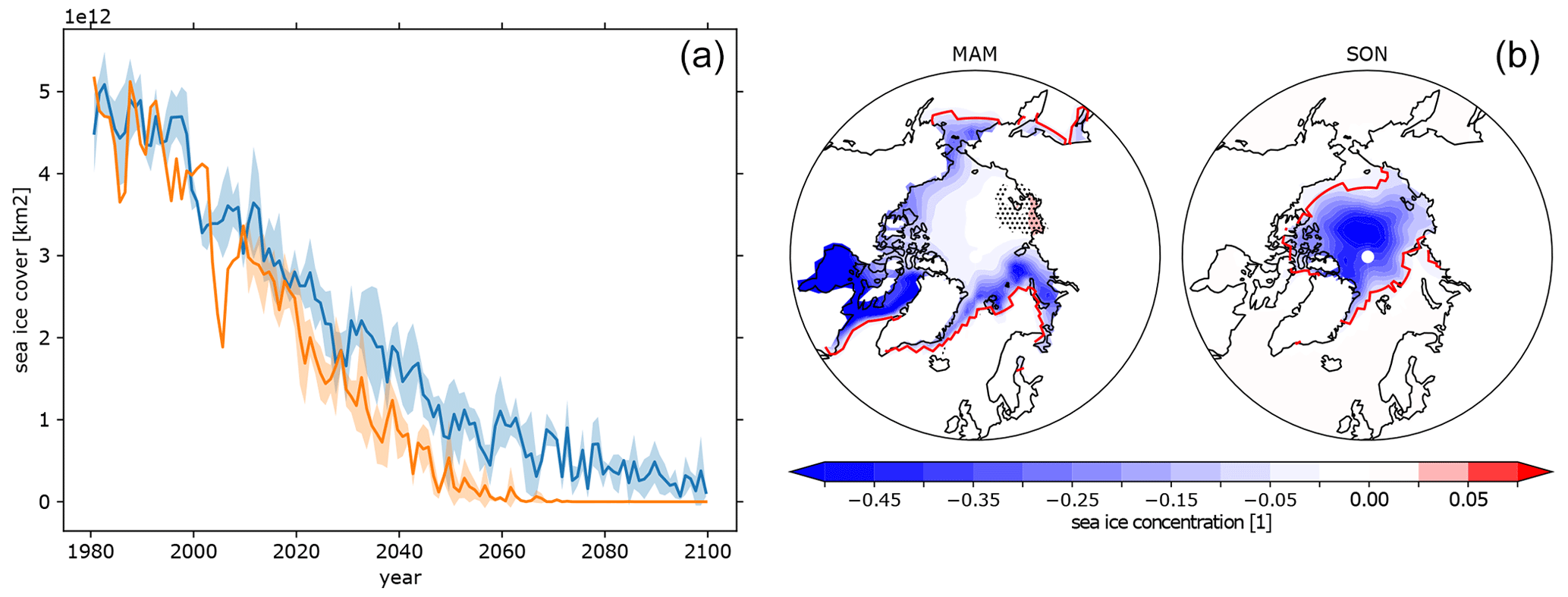
Figure 8 (a) September sea-ice extent time evolution for reference MPA_ssp245 (blue) and for no MPA (orange) cases. (b) Sea-ice loss due to hODSs for 2080–2099; the red line represents sea-ice extent of the reference MPA_ssp245 run. MAM: March–April–May, SON: September–October–November.

Figure 7 shows substantial changes (up to 9 % at the end of the 21st century) in global-mean precipitation and its spatial distribution. In a warmer climate, we expect more water vapor in the atmosphere and consequently substantial changes in precipitation intensity. It is known (IPCC, 2013, 2022) that the global-mean precipitation increases in a warming climate. The rate is not perfectly constrained and can be within 1 %–4 % per 1 K warming. In our case, we have about 2 K warming for the noMPA case (see Fig. 4) and a consistent extra 7 % precipitation amount. As expected, the geographical distribution of the precipitation changes resembles the cloud cover response.

High-latitude areas, the tropical belt, Australia, and the Maritime Continent experience a substantial (more than 20 %), statistically significant precipitation increase. Greater changes over the high latitudes are explained by increased water vapor transport from the tropical latitudes (IPCC, 2013). The Mediterranean region becomes substantially (by up to 20 %) drier, responding to the absence of MPA limitations. Over the Pacific Ocean, the pattern is not homogeneous. The obtained precipitation changes resemble the results presented in IPCC (2022, Fig. 4.24) but are not identical. Our model produces very different precipitation changes over Australia and southern Africa. However, the magnitude of the changes due to the absence of MPA limitations is comparable with the precipitation response obtained for the SSP3-7.0 scenario (IPCC, 2022).

The status of the North Sea ice cover is essential for the Arctic biosphere as well as for the economic issues related to transportation, tourism, population life, and fossil fuel extraction (e.g., Notz et al., 2016). All these factors make sea ice one of the main climate indicators. As shown above, in Fig. 5, the Arctic region experiences large warming if the MPA had not been implemented. The implications on the September sea-ice cover are visible in Fig. 8 (left panel). The Arctic would be ice-free (cover less than 1×10⁶ km²) in September around 40 years earlier, i.e., around 2050 without MPA compared to 2090 with MPA. A similar early timing of an ice-free Arctic is also seen for simulations with the SSP5-8.5 scenario (see for example Fig. 4.2c of the IPCC AR6 in Lee et al., 2021). The minimum sea-ice cover is decreased on the whole surface quite uniformly (right panel of Fig. 8). In spring, however, which is the time of the maximum sea-ice extension, the reduction is confined to the edge of the sea-ice cover. Hudson Bay and Baffin Bay would be largely ice-free at the end of the century without the MPA. Additionally, the sea-ice edge between Svalbard and Siberia moves to the north, and Fram Strait has a reduced cover, leading to the conclusion that there is less transport of sea ice out of the Arctic Basin.

4 Summary and conclusions

This paper describes the climate and atmosphere benefits of the MPA simulated with the Earth system model SOCOLv4.0 using the CMIP6 boundary conditions and Socioeconomic Pathway scenarios. We have added to and confirmed the previous studies by showing that, without the MPA by the end of the 21st century, there would be a dramatic reduction in the ozone layer as well as a huge perturbation of the essential climate variables in the troposphere caused by the warming from increasing hODSs.

With the performed simulations, we have confirmed the value and benefits of MPA limitations for the ozone layer and climate, considering multiple feedbacks within the Earth system. The uncontrolled increase in hODSs influences the chemical processes and temperature distribution in the entire atmosphere from the surface to the mesosphere. Ozone could be almost entirely depleted, and surface temperature could be warmer all around the globe and up to 8 K in the northern high latitudes, reflecting well-known Arctic amplification. Also, cloud cover and precipitation would be affected. Our simulations with ESM SOCOLv4 showed very small changes in global-mean cloud amount, by about a 2 % decrease at the end of the century due to the competing between an increase over the high and tropical latitudes and a pronounced decrease over the extratropics, and the geographical distribution of the precipitation changes resemble the cloud cover response. The modeling results for the sea ice show that the Arctic would be ice-free around 40 years earlier, i.e., around 2050 without MPA compared to 2090 with MPA.

The warming rate of the noMPA scenario under the SSP2-4.5 conditions would be very similar to that from the SSP5-8.5 conditions with MPA; i.e., the harsh future without MPA would combine both the negative health effects from the increased UV radiation at the surface and most of the negative consequences of the high-end future climate pathway described in detail by IPCC (2021). Such a combination of fast and strong negative environmental changes would trigger further socioeconomic problems like shortages of food and water insecurity (Barnes et al., 2019), unprecedented migration (Ionesco et al., 2016), and civil and international conflicts (e.g., Hsiang et al., 2011), with many of the negative effects starting to emerge already in the current decade.

Our paper reminds us again how timely and extremely important the MPA was. The Montreal Protocol is one of the few cases in human history when all countries urgently agreed on measures benefiting the survival of humanity. The ozone layer made life on terrestrial land possible (e.g., Ratner and Walker, 1972), and we were very close to severely damaging it. The Montreal Protocol science should continue to be conveyed in the future to remind society how vulnerable and close to a total disaster we could be and that international dialogue and consensual decisions on environmental questions are possible.