The response of the North Pacific jet and stratosphere-to-troposphere transport of ozone over western North America to RCP8.5 climate forcing

Stratosphere-to-troposphere transport (STT) is an important source of ozone for the troposphere, particularly over western North America. STT in this region is predominantly controlled by a combination of the variability and location of the Pacific jet stream and the amount of ozone in the lower stratosphere, two factors which are likely to change if greenhouse gas concentrations continue to increase. Here we use Whole Atmosphere Community Climate Model experiments with a tracer of stratospheric ozone (O3S) to study how end-of-the-century Representative Concentration Pathway (RCP) 8.5 sea surface temperatures (SSTs) and greenhouse gases (GHGs), in isolation and in combination, influence STT of ozone over western North America relative to a preindustrial control background state.

We find that O3S increases by up to 37 % during late winter at 700 hPa over western North America in response to RCP8.5 forcing, with the increases tapering off somewhat during spring and summer. When this response to RCP8.5 greenhouse gas forcing is decomposed into the contributions made by future SSTs alone versus future GHGs alone, the latter are found to be primarily responsible for these O3S changes. Both the future SSTs alone and the future GHGs alone accelerate the Brewer–Dobson circulation, which modifies extratropical lower-stratospheric ozone mixing ratios. While the future GHGs alone promote a more zonally symmetric lower-stratospheric ozone change due to enhanced ozone production and some transport, the future SSTs alone increase lower-stratospheric ozone predominantly over the North Pacific via transport associated with a stationary planetary-scale wave. Ozone accumulates in the trough of this anomalous wave and is reduced over the wave's ridges, illustrating that the composition of the lower-stratospheric ozone reservoir in the future is dependent on the phase and position of the stationary planetary-scale wave response to future SSTs alone, in addition to the poleward mass transport provided by the accelerated Brewer–Dobson circulation. Further, the future SSTs alone account for most changes to the large-scale circulation in the troposphere and stratosphere compared to the effect of future GHGs alone. These changes include modifying the position and speed of the future North Pacific jet, lifting the tropopause, accelerating both the Brewer–Dobson circulation's shallow and deep branches, and enhancing two-way isentropic mixing in the stratosphere.

1 Introduction

Tropospheric ozone is a pollutant harmful to humans and vegetation; therefore, understanding its response to climate change has important implications for future air quality (Fleming et al., 2018; Zanis et al., 2022). Future tropospheric ozone amounts are affected by multiple processes, including anthropogenic emissions and changes to the large-scale circulation, which in turn are dependent on the choice of model and climate change scenario (Young et al., 2018). For high-end emissions scenarios (Representative Concentration Pathway (RCP) 8.5), recent chemistry–climate models project an increase in Northern Hemisphere tropospheric ozone (Archibald et al., 2020), largely due to enhanced methane emissions (Winterstein et al., 2019) but also due to stronger transport of stratospheric ozone into the troposphere (Griffiths et al., 2021).

Enhanced stratosphere-to-troposphere transport (STT) of ozone is expected in the future, due in part to more frequent tropopause folding (Akritidis et al., 2019) but also due to higher ozone mixing ratios in the lower stratosphere. Since the amount of ozone in the lower extratropical stratospheric “reservoir”, often measured on the 350 K isentrope, is positively correlated with the amount of ozone contained in intrusions of stratospheric air exchanged into the troposphere (Albers et al., 2018), larger lower-stratospheric ozone mixing ratios should coincide with more STT of ozone. A diverse set of physical and chemical processes is anticipated to have the net effect of increasing future lower-stratospheric ozone mixing ratios in the extratropics; these processes include enhanced downwelling associated with the acceleration of the Brewer–Dobson circulation (BDC) (Abalos et al., 2020), two-way isentropic mixing (Eichinger et al., 2019; Ball et al., 2020; Dietmüller et al., 2021), enhanced ozone production associated with stratospheric cooling (Rind et al., 1990; Jonsson et al., 2004; Oman et al., 2010), chemical impacts of increasing methane and nitrous oxide concentrations (Revell et al., 2012; Butler et al., 2016; Winterstein et al., 2019), and expected emissions reductions of ozone-depleting substances (ODSs) (Banerjee et al., 2016; Meul et al., 2018; Fang et al., 2019; Griffiths et al., 2020; Dietmüller et al., 2021).

While the mechanisms influencing future lower-stratospheric ozone changes are fairly well established in a zonally averaged sense, it is less evident what role regional dynamical and chemical zonal asymmetries will play in future STT. Historically, one of the key regions where stratospheric mass fluxes enter the lower free troposphere is over western North America (Sprenger and Wernli 2003; Lefohn et al., 2011; Škerlak et al., 2014). Tropopause folding and STT maximize over this region during spring, when the North Pacific jet transitions from a strong and latitudinally narrow band of westerlies to a weaker and latitudinally broad jet (Newman and Sardeshmukh, 1998; Breeden et al., 2021). Intrusions here have been observed to enhance free tropospheric ozone concentrations beyond 30 ppb (Knowland et al., 2017; Langford et al., 2017; Zhang et al., 2020; Xiong et al., 2022; Langford et al., 2022). When combined with background ozone concentrations, which are also affected by regional precursor emissions, vegetation, and upwind transport (Cooper et al., 2010; Langford et al., 2017), ozone concentrations may exceed the surface 8 h National Ambient Air Quality Standard (EPA, 2006).

It is established that the subtropical and eddy-driven jets' response to climate change will vary by region and season (Akritidis et al., 2019; Harvey et al., 2020). However, it is not yet known how regional jet changes, such as the spring transition of the North Pacific jet, combined with changes to the lower-stratospheric ozone reservoir may affect STT regionally in the future. In this study, we use a set of National Center for Atmospheric Research (NCAR) Whole Atmosphere Community Climate Model (WACCM) experiments described in Sect. 2, which include fully interactive chemistry and a tracer of stratospheric ozone (O3S), to evaluate how RCP8.5 sea surface temperatures (SSTs) alone and RCP8.5 greenhouse gases (GHGs) alone, and also in combination, influence STT of ozone over western North America. Strictly speaking, warming SSTs in high-emission scenarios such as RCP8.5 result from the increased GHG emissions. However, when considered independently of each other (by holding one fixed while changing the other), the SSTs alone and the GHGs alone have distinct impacts on the future atmosphere, with the SSTs alone being disproportionately responsible for future subtropical jet changes and amplification of the BDC's shallow branch (Oberländer et al., 2013; Chrysanthou et al., 2020) and the GHGs alone being primarily responsible for production of stratospheric ozone and amplification of the BDC's deep branch (Winterstein et al., 2019; Abalos et al., 2021; Dietmüller et al., 2021). Therefore, as is shown in Sect. 3, each forcing, either dynamically or chemically, influences processes that affect STT over western North America. Section 4 synthesizes the results, namely that the RCP8.5 GHGs alone are primarily responsible for future increases in lower-tropospheric O3S over western North America despite the RCP8.5 SSTs alone disproportionately accounting for future dynamical changes in the troposphere and stratosphere, including those associated with the North Pacific jet's spring transition.

2 Methods

We compare output from three different 60-year integrations using NCAR WACCM (Table 1). The version of WACCM used in this study uses a horizontal resolution of 1.9^∘ latitude by 2.5^∘ longitude with 70 vertical layers and a model top near 140 km (Mills et al., 2017; Richter et al., 2017). These experiments do not include an internally generated or prescribed quasi-biennial oscillation; the climatological tropical stratospheric winds are weakly easterly. WACCM has fully interactive chemistry in the middle atmosphere using the Model for Ozone And Related chemical Tracers (MOZART3) and a limited representation of tropospheric chemistry (Kinnison et al., 2007). The chemistry module in WACCM includes a stratospheric ozone tracer (O3S), which is used to quantify STT of ozone. O3S is set equal to the fully interactive stratospheric ozone at each model time step. Once it crosses the tropopause, O3S decays at the tropospheric chemistry rate and is lost due to dry deposition. O3S represents an upper bound on the contribution of the stratosphere to tropospheric ozone, in large part because it is missing some tropospheric chemistry that would likely reduce its lifetime.

To isolate the signal of atmospheric tracers to external forcings above the “noise” of internal atmospheric variability, we have run “time-slice” simulations forced by fixed SSTs, allowing us to both generate longer simulations than more computationally expensive coupled atmosphere–ocean simulations and remove year-to-year fluctuations in ocean sea surface temperatures that may arise internally. Each time-slice simulation has been run for 60 years, with 10 years of spin-up (which is sufficient for initialized atmosphere-only runs).

Table 1 Each experiment is prescribed with fixed repeating annual cycles of the time-averaged SST from the years listed in column three. Greenhouse gas mixing ratios coinciding with the years indicated in column four are shown for four of the species in columns five through eight.

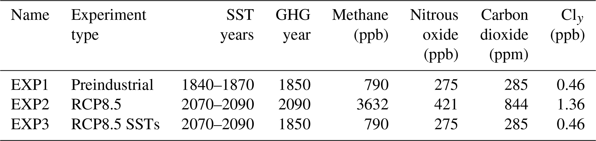
The first experiment (EXP1) is a preindustrial control simulation forced with the year 1850 GHGs and a fixed repeating annual cycle of SSTs and sea ice created from the time-averaged 1840–1870 period. The second experiment (EXP2) is forced with a fixed repeating annual cycle of SSTs and sea ice based on the time-averaged 2070–2090 period from a fully coupled run of the same version of WACCM and GHG concentrations at the year 2090 from the RCP8.5 scenario. The RCP8.5 scenario represents a “worst-case” future scenario in which the radiative forcing imbalance between year 2100 and 1850 is 8.5 W m⁻² due to marked increases in concentrations of carbon dioxide, nitrous oxide, and methane by the end of the century (van Vuuren et al., 2011). We chose this extreme scenario in order to simulate the “upper bounds” of the response. There are also increased concentrations of ozone-depleting substances (ODSs; e.g., chlorofluorocarbons) relative to the preindustrial experiment, due to the long lifetimes of these substances, which were emitted prior to the Montreal Protocol. Non-methane ozone precursor emissions, the solar flux, and stratospheric aerosol concentrations are held fixed to levels of the year 1850. The difference between EXP2 and EXP1 includes the atmospheric response to higher GHGs, more ODSs, and warmer SSTs.

One additional experiment is used to disentangle the atmospheric response to future GHGs (which includes ODSs) alone from future SSTs alone. This experiment (EXP3) is identical to the RCP8.5 experiment (EXP2), except that GHGs are held fixed to concentrations in the year 1850. By comparing EXP3 to EXP1, we can isolate the atmospheric response to the future SST increase only. This response to SSTs alone, which strictly speaking results from having higher GHG concentrations, constitutes one component of the response to full RCP8.5 forcing. By comparing the experiment in which the RCP8.5 SSTs are the only forcing (EXP3) to the full RCP8.5 experiment (EXP2), the response to GHGs (and ODSs) alone is approximated; the 4.6 times, 1.5 times, 3 times, and 3 times increases relative to the preindustrial conditions in CH₄, N₂O, CO₂, and Cl_y, respectively, are the only differences between these experiments (Table 1). Herein, the ODSs are binned as part of the “GHG alone”. Therefore, the ozone response to GHGs alone is a bulk ozone response to the chemical and radiative effects of CH₄, N₂O, CO₂, and Cl_y, each of which have interfering effects on ozone. Broadly speaking, enhanced methane increases ozone below 40 km through multiple pathways (Portmann and Solomon, 2007; Fleming et al., 2011; Revell et al., 2012; Winterstein et al., 2019), increased N₂O and Cl_y enhance stratospheric ozone loss (Butler et al., 2016; Morgenstern et al., 2018), and more CO₂ increases ozone by cooling the stratosphere, thereby reducing ozone loss (Jonsson et al., 2004).

Note that we derive our response to GHGs alone as the residual between EXP3, which includes RCP8.5 SSTs only, and EXP2, which includes full RCP8.5 forcing. If the SST forcing and GHG forcings interact non-linearly, the response to GHGs alone as we define it (EXP2–EXP3) may be different from the response to GHGs alone that could be obtained by comparing a preindustrial experiment to an experiment with RCP8.5 greenhouse gases and SSTs fixed to 1850 conditions. The additivity of the response to SSTs alone and the response to GHGs alone will have to be assessed in future work.

2.1 Decomposing the jet into late-winter, spring, and summer phases

Breeden et al. (2021) showed that the mass of stratospheric air entering the lower troposphere over western North America is 3 times larger during the jet's spring transition phase as opposed to its late-winter or summer phases. This peak in mass transport is associated with enhanced synoptic-scale wave activity in the upper troposphere, tropopause folds that reach deeper into the troposphere, and a deeper planetary boundary layer. Because the seasonal evolution of the North Pacific jet impacts STT over western North America, in all of our analyses we consider changes in all fields as a function of the three phases of the seasonal transition of the North Pacific jet, as they are defined in Breeden et al. (2021). Therefore, the differences in transport arising from timing of the jet transition are inherently taken into account.

Figure 1 shows the seasonal evolution of the North Pacific jet in the preindustrial control (EXP1) and in the RCP8.5 experiment (EXP2). The jet is separated into winter, spring, and summer phases using the principal component time series associated with the first empirical orthogonal function (EOF) of the daily 200 hPa zonal winds averaged over the North Pacific region (100–280^∘ E and 10–70^∘ N). The zonal wind anomalies used for the EOF analysis are calculated with respect to the February to June years 11–60 average, rather than a daily climatology, in order to deliberately preserve the seasonal cycle that emerges as the first EOF. The associated principal component time series (PC1), calculated by projecting the gridded zonal wind for either the preindustrial control (EXP1) (Fig. 1d) or the RCP8.5 experiment (EXP2) (Fig. 1e) at each time step onto each experiment's EOF1, are smoothed with a 5 d running mean.

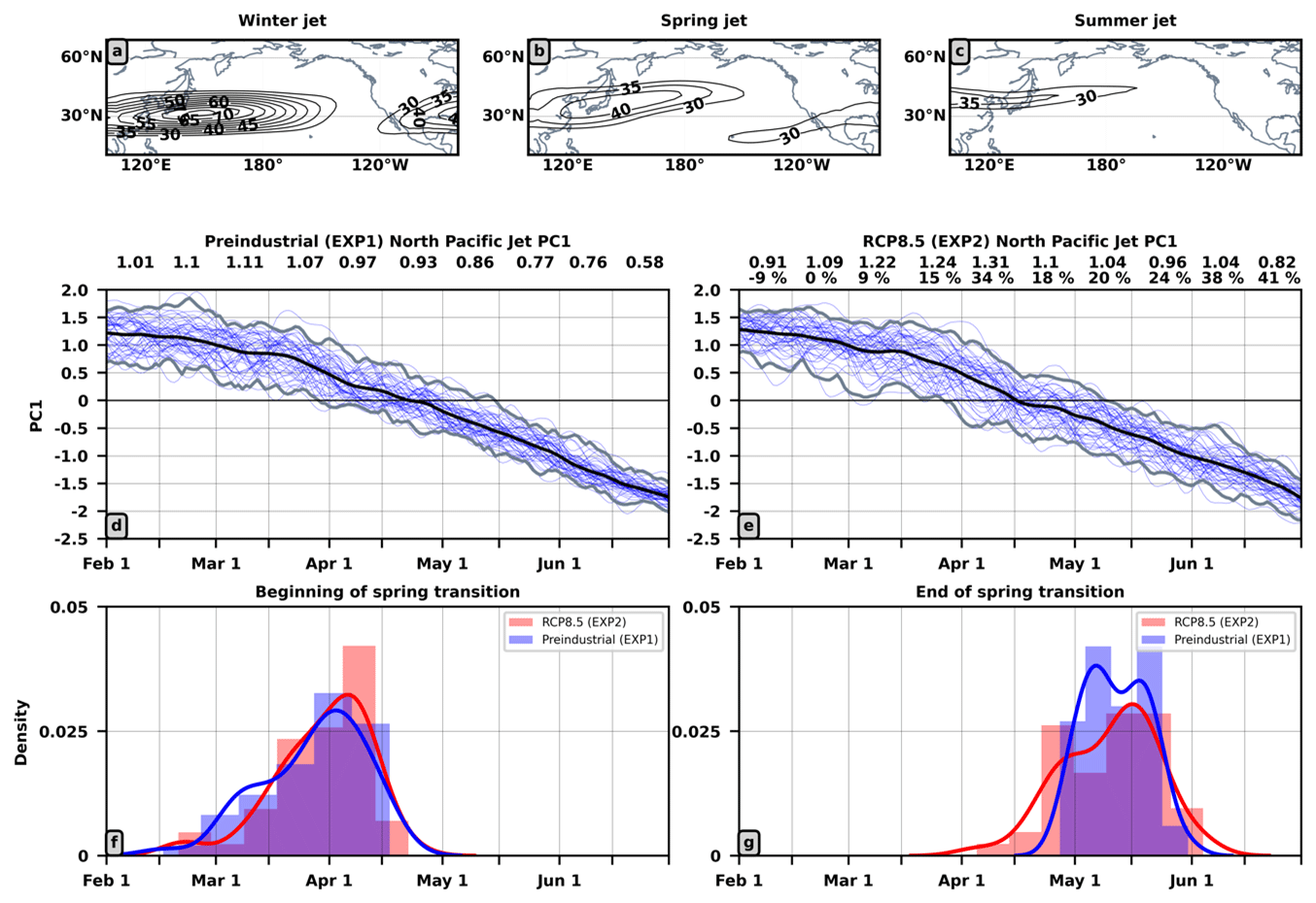
Figure 1 Spring transition of the North Pacific jet in the preindustrial control (EXP1) and the RCP 8.5 experiment (EXP2). Panels (a)–(c) show preindustrial 200 hPa zonal winds subsampled for the jet's winter phase (PC1 > 1σ), spring phase (PC1 < 0.5σ and > −0.5σ), and summer phase (PC1 < −1σ). Panel (d) shows the temporal evolution of PC1 in the preindustrial control (EXP1), with the mean PC1 shown in black, PC1 for each year shown in blue, and the 2.5 % and 97.5 % confidence intervals calculated by bootstrapping with replacement (10 000 times for each day) shown in gray. The average difference between the 2.5 % and 97.5 % confidence intervals for each ∼ 2-week period (referred to as “spread”) are shown above panel (d). Panel (e) is the same as panel (d) but for the RCP8.5 experiment (EXP2). In addition, the percent change between the RCP8.5 and preindustrial spread is also printed above panel (e). Panel (f) and panel (g) are kernel density plots estimating when the spring transition begins (PC1 = 0.5σ) and when the spring transition ends (PC1 = −0.5σ), respectively.

The winter jet is present when PC1 > 1 standard deviation (σ), during which the Pacific jet is strong and narrow (Fig. 1a). The spring jet is present when PC1 < 0.5σ and > −0.5σ, at which point the subtropical jet weakens and shifts north, and the secondary subtropical jet maximum extends between Hawaii and western North America (Fig. 1b). The summer jet is present when PC1 < −1σ (Fig. 1c). The jet weakens substantially and remains shifted poleward, and the secondary jet maximum over North America weakens. The structure of winter, spring, and summer jets (Fig. 1a–c) compares well with that from 1958–2017 Japanese Reanalysis-55 data (cf. Fig. 2, Breeden et al., 2021), as does the timing of the phase changes (Fig. 1d–g; cf. Figs. 1 and 3; Breeden et al., 2021).

The RCP8.5 North Pacific jet exhibits increases in variability compared to the preindustrial control during much of spring and summer (Fig. 1e). Recomputing Fig. 1e using EXP3, which includes RCP8.5 SSTs alone, confirms that the changing jet variability is associated with the SSTs (not shown). Despite these changes in variability, there is no statistically significant change when the spring transition begins (Fig. 1f) or ends (Fig. 1g). The start date for the preindustrial control (EXP1) is 31 March with a σ of ±13 d, and the end date is 11 May ±8 d. For the full RCP8.5 experiment (EXP2), the start date is 1 April with a σ of ±12 d, and the end date is 13 May ±13 d. Consistent with Fig. 1g, the enhanced jet variability due to RCP8.5 conditions manifests as a broader distribution of end dates. With no robust change in the timing of the spring transition, the calendar dates corresponding to the late-winter, spring, and summer jet phases are similar amongst the experiments. Therefore, in all subsequent figures, anomalies are calculated by binning each individual experiment's data according to that experiment's late-winter, spring, and summer days; time-averaging the data within each bin; and then differencing between the jet phase (e.g., late winter) bins from two different experiments (e.g., EXP2 minus EXP1). This approach would not be possible if, for instance, the annually averaged late-winter end date from EXP2 was 10 d after that from the EXP1. Similar results to those shown in Figs. 2–6 can be obtained by comparing like months (e.g., February–March, April–May) from two different experiments (not shown). However, we choose to show our results according to jet phase so that the STT inherently associated with each phase is accounted for.

Note that while no changes in the timing of the spring transition are found in these simulations, spring transition timing is heavily influenced by the El Niño–Southern Oscillation (ENSO; Breeden et al., 2021). Interannual SST fluctuations (which may arise, for instance, due to ENSO) are excluded from our experiments; hence, our results cannot comprehensively establish how RCP8.5 forcing modifies the timing of the spring transition.

2.2 Residual advection, two-way isentropic mixing, production, and loss of O3S

To quantify the contributions of the residual advection, two-way isentropic mixing, and production and loss to the total O3S response, we calculate the terms in the transformed Eulerian mean (TEM) continuity equation for zonal mean tracer transport given by Andrews et al. (1987, Eq. 9.4.13) and discussed by Abalos et al. (2013). Daily data, time-averaged from the 6-hourly fields, are used to calculate each term. These terms are shown in Eq. (1):

$$\begin{array}{}\text{(1)}& {\displaystyle \frac{\partial \stackrel{\mathrm{‾}}{\mathit{\chi }}}{\partial t}}+\stackrel{\mathrm{‾}}{v^{\ast }}{\displaystyle \frac{\partial \stackrel{\mathrm{‾}}{\mathit{\chi }}}{\partial y}}+\stackrel{\mathrm{‾}}{w^{\ast }}{\displaystyle \frac{\partial \stackrel{\mathrm{‾}}{\mathit{\chi }}}{\partial z}}=P-L+e^{-z/H}\mathrm{\nabla }\cdot \mathit{M},\end{array}$$

where overbars denote zonal averages, χ denotes the ozone concentration in parts per billion, P denotes chemical production and L chemical loss, H is the scale height equal to 7 km, y and x are the meridional and zonal Cartesian coordinates, z is log-pressure height, ∇ is the divergence operator, and M is the two-way isentropic mixing vector with meridional and vertical components given by Eqs. (2) and (3):

$$\begin{array}{}\text{(2)}& {\displaystyle }{\mathit{M}}^y=-e^{-\frac{z}{H}}\left(v{}^{\prime }\mathit{\chi }{}^{\prime }-{\displaystyle \frac{\stackrel{\mathrm{‾}}{v{}^{\prime }T{}^{\prime }}}{S}}{\displaystyle \frac{\partial \stackrel{\mathrm{‾}}{\mathit{\chi }}}{\partial z}}\right)\text{(3)}& {\displaystyle }{\mathit{M}}^z=-e^{-\frac{z}{H}}\left(w{}^{\prime }\mathit{\chi }{}^{\prime }+{\displaystyle \frac{\stackrel{\mathrm{‾}}{v{}^{\prime }T{}^{\prime }}}{S}}{\displaystyle \frac{\partial \stackrel{\mathrm{‾}}{\mathit{\chi }}}{\partial y}}\right),\end{array}$$

where primes denote deviations from the zonal average, v and w are the meridional and vertical velocities, S equals $(H\cdot N^{\mathrm{2}})/R$ in which N² is the Brunt–Väisälä frequency, and R is the gas constant equal to 287 m² s⁻² K⁻¹. The residual circulation velocities ($\stackrel{\mathrm{‾}}{v^{\ast }}$, $\stackrel{\mathrm{‾}}{w^{\ast }}$) are given by Eqs. (4) and (5):

$$\begin{array}{}\text{(4)}& {\displaystyle }\stackrel{\mathrm{‾}}{v^{\ast }}=\stackrel{\mathrm{‾}}{v}-{\displaystyle \frac{\mathrm{1}}{{\mathit{\rho }}_{\mathrm{0}}}}{\displaystyle \frac{\partial }{\partial z}}\left({\displaystyle \frac{{\mathit{\rho }}_{\mathrm{0}}\stackrel{\mathrm{‾}}{v{}^{\prime }\mathit{\theta }{}^{\prime }}}{\partial \mathit{\theta }/\partial z}}\right)\text{(5)}& {\displaystyle }\stackrel{\mathrm{‾}}{w^{\ast }}=\stackrel{\mathrm{‾}}{w}+{\displaystyle \frac{\mathrm{1}}{\mathrm{acos}\mathit{\phi }}}{\displaystyle \frac{\partial }{\partial \mathit{\phi }}}\left({\displaystyle \frac{\cos \mathit{\phi }\stackrel{\mathrm{‾}}{v{}^{\prime }\mathit{\theta }{}^{\prime }}}{\partial \mathit{\theta }/\partial z}}\right),\end{array}$$

where ρ₀ is log-pressure density, θ is potential temperature, and a is Earth's radius.

3 Results

3.1 Lower-tropospheric O3S responses

To better understand how climate change may influence the amount of stratospheric ozone making it into the lower free troposphere over western North America, Fig. 2 shows the 700 hPa O3S responses to full RCP8.5 forcing, the change due to SSTs alone, and the change due to GHGs alone for the late-winter, spring, and summer North Pacific jet phases. In the preindustrial control climatology, lower-tropospheric O3S increases from low to high latitudes regardless of season, and mixing ratios are largest over the western North Pacific during the jet's spring phase, mimicking the observed seasonal maximum in deep STT over this region (Fig. 2 black lines; Škerlak et al., 2014; Breeden et al., 2021).

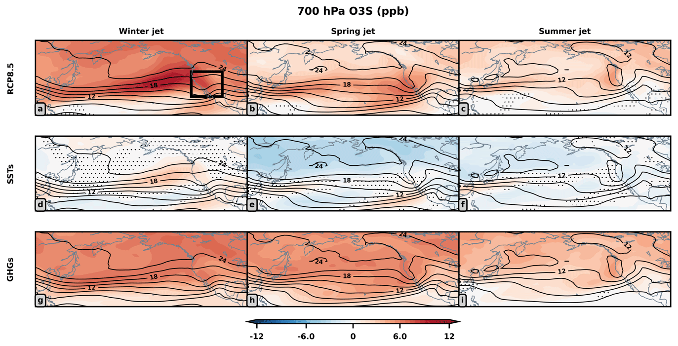
Figure 2 The 700 hPa O3S (ppb) response to RCP8.5 boundary conditions shown in shading. Panels (a)–(c) show the response to RCP8.5 conditions, panels (d)–(f) the response to SSTs alone, and panels (g)–(i) the response to GHGs alone. The 700 hPa O3S preindustrial control seasonal climatologies are overlaid in black. Non-stippled grid points are statistically significant at a 5 % significance threshold using a bootstrapping hypothesis test (Efron and Tibshirani, 1994) in which the two samples being compared are resampled 1000 times at each grid point. The phases of the jet are shown in successive columns. To identify by how much 700 hPa O3S changes over western North America compared to the preindustrial control, spatial averages of the O3S anomalies were taken over the domain boxed in Fig. 2a.

RCP8.5 forcing increases lower-tropospheric O3S over most of the longitudinal domain shown and over much of the hemisphere (not shown) during all three seasons (Fig. 2a–c). The RCP8.5 response is largest in late winter, during which there is up to a 50 % increase in O3S over the North Pacific and a 37 % increase over western North America (25–45^∘ N, 235–260^∘ E; Fig. 2a box). Although the responses are smaller in absolute magnitude during spring and summer compared to winter, they still imply roughly a 10 %–30 % change relative to climatology. Notably in spring, the largest increases are centered over western North America (Fig. 2b).

The SSTs alone (Fig. 2d–f) increase O3S by approximately 15 % over the eastern North Pacific during the jet's late-winter phase (Fig. 2d), explaining a portion of the aforementioned 50 % increase in late winter over this region due to full RCP8.5 forcing (cf. Fig. 2a). Over the low-latitude eastern North Pacific, close to Baja California, Mexico, the SSTs alone promote large increases in O3S during the jet's winter and spring phases relative to preindustrial climate (Fig. 2d–e). Conversely at high latitudes, O3S does not change during the late-winter phase in response to SSTs alone, and it decreases during both the jet's spring and summer phases. In summary, the SSTs alone can explain a portion of the full RCP8.5 response but clearly not the bulk of it.

The response to GHGs alone accounts for the majority of the full RCP8.5 700 hPa O3S response (Fig. 2g–i). Larger O3S increases develop during the jet's late-winter and spring phases compared to summer. Both SSTs alone and GHGs alone increase O3S over the eastern North Pacific and western North America during the jet's late-winter phase but have competing effects on O3S during the jet's spring and summer phases. To better understand the future changes in free tropospheric O3S and the relative roles of SST and GHG changes, the next sections consider in more detail how the North Pacific jet and the lower-stratospheric ozone reservoir respond to climate change.

Figure 3 As in Fig. 2 but for the 200 hPa zonal winds.

3.2 Changes in the upper troposphere and lower stratosphere

RCP8.5 conditions accelerate, narrow, and elongate the late-winter North Pacific jet towards western North America at 200 hPa (Fig. 3a). This change is robust to varying severities of climate change (RCP4.5, Harvey et al., 2020; RCP6.0, Akritidis et al., 2019; and RCP8.5, Matsumura et al., 2021). Contrary to what takes place during the late-winter period, the subtropical jet shifts equatorward during the jet's spring and summer phases (Fig. 3b–c). At lower latitudes, westerly anomalies form over the subtropical eastern Pacific and central America, where there is a climatological minimum in the 200 hPa zonal wind (Fig. 3a–c). This response is present during all three jet phases and strengthens from late winter through summer (Fig. 3a–c).

The full RCP8.5 200 hPa zonal wind response is dominated by the contribution from the SSTs alone (Fig. 3d–f), with the GHGs alone (Fig. 3g–i) playing a comparatively minor role. The strong influence of the SSTs on the wind response arises in part because the SST forcing is associated with almost all of the ∼ 9–11 K warming of the tropical upper troposphere and the amplified Arctic surface warming (Fig. S1) and so dominates the influence on meridional temperature gradients and associated circulation changes that drive heat transport. Another consideration is that the zonal asymmetries in the pattern of SSTs prescribed in the experiments, particularly those over the tropical Pacific resembling El Niño (Fig. S2), may elicit teleconnections (e.g., Pacific North America (PNA) teleconnection pattern) that modify the upper-tropospheric circulation. In general, the impact of the GHGs alone on the 200 hPa winds is small, although the GHGs alone do have a large (compared to climatology) effect on the zonal wind over western North America during the jet's summer phase (Fig. 3i), illustrating that purely chemical changes in the stratosphere are capable of having significant dynamical impacts.

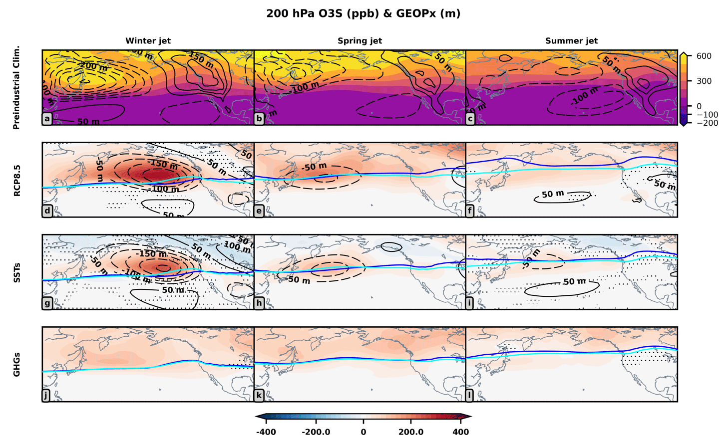
Figure 4 The 200 hPa O3S (shaded, ppb) and stationary wave (“GEOPx”), visualized by geopotential height deviation from its long-term monthly zonal mean (contours, meters), responses to RCP8.5 boundary conditions. Panels (a)–(c) show the preindustrial climatologies of O3S in alternate shading and the climatological stationary wave in contours (d)–(l). Panels (d)–(f) show O3S response to RCP8.5 conditions in shading and stationary wave anomalies as contours, panels (g)–(i) the same but for SSTs alone, and panels (j)–(l) the same but for GHGs alone. Non-stippled grid points are statistically significant O3S anomalies at a 5 % significance threshold using a bootstrapping hypothesis test. The phases of the jet are shown in successive columns. The preindustrial control thermal tropopauses for each season are shown in cyan, and anomalous tropopauses are shown in blue.

Figure 4 shows how RCP8.5 conditions modify 200 hPa O3S, allowing us to see both tropospheric and stratospheric ozone changes; at 200 hPa, the stratosphere is poleward of the anomalous thermal tropopause (blue lines), which can be compared with the preindustrial thermal tropopause (cyan lines) in each season. The 200 hPa O3S equatorward of the tropopause has already been transported into the troposphere and can be lost due to dry deposition, photolysis, and chemical loss or transported back to the stratosphere by reversible mixing processes.

In the preindustrial control (EXP1), O3S maxima and minima are co-located with the troughs and ridges of the climatological stationary wave (Fig. 4a–c). This is particularly clear in late winter, during which O3S mixing ratios exceed 600 ppb over the wave-1-scale trough of the climatological stationary wave, the Aleutian Low (Fig. 4a). O3S mixing ratios are, on the other hand, reduced over the climatological Alaskan ridge. Slightly out of view in Fig. 4a is a climatological wave-2-scale trough that resides over the Baffin Bay and Greenland; an O3S maximum is found over this region as well (Fig. 4a). As suggested by Reed (1950; see also Schoeberl and Kreuger, 1983; Salby and Callaghan, 1993), horizontal advection and vertical motion associated with waves act to concentrate ozone in troughs and reduce it over ridges. The climatological stationary wave influences the 200 hPa composition of O3S in this way.

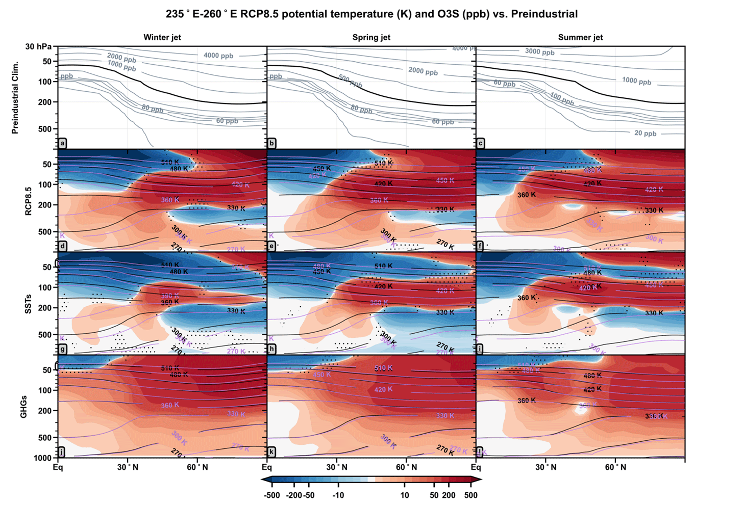
Figure 5 Transects of the O3S anomalies and isentropes averaged between 235 and 260^∘ E (over western North America). Panels (a)–(c) show preindustrial climatologies of O3S; contour intervals are 20, 40, 60, 80, 100, 200, 500 (shown by thick black contour), 1000, 2000, 3000, and 4000 ppb. Panels (d)–(f) show O3S response to RCP8.5 forcing in shading, with preindustrial isentropes shown in black and the anomalous isentropes in magenta; panels (g)–(i) show the same but for SSTs alone and panels (j)–(l) the same but for GHGs alone. Non-stippled grid points are statistically significant O3S responses at a 5 % significance threshold using a bootstrapping hypothesis test. The phases of the jet are shown in successive columns.

Full RCP8.5 conditions increase lower-stratospheric O3S over much of the hemisphere during all seasons (Fig. 4d–f). The largest regional increase is a doubling of O3S over the North Pacific during the jet's late-winter phase (Fig. 4a, d). This regional O3S increase is co-located with the trough of an anomalous tropical–extratropical planetary-scale wave, whose signature is apparent in the zonal wind response (Fig. 3) and the stationary wave response (Fig. 4, black contours). As the amplitude of this wave diminishes during the spring and summer phases, so does the lower-stratospheric O3S maximum (Fig. 4e–f). The RCP8.5 O3S response is mostly contained in the lower-stratospheric (i.e., poleward of the tropopause) trough during the jet's late-winter phase, but in the absence of strong meridional potential vorticity gradients such as the high-latitude polar stratospheric westerlies (Manney et al., 1994; Salby and Callaghan, 2007) or the subtropical jet stream (Bönisch et al., 2009), which serve as transport barriers, the O3S response “smears out” during spring and summer, becoming more evenly distributed around the 200 hPa thermal tropopause (Fig. 4e–f).

The SSTs alone are almost solely responsible for the development of the anomalous planetary wave and are therefore a key reason why there are zonal asymmetries in the lower-stratospheric ozone reservoir (Fig. 4g–i). Similar effects of large-scale planetary wave trains on lower-stratospheric ozone have been noted in relation to ENSO (Zhang et al., 2015; Albers et al., 2022). The SST forcing considered in this study displays SST warming globally but contains some zonal asymmetries, one of them being an El Niño-like eastern tropical Pacific warming (Fig. S2). This zonal asymmetry may explain why the planetary wave response to the SSTs alone during late winter (Fig. 4g) resembles the PNA wave train known to develop with El Niño (albeit the Canadian ridge in Fig. 4g is displaced east relative to the PNA Canadian ridge). Note though that there is large inter-model and inter-generational (CMIP5 vs. CMIP6) spread in how ENSO responds to climate change (Beobide-Arsuga et al., 2021; Cai et al., 2022), suggesting that this planetary wave response could vary amongst climate models should it in fact be related to the El Niño-like warming superimposed on the global SST increase (Fig. S2).

Contrary to the SSTs alone, the GHGs alone have little effect on the planetary-scale eddies and elicit more zonally symmetric O3S responses (Fig. 4j–l). The lower-stratospheric O3S response to the GHGs alone develops largely due to net chemical production of stratospheric ozone, likely associated with the large methane increase in RCP8.5, which enhances O₃ mixing ratios in the extratropical stratosphere (Morgenstern et al., 2018), and changes in transport associated with the BDC's deep branch.

To further clarify how the lower-stratospheric reservoir responds to RCP8.5 conditions, Fig. 5 shows latitude–pressure transects of O3S anomalies and isentropes averaged between 235 and 260^∘ E (over western North America; the same longitudinal bounds used for the box in Fig. 2a). Climatologically, extratropical lower-stratospheric O3S mixing ratios are larger during winter and spring (Fig. 5b), following from transport by the BDC's deep branch (Ray et al., 1999; Hegglin and Shepherd, 2007; Bönisch et al., 2009; Butchart, 2014; Konopka et al., 2015; Ploeger and Birner, 2016; Albers et al., 2018). During summer in climatology, enhanced isentropic mixing between the tropical and extratropical lowermost stratosphere (Hegglin and Shepherd, 2007; Abalos et al., 2013) and rising tropopause heights (Schoeberl et al., 2004) act to flush ozone out of the lowermost stratosphere.

During every jet phase, RCP8.5 conditions reduce O3S in the low-latitude stratosphere while promoting accumulation of O3S at high latitudes (Fig. 5d–f). Some of this O3S accumulating in the extratropical lower stratosphere may enter the troposphere along the subtropical upper-tropospheric and lower-stratospheric isentropes (e.g., 360 K). Both the GHGs alone and SSTs alone play a role in making this happen. The upper-tropospheric warming induced by the SSTs alone depresses the isentropes (e.g., 360 K) to lower altitudes, enhancing the access of the troposphere to lower-stratospheric air (Fig. 5g–i), where wave breaking is able to transport the ozone into the subtropical and tropical upper troposphere (e.g., Waugh and Polvani, 2000; Albers et al., 2016, and references therein). The GHGs alone on the other hand mainly contribute by more broadly enhancing the extratropical lower-stratospheric O3S concentrations (Fig. 5j–l).

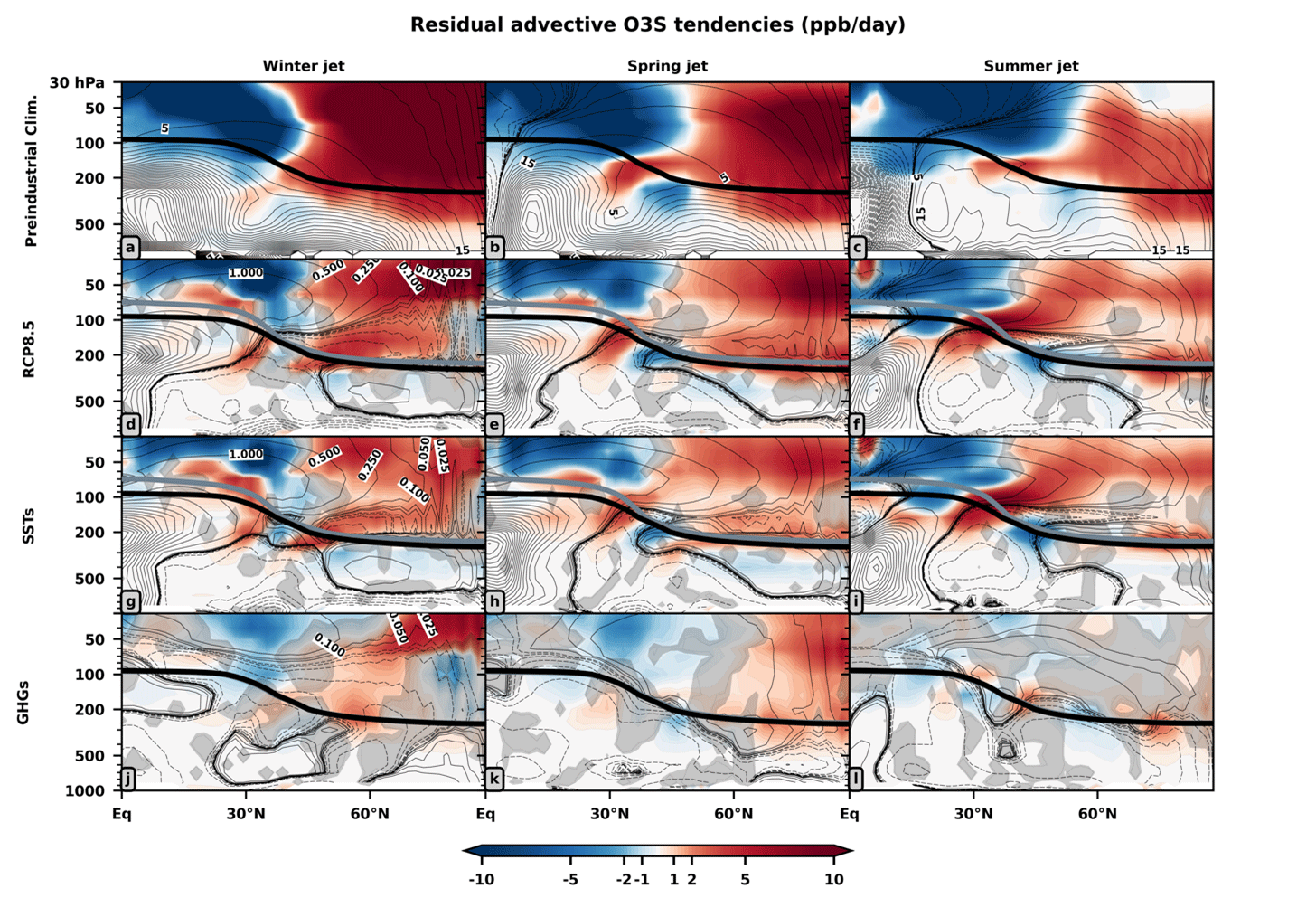
Figure 6 Residual advective O3S tendencies (shading) and residual mass streamfunction (contours). Panels (a)–(c) show preindustrial residual advective O3S tendencies in shading, with the climatological residual mass streamfunction overlaid in black contours. The color scale is the same for the climatology and anomalies. The contour intervals for the residual mass streamfunction in all panels are 0.025, 0.05, 0.1, 0.25, 0.5, 1, 5, 10, 15, 20, 25, etc. (10⁹ kg s⁻¹). Panels (d)–(f) show the O3S tendency and streamfunction anomalies to RCP8.5; panels (g)–(i) show the same but for SSTs alone and panels (j)–(l) the same but for GHGs alone. Non-gray shaded grid points show statistically significant O3S tendency anomalies at a 5 % significance threshold using a bootstrapping hypothesis test. The phases of the jet are shown in successive columns. For each phase of the jet, the preindustrial control thermal tropopause is black, and the anomalous tropopause is gray. Note that an anomalous tropopause is hardly visible in response to GHGs alone, as the SSTs alone are the forcing that modifies the tropopause.

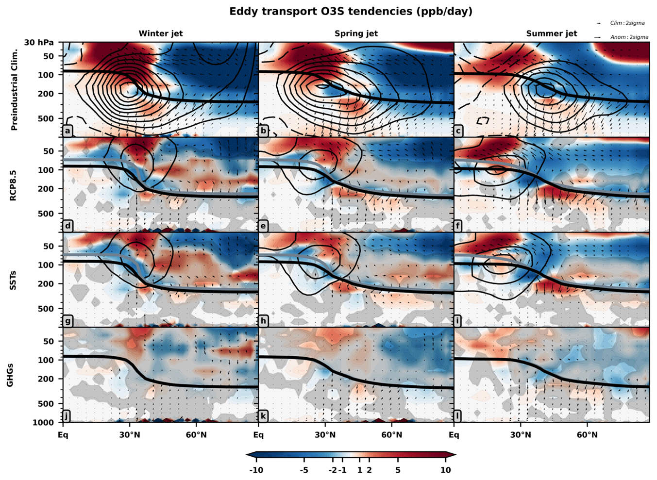
Figure 7 Two-way isentropic mixing O3S tendencies (shading) and zonal mean zonal wind (contours). Panels (a)–(c) show preindustrial O3S tendencies in shading, with the climatological zonal wind overlaid in black (±5 m s⁻¹), and the components of the two-way isentropic mixing (−M_y, −M_z) shown as vectors. The color scale is the same for the climatology and anomalies. Panels (d)–(f) show the O3S tendency and zonal wind anomalies to RCP8.5; panels (g)–(i) show the same but for SSTs alone and panels (j)–(l) the same but for GHGs alone. Non-gray shaded grid points show statistically significant O3S anomalies at a 5 % significance threshold using a bootstrapping hypothesis test. The phases of the jet are shown in successive columns. For each phase of the jet, the preindustrial control thermal tropopause is black, and the anomalous tropopause is gray.

O3S is reduced near the extratropical tropopause in all seasons in response to RCP8.5 forcing (Fig. 5d–f). This is associated with the increased height of the tropopause (Abalos et al., 2017) resulting from the SSTs alone. Due to steep vertical gradients in tracers near the tropopause (e.g., Pan et al., 2004), taking the difference between an experiment with a lifted tropopause (EXP2 or EXP3) and an experiment without this feature (preindustrial control, EXP1) amounts to taking the difference between relatively O3S-depleted tropospheric air and O3S-rich stratospheric air; hence, the negative O3S anomalies develop near the tropopause (Fig. 5d–i). This negative O3S response can largely be removed by remapping the vertical axis of each data field used to make, for instance, Fig. 5d–f (zonally averaged RCP8.5 (EXP2) O3S and preindustrial (EXP1) O3S) to tropopause-relative coordinates (meters above or below the thermal tropopause), then taking the difference between these two modified data fields and remapping this set of anomalies (axes: tropopause-relative × latitude) to a log-pressure coordinate system (axes: pressure × latitude) (Abalos et al., 2017). Using annual cycles of thermal tropopause and O3S data, which should help to smooth out the large hourly/daily fluctuations in these fields near the tropopause, the aforementioned procedure was applied to a zonally averaged transect over the North Pacific (Fig. S3) and applied at all grid points at 200 hPa (Fig. S4) and 300 hPa (Fig. S5). While this tropopause-relative analysis does remove the majority of the negative O3S response associated with the tropopause lift, the strong O3S zonal asymmetries associated with the planetary wave response to the SSTs alone persist, namely the negative O3S response corresponding to the planetary wave's ridge near Alaska (cf. Figs. 4k, S5e). This analysis corroborates that the higher tropopause in RCP8.5 is largely responsible for the presence of the negative O3S response in the extratropical upper troposphere and lower stratosphere, however, not entirely, as we find that a portion of this negative O3S is associated with the anomalous planetary wave's zonally asymmetric effects on the upper-tropospheric and lower-stratospheric O3S distribution.

3.3 Zonally symmetric changes

The seasonal variability of both tropical (Abalos et al., 2013) and extratropical (Albers et al., 2018) lower-stratospheric ozone tendencies is heavily influenced by upwelling and downwelling associated with BDC's residual mean meridional circulation component. This circulation is made up of a shallow and a deep branch. Transport associated with the shallow branch proceeds more horizontally, and the air masses enter the stratosphere closer to the subtropics, whereas transport associated with the deep branch is more vertical, and the air masses enter the stratosphere through the deep tropics and descend at high latitudes (Birner and Bönisch, 2011). To quantify the influence of RCP8.5 forcing on these physical processes, Fig. 6 shows the residual mass streamfunction response to RCP8.5 forcing in black contours and in shading the local changes in O3S tendencies as a result of transport by the residual mean meridional circulation terms in the TEM continuity equation ($\stackrel{\mathrm{‾}}{v^{\ast }}\frac{\partial \stackrel{\mathrm{‾}}{\mathit{\chi }}}{\partial y}+\stackrel{\mathrm{‾}}{w^{\ast }}\frac{\partial \stackrel{\mathrm{‾}}{\mathit{\chi }}}{\partial z}$). As in reanalysis (cf. Rosenlof, 1995), in the preindustrial control, the tropical upward mass flux peaks in amplitude during boreal winter when the residual mass streamfunction is strongest (Fig. 6a). As the zonal momentum budget changes in each hemisphere during spring and summer, the tropical upward mass flux shifts into the Northern Hemisphere, and the residual mass streamfunction weakens and shifts downward towards the troposphere (Fig. 6b, c). The negative O3S tendencies in the tropical lower stratosphere track the latitudinal shifting of the tropical upward mass flux over time. The positive O3S tendencies in the extratropical lower stratosphere associated with poleward transport of stratospheric ozone from its tropical source region peak in amplitude during winter when the BDC's deep branch is strongest and weaken thereafter.

RCP8.5 forcing strengthens the shallow branch of the BDC during all three seasons, reducing tropical stratospheric O3S tendencies (Fig. 6d–f). The SSTs alone (Fig. 6g–i) are primarily responsible for the acceleration of the residual mass streamfunction in the subtropical lower stratosphere (50 hPa/30^∘ N) when compared against the GHGs alone (Fig. 6j–l), consistent with Oberländer et al. (2013) and Chrysanthou et al., (2020). The upper component of the Hadley circulation near 150 hPa and 15^∘ N accelerates, as previously reported by Abalos et al. (2020). All models that they studied included this response. This feature acts cooperatively with the reinforced BDC shallow branch to increase O3S transport through the subtropical tropopause into the upper troposphere (200 hPa and 30^∘ N), with the largest increase occurring during summer in response to the SSTs alone (Fig. 6i). The GHGs alone accelerate the deep branch well above 30 hPa during winter (Fig. 6j); the deep branch's high-latitude downwelling increases lower-stratospheric O3S during spring (Fig. 6k) and then disappears by summer (Fig. 6i).

Another aspect of the BDC is two-way isentropic mixing, which climatologically increases subtropical O3S tendencies above and south of the subtropical jet, while reducing extratropical O3S tendencies throughout the stratosphere (Fig. 7a–c). In the tropical lower stratosphere (∼ 80 hPa), tendencies peak during summer in present-day analyses (Abalos et al., 2013) and in the preindustrial control climatology (Fig. 7c). RCP8.5 forcing generally reinforces the climatological two-way isentropic mixing in the stratosphere during each season, increasing subtropical tendencies and reducing extratropical tendencies (Fig. 7d–f). Additionally, enhanced cross-tropopause mixing by eddies increases upper-tropospheric O3S tendencies from 30–60^∘ N, with stronger signals during summer than winter. These anomalies are primarily associated with the SSTs alone (Fig. 7g–i). Hardly any part of the two-way isentropic mixing responses to GHGs alone are statistically significant (Fig. 7j–l).

4 Conclusions

We use three interactive-chemistry WACCM experiments to analyze how stratosphere-to-troposphere transport of ozone over western North America during late winter, spring, and summer responds to worst-case scenario RCP8.5 climate change at the end of the century. Lower-tropospheric O3S concentrations increase up to 37 % during late winter over western North America in response to RCP8.5 forcing, with progressively weaker increases during spring and summer. Between the GHGs alone and SSTs alone, the GHGs alone are found to be primarily responsible for increase in lower-tropospheric O3S over western North America and across the Northern Hemisphere.

Because lower-stratospheric ozone mixing ratios are positively correlated with the amount of ozone contained in intrusions that transport mass into the troposphere (Ordóñez et al., 2007; Hess and Zbinden, 2013; Neu et al., 2014; Albers et al., 2016, 2018), we document the processes modifying future lower-stratospheric ozone. The portion of the full RCP8.5 response driven by the GHGs alone (no changes to the SSTs) promotes higher ozone mixing ratios throughout the extratropical lower stratosphere. It is unlikely that these increases are associated with dynamical changes due to GHGs alone. In agreement with Oberländer et al. (2013) and Chrysanthou et al. (2020), we find that the GHGs alone modify residual advective transport, promoting some increases in extratropical lower-stratospheric ozone. However, this response, in combination with the weak eddy transport response to the GHGs alone, cannot wholly explain the changes in extratropical lower-stratospheric O3S that occur during winter, spring, and summer due to GHGs; thus, we conclude that production of ozone must be an important component of the response to GHGs. Note that different GHGs have unique chemical influences on ozone (e.g., Fleming et al., 2011), which we do not attempt to separate in this study (see Morgenstern et al., 2018). We hypothesize that the higher tropospheric O3S driven by GHGs alone is associated with enhanced production of ozone throughout the extratropical lower stratosphere, likely due to 4.6 times higher methane concentrations in the RCP8.5 experiment compared to the preindustrial control (Portmann and Solomon, 2007; Revell et al., 2012; Morgenstern et al., 2018; Winterstein et al., 2019). The ozone increases evidently outweigh any ozone reductions forced by the 1.5 times and 3 times increases in N₂O and Cl_y, respectively, culminating in a net ozone increase throughout the extratropical lower stratosphere (Fig. 5j–k).

The SSTs alone promote scattered regional increases and decreases in lower-tropospheric O3S. Over the North Pacific, the lower-tropospheric O3S increases are co-located with the low-pressure center of the largest anomalous trough of a tropics–extratropics planetary-scale wave that forms over the North Pacific, similar to the PNA wave train, in response to the SSTs alone. When the amplitude of this wave is largest (during late winter), O3S increases by nearly 400 ppb within the wave's largest trough at 200 hPa, a doubling of O3S relative to the preindustrial control climatology. A large part of this trough is located in the lower stratosphere at 200 hPa, illustrating that planetary waves can introduce high-amplitude zonal asymmetries into the lower-stratospheric ozone reservoir that then coincide with regionally enhanced STT. In agreement with Reed (1950), we attribute the co-location between lower-stratospheric troughs (ridges) and enhanced (reduced) ozone to horizontal advection and vertical motion induced by the North Pacific planetary-scale wave. Although their studies focus on ENSO, Zhang et al. (2015) and Albers et al. (2022) each provide more detailed observational and model-based evidence in favor of this physical mechanism.

One interesting result is that the quasi-zonally symmetric increase in lower extratropical stratospheric ozone due to the GHGs alone (Fig. 4j–k) mirrors the quasi-zonally symmetric increase in lower-tropospheric O3S below it (Fig. 2j–k). Similarly, the highly regional changes in lower extratropical stratospheric ozone forced by the SSTs alone (Fig. 4g–i) are co-located to, but above, the regional changes in lower-tropospheric O3S forced by the SSTs alone (Fig. 2g–i). Taken together, these results suggest that the spatial distribution of ozone in the lower-stratospheric reservoir informs the spatial distribution of lower-tropospheric O3S responses; similar conclusions may be drawn from Albers et al. (2022; cf. their Figs. 4 and 8).

The SSTs alone are found to increase the year-to-year variability of the North Pacific jet's seasonal evolution, particularly during spring and summer, broadening the distribution of days on which the spring transition may end, which in theory could coincide with more erratic year-to-year fluctuations in STT of ozone in the future. Despite this, we find no statistically significant change in the timing of the spring transition in response to full RCP8.5 forcing. Since the experiments use fixed repeating annual cycles of sea surface temperature and therefore exclude interannual SST fluctuations, which are known to modify the seasonal variability of the North Pacific jet (Langford, 1999; Zhang et al., 2015; Breeden et al., 2021; Albers et al., 2022), our results cannot be used to comprehensively establish whether or not the seasonal variability of the North Pacific jet, particularly its spring transition, will change in response to climate change. Our results do, however, illustrate that changes in SSTs have a strong effect on the North Pacific jet, and in general, the SSTs alone account for the majority of changes to the large-scale atmospheric circulation in the full RCP8.5 forcing. For example, the SSTs alone drive the acceleration and elongation of the late-winter North Pacific jet, the equatorward shift of the spring and summer North Pacific jet, the acceleration of the BDC's shallow branch, some of the deep branch acceleration, and most of the two-way isentropic mixing responses. Considering that the SSTs alone account for many of the changes to the large atmospheric circulation, an avenue for future research is to analyze inter-model spread in the future residual mean circulation response (Oman et al., 2010; Butchart, 2014; Abalos et al., 2021) and the two-way isentropic mixing response (Eichinger et al., 2019; Abalos et al., 2020) as a function of inter-model spread in future SSTs.

Given that the response to GHGs alone accounts for the majority of the full RCP8.5 lower-tropospheric O3S response over western North America, it is interesting to consider how a different climate change scenario may impact our tropospheric O3S responses. Future STT exhibits large inter-scenario spread (Young et al., 2013). Considering that RCP4.5, RCP6.0, and RCP8.5 use equivalent Cl_y emissions (Meinshausen et al., 2011), it seems more likely that the results herein would change due to the different concentrations of CH₄, N₂O, and CO₂ prescribed under the other scenarios, as opposed to the Cl_y. In particular, lower concentrations of CH₄ would likely coincide with a smaller net increase in extratropical lower-stratospheric ozone (e.g., Revell et al., 2012) and therefore reduced STT of ozone over western North America. Indeed, tropospheric column ozone decreases by the end of the century under RCP2.6 and RCP4.5 but increases due to RCP8.5 conditions (Archibald et al., 2020), although to be clear, many factors (e.g., ozone precursors, Young et al., 2013) and not just STT will influence future tropospheric ozone. A different climate change scenario would also produce a different dynamical response to climate change; for instance, the strength of the BDC shallow branch response to climate change scales with the change in future tropical surface temperature warming (Abalos et al., 2021) and the change in future global SSTs (Chrysanthou et al., 2020). This suggests that a different climate change scenario would beget a different planetary wave response over the North Pacific and, hence, different regional STT responses. For climate change scenarios with weaker radiative forcing change and presumably less production of extratropical lower-stratospheric ozone, the dynamical response to the SSTs alone under these scenarios may play a more important role in influencing STT of ozone than we find herein with the RCP8.5 scenario.