Exploring the drivers of tropospheric hydroxyl radical trends in the Geophysical Fluid Dynamics Laboratory AM4.1 atmospheric chemistry–climate model

We explore the sensitivity of modeled tropospheric hydroxyl (OH) concentration trends to meteorology and near-term climate forcers (NTCFs), namely methane (CH₄) nitrogen oxides $({\mathrm{NO}}_x={\mathrm{NO}}_{\mathrm{2}}+\mathrm{NO})$ carbon monoxide (CO), non-methane volatile organic compounds (NMVOCs) and ozone-depleting substances (ODSs), using the Geophysical Fluid Dynamics Laboratory (GFDL)'s atmospheric chemistry–climate model, the Atmospheric Model version 4.1 (AM4.1), driven by emissions inventories developed for the Sixth Coupled Model Intercomparison Project (CMIP6) and forced by observed sea surface temperatures and sea ice prepared in support of the CMIP6 Atmospheric Model Intercomparison Project (AMIP) simulations. We find that the modeled tropospheric air-mass-weighted mean [OH] has increased by ∼5 % globally from 1980 to 2014. We find that NO_x emissions and CH₄ concentrations dominate the modeled global trend, while CO emissions and meteorology were also important in driving regional trends. Modeled tropospheric NO₂ column trends are largely consistent with those retrieved from the Ozone Monitoring Instrument (OMI) satellite, but simulated CO column trends generally overestimate those retrieved from the Measurements of Pollution in The Troposphere (MOPITT) satellite, possibly reflecting biases in input anthropogenic emission inventories, especially over China and South Asia.

1 Introduction

The hydroxyl radical (OH), as the primary daytime oxidant in the troposphere (Levy, 1971), plays an important role in atmospheric chemistry. OH influences air quality and climate, as reaction with OH is a major sink of various trace species including tropospheric ozone precursors such as methane (CH₄), carbon monoxide (CO), and nitrogen oxides $({\mathrm{NO}}_x=\mathrm{NO}+{\mathrm{NO}}_{\mathrm{2}})$; ozone-depleting substances (ODSs) such as halocarbons; and non-methane volatile organic compounds (NMVOCs) (e.g., Holmes et al., 2013; Turner et al., 2019). Precise knowledge of the OH budget, its variations and trends, and its response to various drivers is needed to determine source and sink budgets for these important trace species and is therefore crucial to our understanding of the various aforementioned effects on the Earth system (e.g., Lawrence et al., 2001; Naik et al., 2013; Murray et al., 2014; Zhao et al., 2019; Nicely et al., 2020; Patra et al., 2021). In particular, there are still gaps in our understanding of the drivers of the observed atmospheric methane concentration growth rate in recent years (Saunois et al., 2020; Nisbet et al., 2021), further highlighting the importance of better understanding [OH] trends and variability. Recent observation-based studies suggest either a decline or stable OH concentrations over the past 4 decades (e.g., Rigby et al., 2017; Turner et al., 2017; Zhao et al., 2019), while global chemistry–climate models simulate increases over the same period (e.g., Stevenson et al., 2020; Zhao et al., 2020). In this study, we employ the state-of-the-science Geophysical Fluid Dynamics Laboratory (GFDL) chemistry–climate model (CCM), AM4.1, to systematically explore the drivers of changes in [OH] between 1980 and 2014 to shed light on its role in driving recent methane increases.

Changes in [OH] can be traced back to changes in the budget terms. The time tendency of [OH] is determined by the balance between chemical production (P) and loss (L) terms, since the chemical processes for OH tend to occur at much faster timescales compared to other potential terms in the budget equation such as advection and transport (Lelieveld et al., 2016). The governing time tendency equation therefore is given by

$$\begin{array}{}\text{(1)}& {\displaystyle \frac{\mathrm{d}\left[\mathrm{OH}\right]}{\mathrm{d}t}}=P-L.\end{array}$$

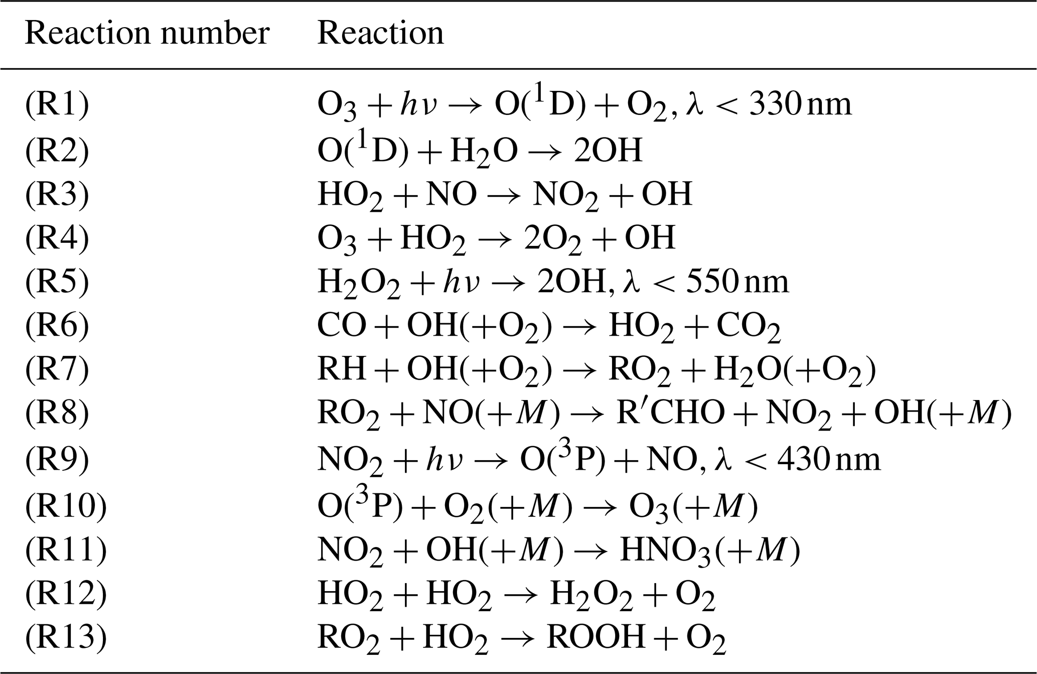
Table 1 summarizes the tropospheric OH chemistry that is described here. Primary production of tropospheric OH occurs via the photodissociation of tropospheric ozone (O₃) by ultraviolet (UV) radiation of wavelength less than 310 nm (Reaction R1) to produce excited singlet oxygen atoms (O(¹D)) (Brasseur and Solomon, 2005), which then react with water vapor (Reaction R2). OH can also be generated by secondary production mechanisms that recycle OH from hydroperoxy radicals (HO₂) (Reactions R3–R5). In high-NO_x regions, such as polluted urban environments, HO₂ can be recycled back to OH via reaction with NO without consuming O₃ (Reaction R3) and is the dominant production term. This NO_x-driven secondary production of OH, otherwise known as the NO_x recycling mechanism of OH, is similar in magnitude to the primary formation of OH on a global basis, being about ∼30 % each (Lelieveld et al., 2016). In unpolluted regions, other secondary production mechanisms, collectively called the O_x recycling mechanism, are dominant. One involves the consumption of ozone in unpolluted regions (Reaction R4) (as opposed to the production of ozone in polluted conditions), and the other involves the photolysis of H₂O₂ (Reaction R5). Oxidation of CO is the largest OH loss reaction (Reaction R6) with important losses via oxidation of methane and non-methane volatile organic compounds (NMVOCs) (Reaction R7). Organic peroxy radicals can also undergo an OH-recycling reaction with NO to form NO₂ (Reaction R8). The fate of the resultant organic carbon product, R^′CHO, can be to either further generate OH or HO₂ radicals if it undergoes photolysis or to undergo further oxidation by OH. The NO₂ produced via Reactions (R3) and (R8) can then be photolyzed to form ozone (Reactions R9–R10), which then leads to further primary production of OH via Reactions (R1) and (R2) (Hameed et al., 1979). In a strongly polluted atmosphere, NO₂ can locally become a large HO_x $({\mathrm{HO}}_x=\mathrm{OH}+{\mathrm{HO}}_{\mathrm{2}})$ sink, causing net OH loss through the formation of nitric acid (HNO₃) (Reaction R11), which can be washed out via wet deposition (Crutzen and Lawrence, 2000). Meanwhile, in clean, non-polluted conditions, the reaction chains involving the HO₂ and RO₂ radicals can be terminated via loss Reactions (R12) and (R13). The self-reaction of HO₂ (Reaction R12) represents an OH sink, as the hydrogen peroxide (H₂O₂) product can be washed out via wet deposition and is the dominant HO_x sink since most of the troposphere experiences low-NO_x conditions (Jaeglé et al., 2001).

Table 1 Important reactions describing tropospheric OH chemistry.

Overall, the atmospheric composition directly impacts the OH budget, most notably via tropospheric ozone, humidity, NO_x, CO, methane and NMVOCs, with the former three usually acting to increase [OH] and the latter three acting to decrease [OH], but there are also meteorological factors that influence the budget via influencing the tropospheric chemistry of OH as well. Temperature plays an important role in controlling rate reaction rates, tropospheric water vapor abundance and also natural emissions of biogenic VOCs (Spivakovsky et al., 2000). Also, as many important reactions are photolysis reactions, such as the primary production of OH via Reaction (R1) which requires UV radiation of wavelengths (λ<330 nm), the overhead ozone column, which controls the amount of UV radiation penetrating into the troposphere, aerosol direct and indirect effects, and cloud cover play an important role as well (Levy, 1971). These point to the possible anthropogenic impacts on the OH budget that can impact these various factors directly or indirectly.

Because OH is highly reactive and therefore has a short lifetime of ∼1 s, this makes it difficult to achieve global observational coverage over time of directly observed [OH]. As a result, various observational proxies have been used to indirectly estimate the spatial distribution, global mean, and the temporal variations and trends of [OH]. A widely used proxy is methyl chloroform (CH₃CCl₃, MCF) (e.g., Montzka et al., 2011; Rigby et al., 2017; Turner et al., 2017; Naus et al., 2019; Patra et al., 2021), for which there is a relatively long temporal observational record, for example the ∼4 decades' worth of data from the Advanced Global Atmospheric Gases Experiment (AGAGE) and National Oceanic and Atmospheric Administration (NOAA) networks. Using a multi-box model inversion method, Rigby et al. (2017) and Turner et al. (2017) found an increasing global mean [OH] trend from the 1990s up to the mid-2000s but found a decreasing [OH] trend thereafter; however, in these studies, it was highlighted that the inferred [OH] trends were only weakly constrained, and when Naus et al. (2019) corrected for biases in the multi-box model inversion method, they found an overall increasing trend over the last 2 decades. To avoid some of these biases such as those arising from the spatial averaging required in box model methods, 3D chemistry transport models (CTMs) have also been used to infer [OH] from MCF observations such as in Patra et al. (2021) and Naus et al. (2021), who found no significant trend in [OH]. Non-MCF methods have also been used to explore [OH] trends since 1980: for example, Nicely et al. (2018) used observational constraints of various [OH] drivers to empirically reconstruct [OH] and found no significant trend as well. Overall, global mean [OH] derived from most atmospheric inversions or empirical reconstructions seems to not have a significant trend over the 1980–2014 period. Models such as CTMs, CCMs, and Earth system models (ESMs) can also be used to calculate [OH], and these models have shown an increase in global mean [OH] since 1980 to present day, in contrast to the [OH] trends derived from observational constraints (Naik et al., 2013; Zhao et al., 2019; Nicely et al., 2020; Stevenson et al., 2020; Zhao et al., 2020). Most of these studies found that changes to Near-term Climate Forcers (NTCFs) played a key role in driving the modeled [OH] increase. In particular, Stevenson et al. (2020) found an ∼10 % increase with respect to the 1998–2007 mean from 1980 to 2014 from three Earth system models (ESMs) participating in the Aerosols and Chemistry Model Intercomparison Project (AerChemMIP) as part of the Sixth Coupled Model Intercomparison Project (CMIP6). They attribute this simulated increase to changes in anthropogenic NTCFs, mainly increases in anthropogenic nitrogen oxides combined with declining CO emissions since 1990 with smaller contributions from changes in halocarbon and aerosol-related emissions. Naik et al. (2013) and Nicely et al. (2020) also additionally highlight the role of stratospheric ozone loss due to factors such as emissions of ozone-depleting substances (ODSs) and increasing specific humidity in driving the increasing [OH] trend.

As discussed above, there are a plethora of emissions-related chemical and physical drivers that affect [OH], and many of these are also driven by climate variability (Alexander and Mickley, 2015). As such, [OH] tends to exhibit interannual variability (IAV), and various modeling studies have explored the drivers of [OH] IAV. For example, large-scale climate variability through the El Niño–Southern Oscillation (ENSO) has been shown to play an important role in driving [OH] IAV through ENSO effects on variability in temperature and humidity (Zhao et al., 2020), biomass burning emissions such as CO (an OH sink) and NO_x (tends to enhance OH) (Holmes et al., 2013; Zhao et al., 2020), O₃ and j(O¹D) in the lower troposphere (Anderson et al., 2021), and lightning NO_x emissions (Turner et al., 2018). In particular, the role of lightning NO_x in driving [OH] IAV in the GFDL AM4.1 over the period 1980–2016 was also highlighted by He et al. (2021) and Murray et al. (2013), who found that lightning NO_x emissions were the key factor driving IAV, especially over the period 1998–2006, through its role in affecting both secondary OH production via the NO_x recycling mechanism and primary production via its role as a tropospheric ozone precursor. However, the drivers of OH variability also show large model diversity. For example, lightning NO_x can be parameterized differently in different models (Zhao et al., 2020; Wild et al., 2020), and so its response to climate variability like ENSO can vary from model to model.

In summary, in the period 1980–2014, global CCMs seem to have converged on an overall increasing [OH] trend driven by complementary changes in emissions and meteorology (Szopa et al., 2021). Here we build on previous studies to explore the contribution of individual component drivers to attribute trends and variability in [OH]. We apply the GFDL-AM4.1 CCM to systematically explore the roles of meteorology and individual chemical drivers in changing [OH], with the goal of identifying the primary drivers of increasing [OH] trends over 1980–2014 simulated by global models. Additionally, we analyze the model simulations to shed light on the primary drivers of [OH] IAV.

2 Methods

2.1 GFDL AM4.1 model setup

We use the GFDL Atmospheric Model 4.1 (AM4.1), which is the atmosphere-only configuration of the GFDL Earth System Model ESM4.1. Further details of the AM4.1 setup are described by Horowitz et al. (2020), and a summary of the features relevant to [OH] are provided here. The AM4.1 has a spatial resolution of ∼100 km on a cubed-sphere grid and resolves 49 vertical levels up to ∼80 km. It uses an updated chemical mechanism (Horowitz et al., 2020) with gas-phase and heterogeneous chemistry updates following Mao et al. (2013a, b). The key feature of this model configuration is that it has online oxidants; i.e., it includes chemical and climate feedbacks on oxidant concentrations. Photolysis rate constants are calculated interactively via the photolysis mechanism Fast-JX version 7.1 (Wild et al., 2000; Bian and Prather, 2002). All model simulations are forced with interannually varying sea surface temperatures and sea ice from Taylor et al. (2000), prepared in support of the Atmospheric Model Intercomparison Project (AMIP) simulations as part of phase 6 of the Coupled Model Intercomparison Project (CMIP6).

We used historical emissions datasets for ozone and aerosol precursors developed in support of CMIP6: the Community Emissions Database (CEDS) for anthropogenic emissions (v2017-05-18; Hoesly et al., 2018) and historical biomass burning emissions for CMIP6 (BB4CMIP) for biomass burning emissions (van Marle et al., 2017). In addition, natural sources of NMVOCs, NO_x, and CO were taken from Precursors of Ozone and their Effects in the Troposphere inventory (POET, Granier et al., 2005) following Naik et al. (2013), except for isoprene and monoterpene emissions which are calculated online as described in Horowitz et al. (2020) and Rasmussen et al. (2012). As described in Horowitz et al. (2020), lightning NO_x emissions are calculated interactively as a function of subgrid convection, as diagnosed by the double plume convection scheme described by Zhao et al. (2018). The lightning NO_x source is calculated as a function of convective cloud-top height, following the parameterization of Price et al. (1997), and is injected with the vertical distribution of Pickering et al. (1998). Well-mixed greenhouse gas concentrations are specified following Meinshausen et al. (2017). In particular, atmospheric concentrations of ODSs, including CFC-11, CFC-12, CFC-113 and HCFC-22, and CH₄ concentrations are specified at the surface as a global mean lower boundary condition, with concentrations beyond the surface subsequently determined by various chemical and dynamical processes. A summary of historical CO emissions, CH₄ concentrations, and NO_x emissions is shown in Fig. 1.

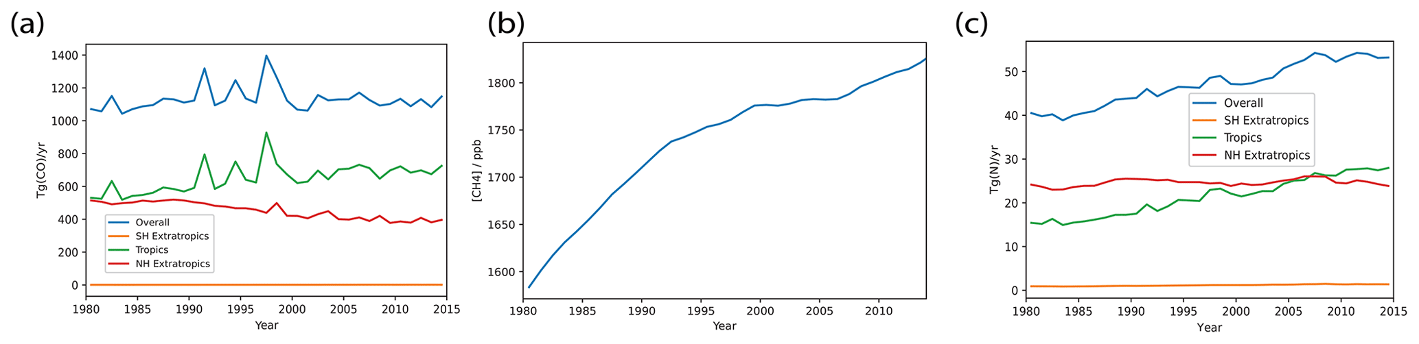
Figure 1 Historical time series of (a) regional CO emissions, (b) CH₄ surface concentrations and (c) regional NO_x emissions used for this study. The Southern Hemisphere (SH) extratropics are defined as 90–30^∘ S, the tropics are defined as 30^∘ S–30^∘ N, and the Northern Hemisphere (NH) extratropics are defined as 30–90^∘ N. Globally, CH₄ concentrations have increased by ∼16 %. Non-lightning NO_x emissions have also increased by ∼30 % globally over this period, with this increase driven by the tropics. CO emissions see IAV but little trend globally over this period, but they do see a decreasing trend in the NH extratropics offset by an increasing trend in the tropics.

2.2 Model runs

We conducted model integrations from 1980–2014 using an initialization state from an GFDL AM4.1 historical run. In addition to a “Base” run that includes the time-varying historical emissions of the various species as per Horowitz et al. (2020), we conducted “all-but-one” runs where we investigate the effects of various emitted species that could affect OH concentrations, namely NO_x, CH₄, CO, NMVOC, and ozone-depleting substances (ODSs). These runs are configured so as to systematically fix the emissions of a particular species to 1980 values in order to isolate the effects of each individual species by comparing them with the Base run. Additionally, we include a run where all the above species are set to 1980 values (“Met”), which allows us to diagnose the effects of meteorology. Note that as lightning NO_x emissions and biogenic terpene and isoprene emissions are interactively calculated, their impacts are included in the Met run. The “NO_x” run only fixes non-lightning NO_x emissions at 1980 levels, and the “NMVOC” run only fixes the emissions of other NMVOCs than biogenic terpene and isoprene.

While the Base and Met run will be analyzed on their own, for the sensitivity runs involving each emission driver, $i={\mathrm{NO}}_x,{\mathrm{CH}}_{\mathrm{4}},\mathrm{CO},\text{VOC},\text{ODS}$, for each quantity analyzed, e.g., tropospheric air-mass-weighted OH concentrations, we calculate a derived quantity as per Eq. (2). Quantity_i will be the quantity if the emission driver i was set to 1980 values, but everything else (other drivers and meteorology) was as per the Base run, so taking the difference (Quantity_Base−Quantity_i) allows us to isolate the impact of driver i, with respect to the 1980 value from the Base run (Quantity_Base,1980) and removes the impact of meteorology and other drivers. Adding the anomaly to the 1980 value from the Base run then allows us to diagnose the impact that the emission driver i would have on the quantity in isolation.

$$\begin{array}{}\text{(2)}& \begin{array}{rl}{\text{Quantity}}_{i,\mathrm{derived}}& =\left({\text{Quantity}}_{\mathrm{Base}}-{\text{Quantity}}_i\right)\\ & +{\text{Quantity}}_{\mathrm{Base},\mathrm{1980}}\end{array}\end{array}$$

In the original run, Quantity_i shows a negative deviation from Quantity_Base and also shows some variability as a result of other factors like meteorology; the derived quantity, Quantity_i,derived, would show a positive deviation from Quantity_Base instead, in addition to having the variability from other factors like meteorology removed.

2.3 Chemical budget term analysis

To complement our analysis of the main potential drivers of [OH] from 1980 to 2014, we provide a bottom-up, mechanistic understanding of how the various drivers affect [OH] by looking at the chemical budget. As described in Eq. (1), changes in [OH] can be traced to changes in the OH chemical production and loss terms. We follow the methodology of Lelieveld et al. (2016) to analyze the chemical budget terms. We group the production terms into primary production (Reactions R1–R2), secondary production or recycling via NO_x (Reaction R3), secondary production via O₃ (Reaction R4), secondary production via H₂O₂ photolysis (Reaction R5), and other OH production reactions (e.g., from recycling from peroxy radicals via Reaction R13 or other photolysis reactions). Meanwhile, the loss terms are grouped into loss via CO from Reaction (R6); loss via CH₄ from Reaction (R7); loss via NMVOCs from Reaction  (R7); loss via NO_y, which includes loss via Reaction (R11) but also via other nitrogen-containing species like HNO₃, NH₃, and nitrogen-containing isoprene oxidation products; loss via HO_y, which includes loss via H₂, O, O₃, H₂O₂, HO₂, and also self-reaction; and other loss reactions, which include loss to sulfur- and halogen-containing species.

2.4 Evaluation of modeled CO and NO_x

We identified CO, non-lightning NO_x emissions and CH₄ as key drivers of [OH] from 1980 to 2014, of which CH₄ concentrations are prescribed in the model, so it is important to look at how well the modeled CO and NO_x compare to observations. This would allow us to say to what extent our findings from our model study could be generalized to the real world.

2.4.1 Comparison of modeled CO column with Measurements of Pollution in The Troposphere (MOPITT) satellite observations

We evaluate the modeled tropospheric CO column trends against those measured by the MOPITT instrument following Horowitz et al. (2020). The MOPITT V8 Joint (NIR+TIR) retrievals (Deeter et al., 2019) during 2001–2014 are used, which are available from the NASA Earthdata archive (https://www.earthdata.nasa.gov/, last access: 24 August 2020). The modeled CO column is interpolated to the same grid as the monthly MOPITT observations, and the averaging kernel is applied to the modeled monthly mean CO profiles following documentation provided by Deeter et al. (2003) in order to compare between modeled and observed MOPITT CO columns.

Horowitz et al. (2020) previously calculated the seasonal climatological mean CO column in the GFDL AM4.1 and found a persistent model CO column low bias in the NH and high bias in the SH compared to MOPITT observations across seasons. Horowitz et al. (2020) also compared modeled surface CO concentration with measurements from a globally distributed network of air sampling sites maintained by the Global Monitoring Division (GMD) of the Earth System Research Laboratory at the National Oceanic and Atmospheric Administration (NOAA) (Pétron et al., 2019; data available at ftp://aftp.cmdl.noaa.gov/data/trace_gases/co/flask/, last access: 24 August 2020) and the NH low bias and SH high bias were also seen in remote site comparisons. In this study, we complement the analysis by comparing the annual mean CO column trends. We also look at the global (60^∘ S–60^∘ N) area-weighted 12-month rolling mean CO columns to compare globally averaged CO column trends and IAV.

2.4.2 Comparison of modeled tropospheric NO₂ column with Ozone Monitoring Instrument (OMI) satellite observations

We also identified NO_x trends as driving the modeled increase in [OH], so it would be useful to find out if the NO_x trends modeled matched well with observations. Compared to CO, which has a lifetime of about a month, NO_x has a relatively short tropospheric lifetime of ∼ day (Jacob, 2000), and so NO_x burden is much more concentrated near emission areas. Therefore, an evaluation of tropospheric NO_x observations will more readily give information about emissions and how they change with time. We analyze the NO₂ column trends from 2005 to 2014 to coincide with when OMI observations started, noting that the shorter time period may limit the trend analysis.

We use the OMI v4 data (Lamsal et al., 2021) that have been processed into a gridded dataset by Goldberg et al. (2021). The gridded data do not come with information necessary to calculate the averaging kernel, which, as discussed earlier, is necessary for a better comparison between retrievals and modeled quantities. In particular, for UV-visible measurements such as OMI, the tropospheric retrievals of NO₂ can be heavily influenced by aspects such as clouds, surface albedo, the presence of a stratospheric background and aerosols, and the assumed a priori vertical profile (Eskes and Boersma, 2003), resulting in potentially large errors. The differential optical absorption spectroscopy (DOAS) technique used is sensitive to the a priori vertical profile, and using the averaging kernels allows the model-to-satellite comparisons to not be affected by systematic biases introduced by the a priori assumptions. This work will not use averaging kernels, and thus the comparisons between the model and OMI observations are only an approximation. We furthermore also note that the tropopause level used for processing the model data, which we determined using the World Meteorological Organization (WMO) definition, is also different from that used in the OMI data. These factors add to the qualitative nature of the comparisons between the model and OMI observations done in this study. However, despite these approximations, the purpose of this analysis is to show consistency between input NO_x emission trends, modeled NO_x trends and observed trends.

3 Results

3.1 Tropospheric [OH] trends from 1980 to 2014

As seen in Fig. 2a, tropospheric air-mass-weighted [OH] has increased by ∼5 % from 1980 to 2014 in the Base simulation. The 1980–2014 period fits a linear trend of 0.033±0.06 molec. cm⁻³ yr⁻¹ (95 % confidence interval, CI) as seen from Fig. 2d and exhibits some IAV throughout the period. The simulated increase is well within the range found in Zhao et al. (2019) and on the upper bound of the range found in Naik et al. (2013). In terms of the anomaly with respect to 1998–2007 mean, the modeled ∼10 % agrees well with that simulated in ESMs participating in CMIP6 using the same emission drivers (Stevenson et al., 2020). In detail, we see that the 1980–2010 period is dominated by an increasing trend. From 2010 to 2014, we see a slight decrease; however, as shown by He et al. (2020), looking further into 2015–2017, [OH] increases again, suggesting that the overall increasing trend is robust. The increase, especially in the period 2000–2010, is in contrast to some observational studies like Rigby et al. (2017) and Turner et al. (2017), who found a decrease instead. The increase over the 35-year period 1980 to 2014 is also in contrast to the period from 1870 to 1980, where [OH] did not exhibit a trend (Stevenson et al., 2020; Szopa et al., 2021). As seen in Fig. 2b, the increase in [OH] occurs throughout the depth of the troposphere, but with the largest increase seen from the surface to the lower troposphere. This could suggest that the increasing [OH] trend is driven by mainly surface drivers rather than, for example, lightning NO_x emissions.

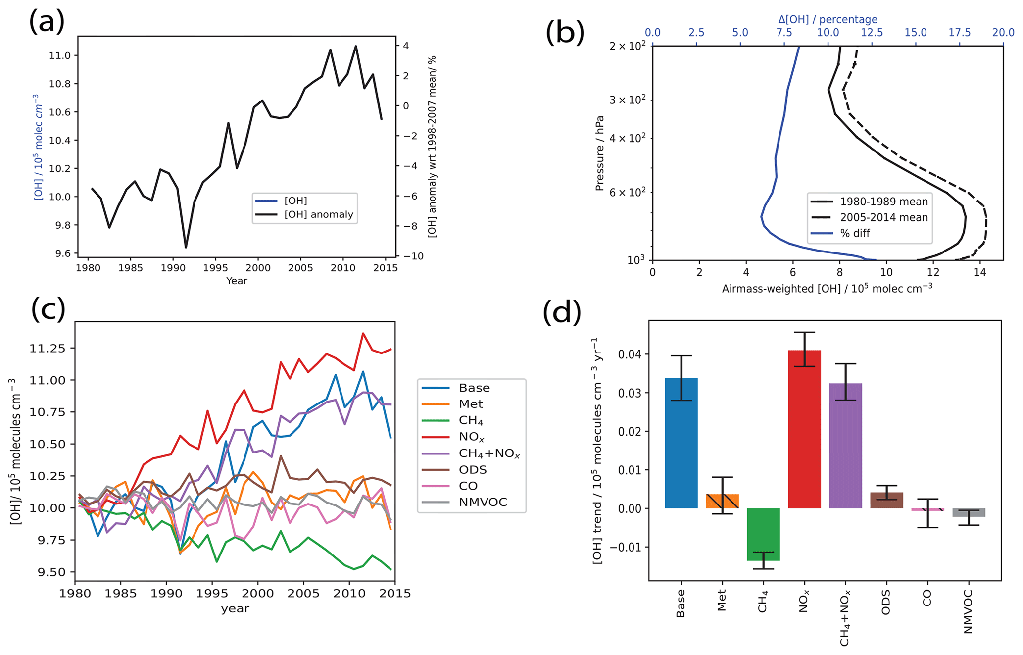
Figure 2 Tropospheric air-mass-weighted [OH] (a) time series for the Base run and the anomaly with respect to the 1998–2007 mean from 1980 to 2014, (b) 10-year global area-weighted air-mass-weighted mean [OH] at various altitudes for 1980–1989 (solid black line) and 2005–2014 (dotted black line) and the percentage [OH] difference at each altitude (blue line), (c) tropospheric air-mass-weighted [OH] time series, and (d) trends from the Base simulation and from the sensitivity simulations with all (Met) and individual short-lived emissions held constant at 1980 levels. For panel (b), error bars for the 1980–1989 and 2005–2014 means represent ±1 standard deviation about the 10-year mean at each pressure level. For panel (d), trends are calculated using the Theil–Sen method, and error bars show the 95 % confidence interval. Bars are hashed when no significant trend is detected at the 95 % level using the Mann–Kendall test. From panel (a), tropospheric air-mass-weighted [OH] has increased by ∼5 % from 1980 to 2014 in the Base simulation. As seen in panel (b), the increase in [OH] occurs throughout the depth of the troposphere, with the largest increase seen from the surface to the lower troposphere, and this could suggest that the increasing [OH] trend is driven by mainly surface drivers. From panels (c) and (d), we see that globally the [OH] increasing trend is driven by the combined effects of CH₄ and NO_x.

Next, we look at the sensitivity of simulated [OH] to various chemical drivers of [OH]. The simulated global tropospheric air-mass-weighted [OH] are plotted in Fig. 2c, with the individual model runs analyzed as per Sect. 2.2. As seen in Fig. 2d, the increasing non-lightning NO_x emissions caused the largest positive [OH] trend of 0.041±0.004 molec. cm⁻³ yr⁻¹ (95 % CI), while there is a small positive trend arising from decreasing ODS concentrations of 0.005±0.0015 molec. cm⁻³ yr⁻¹ (95 % CI). This suggests that the increasing non-lightning NO_x emissions of ∼30 % (Fig. 1c) have been the largest driving force behind the overall [OH] increase. However, the NO_x run overestimates the positive trend and fails to capture some of the modeled features in the Base run, suggesting the important contributions of other factors which dampen the effect of increasing non-lightning NO_x as we discuss below.

In terms of factors that contribute negatively to the [OH] trend, increasing CH₄ concentrations caused the largest negative trend of $-\mathrm{0.012}\pm \mathrm{0.02}$ molec. cm⁻³ yr⁻¹ (95 % CI), and there is also a small negative trend simulated in the NMVOC run of $-\mathrm{0.003}\pm \mathrm{0.02}$ molec. cm⁻³ yr⁻¹ (95 % CI). The “CH₄” run simulates a roughly 4 % decrease from 1980 to 2014, as seen in Fig. 2c, consistent with the increasing CH₄ concentrations seen over the period. We see that [OH] decreases from 1980 to 2000 before stabilizing up to 2007, after which it resumes its decrease. This follows the CH₄ trend, plotted in Fig. 1b, seen over this period, where CH₄ has increased from 1980 to 2000 before stabilizing up to 2007, after which it resumed its increase, such that the CH₄ burden has increased by about 16 % by 2014 compared to 1980 values. Over the 1980–2014 period, CO emissions do not contribute to the global average OH trend but induce large IAV (see Sect. 3.3) as evident in the CO simulation. This lack of OH trend is attributed to the lack of trend in CO emissions over the 35-year period as seen in Fig. 1a.

With NO_x and CH₄ identified as the main factors affecting the global [OH] trend, we conducted an additional sensitivity run accounting for their combined effects (“CH₄+NO_x”). As seen in Fig. 2d, the resultant OH trend of 0.032±0.05 molec. cm⁻³ yr⁻¹ (95 % CI) matches the Base run well, suggesting that the combined effects of CH₄ and NO_x drive the overall modeled [OH] trend.

Other factors, such as meteorology, that have been known to drive [OH] do not show up strongly on the global tropospheric mean analysis. This result is consistent with He et al. (2021), who used AM4.1 driven by the same emissions as this study but varied the meteorology field (model-calculated, the National Centers for Environmental Prediction, NCEP, reanalysis and Modern-Era Retrospective analysis for Research and Applications, version 2, MERRA-2, meteorology) and found that meteorology could affect the magnitudes of mean [OH] but not the trend. Nonetheless, these other factors could have important regional contributions, which we explore in the next section.

3.2 Regional tropospheric [OH] trends from 1980 to 2014

Next, we analyze the spatial patterns of the [OH] trends in order to get a more nuanced view of how [OH] is changing. In the Base run, the tropospheric air-mass-weighted column mean [OH] increases over most areas, with the largest increases over much of tropical Asia and China (Fig. 3). On the other hand, there are also areas, such as over the USA and some parts of western Europe and northern Russia, where there is a small decreasing trend, and there are areas of central Africa that sees a pronounced decreasing trend.

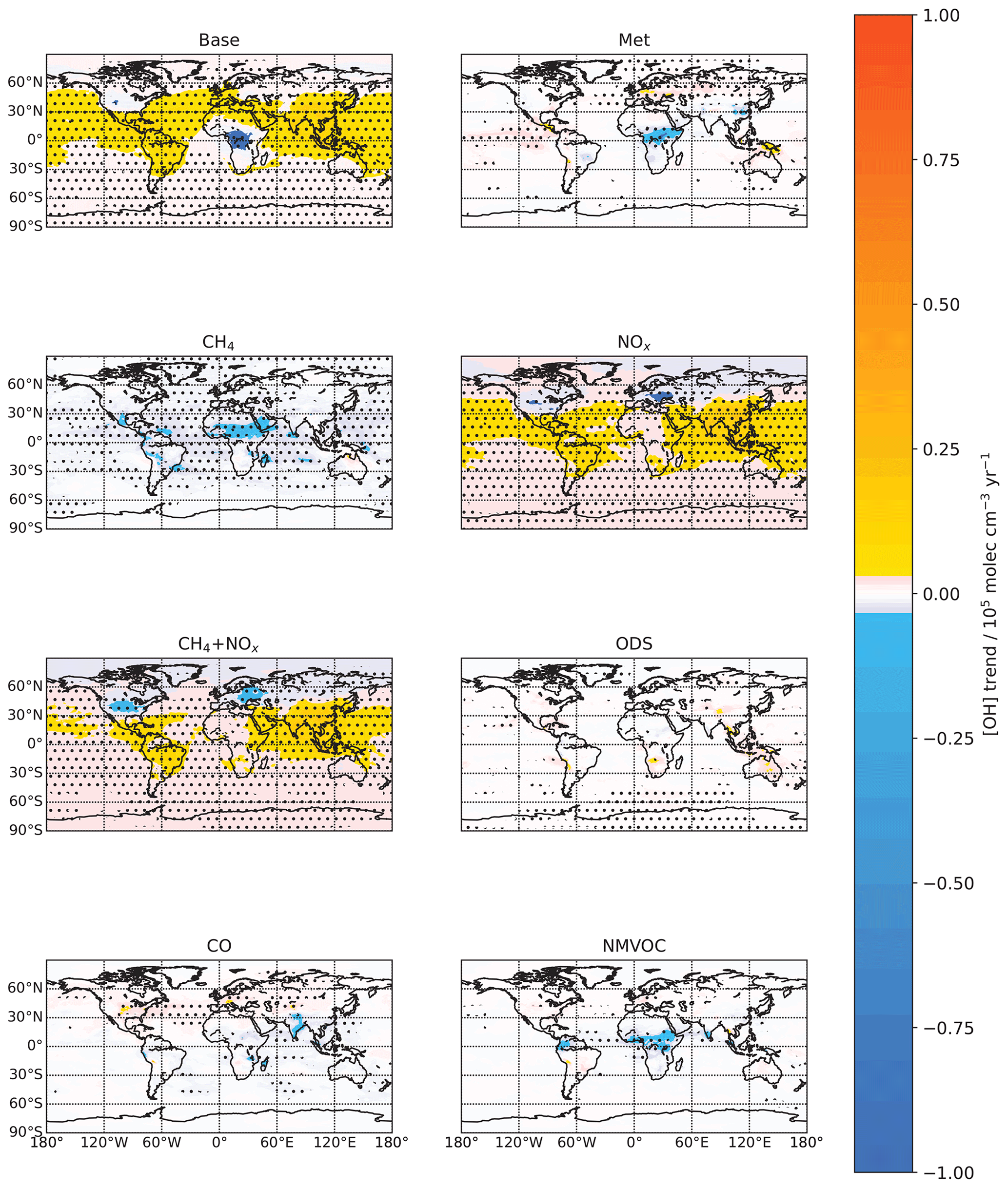
Figure 3 Trends in tropospheric air-mass-weighted OH concentrations by grid box from 1980 to 2014 for the different model runs. Trends are calculated using the Theil–Sen method. Stipples show areas where a significant trend is detected at the 95 % level using the Mann–Kendall test. In the Base run, the tropospheric air-mass-weighted column mean [OH] increases over most areas, with the largest increases over much of tropical Asia and China. These increases are also largely driven by the combined effects of non-lightning NO_x emissions and CH₄ concentrations. On the other hand, there are also areas, such as over the USA and some parts of western Europe and northern Russia, where there is a small decreasing trend, and there are areas over central Africa that see a pronounced decreasing trend.

We next see that the [OH] changes in the NO_x run are positively correlated with the changes in non-lightning NO_x emissions (Fig. 4a), which itself matches the Base run changes very well. This reinforces the earlier result that non-lightning NO_x emissions have been the main driver behind the modeled [OH] trend. However, non-lightning NO_x emissions alone seem to overpredict the decreasing trends over western Europe and northern Russia and increasing trends in the other regions. The addition of the CH₄ trend does not change the spatial pattern much, since [CH₄] increases uniformly across the surface, but it helps to bring the positive trends in line with the Base run. However, this then leads to a larger overprediction of the decreasing trends over western Europe and northern Russia.

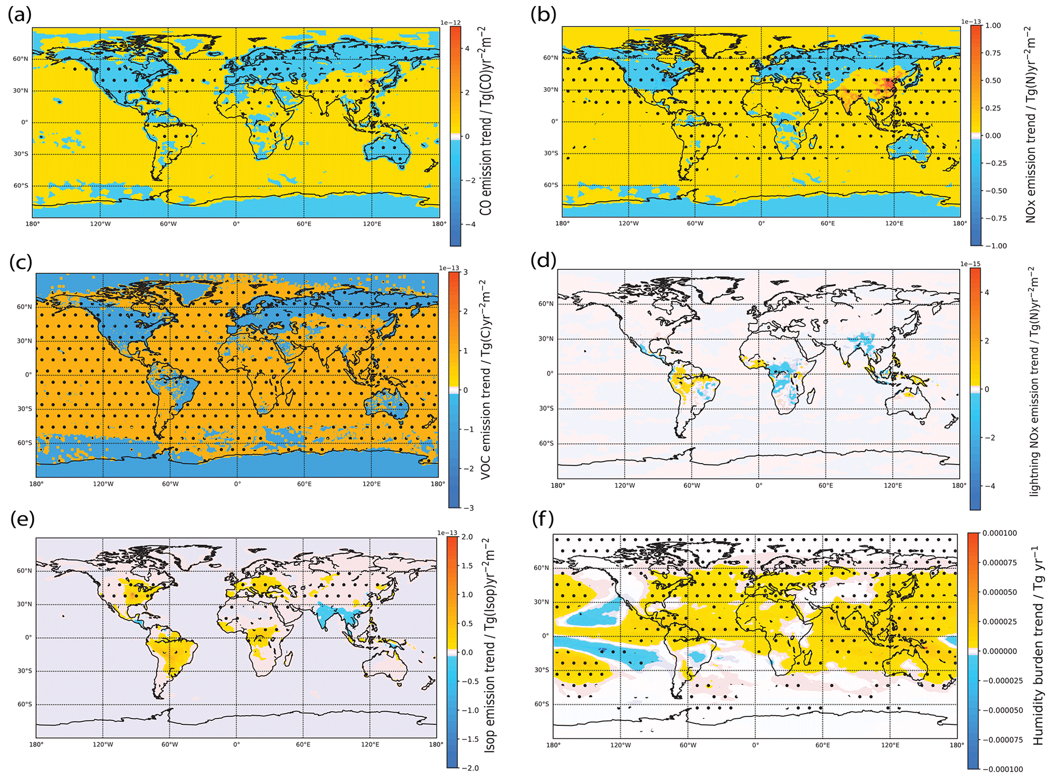
Figure 4 Spatial trends of (a) non-lightning NO_x, (b) CO, (c) NMVOC, (d) lightning NO_x, (e) biogenic isoprene emissions and (f) humidity from 1980–2014. Trends and stippling are as per Fig. 3, except for panels (a), (b) and (d), where we additionally remove stippling when the trend is below 10⁻¹⁶ Tg yr⁻² m⁻². [OH] changes in the NO_x run are positively correlated with the changes in non-lightning NO_x emissions (seen in panel a), which itself matches the Base run changes very well. Meanwhile, the CO run produces changes in [OH] that are negatively correlated with the changes in CO emissions (seen in panel b). The large negative trend over central Africa results not only from contributions from increasing CH₄ concentrations and increasing NMVOC emissions (seen in panel c), which tend to reduce [OH] by increasing chemical loss, but also from meteorology-related factors, such as lightning NO_x as seen in panel (d) and isoprene emissions as seen in panel (e). From panel (f), we see the water vapor burden has increased significantly in most regions, which tends to locally increase OH chemical production. These competing local effects on [OH] from meteorology-driven factors accounts for the absence of a globally averaged [OH] trend contribution from meteorology.

This, in turn, is largely rectified by including the effects of CO emissions. We see that the “CO” run produces changes in [OH] that are negatively correlated with the changes in CO emissions (Fig. 4b), in particular an increasing trend in [OH] over the USA, Europe and Russia associated with declining CO emissions. The addition of these effects therefore helps to dampen the effects of declining NO_x emissions and increasing CH₄ concentrations in those regions. The dampening effect of CO on NO_x effects in these particular regions is due to the large spatial correlation between the NO_x and CO emission trends as seen in Fig. 4a and b.

The large negative trend over central Africa results not only from contributions from increasing CH₄ concentrations and increasing NMVOC emissions (Fig. 4c), which tend to reduce [OH] by increasing chemical loss, but also from meteorology-related factors.

In terms of meteorology-related factors, trends in lightning NO_x have been suggested to contribute to [OH] trends (e.g., He et al., 2020; Fiore et al., 2006). From Fig. 4d it can be seen that our meteorology-driven simulation did not show significant lightning NO_x trends except for a significant negative trend over central Africa, which could further help explain the locally negative [OH] trend. Looking at other factors that could affect [OH], we see from Fig. 4e that isoprene emissions, which are interactively calculated in our model, have increased in specific regions in the meteorology-driven run, such as over the Amazon, the eastern USA, central Africa, and parts of Asia such as eastern China. Indeed, we see that these regions are associated with negative [OH] trends in the meteorology-driven run, with central Africa seeing a particularly large effect. We also see from Fig. 4f that in the meteorology-driven run the water vapor burden has increased significantly in most regions, which tends to locally increase OH chemical production. These competing local effects on [OH] from meteorology-driven factors account for the absence of a globally averaged [OH] trend contribution from meteorology.

Overall, this analysis reinforces the findings from the global average analysis of the key role of non-lightning NO_x emissions in driving the overall [OH] trends, modulated by the changes in CH₄ concentrations. However, the regional trends highlight the additional importance of CO emissions, especially in regions in the extratropical NH, as well as the importance of increasing NMVOC emissions and meteorology-driven decreases in lightning NO_x and increases in isoprene emissions in explaining the negative [OH] trend over Central Africa. Our findings from the spatial column tropospheric analysis also hold when we looked at particular pressure levels at the surface and in the middle and upper troposphere (see Fig. S1 of the Supplement).

3.3 Interannual variability

In the above analyses, we found that, in general, CH₄ and NO_x effects can largely explain the long-term [OH] trend over 1980–2014. However, the combined effects of CH₄ and NO_x alone do not account for the short-term variability in [OH] seen over this period. In particular, there are some features, such as the dip in 1992 and the dips and spikes seen between 1995 and 2000 that the “CH₄+NO_x” run misses. As seen in Fig. 5, in the global average there is a year-on-year change of up to about 0.4 molec. cm⁻³ yr⁻¹, with 13 out of the 34 years after 1980, or about one-third of the years, showing a negative year-on-year change.

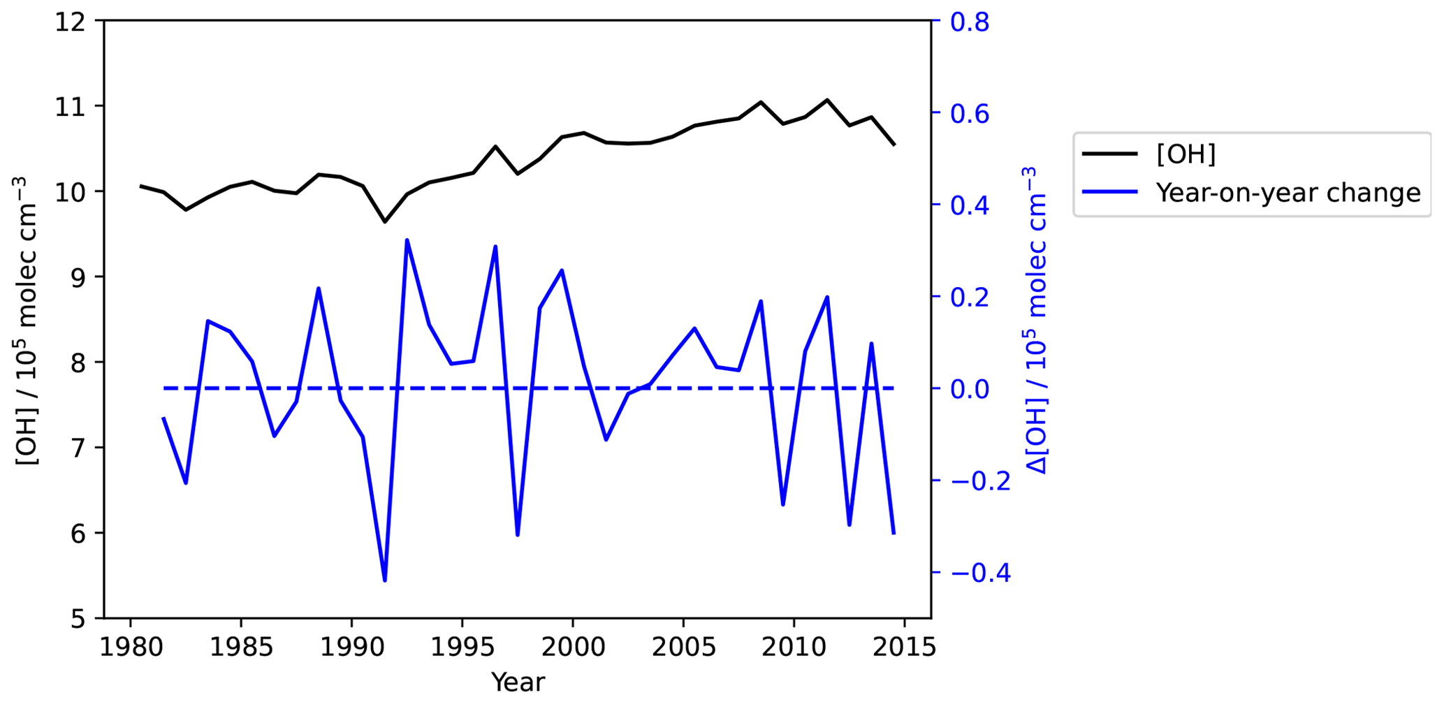
Figure 5 Base OH concentrations plotted on the left-hand y axis (black) and year-on-year changes plotted on the right-hand y axis (blue). In the global average there is a year-on-year change of up to about 0.4 molec. cm⁻³ yr⁻¹, with 13 out the 34 years after 1980, or about one-third of the years, showing a negative year-on-year change. The global IAV is driven by IAV in meteorology-related factors and CO emissions.

We see from Fig. 2c that the Base and meteorology-driven runs are positively correlated, with a Pearson correlation coefficient of r=0.82. As summarized in Sect. 1, meteorology can affect [OH] in various ways. We further see also that the CO run (pink line) also exhibits variability features that are also seen in the Base run. This could be related to variability in biomass burning, as pointed out by Holmes et al. (2013).

3.4 OH production and loss terms

3.4.1 Chemical budget terms in the base run

We first look at how the proportions of each of the production and loss terms evolves with time from 1980 to 2014 in the Base run, as shown in Fig. 6a and b. Firstly, we see that the relative proportions stay roughly constant throughout the time period, suggesting that all of the reaction terms have increased in tandem with the total. In terms of the biggest changes, we see that, for OH production terms, the primary production term has increased in proportion by the largest amount (+0.5 %), followed by small increases in the NO_x and O₃ recycling reactions (0.1 % each) at the expense of the other two terms. Meanwhile for the OH loss terms, the CO loss reaction sees quite large variability, especially from 1990 to 2000, and decreases by 1.1 % overall. The CH₄ loss reaction increases by 0.9 % overall. Comparing the production values with Table 1 of Lelieveld et al. (2016), the percentages are roughly consistent. However, our model seems to have a larger proportion of primary production (42 %) compared to Lelieveld et al. (2016) (33 %). Looking at the loss reactions, we have a lower proportion of NMVOC loss (20 % compared to 29 %) and also a higher loss to HO_y (25 % compared to 18 %).

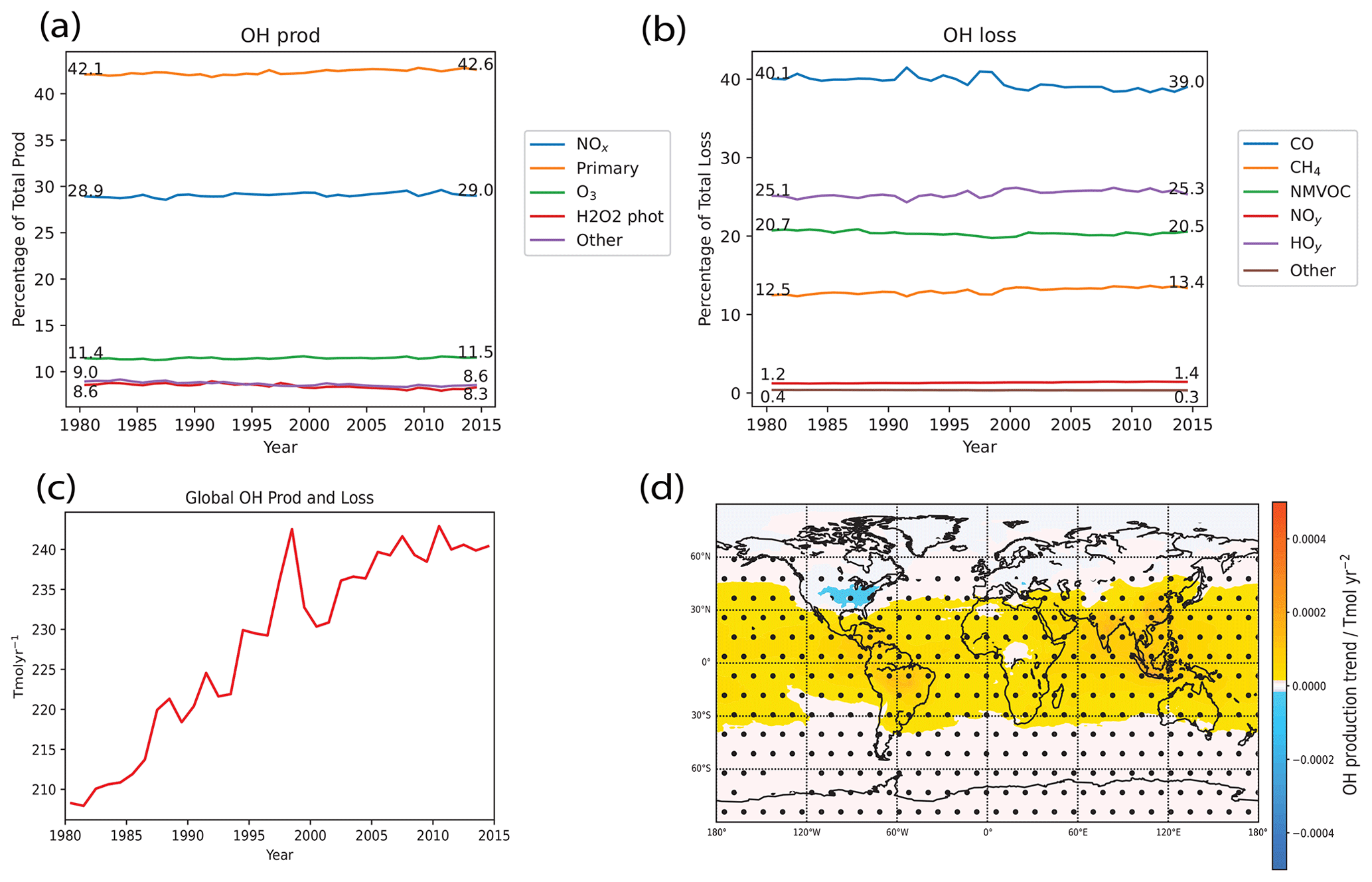
Figure 6 Tropospheric air-mass-weighted OH chemical production and loss terms in the Base run. (a) Evolution of the proportion of each production reaction with respect to the total and (b) the same but for loss reactions instead. (c) Time evolution of global total production and loss terms (curves overlap because OH is in pseudo steady state). (d) Spatial air-mass-weighted tropospheric OH chemical production trend over the 1980–2014 period, with stippling and trends as per Fig. 3. From panels (a) and (b), we see that the relative proportions stay roughly constant throughout the time period, suggesting that all of the reaction terms have increased in tandem with the total, and the values are roughly consistent with Table 1 of Lelieveld et al. (2016). From panel (c), both global tropospheric air-mass-weighted OH production and loss have increased by about 14 % by 2014 compared to 1980, showing a clear trend. We also see some IAV throughout the period, with year-on-year changes of up to 2 %. Relating these results to the earlier findings, where we saw an increasing [OH] trend, the increasing trend in both production and loss (as they balance each other in steady state) should therefore be driven by an increasing trend in production, and that in turn should be associated with the net NO_x and CH₄ effects. Meanwhile, the IAV observed in the OH concentrations should also be associated with the IAV seen in the production and loss, and this in turn should be affected by meteorological factors, factors that are driven by meteorology like lightning NO_x and biogenic VOC emissions and CO emissions. From panel (d), we see that spatial chemical production trends matches the spatial [OH] trend plot for the Base run in Fig. 3, suggesting again the role of chemical production (and loss) in driving [OH] trends.

We next look at the chemical budget terms in the Base model run. From Fig. 6c, we see that global tropospheric air-mass-weighted OH production and loss match closely with one another, consistent with the pseudo steady-state assumption. Both have increased by about 14 % by 2014 compared to 1980, showing a clear trend. We also see some IAV throughout the period, with year-on-year changes of up to 2 %. Relating these results to the earlier findings, where we saw an increasing [OH] trend, the increasing trend in both production and loss (as they balance each other in steady state) should therefore be driven by an increasing trend in production, and that in turn should be associated with the net NO_x and CH₄ effects. Meanwhile, the IAV observed in the OH concentrations should also be associated with the IAV seen in the production and loss, and this in turn should be affected by meteorological factors, factors that are driven by meteorology like lightning NO_x and biogenic VOC emissions and CO emissions. We delve into these hypotheses further in the following subsections when we do a sensitivity analysis for the budget terms.

Lastly, Fig. 6d shows the spatial plot of OH production trends from 1980 to 2014 for the Base run. We see that it matches the spatial [OH] trend plot for the Base run in Fig. 3, suggesting again the role of chemical production (and loss) in driving [OH] trends.

3.4.2 Chemical budget term sensitivity analysis

We next look at how these budget terms are affected by the input emissions by doing a sensitivity analysis using our model runs, by analyzing the sensitivity simulations involving each emissions driver and the meteorology-driven simulation. We focus our attention on the major terms represented in the budget. For production terms, we look at the primary production as well as secondary production via NO_x and O₃, together accounting for ∼84 % of total production. For loss terms, we focus on loss via CO, HO_y and CH₄, accounting for ∼78  % of total loss. Unfortunately, we did not have enough model diagnostics to study loss to NMVOCs, and this is left as potential future work. From the earlier analyses, the NMVOC-related budget term is unlikely to play a large role in affecting the global [OH] trend, even though it may have a regional role. Also, while analyzing the changes in these budget terms, we note that, due to the fact that [OH] is in pseudo steady state, we will always have total production and loss approximately balancing at all times. This means that a change in production can precede a change in loss or vice versa. To disentangle the effects, we have to rely on our physical understanding of the underlying chemistry and can take cues from how [OH] itself is changing.

Since our analysis in Sect. 3.1 showed the dominant role of NO_x in driving [OH] increases over the 1980–2014 period, we focus here on NO_x. From Fig. 7c, we see from the red line that increasing NO_x emissions have led to an increase in OH recycling from NO_x. This is to be expected, as the increasing NO_x emissions as seen in Fig. 1c drive an increase in the tropospheric NO_x burden (see Fig. S2a). This therefore increases the NO_x reaction recycling rate from Reaction (R3), acting to increase the partitioning of HO_x into OH. NO_x emissions have also caused an increase in the other major production terms. We can understand this via the impact of NO_x emissions on tropospheric O₃. Increases in NO_x emissions have driven the increasing trend seen in tropospheric O₃ burden (see Fig. S2b), with the increase of ∼30 % in non-lightning NO_x emissions leading to a ∼10 % increase in O₃. This suggests that the atmosphere as a whole is limited in terms of NO_x with respect to ozone production, with ozone production occurring via Reactions (R8)–(R10). This is consistent with other studies, e.g., Lawrence et al. (2003), who found that the lofting of surface NO_x drove significant increases in O₃ production over the tropospheric column. The increasing O₃ concentrations lead to an increase in primary production via Reactions (R1)–(R2). The increasing O₃ concentrations also lead to enhanced OH recycling via O₃ through Reaction (R4), which further partitions HO_x into OH. Murray et al. (2013) previously found that lightning NO_x influenced both primary and secondary production, and we show here that non-lightning surface NO_x emissions also have the same effect in our model. The increased OH production as a result of NO_x emissions then leads to an increase in [OH]. As loss fluxes are proportional to [OH], this in turn then leads to increased OH losses (as seen in Fig. 7b, d and f), eventually keeping OH in pseudo steady state.

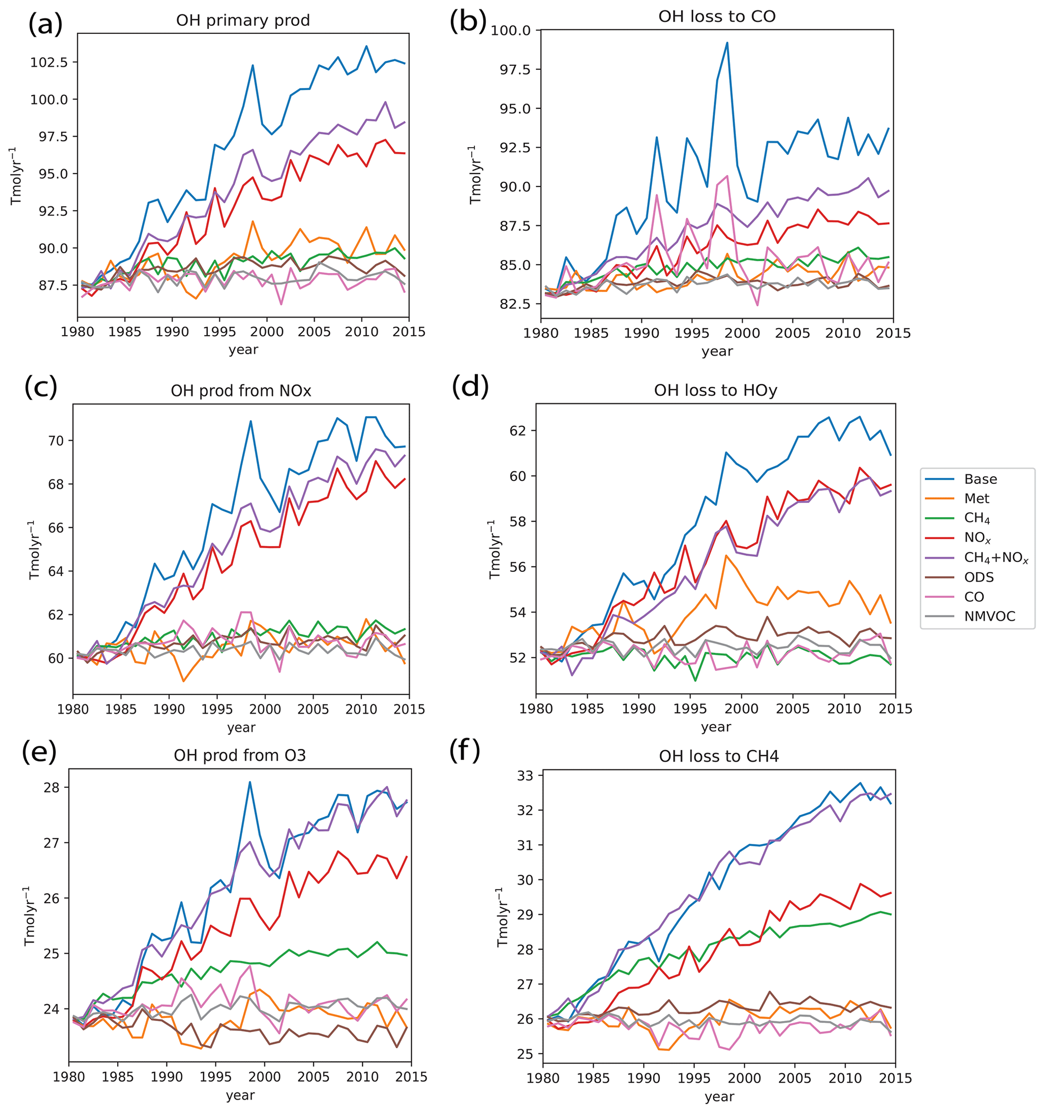
Figure 7 OH chemical production and loss budget terms for the different model runs. Panels (a), (c) and (e) show the production terms, accounting for ∼84 % of total OH production. Panels (b), (d) and (f) show the loss terms and account for ∼78 % of total OH loss. Globally, increasing NO_x emissions have led to increasing primary and secondary OH production, while increasing CH₄ concentrations have led to increased OH loss via reaction with CH₄ that is offset by increased secondary OH production due to the increase in tropospheric O₃.

Next, we look at the impacts of CH₄, which we found to suppress the increasing [OH] trend. We first see the primary effect of increased CH₄ in depleting OH in Fig. 7f. Furthermore, oxidation of CH₄ via Reaction (R7) eventually leads to the production of CO (see Fig. S2c), which then leads to a small increase in OH loss via CO in Fig. 7b. However, as CH₄ is a tropospheric ozone precursor, such as via Reactions (R8)–(R10), the increase in CH₄ also leads to increased tropospheric O₃ (see Fig. S2b), thereby slightly enhancing primary production and OH recycling via O₃ as well. Hence, this could explain why the overall net negative effect of CH₄ on [OH], which includes a mixture of enhanced losses and production, is smaller. Furthermore, we see in Fig. 7f that the NO_x run also contributes roughly equally to the OH loss due to chemical reaction with CH₄, and this further highlights the importance of changes in OH production associated with NO_x.

Lastly we look at the impacts of CO, which we found to have a regional effect on the [OH] trend. As identified earlier in Fig. 3, the main region where CO emissions have affected the [OH] trend is in some regions in the extratropical NH, such as the eastern USA and western Europe, where a decrease in CO emissions led to an increase in [OH], and in South Asia and eastern China, where an increase in CO emissions led to a decrease in [OH]. As seen for the CO run in Fig. 8, regions of decreasing CO emissions see decreasing OH loss via reaction with CO and hence an increase in [OH], and vice versa. However, comparing the Base and NO_x runs, we also see that the base OH loss flux to CO is also driven by the [OH] changes associated with the NO_x run, and this again highlights the importance of changes in OH production associated with NO_x.

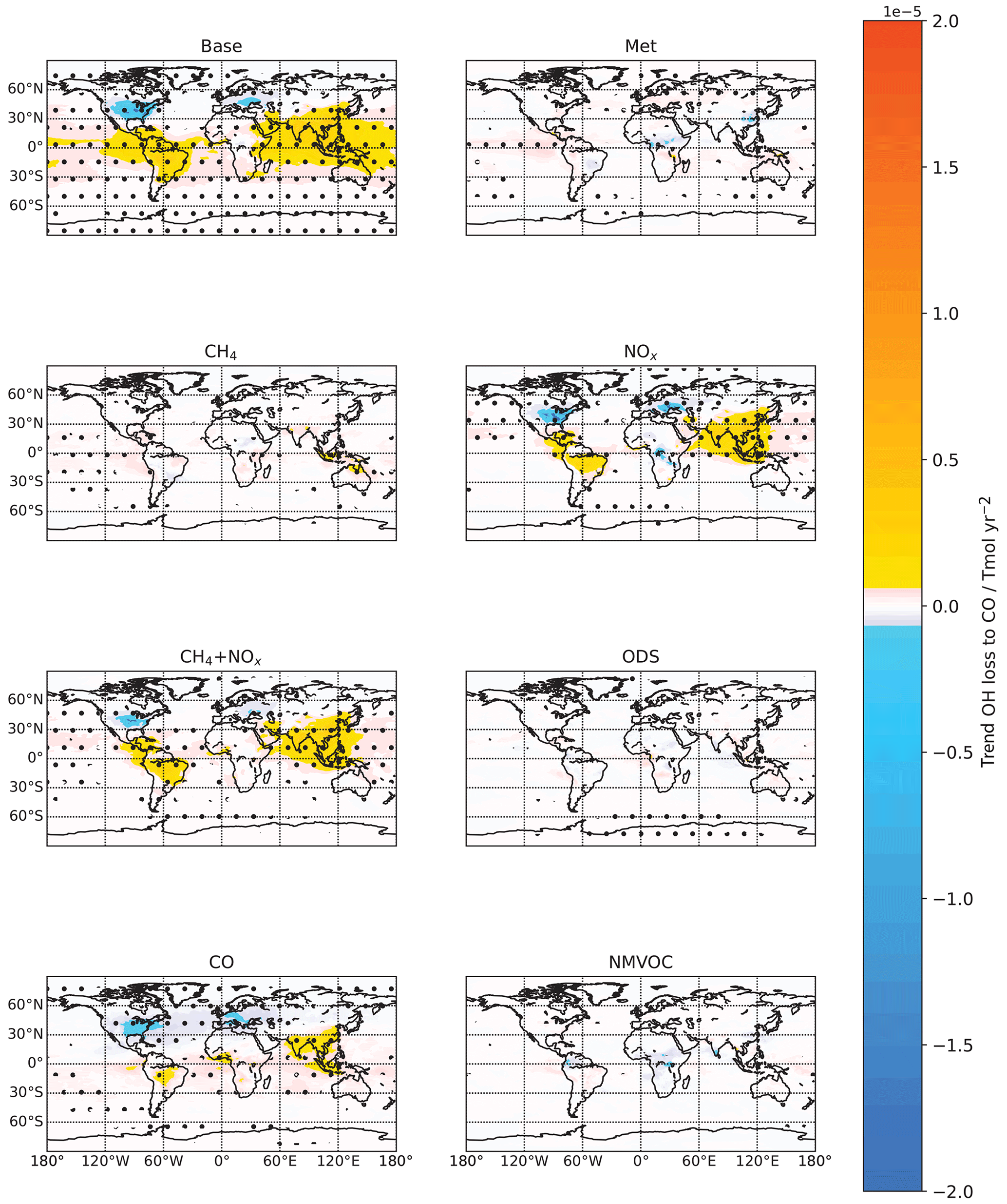
Figure 8 Tropospheric air-mass-weighted OH loss flux to reaction with CO spatial trends from 1980 to 2014 for the different model runs. Trends and stippling are as per Fig. 3. Regions of decreasing CO emissions see decreasing OH loss via reaction with CO and hence an increase in [OH] (as seen in the CO run in Fig. 3) and vice versa.

Additionally, we find that meteorology plays an important role for IAV in OH primary production, while CO emissions are more important for IAV in the OH loss flux to CO. The former is evident from Fig. 9, which shows that OH primary production is strongly correlated with changes in specific humidity (q) (Pearson correlation coefficient r=0.90) which itself is strongly correlated with temperature (r=0.96). For the latter, as seen in Fig. 10a, CO emissions are positively correlated with OH loss to CO in the Base run (r=0.69). This thereafter drives overall IAV in total loss and production. As seen in Fig. 10b, where we plot the year-on-year changes in [OH] on the left-hand y axis (black), as well as the year-on-year changes in total OH production and loss and that of the OH loss to CO on the right-hand y axis (blue), we first notice that the OH year-on-year production or loss change (solid blue) is highly correlated with that of the OH loss to CO (dotted blue) with a Pearson correlation coefficient r=0.94, suggesting that the OH loss to CO is indeed driving the IAV seen in total production or loss. The year-on-year change in production or loss is in turn anti-correlated with the year-on-year change in OH, with a Pearson correlation coefficient $r=-\mathrm{0.36}$.

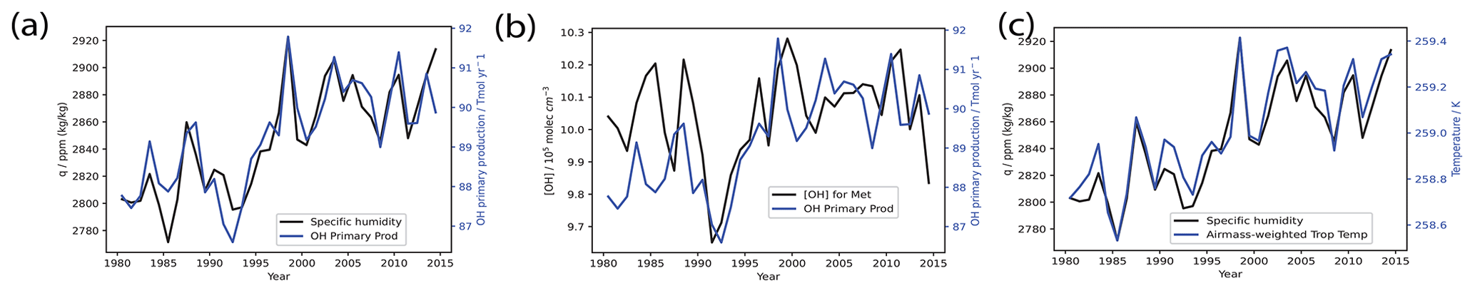
Figure 9 OH primary production and [OH] in the meteorology-driven (Met) run. Panel (a) shows the comparison between specific humidity (left-hand y axis, black) and OH primary production (right-hand y axis, blue) in the meteorology-driven run, panel (b) shows the [OH] (left-hand y axis, black) compared with OH primary production (right-hand y axis, blue), and panel (c) shows the comparison between specific humidity (left-hand y axis, black) and tropospheric air-mass-weighted air temperature (right-hand y axis, blue). Meteorology plays an important role for IAV in OH primary production, with OH primary production being strongly correlated with changes in specific humidity (q) (r=0.90), which itself is strongly correlated with temperature (r=0.96).

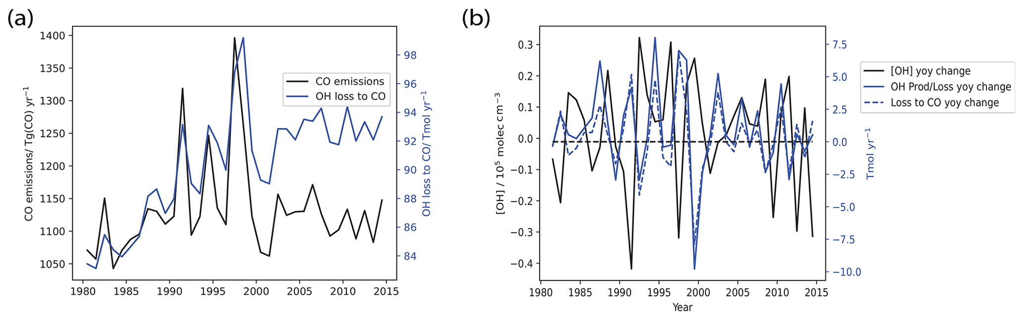
Figure 10 Plots of (a) OH loss to CO with CO emissions, and (b) the year-on-year changes in [OH] together with the year-on-year changes in net OH production and those of OH loss to CO. As seen in panel (a), CO emissions are positively correlated with OH loss to CO in the Base run (r=0.69). This thereafter drives overall IAV in total loss and production. As seen in panel (b), we see that OH year-on-year production or loss change (solid blue) is highly correlated with that of the OH loss to CO (dotted blue) with r=0.94, suggesting that the OH loss to CO is indeed driving the IAV seen in total production or loss. The year-on-year change in production or loss is in turn anti-correlated with the year-on-year change in OH, with $r=-\mathrm{0.36}$.

4 Evaluation of modeled CO and NO_x

4.1 CO: comparison with satellite column and in situ surface measurements

Figure 11a shows the MOPITT and modeled CO column trends from 2001 to 2014, and Fig. 11b shows the input CO emission trends over the same time period. The MOPITT CO column generally sees significant negative trends throughout the spatial domain, consistent with results from Yin et al. (2015). However, the modeled CO columns show significant positive trends above China and India with weaker positive trends in parts of Africa and the Middle East and negative trends over most other parts of the world. The mixed modeled CO column trends mirror the CO emission trends, especially the increasing trend over China and South Asia and are in poor agreement with trends derived from MOPITT. The MOPITT and modeled CO column trends thus show a poor agreement, and when comparing the area-weighted global (60^∘ S–60^∘ N) mean 12-month rolling mean CO columns with MOPITT observations over the 2001–2014 period in Fig. 11c, we see that the model underestimates the decreasing trend seen in MOPITT, with the model trend of $-\mathrm{0.0021}\times {\mathrm{10}}^{\mathrm{18}}$ molec. cm⁻² yr⁻¹ being 5 times smaller in magnitude than the MOPITT trend of $-\mathrm{0.010}\times {\mathrm{10}}^{\mathrm{18}}$ molec. cm⁻² yr⁻¹. Comparing Fig. 11a and b, we see that the modeled CO column trends exhibit a high spatial correlation with the input CO emission trends, and thus the mismatch between observed and modeled CO column trends could point towards some deficiencies in the input emissions, which drive the high bias in CO column trends over China and South Asia and in turn lead to the general high bias globally due to transport from these regions, especially via the prevailing westerlies (Zheng et al., 2018). Zheng et al. (2019) suggest that emissions from the version of CEDS used in our study are inconsistent for China and South Asia. Whereas the version of CEDS used in this study (and other CMIP6 runs) suggests rapidly increasing anthropogenic CO emissions from China and South Asia, Zheng et al. (2019) instead found a decreasing trend for China and a modestly increasing one for South Asia. Elguindi et al. (2020) compared regional bottom-up inventories, global bottom-up inventories which include CEDS, and top-down estimates, and they also found that CEDS (and other global bottom-up inventories) showed an increasing trend that was larger than seen in regional inventories and top-down emissions. They further point out that, for these countries, which are experiencing rapid changes in their economies, technology and environmental policies, the reason for biases in the global bottom-up inventories is that they may lack the latest data about regional activity and emission factor changes, and thus in these cases using regional or top-down inventories might reduce biases.

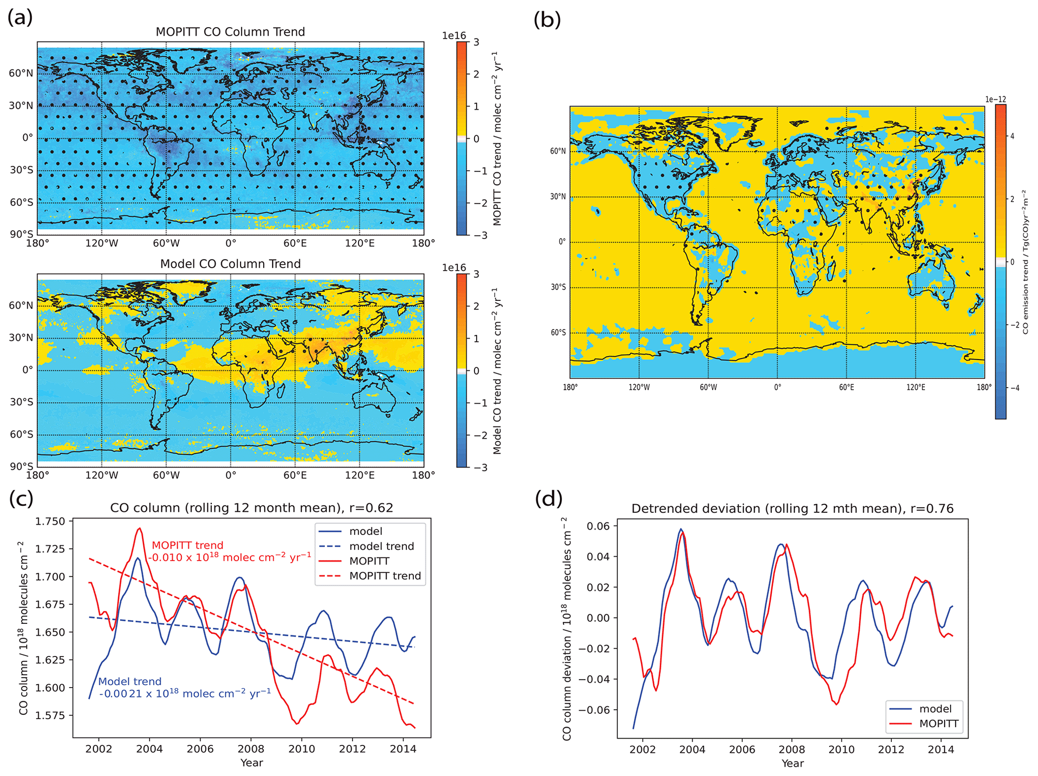
Figure 11 (a) Model comparison of annual mean CO column trends with MOPITT observations over the 2001–2014 period, (b) CO emission trends over the 2001–2014 period, (c) model comparison of area-weighted global (60^∘ S–60^∘ N) mean 12-month rolling mean CO columns with MOPITT observations over the 2001–2014 period and (d) model comparison of area-weighted global (60^∘ S–60^∘ N) 12-month rolling mean detrended CO columns with MOPITT observations over the 2001–2014 period. Trends and stippling in panels (a) and (b) are as per Fig. 3. For panel (c), the dotted lines represent the linear trend line as calculated using the Theil–Sen method. The MOPITT CO column generally sees significant negative trends throughout the spatial domain. However, the modeled CO columns show mixed trends which mirror the CO emission trends as seen in panel (b), especially the increasing trend over China and South Asia, and are in poor agreement with trends derived from MOPITT. We can also see from panel (c) that the model underestimates the negative trend seen in MOPITT. However, from panels (c) and (d), we see that the model captures the MOPITT IAV well, with Pearson correlation coefficient of r=0.62 and r=0.76 for the raw and detrended time series, respectively.

There are various implications of the model–observation mismatch. Given what we understand about how CO affects modeled [OH] in the GFDL AM4.1 from our earlier analyses, we could suspect that, in places where we underestimate the decreasing trend, we could be underestimating the [OH] increase due to decreasing CO. Meanwhile, in those areas where we model a CO increase when observations suggest a decrease instead, we may be modeling an [OH] decrease due to increasing CO in those regions, as opposed to an [OH] increase due to decreasing CO. Overall, this means that, globally, we could be underestimating the [OH] increase over the 2001–2014 period.

We next evaluate the IAV captured in the model against that observed from MOPITT, by comparing the area-weighted global (60^∘ S–60^∘ N) mean 12-month rolling mean CO columns with MOPITT observations over the 2001–2014 period in Fig. 11c and the detrended series in Fig. 11d. We see that even though the model fails to capture the decreasing CO column trend, the model captures the IAV well, with the Pearson coefficient r=0.62 and r=0.76 for the raw and detrended time series, respectively. Given that the main driver of our modeled CO IAV comes from the biomass burning emission inventory used, this could rule out the biomass burning emission inventory used as a cause of the model–observation mismatch in CO column trend. Furthermore, given the prominent role that CO plays in driving the modeled [OH] IAV, our findings here also suggest that our model is capturing the [OH] IAV due to CO well from 2005–2014.

4.2 NO_x: comparison of tropospheric NO₂ column with OMI

Figure 12a shows the annual mean OMI tropospheric NO₂ column processed by Goldberg et al. (2021) and modeled NO₂ column trends from 2005 to 2014, and Fig. 12b shows the input NO_x emission trends over the same time period. We see that there is general agreement between the emissions and the model tropospheric NO₂ column. Also, both show significant positive trends over South Asia and eastern China and significant negative trends over the eastern USA and western Europe. These are in turn also consistent with the OMI tropospheric NO₂ column observations (the OMI observations over the remote ocean are likely to have large errors due to the observational detection limit.) From the literature, Miyazaki et al. (2017), who looked at an assimilation of multiple satellite datasets, including the OMI NO₂ column, obtained a global non-lightning NO_x emission from 2005 to 2014 of a roughly constant value of 47.9 TgN yr⁻¹. This also agrees well with the emissions inventory used in our model, as shown in Fig. 1c, where, even though we are biased slightly high (about 8 % higher), our global NO_x emissions are also stable from 2005 to 2014. Overall, these findings lend confidence in our model NO_x trends from 2005 to 2014.

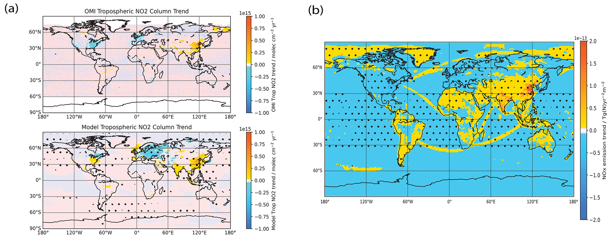
Figure 12 (a) Model comparison of annual mean tropospheric NO₂ column trends with OMI tropospheric NO₂ observations processed by Goldberg et al. (2021) over the 2005–2014 period. (b) NO_x emission trends over the 2005–2014 period. Trends and stippling are as per Fig. 3. We see that there is general agreement between the emissions and the model tropospheric NO₂ column. Also, both show significant positive trends over South Asia and eastern China and significant negative trends over the eastern USA and western Europe. These are in turn also consistent with the OMI tropospheric NO₂ column observations. Overall, these findings lend confidence in our model NO_x trends from 2005 to 2014.

5 Conclusions

In this study, we systematically analyzed the sensitivity of [OH] to changes in drivers of OH over the 1980–2014 period using the GFDL AM4.1 model. We attribute the [OH] changes to changes in emissions and meteorology individually as opposed to a lumped approach adopted in the multimodel study by Stevenson et al. (2020). Such a decomposition allows for a clearer mechanistic understanding of the main driving factors of either the trend or IAV. In addition, we analyzed the OH budget terms, similar to Zhao et al. (2020), tracing the individual emissions to changes in the various budget terms, which in turn affects [OH].

We found that annual mean global tropospheric air-mass-weighted [OH] has increased by ∼10 % compared to the 1998–2007 mean from 1980 to 2014, in agreement with multimodel comparisons of ESMs by Stevenson et al. (2020), and it has furthermore has increased by ∼5 % in 2014 compared to 1980, in agreement with multi-model studies such as ACCMIP (Naik et al., 2013) and CCMI (Zhao et al., 2019). This modeled increasing [OH] trend, especially post-2007, is in contrast with the absence of change (e.g., Nicely et al., 2020; Patra et al., 2021) or decreasing [OH] (e.g., Rigby et al., 2017; Turner et al., 2017) derived from observationally constrained inversion methods.

In our model, the increasing trend in [OH] is caused by the net effects of increasing NO_x emissions, which increases [OH] via both primary and secondary [OH] production, balanced by the increase in CH₄ concentrations, which tend to consume OH. The combined effects of NO_x emissions and CH₄ concentrations can account for the spatial distribution of the [OH] trends as well. These findings agree with other studies, such as Naik et al. (2013), who also suggested the importance of NO_x and CH₄ in driving the modeled [OH] trend. Locally, CO emissions, meteorology and NMVOC emissions also play an important role in driving the increasing [OH] trend, but their effects average out on the global level. Meanwhile, the observed [OH] IAV is dominated by impacts from the IAV in biomass burning CO emissions as well as meteorology.

We also found that while our model does a good job in matching MOPITT CO column IAV over the 2001–2014 period, our model does a poor job of matching MOPITT total column CO trends over the 2001–2014 period. Given that modeled column CO trends were driven by input CO emission trends, this could in turn point towards some deficiencies in the input emissions. Zheng et al. (2019) further suggest that emissions from CEDS, which is the anthropogenic CO emissions dataset used in our study, are inconsistent for China and South Asia. Whereas CEDS suggests rapidly increasing CO from China and South Asia, Zheng et al. (2019) instead found a decreasing trend for China and a modestly increasing one for South Asia. The increasing CO trends from China and South Asia, in turn, lead to higher CO levels. Additionally, we found that the modeled tropospheric NO₂ column trends qualitatively agree with OMI satellite tropospheric NO₂ column trends over the 2005–2014 period. Thus, overall, the underestimated declining trend in CO emissions in our model could mean that the actual modeled [OH] increase is larger than what was currently modeled.

Discussion

Overall, based on the current setup, the AM4.1 models an increase in tropospheric [OH] from 1980 to 2014. This is even against the backdrop of the increase in CH₄ throughout the period. As seen in Fig. 13, this causes the CH₄ lifetime with respect to OH (calculated via the global annual mean atmospheric CH₄ burden divided by annual mean CH₄ tropospheric chemical loss by OH) to decrease in the Base run by about 10 %. In the absence of other changes, one would expect the increase in CH₄ to reduce [OH], thereby further prolonging the CH₄ lifetime, which we in fact do see in Fig. 13 in the CH₄ run. Instead, we see that the increase in NO_x together with the stalling of CO has led to a greater increase in [OH] than would be expected by the increase in CH₄, such that CH₄ lifetime still continues to decrease. This helps to slow the accumulation of CH₄ in the atmosphere. If what we found in this study is true and [OH] has indeed increased, this could suggest that studies trying to derive CH₄ emissions from observed CH₄ concentrations will underestimate CH₄ emissions if they do not take into account the increasing [OH]. We acknowledge that CH₄ concentrations are prescribed on the surface in the current model setup, and this can lead to an underestimation of the surface chemical feedbacks. Including the surface feedbacks would likely amplify the modeled effects of CH₄ on [OH]. This will be further investigated in an emissions-driven run.

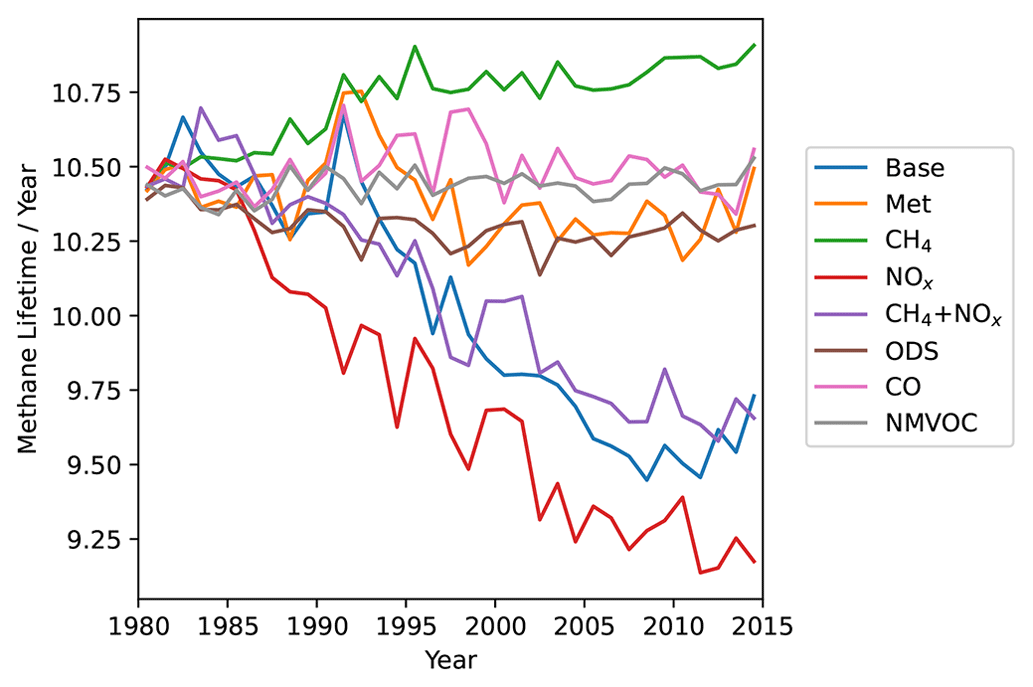
Figure 13 CH₄ lifetime with respect to oxidation by OH for the different model runs. CH₄ lifetime is calculated via the global annual mean atmospheric CH₄ burden divided by annual mean CH₄ tropospheric chemical loss by OH. CH₄ lifetime has decreased in the Base run even as CH₄ concentrations have increased driven by [OH] increases.

Also, in the future, should aggressive air quality policies cause a reduction in NO_x emissions, this could cause the [OH] to decrease, thereby further accelerating the buildup of CH₄ in the atmosphere. On the other hand, if CO emissions also decrease concomitantly, this could offset the NO_x reduction effects on [OH]. Future work could involve looking at how [OH] evolves under future scenarios, such as the Shared Socioeconomic Pathways (SSPs) formulated as part of CMIP6. In particular, future work could focus on whether NO_x and CO will still play a dominant role in the future under different scenarios of climate change as well as emissions reductions. The recent COVID-19-related large reduction in emissions in cities across the world has provided a glimpse of what could happen in future scenarios. For example, Laughner et al. (2021) found that the decrease in NO_x emissions in 2020 led to a decrease in ozone, which thereby led to a 2 %–4 % decrease in global [OH], and this could have contributed to the large [CH₄] growth rate that year. This was further corroborated by Stevenson et al. (2022) and Peng et al. (2022), who both found that about half of the large [CH₄] growth rate was attributed to the decline in [OH] due to declining NO_x. Peng et al. (2022) also additionally showed that the effect of declining NO_x emissions, which led to decreased [OH], overwhelmed the impacts of the decline of other NTCFs like CO emissions. NO_x emissions have since largely returned back to pre-pandemic levels, and this could drive [OH] increases again. Against the backdrop of the anthropogenic emission changes, the pandemic years have also seen many large wildfire events as well, and the associated biomass burning emissions could also impact [OH]. Overall, these could be interesting test cases to explore in ESMs with interactive chemistry.

In our paper, we explored the role of meteorology and input emission inventories in driving the [OH] trend during the 1980–2014 period, but, as Murray et al. (2021) points out, there are many other factors within models that could be important in driving inter- and intra-model [OH] variations, with key factors being the details of the implemented chemical scheme, which has implications on oxidation of VOCs into CO and NO_x lifetime, as well as other physical parameterizations, such as lightning NO_x altitude, which also affects NO_x lifetime. The importance of understanding the CO budget drivers and potential biases is further underscored by the existing biases present in the GFDL AM4.1, such as in the seasonal mean CO column (Horowitz et al., 2020) and the CO column trend. Nonetheless, given that we have identified various input emission drivers as playing a key role in driving the increasing [OH] trend over the 1980–2014 period, and other models participating in CMIP6 also have likely used the same anthropogenic emission inventories, our study could also serve as a motivation to do a similar sensitivity analysis in other CCMs, such as the other ESMs studied in Stevenson et al. (2020). This could help elucidate the role of emissions in driving the multi-model mean trend, and potentially further emphasize the importance of accurate short-lived climate forcer emission inventories for both climate and air quality projections (Smith et al., 2022).