the Creative Commons Attribution 4.0 License.
the Creative Commons Attribution 4.0 License.
 | 27 Apr 2023
Aerosol impacts on the entrainment efficiency of Arctic mixed-phase convection in a simulated air mass over open water
Dmitry Chechin
Regis Dupuy
Birte S. Kulla
Christof Lüpkes
Stephan Mertes
Mario Mech
Roel A. J. Neggers
Springtime Arctic mixed-phase convection over open water in the Fram Strait as observed during the recent ACLOUD (Arctic CLoud Observations Using airborne measurements during polar Day) field campaign is simulated at turbulence-resolving resolutions. The first objective is to assess the skill of large-eddy simulation (LES) in reproducing the observed mixed-phase convection. The second goal is to then use the model to investigate how aerosol modulates the way in which turbulent mixing and clouds transform the low-level air mass. The focus lies on the low-level thermal structure and lapse rate, the heating efficiency of turbulent entrainment, and the low-level energy budget. A composite case is constructed based on data collected by two research aircraft on 18 June 2017. Simulations are evaluated against independent datasets, showing that the observed thermodynamic, cloudy, and turbulent states are well reproduced. Sensitivity tests on cloud condensation nuclei (CCN) concentration are then performed, covering a broad range between pristine polar and polluted continental values. We find a significant response in the resolved mixed-phase convection, which is in line with previous LES studies. An increased CCN substantially enhances the depth of convection and liquid cloud amount, accompanied by reduced surface precipitation. Initializing with the in situ CCN data yields the best agreement with the cloud and turbulence observations, a result that prioritizes its measurement during field campaigns for supporting high-resolution modeling efforts. A deeper analysis reveals that CCN significantly increases the efficiency of radiatively driven entrainment in warming the boundary layer. The marked strengthening of the thermal inversion plays a key role in this effect. The low-level heat budget shifts from surface driven to radiatively driven. This response is accompanied by a substantial reduction in the surface energy budget, featuring a weakened flow of solar radiation into the ocean. Results are interpreted in the context of air–sea interactions, air mass transformations, and climate feedbacks at high latitudes.
- Article
(7050 KB) - Full-text XML
- BibTeX
- EndNote


The ongoing accelerated warming of the Arctic climate involves various processes and feedback mechanisms, many of which are still poorly understood. Recent research has highlighted the role of warm-air intrusions (Bennartz et al., 2013; Pithan et al., 2018) as well as the lapse rate feedback (Pithan and Mauritsen, 2014; Lauer et al., 2020). Clouds play a sophisticated role in these mechanisms. For example, cloud presence in warm-air intrusions significantly affects the downward longwave radiative flux at the surface (Liu et al., 2018). Radiative cooling at the liquid cloud top also causes turbulence, which in turn drives entrainment that counteracts larger-scale subsidence, together maintaining the low-level inversion and lapse rate (e.g., Neggers et al., 2019). Arctic clouds form through a variety of processes acting on a broad range of scales (e.g., Mauritsen et al., 2011; Morrison et al., 2012). Gaining further insight has motivated intense research on Arctic air masses and clouds, including a number of field campaigns at high latitudes (Perovich et al., 1999; Tjernström et al., 2012; Knudsen et al., 2018; Wendisch et al., 2019; Shupe et al., 2021).
This study focuses exclusively on mixed-phase convective clouds in relatively stagnant air masses over open water. Previous studies on marine cold-air outbreaks (CAOs) have shown that the strong surface–atmosphere temperature difference over open water can drive intense cloudy convection, which is efficient in vertically mixing the lower atmosphere (Chlond, 1992; Atkinson and Wu Zhang, 1996; Müller et al., 1999; Gryschka and Raasch, 2005; Fletcher et al., 2016). In comparison, weaker convection in more stagnant air masses has received far less attention. However, such air masses occur frequently and might occur even more in a warmer future Arctic featuring a slower polar jet stream (Screen et al., 2013; Barnes and Screen, 2015). Slow-moving air masses also have much more time to adjust to local conditions, which potentially makes the vertical mixing more efficient. Finally, the ongoing shift in Arctic climate is arguably strongest felt in areas where the sea ice disappears (Liu et al., 2012; Overland et al., 2014). The marine areas adjacent to the sea ice also act as gateways for injections of aerosol (Browse et al., 2014; Ito and Kawamiya, 2010), moisture, and heat (Vázquez et al., 2016; Rinke et al., 2017; Pithan et al., 2018) into the high Arctic.
These reasons motivate taking a closer look at such stagnant marine air masses, in particular concerning clouds and turbulent mixing. Recent years have seen an increased use of large-eddy simulation (LES) to study these processes, often based on Arctic field campaign data. LES can supplement the observational data record and act as a virtual research laboratory (e.g., Ovchinnikov et al., 2014). At the same time, independent measurements of mixed-phase cloud properties can be used to evaluate the simulations (Neggers et al., 2019; Kretzschmar et al., 2020; Ruiz-Donoso et al., 2020). This approach has led to demonstrable progress in understanding Arctic clouds. A few recent papers have investigated aerosol impacts on mixed-phase clouds (de Roode et al., 2019; Stevens et al., 2018). However, no LES study has yet examined these impacts in more stagnant air masses over open water near the ice edge. In addition, no LES study has yet used in situ cloud condensation nuclei (CCN) measurements at the cloud level to constrain simulations of this cloud regime.
The main science goal of this study is to use LES to gain more insight into how and to what extent aerosol variations in a slow-moving Arctic air mass over open water can modulate its transformation by low-level turbulent/convective mixing and clouds. Of particular interest are aerosol impacts on the efficiency of radiatively driven entrainment in warming the boundary layer, as well as the associated shifts in the heat budgets of the boundary layer and the surface. While the entrainment efficiency has previously been investigated for warm turbulent clouds in the subtropics (Stevens et al., 2005), this is not yet the case for mixed-phase clouds at high latitudes. What is also still unclear is how CCN concentrations might affect this efficiency (Garrett et al., 2002; Douglas and L'Ecuyer, 2021). Given the importance of low-level warming and aerosol variations in Arctic amplification, in particular in the context of the lapse rate feedback, gaining more insight into this process and its sensitivities is crucial.
To achieve these objectives a composite LES case is constructed based on the extensive data collected by the Polar 5 and Polar 6 aircraft of the German Alfred Wegener Institute in the Fram Strait during the ACLOUD campaign (Arctic CLoud Observations Using airborne measurements during polar Day) (Wendisch et al., 2019). Research flight RF20 on 18 June 2017 sampled mixed-phase clouds as embedded in a stagnant air mass off the sea ice edge. The sampled convection was significant but still relatively weak compared to typical cold-air outbreak conditions. The boundary conditions and large-scale forcings for the simulations are based on weather model data, while the initial state is based on dropsonde data as well as in situ aerosol data at the cloud level. First the control experiment will be evaluated against independent aircraft data on clouds and turbulence, seeking agreement on basic bulk properties that are well observable. Based on this control run, sensitivity tests are then performed on CCN and levels in the air mass. Compared to previous LES studies of this kind, a much broader CCN range is covered to capture the large observed variation in Arctic air masses between pristine polar and polluted continental values.
Section 2 describes details of the ACLOUD field campaign, including the weather situation, the research flights, and the observational datasets collected. The model configuration adopted in this study is described in detail in Sect. 3, including the LES code, the treatment of microphysics, the case configuration including forcings and boundary conditions, and the experimental setup. The presentation of the results is subdivided into two parts. Part I describes the basic behavior of the control experiment, including an evaluation of cloud and turbulence statistics against ACLOUD observational datasets (Sect. 4). Part II then focuses on the aerosol sensitivity experiments (Sect. 5). The obtained results are further interpreted in Sect. 6, and the main conclusions and outlook are summarized in Sect. 7.
2.1 The ACLOUD field campaign
The ACLOUD field campaign took place from 23 May to 26 June 2017 in the vicinity of Svalbard. ACLOUD and its sister campaign PASCAL (Physical feedbacks of Arctic planetary boundary level Sea ice, Cloud and AerosoL; Macke and Flores, 2018; Wendisch et al., 2019) were part of the ongoing (AC)3 research program (Arctic Amplification: Climate Relevant Atmospheric and Surface Processes and Feedback Mechanisms; Wendisch, 2017). Both campaigns focused on clouds in the lower troposphere in the northern Fram Strait during Arctic spring. ACLOUD featured collocated airborne observations (Ehrlich et al., 2019b) performed by the aircraft Polar 5 (P5) and Polar 6 (P6) of the German Alfred Wegener Institute (Wesche et al., 2016). An overview of the synoptic conditions during ACLOUD is provided by Knudsen et al. (2018). Airborne observations were made during a wide range of cloud conditions, including both stably stratified and convective regimes.
2.2 RF20
This study exclusively focuses on research flight RF20 by the P5 and P6 aircraft on 18 June 2017 (see Fig. 1). As described by Knudsen et al. (2018), on this day the mid-troposphere experienced drying. High cirrus clouds were initially present but disappeared during the day. The air mass in the Fram Strait was slow-moving and situated over relatively warm open water.
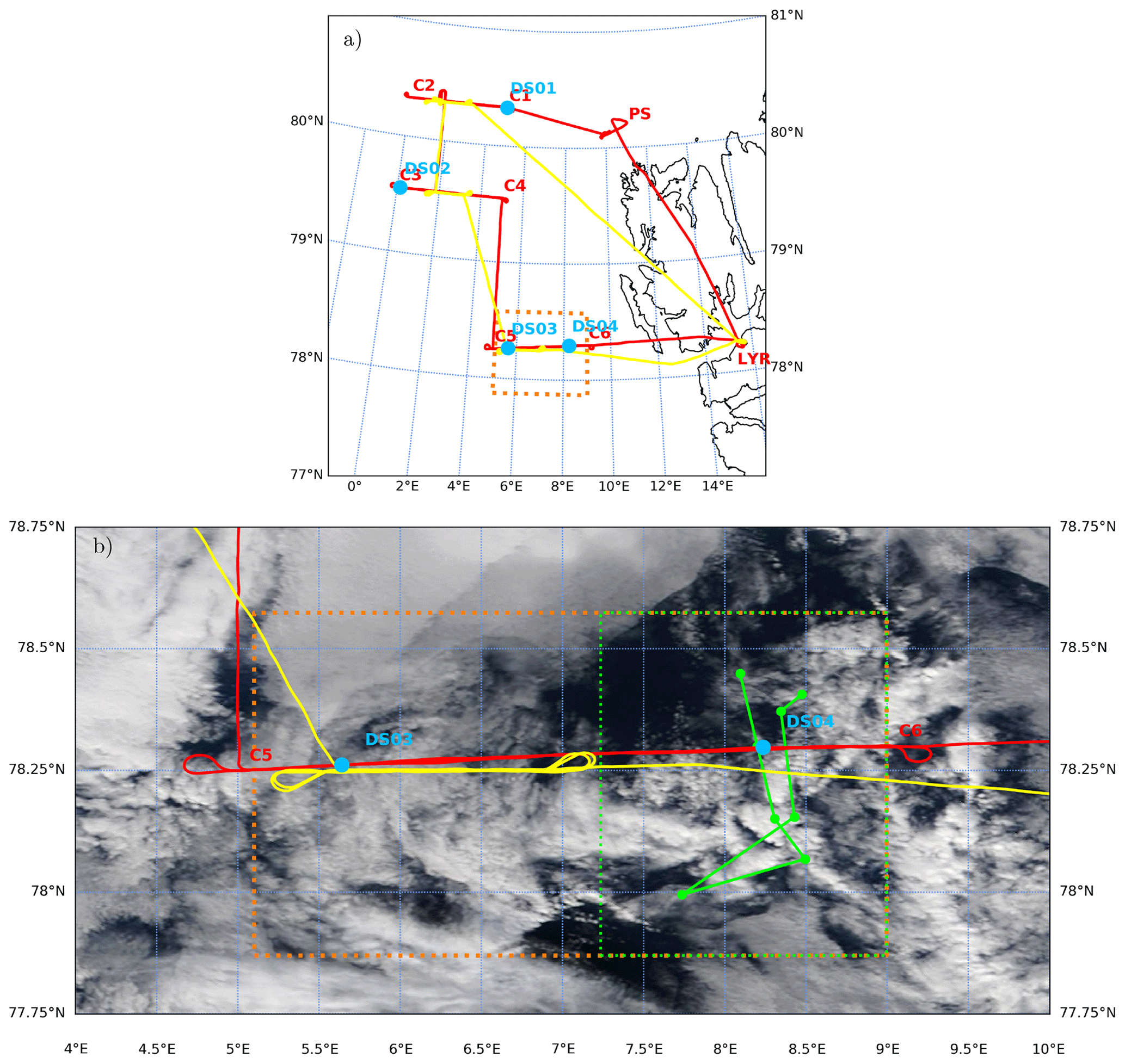
Figure 1(a) The location of the RF20 mission over Fram Strait west of Svalbard (b) with a close-up of the target area: MODIS TERRA true-color image at 250 m effective resolution during RF20 on 18 June 2017. The flight tracks of Polar 5 and Polar 6 are shown in red and yellow, respectively. For P5 the waypoints (C), RV Polarstern (PS) and Longyearbyen airport (LYR) are also indicated, with the dropsonde (DS) locations shown as blue dots. The 24 h air mass trajectory intersecting with DS04 is shown as a solid green line. The target domain including the southern racetrack section is indicated by the dotted orange box, of which the simulated part is indicated by the dotted green box. MODIS data obtained through NASA Worldview (https://worldview.earthdata.nasa.gov/, last access: 22 July 2022).
Figure 1 shows that the cloud situation in the Fram Strait as encountered by the aircraft was relatively complex. A rough north–south regional division in cloud character can be made. In the north, over the sea ice and its margin, the clouds were absent or very thin, allowing for good visibility of the sea ice from the satellite and the aircraft. In the western and middle parts of the Fram Strait the clouds were thicker but still only weakly convective, visible in Fig. 1 as vague but not completely opaque cloud patches. In the southern part the clouds were truly convective, being broken, thicker, and more opaque.
The P5 and P6 aircraft followed counterclockwise flight paths from their base at Longyearbyen airport (LYR) and visited these three regimes consecutively. This study focuses exclusively on the convective clouds in the southern areas, as sampled during the last eastbound flight leg between waypoints C5 and C6. In this section, also referred to as the “southern racetrack”, both aircraft flew back and forth between C5 and C6. While P5 doubled back once and maintained altitude above the boundary layer inversion (at about 1.5 km height), P6 doubled back twice, staying below inversion height and maintaining constant altitude for five brief flight segments. In situ in-cloud measurements were made by P6 during this period. The enhanced and targeted sampling during the southern racetrack sections, as well as the occurrence of significant mixed-phase convection, motivates adopting this area as the target domain of this study, as indicated by the orange box in Fig. 1.
2.3 Observational datasets
The observational data from the ACLOUD campaign used in this study are summarized in Table 1. Figure 2a shows detailed measurements of the clouds in the target area as obtained with the Microwave Radar/radiometer for Arctic Clouds radar on board P5 (MiRAC; Mech et al., 2019). Because of the doubling back between C5 and C6, the same cloud structure appears three times, once in each panel. Cloud top height varies significantly along the flight track in this area, which is typical of broken convective cloud fields. The maximum cloud top height is at approximately 1.4 km, which is consistent with the thermal inversion height visible in the DS04 profile (see Fig. 3a) and the Airborne Mobile Aerosol Lidar (AMALi; Stachlewska et al., 2010) measurements (also included in Fig. 2). The MiRAC flight sections between 7–8.5∘ E feature significant but narrow convective precipitation that also reached the surface. This area was visited by P5 three times, at around 16:20, 16:35, and 17:00 UTC. The DS04 dropsonde was also launched into this area. The freezing level is situated at about 350 m height, which is well below the maximum cloud top.
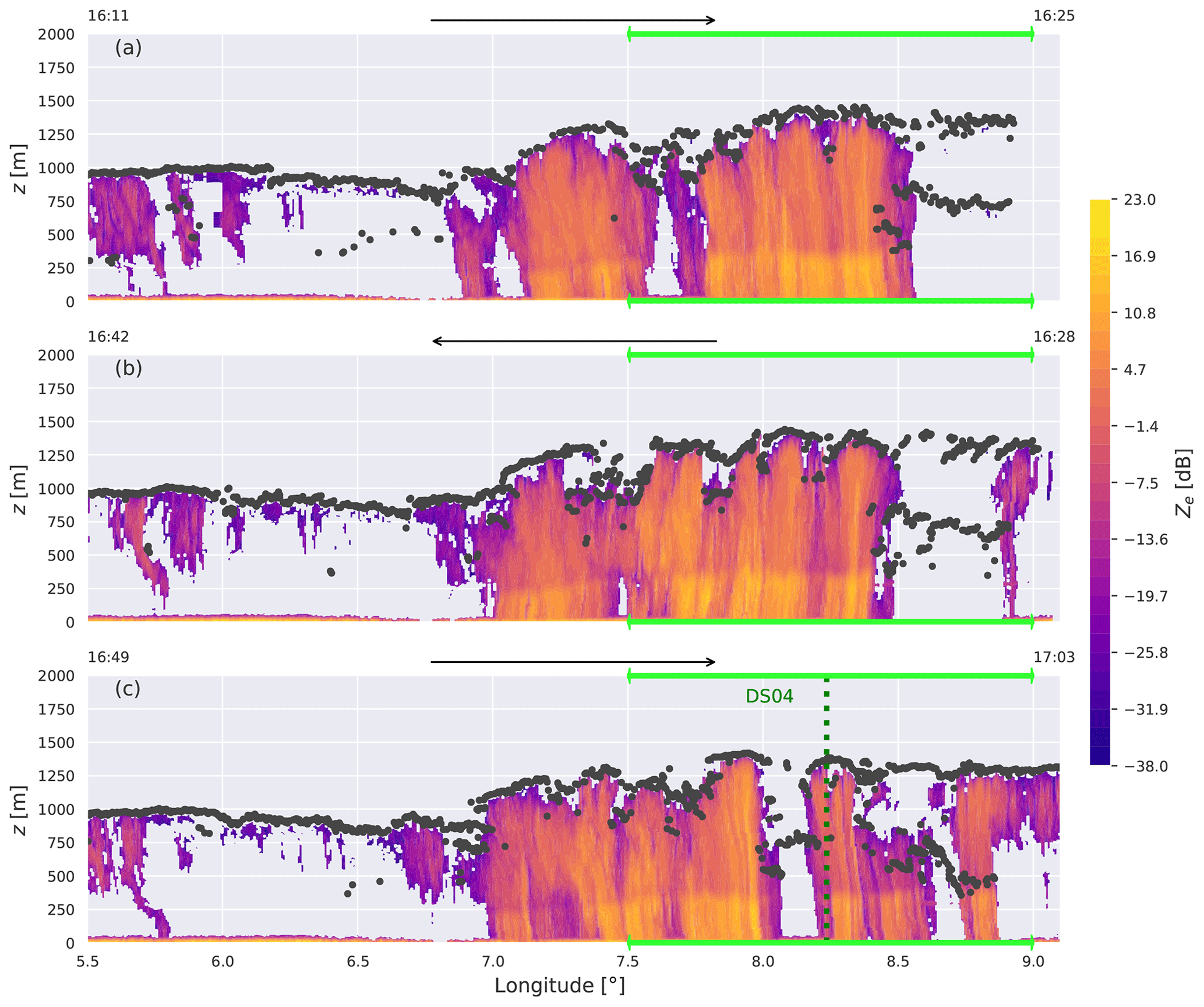
Figure 2Time–height cross section of P5 MiRAC radar reflectivity Ze during RF20 (contour shading) and the indicated liquid cloud top from AMALi (black dots). The displayed longitude range corresponds to the orange target domain as shown in Fig. 1, while the lime green horizontal line indicates the simulated domain. The black arrows indicate the flight direction of the aircraft for each leg, with the start and end times indicated at the sides. The location of the dropsonde DS04 is indicated by the dotted dark-green vertical line.
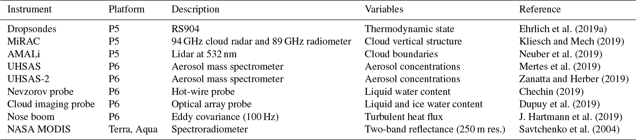
Table 1Overview of the observational datasets used in this study. Data in rows 1–7 are accessible through the PANGAEA database, while the MODIS data are available through the NASA Worldview* interface.
* https://worldview.earthdata.nasa.gov (last access: 20 July 2022).
The eastern part of the target domain that is centered around dropsonde DS04 is selected as the area to be simulated (indicated by the green box in Fig. 1 and the green line in Fig. 2). This choice is motivated by the following considerations. First, marine mixed-phase convection did occur in this area. Second, the combination of warm water and cold air implies large surface latent and sensible heat fluxes, making the near-surface convection vigorous and potentially well coupled to the cloud layer. Such convective conditions often occur in this region, for a large part controlled by the wind direction. Third, convective clouds are well resolved in large-eddy simulations. A further advantage is that the cloud-bearing low-level air mass in this area was slow-moving and almost stagnant. This is evident from (i) the dropsonde profiles of u and v (Fig. 3) and (ii) the trajectory staying in the proximity to the dropsonde location for about 24 h (Fig. 1). This broadens the time span that the simulation results can be justifiably compared to relevant measurements. The P5 and P6 aircraft visited the area between waypoints C5 and C6 multiple times, which enhances the sample size. Finally, the decision to only simulate the eastern part of the target domain is mainly based on the need to avoid averaging large-scale forcings over a too wide area so that the simulated convection remains optimally representative of the local (convective) conditions surrounding DS04.
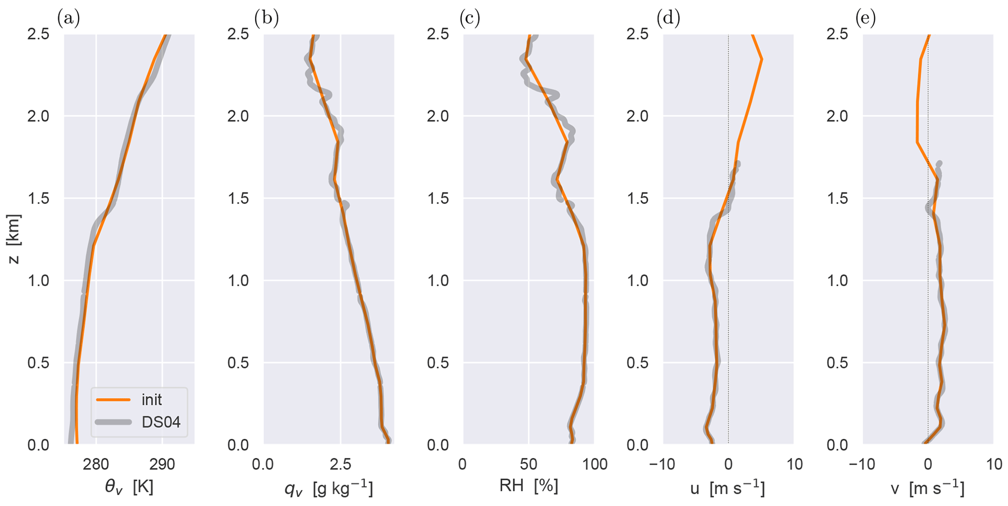
Figure 3Dropsonde profiles from RF20 of (a) virtual potential temperature θv; (b) water vapor specific humidity qv; (c) relative humidity RH; and the (d) zonal and (e) meridional wind speeds u and v, respectively. The DS04 sounding is shown in grey. The idealized initial (init) profiles are shown in orange.
The DS04 dropsonde data provide detailed insight into the thermodynamic structure of the marine boundary layer in the simulation domain. Figure 3a and b show that an inversion layer is present between 1.3–1.5 km height and can be recognized in most state variables. A well-mixed sub-cloud layer of about 350 m depth is capped by a relatively deep cloud layer, characterized by high relative humidity values and a conditionally unstable thermodynamic vertical structure. The inversion features a θv jump of about +3 K. In contrast, the jump in water vapor specific humidity qv is relatively small, indicating the presence of significant water vapor above the inversion. There is a notable gap in wind measurements between 1.6–2.5 km, where samples have been removed after quality checks.
The observational data on hydrometeor occurrence and mass as collected by P5 and P6 are used to evaluate the LES experiments. While the MiRAC and AMALi data on board P5 provide information about cloud top heights, vertical structure, and liquid water path, the Nevzorov probe on board P6 provides in situ samples of cloud liquid water content. The Laboratoire de Météorologie Physique (LaMP) cloud imaging probe (CIP) provides data on both liquid and ice water content, using a Brown and Francis (1995) mass diameter relationship on non-spherical particles only. Finally, the high-frequency (100 Hz) turbulence measurements collected by the P6 nose boom (Hartmann et al., 2018) allow for calculating (co)variances of temperature and vertical velocity in the boundary layer, even for relatively short flight segments.
A unique aspect of RF20 is the operation of two ultra-high-sensitivity aerosol spectrometers (UHSASs) on board P6, both sampling submicron-size particles (Zanatta and Herber, 2019). These instruments measured the number size distribution of particles with diameters between 60 and 1000 nm by detecting scattered laser light, using the method described in detail by Cai et al. (2008). Figure 4 shows that a relatively wide range of aerosol concentrations was encountered. The data, as documented by Mertes et al. (2019), suggest a marked difference in aerosol loading below and above the cloud layer, with the lower values found below the clouds. The availability of in situ aerosol data greatly helps to constrain the LES, given the well-known sensitivity of mixed-phase clouds to this parameter. Accordingly, the UHSAS data form the basis for the initial CCN profile as adopted in the simulations described in Sect. 3.4. We hypothesize that the removal of aerosol by precipitation is the main reason for the lower values below the clouds; if this is the case, it should also show up in the simulations.
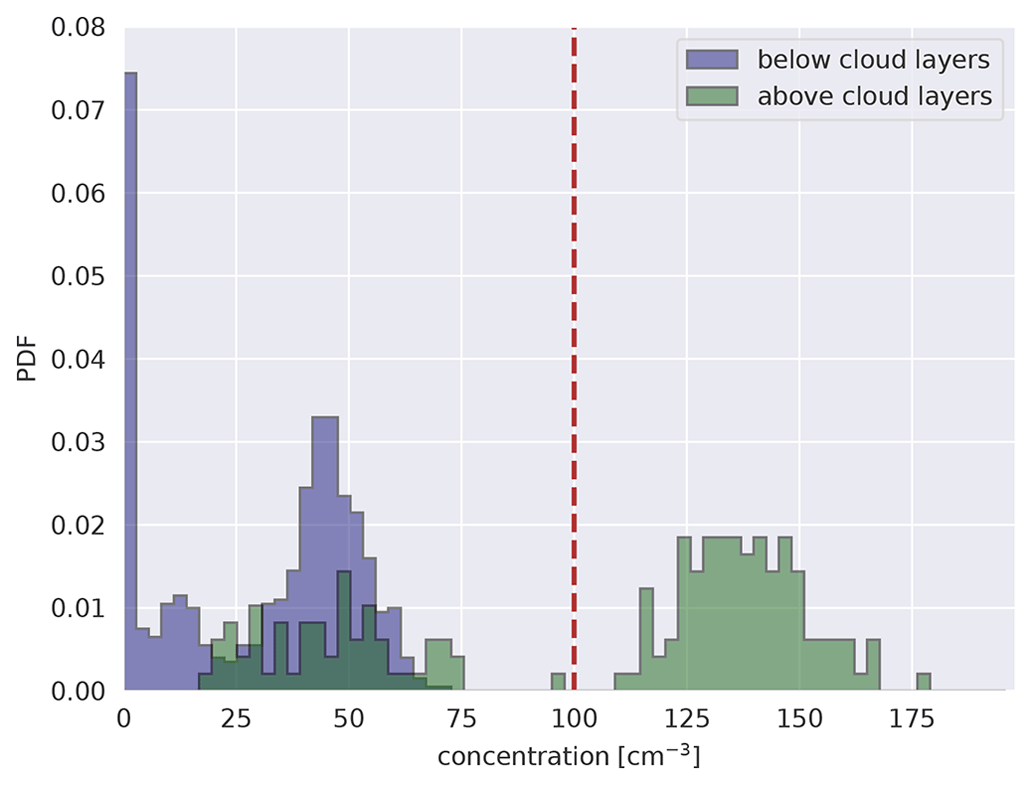
Figure 4The probability density function (PDF) of aerosol concentrations (for aerosol particles of diameters between 80 and 1000 nm) as observed by the UHSAS-2 mass spectrometer on P6 during the southern racetrack section of RF20. The southern racetrack is shown in Fig. 1b, which was in this region between 15:40 and 17:10 UTC. The time resolution of the observation is 3 s. The red dashed line indicates the initial CCN concentration used in the simulations (Zanatta and Herber, 2019; Mertes et al., 2019).
3.1 DALES
The simulations in this study are carried out with the Dutch Atmospheric Large-Eddy Simulation model (DALES; Heus et al., 2010). DALES has been successfully applied to simulate observed turbulent/convective boundary layers and clouds in many climate regimes, including the tropics (Vilà-Guerau de Arellano et al., 2020), the subtropics (Van der Dussen et al., 2013; de Roode et al., 2016; Reilly et al., 2020), mid-latitudes (Neggers et al., 2012; Corbetta et al., 2015; Van Laar et al., 2019), and high latitudes (de Roode et al., 2019; Neggers et al., 2019; Egerer et al., 2021; Neggers, 2020a, b). The code of DALES is open source and maintained online at https://github.com/dalesteam/dales (last access: 8 November 2021). The governing equations, numerical aspects, and the various subgrid physics packages are described in detail by Heus et al. (2010), and accordingly only a brief summary is provided here. At the foundation of the model are the Ogura–Phillips anelastic equations for a set of prognostic variables including the three velocity components u, v, and w; total water specific humidity qt; and liquid water potential temperature θl, as well as the number concentration and mass concentration of various hydrometeor species. The time integration makes use of a third-order Runge–Kutta scheme. Scalar advection is represented by the centered difference method, which is also applied for the three velocity components. The subgrid-scale transport of heat, moisture, and momentum is dependent on a prognostic turbulence kinetic energy (TKE) model. For longwave and shortwave radiation a multi-waveband transfer model is used in combination with a Monte Carlo approach (Pincus and Stevens, 2009). A new mixed-phase cloud microphysics scheme was recently implemented, as described in more detail in the next subsection.
3.2 Microphysics
The control version of DALES (Heus et al., 2010) includes a double-moment microphysics scheme for warm clouds featuring two hydrometeors, cloud water, and rain (Seifert and Beheng, 2001). To simulate Arctic mixed-phase clouds the mixed-phase extension described by Seifert and Beheng (2006a) (hereafter SB06) was recently implemented, adding a further three prognostic hydrometeors (cloud ice, snow, and graupel). This is a full two-moment implementation; the mass concentration and number concentration of each of five hydrometeors are thus prognostic variables. The first DALES results with this scheme, including an evaluation against RV Polarstern cloud measurements during the PASCAL campaign in 2017, are described by Neggers et al. (2019). In principle the implementation in DALES closely follows SB06. In this section some details of the implementation are described that are either (i) different from the SB06 description or (ii) particularly relevant for this study.
A key difference with SB06 is the prognostic treatment of the number concentration of cloud condensation nuclei (CCN). This first applies to activation of CCN in saturated grid cells. The CCN concentration is conserved during nucleation of cloud droplets, their condensational growth, and evaporation. The sedimentation of cloud droplets contributes together with the convection to the vertical transport of CCN. The self-collection of cloud droplets and precipitating processes act as sinks for CCN. For simplicity the collection of cloud droplets by ice particles and the freezing of cloud droplets are also treated as CCN sink terms. The glaciation of clouds does not cause CCN depletion because in the Wegener–Bergeron–Findeisen regime the vapor deposition on growing ice crystals evaporates liquid water but leaves the surrounding CCN unaffected (Schwarzenböck et al., 2001).
The primary ice production in SB06 accounts for ice nucleation, as well as freezing of cloud droplets and raindrops. Ice nucleation follows the parameterization proposed by Reisner et al. (1998), prescribing a constant number concentration of the available ice-nucleating particles (INPs) and ignoring any removal (see Appendix B). The freezing of liquid hydrometeors is described by the stochastic model proposed by Bigg (1953). The secondary ice production accounts for ice multiplication by the Hallett–Mossop process (Hallett and Mossop, 1974), occurring during the riming of ice hydrometeors in the temperature ranges between 265 and 270 K (Griggs and Choularton, 1986; Beheng, 1982). Other mechanisms of secondary ice production are not considered. Processes modifying the number and mass of ice hydrometeors include deposition, riming, aggregation of snow, self-collection of snow, partial conversion of snow and ice crystals to graupel, collection of snow by graupel, sublimation, melting, evaporation, and enhanced melting (i.e., melting due to collisions with liquid hydrometeors in temperatures above freezing point). The contributions to number and mass tendencies by these microphysical processes are calculated in the order established by Seifert and Beheng (2006b).
The majority of parameters in the DALES microphysics scheme follow the control setup of SB06, with the exception of the values of coefficients for shape and velocity of cloud ice. These were adjusted to the same values as adopted in the recent intercomparison study on a marine cold-air outbreak by de Roode et al. (2019) to better reflect conditions in Arctic low-level clouds. This decision is also motivated by the fact that both cases describe conditions in more or less the same region. The full setting of microphysical parameters adopted in this study is provided in Appendix B and Table B1. As will be shown in Sect. 4, the SB06 scheme carries sufficient complexity to satisfactorily reproduce the observed characteristics of the mixed-phase cloud layer.
3.3 Initialization, boundary conditions and composite forcing
The back trajectory calculated from the time and location of the DS04 dropsonde indicates that the air mass did not move within a degree of this location in the time period between 00:00 UTC and the dropsonde launch (see Fig. 1). This reflects the approximately stagnant wind conditions as also detected by the DS04 dropsonde (see Fig. 3). In addition, the large-scale conditions did not change much on this day. These conditions motivate adopting a time-composite case setup that reflects large-scale conditions in the region as averaged over the 12 h period leading up the DS04 launch.
Large-scale data from the Integrated Forecasting System (IFS) of the European Centre for Medium-range Weather Forecasts (ECMWF) are used to represent the impacts of larger-scale phenomena during the simulation. Following Van Laar et al. (2019), a combination of analyses (available every 12 h) and short-range forecasts (available every 3 h) is used, effectively yielding a four-dimensional dataset of the atmospheric state variables θl, qt, u, and v at 3-hourly temporal resolution and 0.1×0.1∘ spatial resolution. In this study these are calculated at 3-hourly points along the back trajectory, a method previously adopted by Neggers et al. (2019). The forcing profiles are time and height dependent. Horizontal advective forcings are represented as prescribed advective tendencies, calculated through horizontal averaging within a -wide column around the location. The tendency due to large-scale subsidence relies on a prescribed profile of pressure velocity that acts on the evolving vertical structure in the LES. Forcings in the momentum equation include the Coriolis term and the pressure gradient term, in combination expressed as the departure of the model wind from the prescribed geostrophic wind. The latter is calculated from the pressure field. Given these time- and height-dependent forcing profiles at the trajectory points, time averaging is then applied over 12 h to obtain the composite forcing dataset used to drive the LES. These profiles are described in more detail in Appendix A) and are characterized by a persistent low-level subsidence, a weak advective cooling and moistening tendency above 1 km height, and negligible geostrophic forcing of the wind.
The DS04 dropsonde profiles are used as an initial state, amalgamated with the composite large-scale model data. Where available, the sonde data are averaged onto the vertical grid of the composite ECMWF forcings. At grid layers where no DS04 data are available, the composite model state itself is used instead. Figure 3 shows the initial profiles thus obtained, illustrating that the method successfully yields profiles that are continuous and do not include huge jumps that could result from mismatches between sonde and ECMWF data.
The surface boundary conditions include a prescribed skin temperature and humidity. The latter is calculated by assuming oceanic ice-free conditions so that the associated saturation specific humidity can be used. These skin values are then used to interactively calculate the surface fluxes of heat, moisture, and momentum, using prescribed roughness lengths for heat, moisture, and momentum. The calculation of the bulk drag and exchange coefficients relies on the stability functions that are native to the DALES code (Heus et al., 2010). A prescribed surface albedo is used to calculate the upward shortwave radiative flux at the lower boundary. The incoming shortwave radiative flux at the model ceiling depends on (i) seasonality and time of day and (ii) the composite large-scale state above the model ceiling. In doing so we follow the method adopted by Van Laar et al. (2019). This composite large-scale state above the model ceiling is also used to determine the downward longwave radiative flux.
All large-scale forcings are time constant and are applied in a horizontally homogeneous way, being the same in every LES grid column. In addition, horizontally periodic boundary conditions are applied. The resulting simulation can thus be interpreted as a statistical downscaling of the dropsonde profile, with the LES acting as a generator of the small-scale variability existing in the domain around it.
3.4 Experiment overview
This study makes use of one control simulation, designed to match the observed thermodynamic and cloudy state as closely as possible. This experiment is to serve as a benchmark simulation for planned subsequent studies (not covered in this paper). Table 2 summarizes the main characteristics of this experiment. The size of the simulated domain is considered wide and high enough to accommodate the typical width of convective structures observed in the Arctic (Müller et al., 1999). The duration of the experiment is 72 h, in order to provide the turbulent boundary layer with enough time to equilibrate and to cover three full diurnal cycles. Radiation is interactive with all five hydrometeors. Above the turbulent domain the composite ECMWF profile is used in the calculation of the downward fluxes at the model ceiling. The solar inclination is time and latitude dependent, introducing a diurnal cycle in the radiation.
Table 2Summary of defining characteristics of the LES experiments for RF20.
A sponge layer is applied in the top 1 km of the computational domain to prevent reflection of waves off the rigid top boundary (Shepherd et al., 1996; Heus et al., 2010). Additionally, continuous nudging towards the initial profile is applied above the boundary layer inversion to prevent excessive model drift in this height range. To this purpose a Newtonian relaxation term (Neggers et al., 2012) is included in the prognostic equations for u, v, θl, and qt, adopting a timescale of 3 h. Inversion height is calculated interactively, defined as the level at which the vertical gradient in θl is strongest. A 300 m deep transition zone is included above the inversion across which the nudging intensity increases linearly with height. In this configuration, the resolved turbulence and convection below the inversion remains unaffected by the free-tropospheric nudging and can freely equilibrate in response to the initial and boundary conditions and the prescribed time-constant forcings. Such nudging has successfully been applied in previous LES studies in which equilibration played an important role (Sandu et al., 2009), motivating adopting the same technique here.
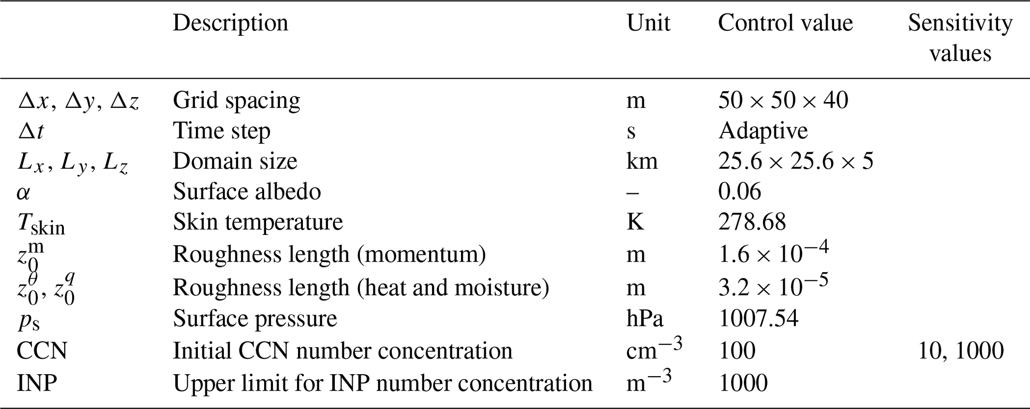
The observed statistical distribution of aerosol concentration as shown in Fig. 4 informs the initial CCN profile adopted in the control experiment, chosen here to be constant with height at 100 cm−3. This choice is motivated by the following arguments. Firstly, it is safe to assume that only a fraction of the observed aerosol can act as CCN, here assumed to be approximately 50 %–90 %. Secondly, CCN are treated prognostically in the model and can evolve freely during the simulations, and no external sources of CCN are considered for simplicity. With the convection and clouds gradually removing aerosol below the inversion (Bigg and Leck, 2001), a choice of 100 cm−3 should after some time result in a vertical structure resembling the observed one as shown in Fig. 4, with concentrations below the clouds being about half of the values above. The sensitivity to CCN is tested by means of two additional experiments. One experiment adopts 10 cm−3, representing pristine air as often found in the high Arctic. The other adopts 1000 cm−3, representing polluted air from continental origins. Both extremes are frequently observed in Arctic air masses (Bigg et al., 1996; Stohl et al., 2006; Garrett et al., 2010).
The initial cloud droplet number concentration in supersaturated areas is set accordingly: the initial mean droplet size must be higher than the advised threshold g (Seifert and Beheng, 2006a), and at most of the initial CCN number concentration is activated. The motivation for this initial concentration is straightforward: the simulation can start with neither too large nor too small droplets and spins up without encountering a lack of CCN. The number concentration of INPs is assumed time constant and prescribed at 1000 m−3, therein following Reisner et al. (1998) and M. Hartmann et al. (2019).
The main goal of the evaluation of the control experiment is to test to what extent the bulk characteristics of the observed boundary layer and clouds are reproduced. This approach is in line with previous LES studies of Arctic mixed-phase clouds (e.g., Ovchinnikov et al., 2014; Stevens et al., 2018; Neggers et al., 2019). Bulk statistics here include the mean vertical structure as well as various heights, such as the cloud boundaries and inversion. The availability of in situ cloud and turbulence measurements during RF20 allows us to go one step further and also evaluate profiles of liquid and frozen hydrometeor mass as well as turbulent (co)variances.
4.1 Time evolution
Figure 5a and b document the time development of the domain-averaged cloud structure and phase during the control simulation of the composite RF20 case. After a spinup period of about 12 h the boundary layer more or less equilibrates, staying close to this state for the remainder of the simulation. The cloud layer is in the mixed phase, with liquid cloud coexisting with ice cloud. Both specific mass concentrations reach a maximum immediately below the inversion. A weak diurnal cycle in cloud mass, cloud thickness, and inversion height can be distinguished, superimposed on the long-term equilibrium (better visible in time series data shown later in Fig. 13). Such diurnal signals are well known from warm marine stratocumulus and are driven by daytime absorption of shortwave radiation alternating with nighttime cloud top cooling (Rozendaal et al., 1995; Wood et al., 2002; Duynkerke et al., 2004). The presence of this signal here indicates that in early June the solar radiation is already strong enough at these latitudes to drive a boundary layer response.
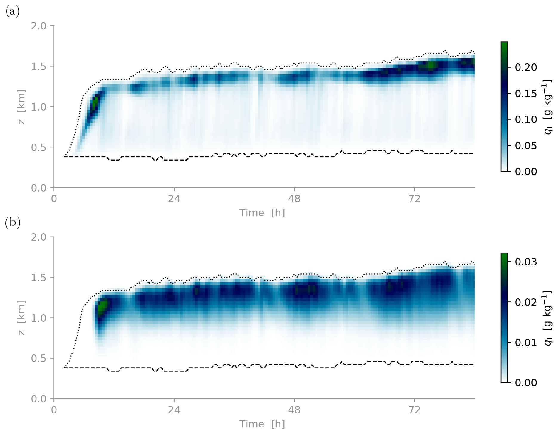
Figure 5Time–height contour plots of domain-averaged variables during the control experiment. Specific mass of (a) cloud liquid water ql and (b) cloud ice water qi. The averaging time is 30 min. The dashed and dotted lines reflect the lowest base and highest top of liquid clouds in the domain, respectively.
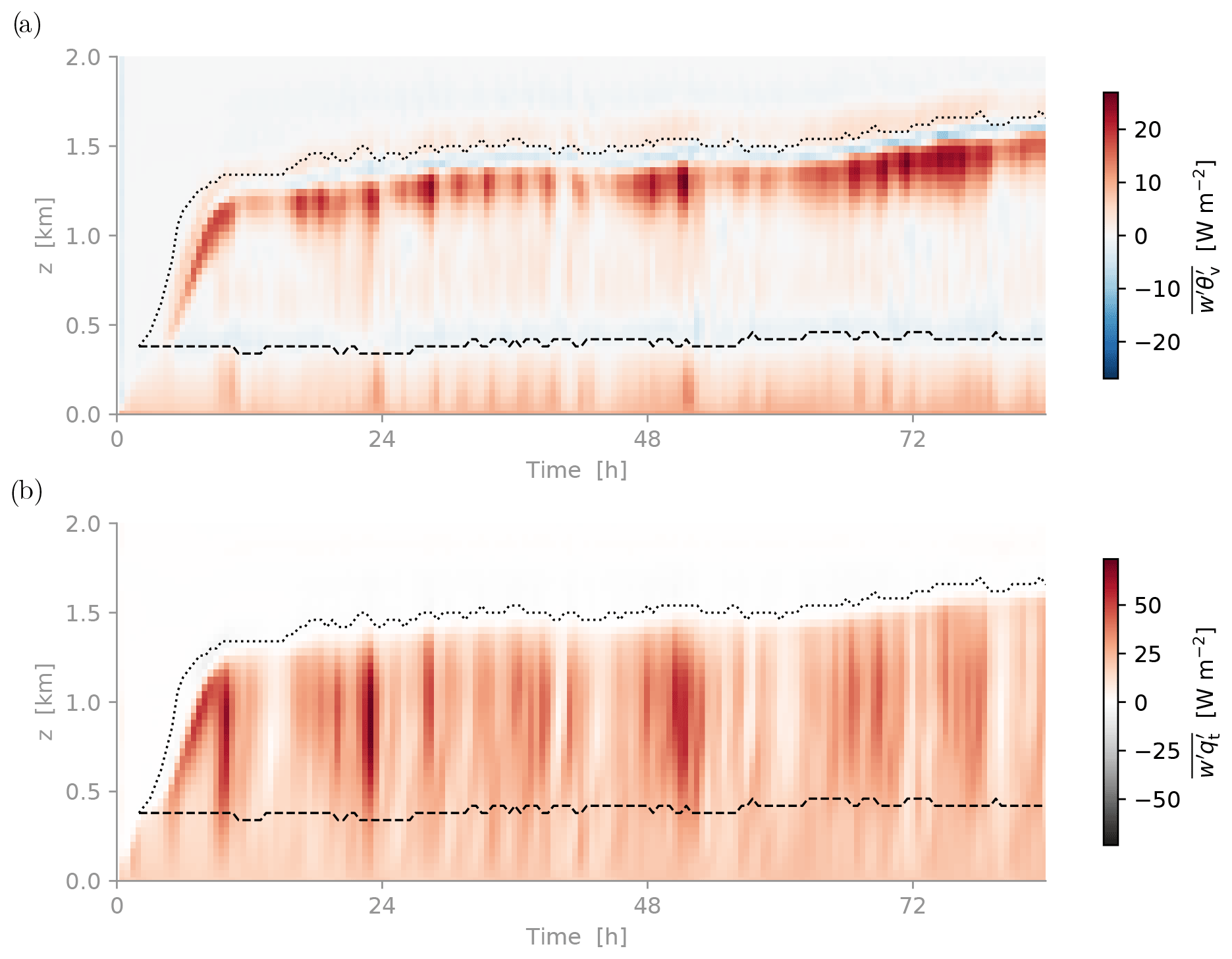
Figure 6a and b show the total (resolved + subgrid) fluxes of virtual potential temperature and total specific humidity. Significant boundary-layer-deep transport is present, reflecting a high degree of coupling between the cloud layer and the surface. This aspect makes this case distinctly different from turbulent mixed-phase clouds over homogeneous sea ice, which are often fully decoupled (e.g., Solomon et al., 2014). The evolution of the humidity flux shows that it takes about 12 h for the surface-driven turbulence to properly spin up after initialization. Once this has occurred the transport is continuous, with the local minimum in the θv flux near the liquid cloud base indicating the presence of a shallow transition layer (see Fig. 6a). Such stable layers with CIN (convective inhibition) are a well-known feature of cumulus-capped boundary layers (Albrecht et al., 1979) and decoupled stratocumulus (Nicholls, 1984). The transport intensity is intermittent at times, which could reflect the impact of subsampling of convective events due to a still limited domain size.
4.2 Vertical structure
The simulated vertical profiles of three state variables at three time points are compared to the dropsonde sounding data in Fig. 7. In general the simulated profiles agree well with the observations concerning the vertical structure of the boundary layer, with a relatively well-mixed layer up to about 500 m capped by a cloud layer that features a conditionally unstable thermodynamic lapse rate. This cloud layer with high relative humidity extends up to about 1.4 km. The inversion layer of a few hundred meters deep is also reproduced well, featuring a θv jump of about +3 K and a negligible qv jump. During the 48 h simulation this vertical structure does not change much, with the boundary layer only deepening by about ∼150 m.
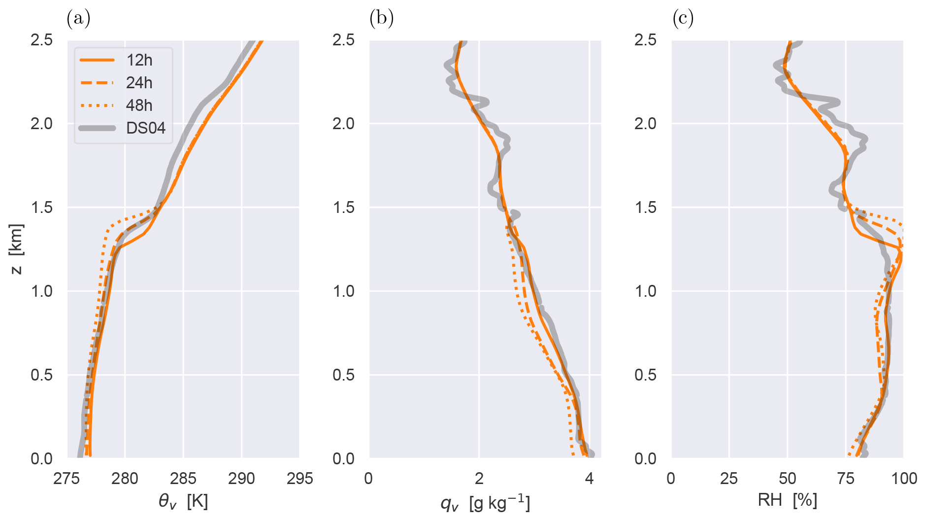
Figure 7Domain-averaged vertical profiles during the control experiment. (a) Virtual potential temperature θv. (b) Water vapor specific humidity qv. (c) Relative humidity RH. The DS04 dropsonde sounding is shown in grey. Three subsequent time points are shown.
Figure 8 shows domain-averaged vertical profiles of all five hydrometeor species of the DALES microphysics scheme at t=24 h, grouped as suspended and falling species. This time point was chosen based on the good agreement of the inversion height with the observations (see Fig. 7). Cloud liquid water ql has a distinct mode near the inversion but still has significant values below, reflecting the presence of rising convective updrafts. Cloud ice qi also peaks near the inversion but disappears a few hundred meters above the liquid cloud base. These amplitudes in ql and qi compare well to previous studies of convective mixed-phase clouds over open water in the Arctic (Klein et al., 2009; Morrison et al., 2009). Snow qs and graupel qg masses peak in the middle of the cloud layer and turn into rain qr below the freezing-level height at z∼400 m. Significant precipitation mass is lost on the way down due to sublimation and evaporation (at the altitudes below the freezing level). Rain shafts reaching the surface are consistent with the observations; they are visible in the radar measurements shown in Fig. 2.
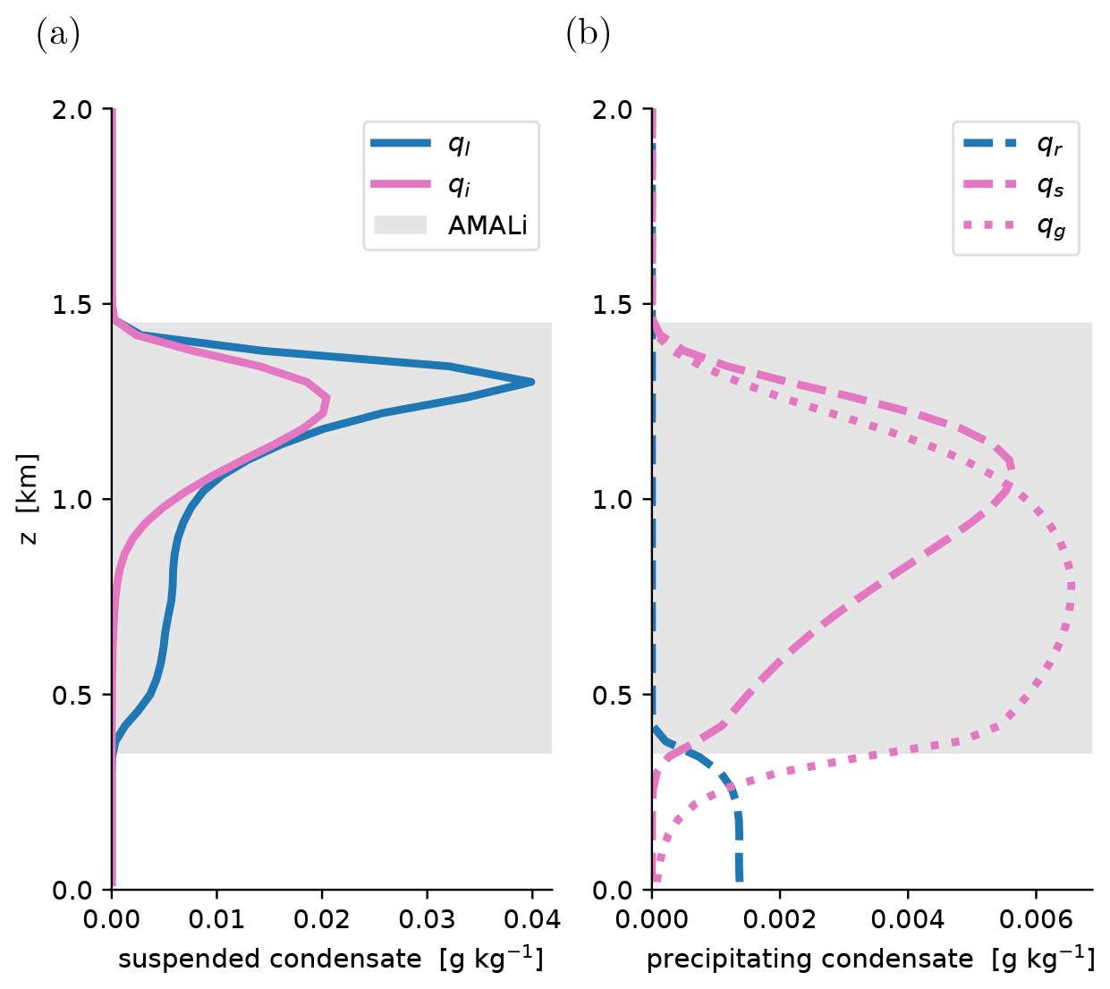
Figure 8The specific masses of all five hydrometeor species in the control simulation at t=24 h. (a) Suspended species, including liquid water ql and ice water qi. (b) Precipitating species, including rain qr, snow qs, and graupel qg. Liquid species are shown in blue; frozen species are shown in pink. The vertical range of AMALi cloud top heights sampled within the target domain as shown in Fig. 2 is shaded grey.
4.3 Cloud boundaries and hydrometeors
Figure 8 also indicates the range of cloud top heights as sampled by the AMALi instrument on board P5 (data shown in Fig. 2). This range only reflects AMALi data sampled within the modeling domain, which was visited three times in short succession. Because the cloud deck was not homogeneous and contained numerous gaps, the data include sufficient hits at lower heights to yield a representative estimate of cloud layer depth. The model liquid water fits well between the AMALi cloud layer boundaries in the control experiment at this time point (t=24 h), consistent with the good agreement on inversion height as detected by the dropsonde.
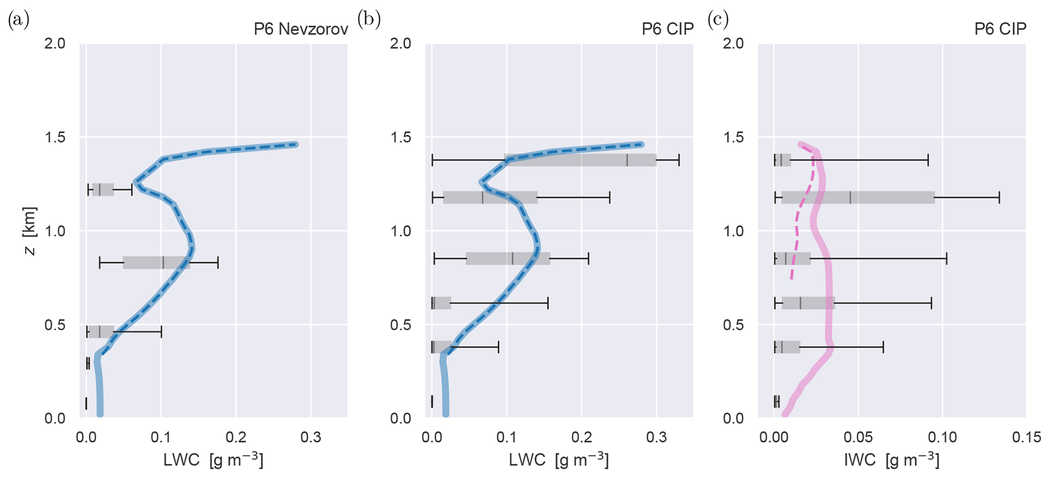
Figure 9Simulated and observed hydrometeor masses. Panels (a) and (b) show liquid water content (LWC) sampled by the Nevzorov and CIP probes, respectively, while panel (c) shows the ice water content (IWC) measured by the CIP probe. Only samples during the southern racetrack segment of RF20 are included. The hourly mean LES results at t=24 h are shown in color and represent conditional averages over the area fraction covered by the associated hydrometeors. The thick colored line represents the sum of all liquid-phase hydrometeors (blue, ql+qr) and ice-phase hydrometeors (pink, ) in the model. The thin dashed line represents only the suspended species (ql and qi, respectively). The grey box–whisker plots represent the P6 measurements in the racetrack section, with the 5th–95th percentile range (black line) and the interquartile range (grey box) indicated. The Nevzorov data are analyzed on five separate level flight legs, while the CIP data are vertically gridded at 250 m spacing.
Figure 9 evaluates the hydrometeor mass in the LES against the in-cloud measurements by the Nevzorov and CIP probes on board P6. The hourly mean LES results at t=24 h are shown in color, while the observational data are shown as box–whisker plots. A complication with hydrometeor evaluations of this kind is that their definition in the microphysics scheme might not necessarily match that of the observation system. For example, for ice hydrometeors it is hard to separate between suspended (cloud) and precipitating particles. To avoid such problems the comparison is made as straightforward as possible, by only making comparisons based on phase. This means that in each panel the simulated and observed values include all hydrometeor species in the phase of interest. For the LES this means for liquid and for ice (shown as thick lines in Fig. 9). For the CIP probe the full size distribution of ice particles can thus be included in the data. Note that the LES microphysics scheme does include secondary ice production, allowing for the formation of large and heavy ice hydrometeors in the simulation (Sullivan et al., 2017; Georgakaki et al., 2022). For reference, the mass of only the suspended model hydrometeors is also indicated (dashed line).
Figure 9a and b compares the liquid-phase hydrometeor mass of the LES to the Nevzorov and CIP measurements, respectively. Note that the vertical gridding of the data are slightly different for each instruments; for the Nevzorov probe the box–whisker plots represent data on five separate straight flight legs, while for the CIP probe a vertical gridding of 250 m is used. The model data are conditionally averaged over the area where the hydrometeors occur; this way, the contribution by hydrometeor-free air to the average is excluded, and the comparison with the in-cloud observational data are fair. While slight differences exist in liquid water content (LWC) between the two probes, in general they agree on the magnitude and vertical structure. The observed mean LWC peaks in the middle of the cloud layer at ∼800 m height and again near the inversion at ∼1400 m. The LES always sits within the observed 5th–95th percentile range in the cloud layer and is reasonably close to the interquartile range. It also reproduces the vertical structure, which is encouraging. Some LWC is detected below the AMALi cloud base (∼400 m), which is probably rain. Including rain qr in the LES data shows that the model is consistent with this feature.
Figure 9c then evaluates the mass of all frozen hydrometeors against the CIP data. The data show that large spread exists but that on average the IWC mass is considerably smaller in magnitude compared to the observed LWC. Also note that some ice is observed below the cloud base. The model is again situated within the 5th–95th percentiles. This time, a considerable difference exists between the suspended and falling hydrometeors in the LES; suspended cloud ice qi is only present near the inversion (dashed line), while snow qs and graupel qg contribute most of the frozen hydrometeor mass at lower heights. Including those falling species is needed to explain the observations at lower heights.
We conclude from this analysis that the model is representative of the observed clouds, both for the liquid and ice phase. It should be noted in this respect that the observed sample size of hydrometeors is still limited; only relatively few clouds were sampled by P6 on the racetrack, also during a limited period. This introduces some uncertainty, preventing us from drawing any conclusions beyond the bulk (mean) state. Any higher-order evaluations, for example concerning spatial variability or particle size distributions, require much more substantial datasets and therefore go beyond the scope of this study.
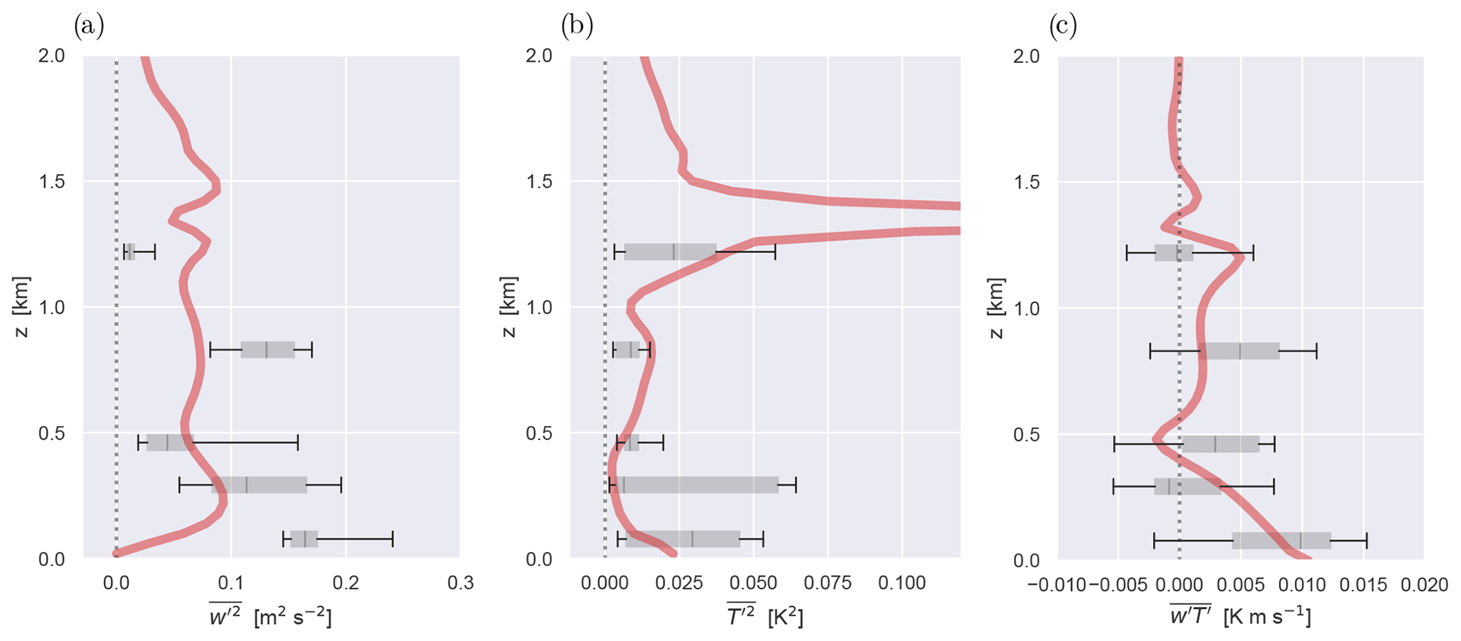
Figure 10Simulated and observed turbulent (co)variances, including (a) the vertical velocity variance , (b) the temperature variance , and (c) the associated temperature flux . Similar to Fig. 9 the box–whisker plots again indicate P6 measurements, this time showing nose boom data during the five level flight sections on the southern racetrack. The mean LES profile at t=24 h is shown in red.
4.4 Turbulence
The measurements at 100 Hz of temperature and vertical velocity made by the sensors in the P6 nose boom during RF20 (M. Hartmann et al., 2019) allow for calculating variances of both variables, as well as the turbulent heat flux. On the RF20 southern racetrack five segments at constant heights within the lowest 2 km were included for this purpose, adopting the well-known method as explored in previous classic studies (Nicholls and Lemone, 1980). Although this area is located slightly to the west of the DS04 target area, the near-surface turbulence is expected to be similar in both. A running average of 10 min is calculated, based on which time series of the (co)variances can be estimated.
Figure 10 shows the distribution of (co)variances on each of the five level flight legs. Observational data are again shown in the box–whisker style, similar to Fig. 9. LES data again reflect hourly averages around t=24 h. Below the cloud base (∼450 m) the LES profiles exhibit some well-known features of turbulent mixed layers, including a convex structure, a concave structure, and a linear decrease in the heat flux towards slightly negative values near the layer top. The latter is consistent with the local minimum in the buoyancy flux seen in Fig. 5d. These vertical structures are not clearly visible in the observations; however, a large spread exists at each flight leg, and the model is almost always situated within the observed 5th–95th percentile range. The exception is at the lowest and highest flight legs, which we speculate could be caused by the strong variability in w in the close vicinity of convective cells. In the middle of the cloud layer (∼900 m) the model data show a second maximum, reflecting the impact of latent heat release on turbulence. Near the inversion the temperature variance peaks as expected, due to the close vicinity of a strong temperature gradient. This feature in the model is also supported by the measurements.
The general outcome of this evaluation is that the LES turbulence profiles are mostly situated within the observed 5th–95th percentile range, with a few small exceptions. The data suggest that the agreement is best for the temperature variance and the vertical heat flux, with the LES sitting reasonably close to the interquartile range. This supports the conclusion that the amplitude and vertical structure of both the intensity and transport of the convection and turbulence in this case are reasonably well captured by the model.
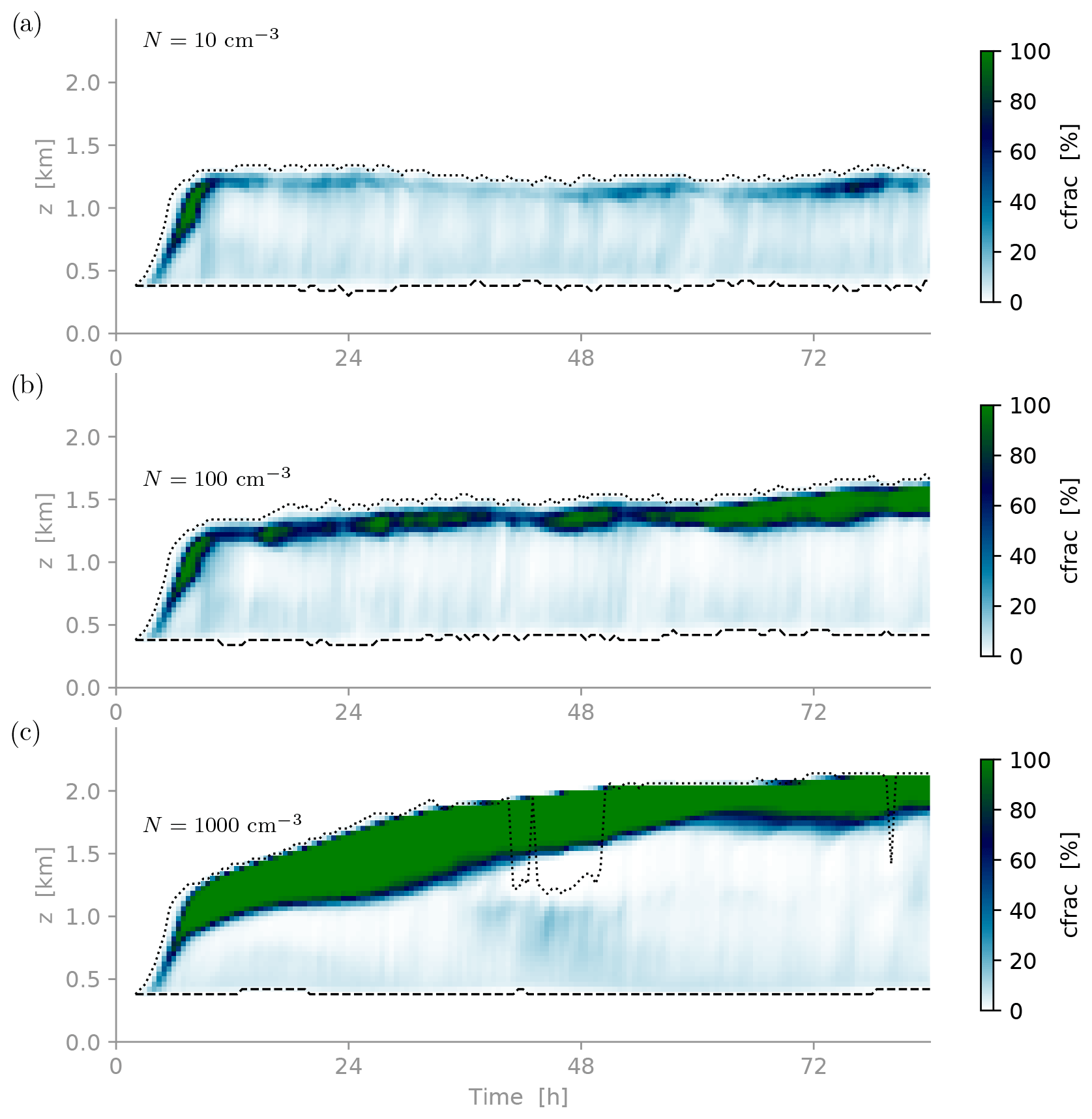
Figure 11Time–height contour plots of liquid cloud fraction (cfrac) during the three CCN sensitivity experiments. (a) Pristine high-Arctic conditions (N=10 cm−3). (b) Control conditions observed during ACLOUD RF20 (N=100 cm−3). (c) Polluted continental conditions (N=1000 cm−3). Liquid cloud fraction is calculated at each vertical layer as the fraction of grid points where the cloud liquid water content is above the threshold (set to 0.01 g m−2 for cloud liquid water).
With a satisfactory agreement between the control run and the measurements established, the next step is to assess the sensitivity of the results to the aerosol levels in the simulated air mass. A few recent LES intercomparison studies on Arctic mixed-phase clouds have investigated this dependence. Stevens et al. (2018) investigated three LES codes for a tenuous mixed-phase stratocumulus case observed over sea ice, reporting that the lack of CCN can seriously limit the liquid water path (LWP). Higher CCN concentration levels in a marine cold-air outbreak case were studied by de Roode et al. (2019), finding that this leads to increased LWP. The RF20 case studied here is similar to the CAO case but also differs considerably, in particular in the much weaker convection and the stagnancy of the air mass. Our goal is to investigate and understand the impact of CCN also for these conditions. Specific focus lies on the efficiency of radiatively driven entrainment, the role played by the ice phase, and the impacts on the energy budgets of the boundary layer and the surface. A much wider CCN concentration range is covered compared to the previous LES studies. This allows for interpretation of the consequences of CCN impacts for air mass transformations and air–ocean interactions in this region of the Arctic.
5.1 CCN
The two additional experiments with N={10, 1000} cm−3 are designed to reflect observed extreme CCN conditions in the area of interest. The lower value represents pristine conditions typical of the high Arctic, while the higher value represents polluted continental conditions as sometimes encountered in warm and moist air intrusions from the mid-latitudes (Bigg et al., 1996). The N=100 cm−3 value of the control experiment is based on in situ P6 measurements in the air mass during ACLOUD RF20. Accordingly, together these values span a realistic CCN range.
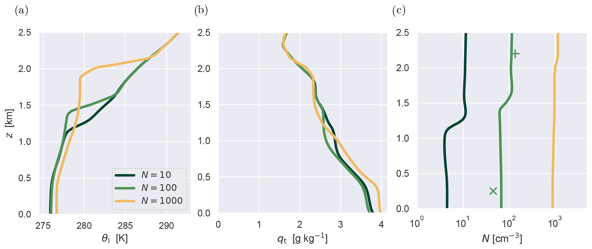
Figure 12Profiles of (a) liquid water potential temperature θl, (b) total water specific humidity qt, and (c) the CCN concentration N for the three CCN experiments. Data are time-averaged over the last 48 h. Colors represent the initial CCN concentration (cm−3). The modes of the measured concentrations below (×) and above (+) the cloud layer (shown in Fig. 4) are also indicated, for reference.
Figure 11 shows time–height contour plots of the area fraction of liquid cloud water in three CCN sensitivity runs. The depth of the boundary layer shows a strong response, deepening from 1.2 km to above 2 km for the continental setup. The capping liquid cloud layer situated immediately below the inversion also thickens considerably. Note that only the control N=100 cm−3 experiment is close to the observed cloud top height. During the first 48 h of the continental experiment the deepening is so aggressive that the stratiform cloud layer shows signs of decoupling from the surface-driven convection below, probably because of large top entrainment rates. This decoupling is indicated by a steepening of the virtual potential profile and a gap in the cloud fraction forming above 1100 m, nearly separating the cloud layer into two distinct layers in Fig. 5c (32–48 h interval).
Figure 12 documents the impact of CCN on the thermodynamic structure and depth of the convective boundary layer. For larger N values, the convective mixing reaches deeper into the air mass in which it is embedded, lifting the thermal inversion. An important side effect is that it also makes the thermal inversion stronger, as expressed by the increased jump in θl across the inversion layer. The boundary layer in the continental CCN experiment has also warmed and moistened significantly compared to the other two runs. The vertical structure of N reveals its time evolution, with concentrations below the inversion gradually decreasing due to removal by precipitation. During the simulated period this decrease is only limited, with CCN levels in the convective layer still retaining substantial values. This vertical structure in the model is also consistent with the P6 observations, with the N=100 cm−3 experiment sitting closest to the observed amplitude above and below the cloud layer.
Figure 13 compares the evolutions of vertically integrated or projected cloud properties during the three CCN sensitivity runs. The liquid cloud cover al is in the model defined as the fraction of the domain where the vertically integrated cloud liquid water exceeds the minimum threshold of 0.01 g m−2. The liquid cloud cover goes from about four octas for pristine conditions to persistent full cover for continental conditions. The liquid water path (LWP) also increases with CCN, temporarily reaching very high levels during the spinup of the high-CCN run, before settling at a lower value. The ice water path (IWP) increases more or less monotonically. None of the experiments have fully equilibrated at the end of the simulation, with the N=1000 cm−3 experiment seeing the largest drift. A weak diurnal cycle is visible in all three variables. Interestingly, before the appearance of cloud ice the three cases evolve almost identically; it is only afterwards that significant differences develop. Although the ice initiation is not dependent on the cloud droplet size, the large droplets nevertheless contribute to the development of the ice phase. The reasons are the following: firstly, larger cloud droplets are more likely to undergo heterogeneous freezing; secondly, larger cloud droplets are more likely to collide with ice particles and freeze. The ice particles then join more mass, leading to increased fall velocity and thus further collisions. Additionally, when the collision occurs, the freezing large droplet produces more splinters (Hallett and Mossop, 1974). On the other hand in the simulation with high CCN concentrations, the cloud water is distributed over higher-number cloud droplets, leading to weaker riming tendencies and thus slower development of the ice phase (see Fig. 15b). This suggests that ice formation plays a key role in how CCN impacts the boundary layer clouds.
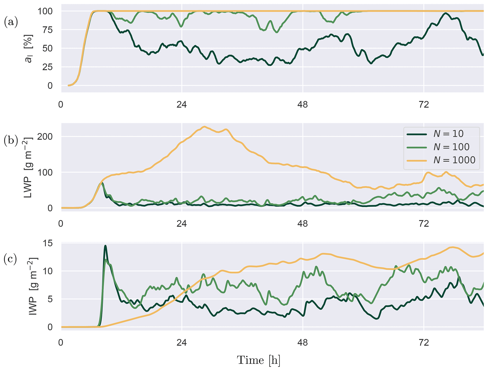
Figure 13Time series of domain-averaged microphysics properties during the three CCN sensitivity experiments. (a) Liquid cloud cover al. (b) Cloud liquid water path LWP. (c) Cloud ice water path IWP.
Figure 14 then summarizes the impact of CCN on a selection of bulk properties of the convective boundary layer, presented as a bar plot of time averages that cover the last 48 h of the simulation. This is done to effectively remove any diurnal cycle in these signals. The changes shown in the top four panels indicate that the response of the boundary layer clouds to a CCN increase as detected in this case is in principle similar in sign compared to the cold-air outbreak case studied by de Roode et al. (2019). Boundary layer depth zt is here calculated as the height at which is maximum. Depth zt increases along with the liquid and frozen cloud amount LWP and IWP, while the surface precipitation P decreases, consistent with the second cloud–aerosol indirect effect.
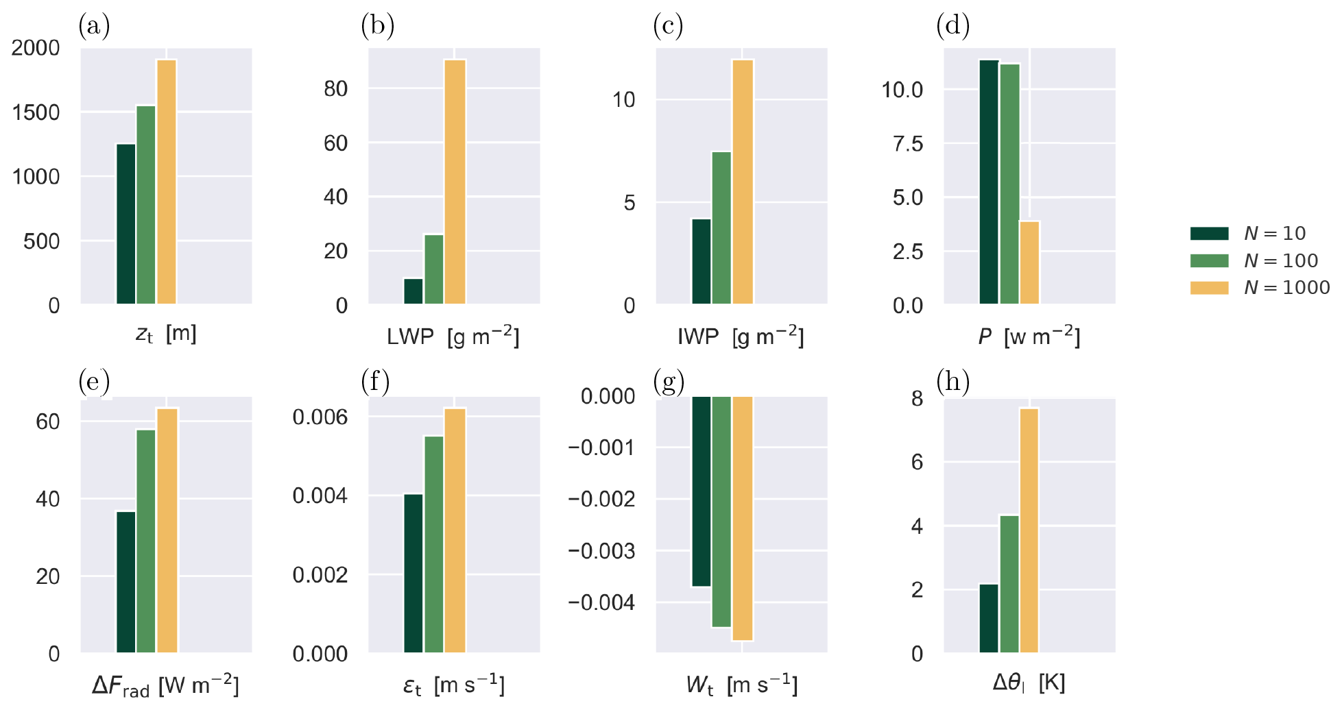
Figure 14Bar plots of diurnally averaged bulk properties of the convective boundary layer, for all three CCN experiments as shown in Fig. 13. (a) Boundary layer depth zt. (b) LWP. (c) IWP. (d) Surface precipitation rate P. (e) Net longwave radiative flux divergence across the liquid cloud layer ΔFrad. (f) Top entrainment rate ϵt. (g) Large-scale vertical velocity at boundary layer top Wt. (h) Jump in liquid water potential temperature Δθl across the inversion. The time averaging covers the last 48 h of the simulations.
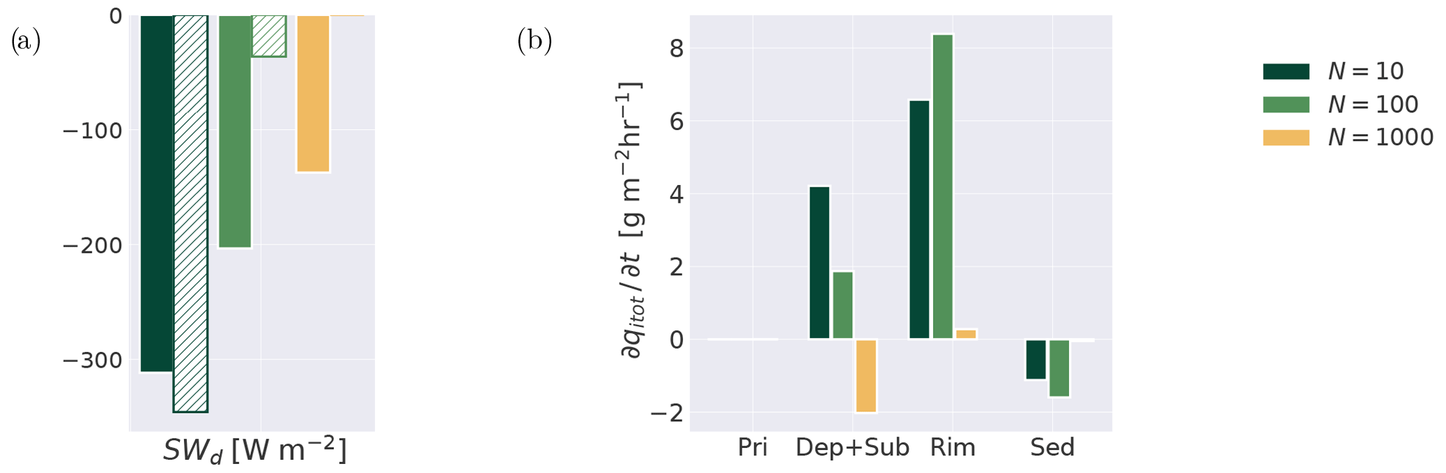
Figure 15Bar plots of the effects of cloud processes. (a) The comparison of the shortwave downward flux estimated from the Twomey formula (shown as bars with the pattern) and the shortwave downward flux from the from the simulation output (shown as full colored bars); (b) vertically integrated tendencies in (total) ice water mass budget within the cloud layer: primary ice nucleation and freezing of cloud droplets (Pri, significantly smaller than other tendencies), the combined effect of deposition and sublimation (Dep + Sub), riming of cloud droplets (Rim), and sedimentation (Sed). The time averaging covers the last 48 h of the simulations.
Another indirect effect of the aerosols in the Arctic is the change in the shortwave downward radiative flux due to changes in the optical properties of the clouds (Markowicz et al., 2021; Im et al., 2021). We estimate the Twomey effect using the simple formula (Twomey, 1977) for the optical depth τ:
where N is the number concentration of the cloud droplet per unit of volume, is the mean radius of cloud droplets, and h is the depth of the cloud. Based on the τ calculated from the mean values over the cloud layer, we estimate the transmitted shortwave downward radiative flux and compare it with the shortwave downward flux from the simulation output (see Fig. 15a). There is a reasonably good agreement for the pristine conditions (N=10 cm−3) but a significant underestimation for the control case. Finally for the continental case, the estimated Twomey effect differs from the simulation by more than an order of magnitude. However, this outcome is not surprising in the Arctic (Yang and Liu, 2022) given the non-uniform structure of the mixed-phase clouds with regions of lower cloud fraction in the middle and lower portion of the cloud layer (Fig. 11c).
The lower four panels of Fig. 14 provide more insight into the impact of CCN on the turbulent mixing at the inversion. As one expects, the net longwave radiative flux divergence across the liquid cloud layer ΔFrad increases with LWP. It seems to saturate towards very large CCN, reflecting shifts in both cloud top cooling and cloud base warming (Stevens et al., 2005). As is well known, the cloud top cooling generates turbulence, which in turn drives entrainment of overlying dry and warm air into the boundary layer. The associated top entrainment rate ϵt at zt is here calculated as the residual from the boundary layer mass budget:
with Wt being the large-scale vertical velocity at zt. Figure 14f confirms that the entrainment rate increases in a similar tread as ΔFrad. Note that the prescribed subsidence increases with height in this case (see Fig. A1). As a result, the CCN-richer boundary layer also equilibrates at a higher zt. The slight inequality of ϵt and −Wt again reflects that the equilibration has not yet completed at the end of the simulated period.
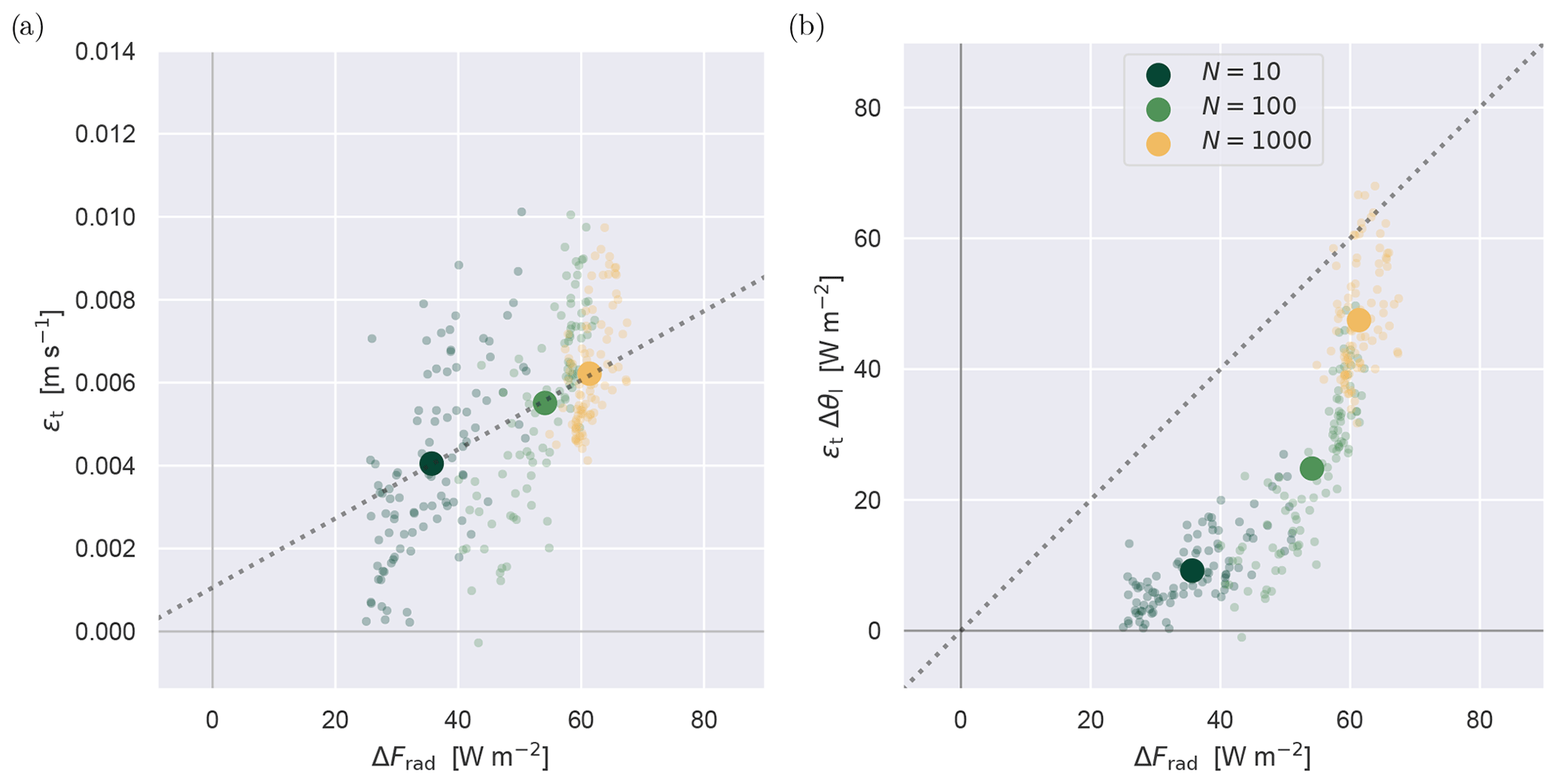
Figure 16Scatter plots of terms in the radiative entrainment efficiency α, as defined by Eq. (3). The net longwave flux difference across the cloud layer ΔFrad is plotted against (a) the top entrainment rate ϵt and (b) the entrainment flux ϵtΔθl in energy units. Diagnostics at 2 h−1 frequency are shown as small semi-transparent dots, while the 48 h mean is shown as an opaque big dot. In panel (a) the dotted line represents the linear fit through the means, while in panel (b) it represents the line at which α=1.
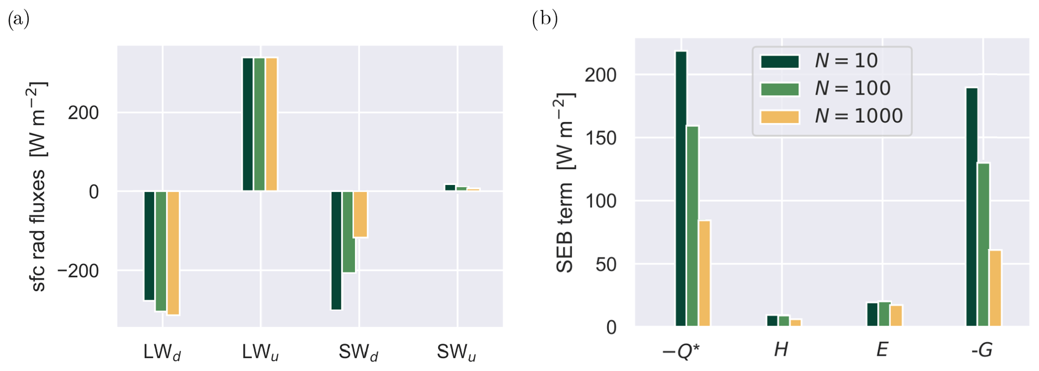
Figure 17Same as Fig. 14 but now showing various surface (sfc) energy fluxes. (a) All four components of the net radiative energy flux Q*, separated between longwave (LW) and shortwave (SW) bands as well as upward (u) and downward (d) directions. (b) All terms in the surface energy budget (SEB), including net downward radiation , upward sensible heat H, upward latent heat E, and downward ground heat −G. The values are horizontally averaged over the whole surface; the time averaging then covers the last 48 h of the simulations.
Entrainment warming and cloud top cooling counteract each other in the heat budget of the boundary layer. Which one wins is expressed by the radiative entrainment efficiency α, defined by Stevens et al. (2005) as
where Δθl is the jump in liquid water potential temperature across the thermal inversion, here defined as the layer between the first maximum and minimum in the second derivative of below and above zt, respectively. Figure 16 shows scatter plots of various components in Eq. (3). Although considerable scatter exists at small timescales, a well-defined linear relation exists between the time-averaged ϵt and ΔFrad, confirming that cloud top cooling is driving the entrainment. Figure 16b then shows that cloud top cooling is almost always stronger than the entrainment heating, representing entrainment inefficiency (α<1). However, the efficiency improves towards higher CCN concentrations, approaching α=1 for continental conditions. At this point, entrainment warming is almost fully compensating the cloud top cooling. Comparing both panels indicates that this has to be caused by a non-linear increase in Δθl, a measure of thermal inversion strength (shown in Fig. 14h). The strengthening can be explained as a consequence of a deep mixed layer growing into a weakly stable overlying layer. Apparently, the boundary layer responds to a CCN concentration increase by both strengthening the inversion and boosting the warming efficiency of radiatively driven entrainment. This is an interesting outcome in the context of Arctic amplification, given that both processes play a role in the lapse rate feedback.
The impact on the surface radiative fluxes is considered in Fig. 17a. While the downward longwave flux sees a relatively small increase, the downward shortwave flux strongly reduces by about 200 W m−2, reflecting that most of the solar radiation is now reflected at the liquid cloud top. Although this is less that what would be expected in the Twomey effect (as shown in Fig. 15a), it is nevertheless a significant difference. As a result, the downward net radiative flux at the surface (shown in Fig. 17b) reduces by about 130 W m−2. This energy flux is the main driver of the surface energy budget (SEB), which, following Stull (1988), can be defined as
where H is the upward sensible heat flux, E is the upward latent heat flux, and −G is the downward heat flux into the ocean. As is often the case with the SEB over oceans for daytime weakly unstable conditions, H and E are typically much smaller than the net radiation and ocean heat flux. Moving from pristine to continental CCN values reduces both H and E by a small amount. But the reduction in both and −G is much larger, with the one more or less compensating the other. In other words, the flow of energy through the SEB is diminished, resulting in a reduced energy flux into the ocean.
With the main results thus described in detail, we now proceed with a more general discussion of their implications, in various contexts.
6.1 Constraining LES with observations in the Arctic
The results show that the control setup yields a simulation that equilibrates close to the observed thermodynamic, turbulent, and cloudy state of the marine boundary layer as probed during ACLOUD RF20. Part of this control setup is the independently sampled CCN value of N=100 cm−3 by P6 during RF20 (see Fig. 4). Given the large sensitivity of the results to CCN as found in this study, the good agreement of the control experiment with the RF20 data is not trivial. It implies that the availability of such in situ aerosol measurements is crucial for the successful configuration of subsequent LES experiments that are to realistically reflect observed conditions. This finding is thus a recommendation for future field campaigns in the Arctic.
6.2 Air mass transformation
Figure 12 further illustrates the profound impact of CCN on the boundary layer structure and depth in this cloud regime over open water. These findings indicate that CCN can act as a catalyst for the convective mixing into the air mass. For higher CCN concentrations, the convective mixing reaches deeper into the air mass in which it is embedded, lifting the thermal inversion and making it stronger. In particular radiatively driven turbulent entrainment becomes more efficient compared to surface-driven convection. This CCN impact thus plays a role in how air masses transform as they travel over open water near the sea ice edge. In case it travels onward into the high Arctic, its properties at lower levels will be more diluted as a result, affecting its net impact on the Arctic climate system (Pithan et al., 2018). Numerical simulations covering a much larger domain in the Arctic but still resolving entrainment to a reasonable degree, as well accounting for the impact of CCN on its efficiency, could provide further insight.
6.3 Climate impacts
It is interesting to interpret the impact of CCN on the entrainment efficiency as found in this study in the context of Arctic amplification, in particular the lapse rate feedback (LRF). This would mainly work through the low-level heat budget. As defined by Eq. (3), the entrainment efficiency reflects the ratio of two terms in this budget, namely entrainment warming and longwave radiative cooling. But the full heat budget contains a few more terms, which might also play a role. To find out, we now consider the budget for the layer of air below the base of the boundary layer thermal inversion, here taken as the base height of the layer over which the jump Δθl was calculated (shown in Fig. 14h). The vertically integrated bulk budget of sensible heat can then be written as
where h is layer depth. A dot indicates a tendency, and the brackets indicate a vertical average over depth h. A distinction is made between the contributions by physical processes and large-scale forcings, indicated by subscripts “p” and “f”, respectively. The physics term can be further expanded as
where ΔFLW and ΔFSW represent the difference in longwave and shortwave flux across the layer and Fϵ stands for the entrainment flux at the layer top. Note that by considering only the layer below the base of the thermal inversion, the reduction in h (or loss of mass) due to subsidence within the inversion layer is excluded.
Figure 18 shows all budget terms as averaged over the last 48 h. By convention, a term is positive when it contributes heat to the layer. Longwave cooling ΔFLW is always the main sink, counteracted by surface fluxes H and P, entrainment warming Fϵ, and shortwave absorption ΔFSW. These physics approximately balance the sink term due to layer-internal large-scale forcing (including prescribed horizontal advection and subsidence). Adding CCN significantly shifts this balance, with surface fluxes becoming less important and radiative and entrainment terms becoming more dominant. In other words, the turbulence shifts from surface driven to radiatively driven. The entrainment flux contributes most to the enhanced net heating tendency, which implies that the boosted entrainment efficiency as previously discussed in Sect. 5.1 drives the net response of the boundary layer energy budget.
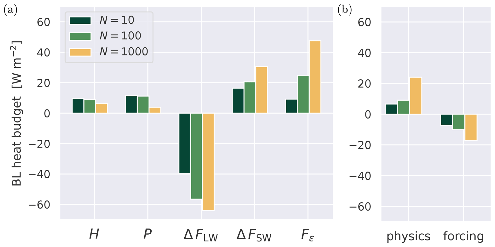
Figure 18Analysis of the bulk (BL) heat budget of the boundary layer below the base of the capping inversion. (a) Bar plot of all physics terms in the sensible heat budget, plotted as energy fluxes. (b) The net contribution by all physics terms as shown in panel (a) and the large-scale forcing .
What these results imply is that the impact of CCN on the low-level energy budget through the entrainment efficiency is substantial and can not be ignored for understanding the LRF. In this respect it is worthwhile to remember that our simulations reflect clouds over open water. Recent studies have emphasized the importance of considering the partitioning between marine and ice-covered areas in understanding the LRF (Jenkins and Dai, 2021). In newly formed open-water areas where sea ice has disappeared, one expects the lower-level stability to decrease. However, our results suggest that this does not automatically imply a weakened inversion, in the case that the melt is accompanied by a simultaneous increase in CCN (Browse et al., 2014).
6.4 Atmosphere–ocean interactions
We find that for high CCN levels in the air mass the SEB is greatly reduced, featuring a much smaller flux of energy into the ocean. This has a cooling effect on the oceanic mixed layer, which in the long term might percolate to greater depths where the main ocean circulation takes place. Note that in our simulations the ocean skin temperature was prescribed such that G is calculated as a residual of the SEB. In other words, the changes in net radiation do not feed back into the sensible and latent heat fluxes, which only depend on the lower-atmospheric state. Additional LES runs including a simple but interactive oceanic bulk mixed layer would allow this two-way air–ocean interaction to take place. This could give insight into the typical timescale of the adjustment process, the sign and magnitude of the air–ocean feedback, and the amount of energy lost to deeper parts of the oceanic mixed layer. Such simulations are considered a future research effort. Another factor to be considered when interpreting the impact of the large radiative flux differences on the Arctic climate system is that the actual frequency of occurrence of this cloud regime in the area of interest is not yet considered in this study.
6.5 Further sensitivities
Some aspects of the experimental design can affect the behavior of the simulated turbulence and clouds. These include the size of the turbulent domain, the spatial and temporal discretization, and the way the larger-scale forcing is configured. For example, one could adopt heterogeneous boundary forcing in a nested setup, which allows for representing advection of mesoscale features into the domain that are now ignored. While this might aid realism, it would make the simulation more complex and perhaps harder to interpret in terms of the response of convection to CCN. Another key model component is the microphysics scheme, for which one also expects sensitivity. In a follow-up study the authors explore some of these potential sensitivities for this ACLOUD case.
Observational data collected by the P5 and P6 polar research aircraft in a relatively stagnant air mass over the Fram Strait during ACLOUD RF20 were used to test the skill of LES in reproducing observed key characteristics of mixed-phase convection over open water near the sea ice edge. A unique aspect of this campaign is the availability of in situ aerosol measurements directly above and below the cloud deck. These allow for realistic initialization of CCN in the LES and create opportunities for gaining insight into how aerosol content in the air mass affects the mixed-phase convection. Our main conclusions can be summarized as follows:
-
The observed thermodynamic, kinematic, turbulent, and cloud structure are well reproduced by the model when initialized with the observed CCN concentration.
-
Changing the CCN concentration in the air mass from pristine to continental values substantially alters the cloud amount, the boundary layer depth, the thermal inversion strength, and the amplitude of the surface energy budget.
-
The efficiency of radiatively driven entrainment in warming the boundary layer, relative to other processes, is found to substantially increase with CCN.
-
As a result, the turbulence shifts from surface driven to radiatively driven, with the surface energy budget being significantly reduced.
-
The strengthening of the thermal inversion plays a key role in the CCN impact on the entrainment efficiency.
The first two conclusions form a recommendation for future field campaigns in the Arctic that have a modeling spinoff in mind. Only when detailed measurements of in situ aerosol are taken throughout the boundary layer can numerical models satisfactorily reproduce the observed clouds in a realistic way. The absence of such aerosol datasets would introduce uncertainty in the simulations that makes it much harder to interpret their actual representativeness of observed conditions. The last three conclusions contribute to our understanding of air mass transformations, air–sea interactions, and feedbacks in Arctic climate. They imply that in all of these processes, the role of CCN can not be ignored.
The marine mixed-phase convection case as defined and examined in this study could serve as a prototype scenario for further studies, given the completeness of the RF20 dataset in covering thermodynamics, aerosol, and clouds. For example, microphysics schemes in LES models could be tested and critically assessed and compared to in situ cloud data. Other possible investigations could focus further on the lapse rate feedback. What would still be instructive is to investigate how often the stagnant convective conditions actually occur in the region. This could be achieved by establishing the frequency of occurrence of this regime in reanalysis or climate model data.
Figure A1 shows the vertical structure of the time-constant forcings adopted for the LES experiments of ACLOUD RF20, as calculated from ECMWF analysis and short-range forecast data. Figure A1a and b show the prescribed tendencies of temperature and humidity due to large-scale advection. Figure A1c and d shows the zonal and meridional geostrophic wind speeds ug and vg, respectively. Figure A1e shows the pressure velocity Ω. The shadings indicates the 1st–99th and 25th–75th percentile spread among included ECMWF profiles, while the median is shown as a black dotted line.
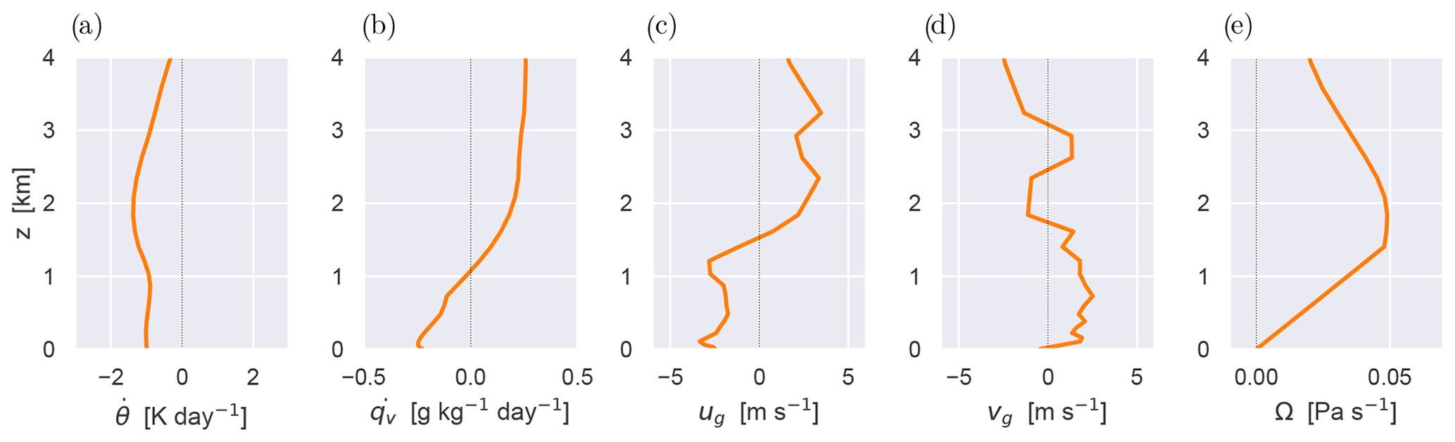
Table B1Overview of setting microphysical parameters for hydrometeors.
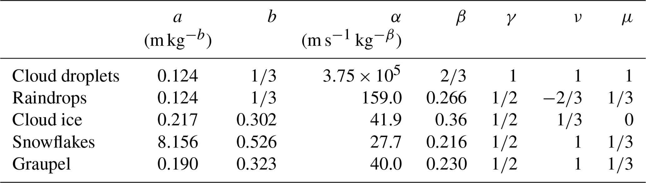
The overview covers the setting of microphysical parameters for the size and velocity of hydrometeors, as well as for particle mass distribution of hydrometeors under the assumption of a generalized gamma distribution.
B1 Nucleation of ice crystals
Ice nucleation in the bulk microphysics scheme of Seifert and Beheng (2006a) combines two previous approaches. Firstly, the number of activated ice nuclei is a function of supersaturation with respect to ice, as proposed by Meyers et al. (1992):
where T is the absolute temperature; Si is the supersaturation with respect to ice surface; the values of parameters follow number parameter NM=103 m−3, the intercept coefficient , the linear coefficient bM=12.96; and finally the threshold TM=268.15 K limits below which temperatures does the ice nucleation occur. Secondly, in order to avoid very low number concentrations, the nucleation is limited to be within 1 order of magnitude from the modified Fletcher's formula (Fletcher, 1962; Reisner et al., 1998):
where T0 is the freezing point of water and Tmin=246 K limits production at extremely low temperatures.
B2 Freezing of hydrometeors
The timescale in the heterogeneous freezing of supercooled cloud droplets is dependent on their size and temperature, following Pruppacher and Klett (1997) and Khain et al. (2000). The timescale in the homogeneous freezing of cloud droplets is then given by Cotton and Field (2002). The heterogeneous freezing of raindrops is analogous to the heterogeneous freezing of cloud droplets. The only difference lies in classifying the resulting particle as graupel.
B3 Secondary ice production
The secondary ice production includes ice multiplication by the Hallett–Mossop process, occurring during the riming of ice hydrometeors in the temperature ranges between 265 and 270 K (Hallett and Mossop, 1974; Griggs and Choularton, 1986). The number of ice splinters released during the process is dependent on the temperature and the riming rate, following the parameterization of Beheng (1982).
B4 Nucleation of cloud droplets
The nucleation of cloud droplets again follows Seifert and Beheng (2006a) as closely as possible. Firstly, the nucleation rate is calculated explicitly as
where Cccn and κ are CCN parameters, Sl is supersaturation with respect to liquid water surface (expressed in %), w is the vertical velocity of the air, and Smax is a threshold for saturation when all available CCN are activated. Secondly, the nucleation rate is limited so the number of droplets does not exceed Nccn, the current CCN number concentration. While RF20 reflects maritime conditions, the values of the κ parameter and the saturation threshold are set to constant values of κ=0.462 and Smax=1.1 % (Seifert and Beheng, 2006a). Unlike in the original description, the parameter is not the constant Cccn, but it is instead dependent on the aforementioned variable Nccn. The consistency with the power law relation for activation spectra is maintained by calculating this parameter as
The values of other important microphysical parameters are shown in Table B1.
The current version of DALES (https://doi.org/10.5281/zenodo.5642477; van Heerwaarden et al., 2021: DALES 4.3 with extension for an mixed-phase microphysics) is available on GitHub at https://github.com/jchylik/dales/releases/tag/dales4.3sb3cgn (Chylik, 2021). The aerosol dataset is available through the PANGAEA database at https://doi.org/10.1594/PANGAEA.900403 (Mertes et al., 2019). The files containing the ACLOUD RF20 case configuration, as well as the main model output, are available at https://doi.org/10.5281/zenodo.6565014 (Chylik et al., 2021).
SM provided the aerosols field measurements, as well as the guidelines on the treatment of aerosols. RN designed the model framework and strategy and prepared the model forcing files. JC developed the model extension for the interaction of aerosols and mixed-phase microphysics. MM operated the radar and lidar and performed measurements. BK provided the lidar data. MM and BK advised on the visualization and interpretation of remote sensing data. JC collected the ACLOUD observational datasets, performed the model simulations, and processed the output. RD provided guidelines on the treatment of in situ cloud measurements. CL and DC provided guidelines on the other airborne instruments, as well as the description of the field campaign. JC and RN worked together on analyzing the results and evaluating them against the measurements. JC prepared the manuscript, of which RN revised various intermediate versions.
The contact author has declared that none of the authors has any competing interests.
Publisher's note: Copernicus Publications remains neutral with regard to jurisdictional claims in published maps and institutional affiliations.
This article is part of the special issue “Arctic mixed-phase clouds as studied during the ACLOUD/PASCAL campaigns in the framework of (AC)3 (ACP/AMT/ESSD inter-journal SI)”. It is not associated with a conference.
We gratefully acknowledge the funding by the Deutsche Forschungsgemeinschaft (DFG, German Research Foundation) within the Transregional Collaborative Research Centre ArctiC Amplification: Climate Relevant Atmospheric and SurfaCe Processes and Feedback Mechanisms (AC)3 (grant no. 268020496, TRR 172). We thank ECMWF for providing access to the large-scale model analyses and forecasts fields used to drive the LES experiments. We gratefully acknowledge the Regional Computing Centre of the University of Cologne (RRZK) for granting us access to the CHEOPS cluster. The Gauss Centre for Supercomputing e.V. (https://www.gauss-centre.eu/, last access: 20 July 2022) is acknowledged for providing computing time on the Gauss Centre for Supercomputing (GCS) supercomputer JUWELS at the Jülich Supercomputing Centre (JSC) under projects CHKU28 and VIRTUALLAB. We further thank the Alfred Wegener Institute (AWI), the PS106/1 crew, and the ACLOUD science teams for making the field campaign happen and for post-processing the observational data.
This research has been supported by the Deutsche Forschungsgemeinschaft (grant no. 268020496, TRR 172).
This paper was edited by Radovan Krejci and reviewed by Ian Brooks and one anonymous referee.
Albrecht, B. A., Betts, A. K., Schubert, W. H., and Cox, S. K.: Model of the thermodynamic structure of the trade-wind boundary layer: Part I. Theoretical formulation and sensitivity tests, J. Atmos. Sci., 36, 73–89, 1979. a
Atkinson, B. W. and Wu Zhang, J.: Mesoscale shallow convection in the atmosphere, Rev. Geophys., 34, 403–431, https://doi.org/10.1029/96RG02623, 1996. a
Barnes, E. A. and Screen, J. A.: The impact of Arctic warming on the midlatitude jet-stream: Can it? Has it? Will it?, WIREs Clim. Change, 6, 277–286, https://doi.org/10.1002/wcc.337, 2015. a
Beheng, K. D.: A numerical study on the combined action of droplet coagulation, ice particle riming and the splintering process concerning maritime cumuli, Beit. Phys. Atmos., 55, 201–214, 1982. a, b
Bennartz, R., Shupe, M. D., Turner, D. D., Walden, V. P., Steffen, K., Cox, C. J., Kulie, M. S., Miller, N. B., and Pettersen, C.: July 2012 Greenland melt extent enhanced by low-level liquid clouds, Nature, 496, 83–86, https://doi.org/10.1038/nature12002, 2013. a
Bigg, E. K.: The formation of atmospheric ice crystals by the freezing of droplets, Q. J. Roy. Meteorol. Soc., 79, 510–519, https://doi.org/10.1002/qj.49707934207, 1953. a
Bigg, E. K. and Leck, C.: Cloud-active particles over the central Arctic Ocean, J. Geophys. Res.-Atmos., 106, 32155–32166, https://doi.org/10.1029/1999JD901152, 2001. a
Bigg, E. K., Leck, C., and Nilsson, E. D.: Sudden changes in arctic atmospheric aerosol concentrations during summer and autumn, Tellus B, 48, 254–271, https://doi.org/10.1034/j.1600-0889.1996.t01-1-00009.x, 1996. a, b
Brown, P. R. A. and Francis, P. N.: Improved Measurements of the Ice Water Content in Cirrus Using a Total-Water Probe, J. Atmos. Ocean. Tech., 12, 410–414, https://doi.org/10.1175/1520-0426(1995)012<0410:IMOTIW>2.0.CO;2, 1995. a
Browse, J., Carslaw, K. S., Mann, G. W., Birch, C. E., Arnold, S. R., and Leck, C.: The complex response of Arctic aerosol to sea-ice retreat, Atmos. Chem. Phys/, 14, 7543–7557, https://doi.org/10.5194/acp-14-7543-2014, 2014. a, b
Cai, Y., Montague, D. C., Mooiweer-Bryan, W., and Deshler, T.: Performance characteristics of the ultra high sensitivity aerosol spectrometer for particles between 55 and 800 nm: Laboratory and field studies, J. Aerosol Sci., 39, 759–769, https://doi.org/10.1016/j.jaerosci.2008.04.007, 2008. a
Chechin, D.: Liquid water content measured by the Nevzorov probe during the aircraft ACLOUD campaign in the Arctic, PANGAEA [data set], https://doi.org/10.1594/PANGAEA.906658, 2019. a
Chlond, A.: Three-dimensional simulation of cloud street development during a cold air outbreak, Bound.-Lay. Meteorol., 58, 161–200, https://doi.org/10.1007/BF00120757, 1992. a
Chylik, J.: Dales, Github [code], https://github.com/jchylik/dales/releases/tag/dales4.3sb3cgn, last access: 8 November 2021. a
Chylik, J., Chechin, D., Dupuy, R., Kulla, B. S., Lüpkes, C., Mertes, S., Mech, M., and Neggers, R. A. J.: Case simulation: LES RF20 composite case [Data set], Zenodo [data set], https://doi.org/10.5281/zenodo.6565014, 2021. a
Corbetta, G., Orlandi, E., Heus, T., Neggers, R., and Crewell, S.: Overlap statistics of shallow boundary layer clouds: Comparing ground-based observations with large-eddy simulations, Geophys. Res. Lett., 42, 8185–8191, https://doi.org/10.1002/2015GL065140, 2015. a
Cotton, R. J. and Field, P. R.: Ice nucleation characteristics of an isolated wave cloud, Q. J. Roy. Meteorol. Soc., 128, 2417–2437, https://doi.org/10.1256/qj.01.150, 2002. a
de Roode, S. R., Sandu, I., van der Dussen, J. J., Ackerman, A. S., Blossey, P., Jarecka, D., Lock, A., Siebesma, A. P., and Stevens, B.: Large-Eddy Simulations of EUCLIPSE-GASS Lagrangian Stratocumulus-to-Cumulus Transitions: Mean State, Turbulence, and Decoupling, J. Atmos. Res., 73, 2485–2508, https://doi.org/10.1175/JAS-D-15-0215.1, 2016. a
de Roode, S. R., Frederikse, T., Siebesma, A. P., Ackerman, A. S., Chylik, J., Field, P. R., Fricke, J., Gryschka, M., Hill, A., Honnert, R., Krueger, S. K., Lac, C., Lesage, A. T., and Tomassini, L.: Turbulent Transport in the Gray Zone: A Large Eddy Model Intercomparison Study of the CONSTRAIN Cold Air Outbreak Case, J. Adv. Model. Earth Syst., 11, 597–623, https://doi.org/10.1029/2018MS001443, 2019. a, b, c, d, e
Douglas, A. and L'Ecuyer, T.: Global evidence of aerosol-induced invigoration in marine cumulus clouds, Atmos. Chem. Phys., 21, 15103–15114, https://doi.org/10.5194/acp-21-15103-2021, 2021. a
Dupuy, R., Jourdan, O., Mioche, G., Gourbeyre, C., Leroy, D., and Schwarzenböck, A.: CDP, CIP and PIP In-situ arctic cloud microphysical properties observed during ACLOUD-AC3 campaign in June 2017, PANGAEA [data set], https://doi.org/10.1594/PANGAEA.899074, 2019. a
Duynkerke, P. G., de Roode, S. R., van Zanten, M. C., Calvo, J., Cuxart, J., Cheinet, S., Chlond, A., Grenier, H., Jonker, P. J., Köhler, M., Lenderink, G., Lewellen, D., Lappen, C.-L., Lock, A. P., Moeng, C.-H., Müller, F., Olmeda, D., Piriou, J.-M., Sánchez, E., and Sednev, I.: Observations and numerical simulations of the diurnal cycle of the EUROCS stratocumulus case, Q. J. Roy. Meteorol. Soc., 130, 3269–3296, https://doi.org/10.1256/qj.03.139, 2004. a
Egerer, U., Ehrlich, A., Gottschalk, M., Griesche, H., Neggers, R. A. J., Siebert, H., and Wendisch, M.: Case study of a humidity layer above Arctic stratocumulus and potential turbulent coupling with the cloud top, Atmos. Chem. Phys., 21, 6347–6364, https://doi.org/10.5194/acp-21-6347-2021, 2021. a
Ehrlich, A., Stapf, J., Lüpkes, C., Mech, M., Crewell, S., and Wendisch, M.: Meteorological measurements by dropsondes released from POLAR 5 during ACLOUD 2017, PANGAEA [data set], https://doi.org/10.1594/PANGAEA.900204, 2019a. a
Ehrlich, A., Wendisch, M., Lüpkes, C., Buschmann, M., Bozem, H., Chechin, D., Clemen, H.-C., Dupuy, R., Eppers, O., Hartmann, J., Herber, A., Jäkel, E., Järvinen, E., Jourdan, O., Kästner, U., Kliesch, L.-L., Köllner, F., Mech, M., Mertes, S., Neuber, R., Ruiz-Donoso, E., Schnaiter, M., Schneider, J., Stapf, J., and Zanatta, M.: Collection of data sources for the Arctic CLoud Observations Using airborne measurements during polar Day (ACLOUD) campaign, North-West of Svalbard between 23 May–26 June 2017, PANGAEA [data set], https://doi.org/10.1594/PANGAEA.902603, 2019b. a
Fletcher, J. K., Mason, S., and Jakob, C.: A Climatology of Clouds in Marine Cold Air Outbreaks in Both Hemispheres, J. Climate, 29, 6677–6692, https://doi.org/10.1175/JCLI-D-15-0783.1, 2016. a
Fletcher, N. H.: The physics of rainclouds, Cambridge University Press, https://doi.org/10.1002/qj.49708837821, 1962. a
Garrett, T., Zhao, C., and Novelli, P.: Assessing the relative contributions of transport efficiency and scavenging to seasonal variability in Arctic aerosol, Tellus B, 62, 190–196, https://doi.org/10.1111/j.1600-0889.2010.00453.x, 2010. a
Garrett, T. J., Radke, L. F., and Hobbs, P. V.: Aerosol Effects on Cloud Emissivity and Surface Longwave Heating in the Arctic, J. Atmos. Sci., 59, 769–778, https://doi.org/10.1175/1520-0469(2002)059<0769:AEOCEA>2.0.CO;2, 2002. a
Georgakaki, P., Sotiropoulou, G., Vignon, E., Billault-Roux, A.-C., Berne, A., and Nenes, A.: Secondary ice production processes in wintertime alpine mixed-phase clouds, Atmos. Chem. Phys., 22, 1965–1988, https://doi.org/10.5194/acp-22-1965-2022, 2022. a
Griggs, D. J. and Choularton, T. W.: The effect of rimer surface temperature on ice splinter production by the Hallett-Mossop process, Q. J. Roy. Meteorol. Soc., 112, 1254–1256, https://doi.org/10.1002/qj.49711247419, 1986. a, b
Gryschka, M. and Raasch, S.: Roll convection during a cold air outbreak: A large eddy simulation with stationary model domain, Geophys. Res. Lett., 32, L14805, https://doi.org/10.1029/2005GL022872, 2005. a
Hallett, J. and Mossop, S.: Production of secondary ice particles during the riming process, Nature, 249, 26–28, https://doi.org/10.1038/249026a0, 1974. a, b, c
Hartmann, J., Gehrmann, M., Kohnert, K., Metzger, S., and Sachs, T.: New calibration procedures for airborne turbulence measurements and accuracy of the methane fluxes during the AirMeth campaigns, Atmos. Meas. Tech., 11, 4567–4581, https://doi.org/10.5194/amt-11-4567-2018, 2018. a
Hartmann, J., Lüpkes, C., and Chechin, D.: High resolution aircraft measurements of wind and temperature during the ACLOUD campaign in 2017, PANGAEA [data set], https://doi.org/10.1594/PANGAEA.900880, 2019. a
Hartmann, M., Blunier, T., Brügger, S., Schmale, J., Schwikowski, M., Vogel, A., Wex, H., and Stratmann, F.: Variation of Ice Nucleating Particles in the European Arctic Over the Last Centuries, Geophys. Res. Lett., 46, 4007–4016, https://doi.org/10.1029/2019GL082311, 2019. a, b
Heus, T., van Heerwaarden, C. C., Jonker, H. J. J., Siebesma, A. P., Axelsen, S., van den Dries, K., Geoffroy, O., Moene, A. F., Pino, D., de Roode, S. R., and de Arellano, J. V.-G.: Formulation of the Dutch Atmospheric Large-Eddy Simulation (DALES) and overview of its applications, Geosci. Model Dev., 3, 415–444, https://doi.org/10.5194/gmd-3-415-2010, 2010. a, b, c, d, e
Im, U., Tsigaridis, K., Faluvegi, G., Langen, P. L., French, J. P., Mahmood, R., Thomas, M. A., von Salzen, K., Thomas, D. C., Whaley, C. H., Klimont, Z., Skov, H., and Brandt, J.: Present and future aerosol impacts on Arctic climate change in the GISS-E2.1 Earth system model, Atmos. Chem. Phys., 21, 10413–10438, https://doi.org/10.5194/acp-21-10413-2021, 2021. a
Ito, A. and Kawamiya, M.: Potential impact of ocean ecosystem changes due to global warming on marine organic carbon aerosols, Global Biogeochem. Cy., 24, GB1012, https://doi.org/10.1029/2009GB003559, 2010. a
Jenkins, M. and Dai, A.: The Impact of Sea-Ice Loss on Arctic Climate Feedbacks and Their Role for Arctic Amplification, Geophys. Res. Lett., 48, e2021GL094599, https://doi.org/10.1029/2021GL094599, 2021. a
Khain, A., Ovtchinnikov, M., Pinsky, M., Pokrovsky, A., and Krugliak, H.: Notes on the state-of-the-art numerical modeling of cloud microphysics, Atmos. Res., 55, 159–224, https://doi.org/10.1016/S0169-8095(00)00064-8, 2000. a
Klein, S. A., McCoy, R. B., Morrison, H., Ackerman, A. S., Avramov, A., de Boer, G., Chen, M., Cole, J. N. S., Del Genio, A. D., Falk, M., Foster, M. J., Fridlind, A., Golaz, J.-C., Hashino, T., Harrington, J. Y., Hoose, C., Khairoutdinov, M. F., Larson, V. E., Liu, X., Luo, Y., McFarquhar, G. M., Menon, S., Neggers, R. A. J., Park, S., Poellot, M. R., Schmidt, J. M., Sednev, I., Shipway, B. J., Shupe, M. D., Spangenberg, D. A., Sud, Y. C., Turner, D. D., Veron, D. E., von Salzen, K., Walker, G. K., Wang, Z., Wolf, A. B., Xie, S., Xu, K.-M., Yang, F., and Zhang, G.: Intercomparison of model simulations of mixed-phase clouds observed during the ARM Mixed-Phase Arctic Cloud Experiment. I: single-layer cloud, Q. J. Roy. Meteorol. Soc., 135, 979–1002, https://doi.org/10.1002/qj.416, 2009. a
Kliesch, L.-L. and Mech, M.: Airborne radar reflectivity and brightness temperature measurements with POLAR 5 during ACLOUD in May and June 2017, https://doi.org/10.1594/PANGAEA.899565, supplement to: Mech, Mario; Kliesch, Leif-Leonard; Anhäuser, Andreas; Rose, Thomas; Kollias, Pavlos; Crewell, Susanne (2019): Microwave Radar/radiometer for Arctic Clouds (MiRAC): first insights from the ACLOUD campaign, Atmos. Meas. Tech., 12, 5019–5037, https://doi.org/10.5194/amt-12-5019-2019, 2019. a
Knudsen, E. M., Heinold, B., Dahlke, S., Bozem, H., Crewell, S., Gorodetskaya, I. V., Heygster, G., Kunkel, D., Maturilli, M., Mech, M., Viceto, C., Rinke, A., Schmithüsen, H., Ehrlich, A., Macke, A., Lüpkes, C., and Wendisch, M.: Meteorological conditions during the ACLOUD/PASCAL field campaign near Svalbard in early summer 2017, Atmos. Chem. Phys., 18, 17995–18022, https://doi.org/10.5194/acp-18-17995-2018, 2018. a, b, c
Kretzschmar, J., Stapf, J., Klocke, D., Wendisch, M., and Quaas, J.: Employing airborne radiation and cloud microphysics observations to improve cloud representation in ICON at kilometer-scale resolution in the Arctic, Atmos. Chem. Phys., 20, 13145–13165, https://doi.org/10.5194/acp-20-13145-2020, 2020. a
Lauer, M., Block, K., Salzmann, M., and Quaas, J.: CO2-forced changes of Arctic temperature lapse rates in CMIP5 models, Meteorol. Z., 29, 79–93, https://doi.org/10.1127/metz/2020/0975, 2020. a
Liu, Y., Key, J. R., Liu, Z., Wang, X., and Vavrus, S. J.: A cloudier Arctic expected with diminishing sea ice, Geophys. Res. Lett., 39, L05705, https://doi.org/10.1029/2012GL051251, 2012. a
Liu, Y., Key, J. R., Vavrus, S., and Woods, C.: Time Evolution of the Cloud Response to Moisture Intrusions into the Arctic during Winter, J. Climate, 31, 9389–9405, https://doi.org/10.1175/JCLI-D-17-0896.1, 2018. a
Macke, A. and Flores, H.: The Expeditions PS106/1 and 2 of the Research Vessel POLARSTERN to the Arctic Ocean in 2017, Reports on Polar and Marine Research, AWI – Alfred Wegener Institute, Bremerhaven, Germany, 719, 171, https://doi.org/10.2312/BzPM_0719_2018, 2018. a
Markowicz, K., Lisok, J., and Xian, P.: Simulation of long-term direct aerosol radiative forcing over the arctic within the framework of the iAREA project, Atmos. Environ., 244, 117882, https://doi.org/10.1016/j.atmosenv.2020.117882, 2021. a
Mauritsen, T., Sedlar, J., Tjernström, M., Leck, C., Martin, M., Shupe, M., Sjogren, S., Sierau, B., Persson, P. O. G., Brooks, I. M., and Swietlicki, E.: An Arctic CCN-limited cloud-aerosol regime, Atmos. Chem. Phys., 11, 165–173, https://doi.org/10.5194/acp-11-165-2011, 2011. a
Mech, M., Kliesch, L.-L., Anhäuser, A., Rose, T., Kollias, P., and Crewell, S.: Microwave Radar/Radiometer for Arctic Clouds (MiRAC): First Insights from the ACLOUD Campaign, Atmos. Meas. Tech., 12, 5019–5037, https://doi.org/10.5194/amt-12-5019-2019, 2019. a
Mertes, S., Kästner, U., and Macke, A.: Airborne in-situ measurements of the aerosol absorption coefficient, aerosol particle number concentration and size distribution of cloud particle residuals and ambient aerosol particles during flight P6_206_ACLOUD_2017_1706181901, PANGAEA, https://doi.org/10.1594/PANGAEA.900394, in: Mertes, S., et al. (2019): Airborne in-situ measurements of the aerosol absorption coefficient, aerosol particle number concentration and size distribution of cloud particle residuals and ambient aerosol particles during the ACLOUD campaign in May and June 2017, Leibniz-Institut für Troposphärenforschung e.V., Leipzig, PANGAEA [data set], https://doi.org/10.1594/PANGAEA.900403 2019. a, b, c, d
Meyers, M. P., DeMott, P. J., and Cotton, W. R.: New Primary Ice-Nucleation Parameterizations in an Explicit Cloud Model, J. Appl. Meteorol., 31, 708–721, https://doi.org/10.1175/1520-0450(1992)031<0708:NPINPI>2.0.CO;2, 1992. a
Morrison, H., McCoy, R. B., Klein, S. A., Xie, S., Luo, Y., Avramov, A., Chen, M., Cole, J. N. S., Falk, M., Foster, M. J., Del Genio, A. D., Harrington, J. Y., Hoose, C., Khairoutdinov, M. F., Larson, V. E., Liu, X., McFarquhar, G. M., Poellot, M. R., von Salzen, K., Shipway, B. J., Shupe, M. D., Sud, Y. C., Turner, D. D., Veron, D. E., Walker, G. K., Wang, Z., Wolf, A. B., Xu, K.-M., Yang, F., and Zhang, G.: Intercomparison of model simulations of mixed-phase clouds observed during the ARM Mixed-Phase Arctic Cloud Experiment. II: Multilayer cloud, Q. J. Roy. Meteorol. Soc., 135, 1003–1019, https://doi.org/10.1002/qj.415, 2009. a
Morrison, H., de Boer, G., Feingold, G., Harrington, J., Shupe, M. D., and Sulia, K.: Resilience of persistent Arctic mixed-phase clouds, Nat. Geosci., 5, 11–17, https://doi.org/10.1038/NGEO1332, 2012. a
Müller, G., Brümmer, B., and Alpers, W.: Roll Convection within an Arctic Cold-Air Outbreak: Interpretation of In Situ Aircraft Measurements and Spaceborne SAR Imagery by a Three-Dimensional Atmospheric Model, Mon. Weather Rev., 127, 363–380, https://doi.org/10.1175/1520-0493(1999)127<0363:RCWAAC>2.0.CO;2, 1999. a, b
Neggers, R. A. J.: LES results to accompany measurements at the POLARSTERN Research Vessel during the PASCAL field campaign on 6 June 2017, PANGAEA [data set], https://doi.pangaea.de/10.1594/PANGAEA.919945, 2020a. a
Neggers, R. A. J.: LES results to accompany measurements at the POLARSTERN Research Vessel during the PASCAL field campaign on 7 June 2017, PANGAEA [data set], https://doi.pangaea.de/10.1594/PANGAEA.919946, 2020b. a
Neggers, R. A. J., Siebesma, A. P., and Heus, T.: Continuous Single-Column Model Evaluation at a Permanent Meteorological Supersite, B. Am. Meteorol. Soc., 93, 1389–1400, https://doi.org/10.1175/BAMS-D-11-00162.1, 2012. a, b
Neggers, R. A. J., Chylik, J., Egerer, U., Griesche, H., Schemann, V., Seifert, P., Siebert, H., and Macke, A.: Local and Remote Controls on Arctic Mixed-Layer Evolution, J. Adv. Model. Earth Syst., 11, 2214–2237, https://doi.org/10.1029/2019MS001671, 2019. a, b, c, d, e, f
Neuber, R., Schmidt, L. V., Ritter, C., and Mech, M.: Cloud top altitudes observed with airborne lidar during flight P5_206_ACLOUD_2017_1706182001, PANGAEA, https://doi.org/10.1594/PANGAEA.899952, in: Neuber, R., et al. (2019): Cloud top altitudes observed with airborne lidar during the ACLOUD campaign, Alfred Wegener Institute – Research Unit Potsdam, PANGAEA [data set], https://doi.org/10.1594/PANGAEA.899962, 2019. a
Nicholls, S.: The dynamics of stratocumulus: Aircraft observations and comparisons with a mixed layer model, Q. J. Roy. Meteorol. Soc., 110, 783–820, https://doi.org/10.1002/qj.49711046603, 1984. a
Nicholls, S. and Lemone, M. A.: The Fair Weather Boundary Layer in GATE: The Relationship of Subcloud Fluxes and Structure to the Distribution and Enhancement of Cumulus Clouds, J. Atmos. Sci. 37, 2051–2067, https://doi.org/10.1175/1520-0469(1980)037<2051:TFWBLI>2.0.CO;2, 1980. a
Ovchinnikov, M., Ackerman, A. S., Avramov, A., Cheng, A., Fan, J., Fridlind, A. M., Ghan, S., Harrington, J., Hoose, C., Korolev, A., McFarquhar, G. M., Morrison, H., Paukert, M., Savre, J., Shipway, B. J., Shupe, M. D., Solomon, A., and Sulia, K.: Intercomparison of large-eddy simulations of Arctic mixed-phase clouds: Importance of ice size distribution assumptions, J. Adv. Model. Earth Syst., 6, 223–248, https://doi.org/10.1002/2013MS000282, 2014. a, b
Overland, J. E., Wang, M., Walsh, J. E., and Stroeve, J. C.: Future Arctic climate changes: Adaptation and mitigation time scales, Earth's Future, 2, 68–74, https://doi.org/10.1002/2013EF000162, 2014. a
Perovich, D. K., Andreas, E. L., Curry, J. A., Eiken, H., Fairall, C. W., Grenfell, T. C., Guest, P., Intrieri, J., Kadko, D., Lindsay, R. W., McPhee, M. G., Morison, J., Moritz, R. E., Paulson, C. A., Pegau, W. S., Persson, P., Pinkel, R., Richter-Menge, J. A., Stanton, T., Stern, H., Sturm, M., Tucker III, W., and Uttal, T.: Year on ice gives climate insights, Eos Trans. Am. Geophys. Union, 80, 481–486, https://doi.org/10.1029/EO080i041p00481-01, 1999. a
Pincus, R. and Stevens, B.: Monte Carlo Spectral Integration: a Consistent Approximation for Radiative Transfer in Large Eddy Simulations, J. Adv. Model. Earth Syst., 1, https://doi.org/10.3894/JAMES.2009.1.1, 2009. a
Pithan, F. and Mauritsen, T.: Arctic amplification dominated by temperature feedbacks in contemporary climate models, Nat. Geosci., 7, 181–184, https://doi.org/10.1038/ngeo2071, 2014. a
Pithan, F., Svensson, G., Caballero, R., Chechin, D., Cronin, T. W., Ekman, A. M. L., Neggers, R., Shupe, M. D., Solomon, A., Tjernström, M., and Wendisch, M.: Role of air-mass transformations in exchange between the Arctic and mid-latitudes, Nat. Geosci., 11, 805–812, https://doi.org/10.1038/s41561-018-0234-1, 2018. a, b, c
Pruppacher, H. R. and Klett, J. D.: Microphysics of clouds and precipitation, Kluwer Academic Publishers, Dordrecht, https://doi.org/10.1080/02786829808965531, 1997. a
Reilly, S., Gesso, S. D., and Neggers, R.: Configuring LES Based on Dropsonde Data in Sparsely Sampled Areas in the Subtropical Atlantic, J. Appl. Meteorol. Clim., 59, 297–315, https://doi.org/10.1175/JAMC-D-19-0013.1, 2020. a
Reisner, J., Rasmussen, R. M., and Bruintjes, R. T.: Explicit forecasting of supercooled liquid water in winter storms using the MM5 mesoscale model, Q. J. Roy. Meteorol. Soc., 124, 1071–1107, https://doi.org/10.1002/qj.49712454804, 1998. a, b, c
Rinke, A., Maturilli, M., Graham, R. M., Matthes, H., Handorf, D., Cohen, L., Hudson, S. R., and Moore, J. C.: Extreme cyclone events in the Arctic: Wintertime variability and trends, Environ. Res. Lett., 12, 094006, https://doi.org/10.1088/1748-9326/aa7def, 2017. a
Rozendaal, M. A., Leovy, C. B., and Klein, S. A.: An Observational Study of Diurnal Variations of Marine Stratiform Cloud, J. Climate, 8, 1795–1809, https://doi.org/10.1175/1520-0442(1995)008<1795:AOSODV>2.0.CO;2, 1995. a
Ruiz-Donoso, E., Ehrlich, A., Schäfer, M., Jäkel, E., Schemann, V., Crewell, S., Mech, M., Kulla, B. S., Kliesch, L.-L., Neuber, R., and Wendisch, M.: Small-scale structure of thermodynamic phase in Arctic mixed-phase clouds observed by airborne remote sensing during a cold air outbreak and a warm air advection event, Atmos. Chem. Phys., 20, 5487–5511, https://doi.org/10.5194/acp-20-5487-2020, 2020. a
Sandu, I., Brenguier, J.-L., Thouron, O., and Stevens, B.: How important is the vertical structure for the representation of aerosol impacts on the diurnal cycle of marine stratocumulus?, Atmos. Chem. Phys., 9, 4039–4052, https://doi.org/10.5194/acp-9-4039-2009, 2009. a
Savtchenko, A., Ouzounov, D., Ahmad, S., Acker, J., Leptoukh, G., Koziana, J., and Nickless, D.: Terra and Aqua MODIS products available from NASA GES DAAC, Adv. Space Res., 34, 710–714, https://doi.org/10.1016/j.asr.2004.03.012, 2004. a
Schwarzenböck, A., Mertes, S., Heintzenberg, J., Wobrock, W., and Laj, P.: Impact of the Bergeron–Findeisen process on the release of aerosol particles during the evolution of cloud ice, Atmos. Res., 58, 295–313, https://doi.org/10.1016/S0169-8095(01)00096-5, 2001. a
Screen, J. A., Simmonds, I., Deser, C., and Tomas, R.: The Atmospheric Response to Three Decades of Observed Arctic Sea Ice Loss, J. Climate, 26, 1230–1248, https://doi.org/10.1175/JCLI-D-12-00063.1, 2013. a
Seifert, A. and Beheng, K. D.: A double-moment parameterization for simulating autoconversion, accretion and selfcollection, Atmos. Res., 59–60, 265–281, https://doi.org/10.1016/S0169-8095(01)00126-0, 2001. a
Seifert, A. and Beheng, K. D.: A two-moment cloud microphysics parameterization for mixed-phase clouds. Part 1: Model description, Meteorol. Atmos. Phys., 92, 45–66, https://doi.org/10.1007/s00703-005-0112-4, 2006a. a, b, c, d, e
Seifert, A. and Beheng, K. D.: A two-moment cloud microphysics parameterization for mixed-phase clouds. Part 2: Maritime vs. continental deep convective storms, Meteorol. Atmos. Phys., 92, 67–82, https://doi.org/10.1007/s00703-005-0113-3, 2006b. a
Shepherd, T. G., Semeniuk, K., and Koshyk, J. N.: Sponge layer feedbacks in middle-atmosphere models, J. Geophys. Res.-Atmos., 101, 23447–23464, https://doi.org/10.1029/96JD01994, 1996. a
Shupe, M. D., Rex, M., Dethloff, K., Damm, E., Fong, A. A., Gradinger, R., Heuze, C., Loose, B., Makarov, A., Maslowski, W., Nicolaus, M., Perovich, D., Rabe, B., Rinke, A., Sokolov, V., and Sommerfeld, A.: The MOSAiC Expedition: A Year Drifting with the Arctic Sea Ice, Arctic report card, NOAA, https://doi.org/10.25923/9g3v-xh92, 2021. a
Solomon, A., Shupe, M. D., Persson, O., Morrison, H., Yamaguchi, T., Caldwell, P. M., and de Boer, G.: The Sensitivity of Springtime Arctic Mixed-Phase Stratocumulus Clouds to Surface-Layer and Cloud-Top Inversion-Layer Moisture Sources, J. Atmos. Res., 71, 574–595, https://doi.org/10.1175/JAS-D-13-0179.1, 2014. a
Stachlewska, I. S., Neuber, R., Lampert, A., Ritter, C., and Wehrle, G.: AMALi – the Airborne Mobile Aerosol Lidar for Arctic research, Atmos. Chem. Phys., 10, 2947–2963, https://doi.org/10.5194/acp-10-2947-2010, 2010. a
Stevens, B., Moeng, C.-H., Ackerman, A. S., Bretherton, C. S., Chlond, A., de Roode, S., Edwards, J., Golaz, J.-C., Jiang, H., Khairoutdinov, M., Kirkpatrick, M. P., Lewellen, D. C., Lock, A., Müller, F., Stevens, D. E., Whelan, E., and Zhu, P.: Evaluation of Large-Eddy Simulations via Observations of Nocturnal Marine Stratocumulus, Mon. Weather Re., 133, 1443–1462, https://doi.org/10.1175/MWR2930.1, 2005. a, b, c
Stevens, R. G., Loewe, K., Dearden, C., Dimitrelos, A., Possner, A., Eirund, G. K., Raatikainen, T., Hill, A. A., Shipway, B. J., Wilkinson, J., Romakkaniemi, S., Tonttila, J., Laaksonen, A., Korhonen, H., Connolly, P., Lohmann, U., Hoose, C., Ekman, A. M. L., Carslaw, K. S., and Field, P. R.: A model intercomparison of CCN-limited tenuous clouds in the high Arctic, Atmos. Chem. Phys., 18, 11041–11071, https://doi.org/10.5194/acp-18-11041-2018, 2018. a, b, c
Stohl, A., Andrews, E., Burkhart, J. F., Forster, C., Herber, A., Hoch, S. W., Kowal, D., Lunder, C., Mefford, T., Ogren, J. A., Sharma, S., Spichtinger, N., Stebel, K., Stone, R., Ström, J., Tørseth, K., Wehrli, C., and Yttri, K. E.: Pan-Arctic enhancements of light absorbing aerosol concentrations due to North American boreal forest fires during summer 2004, J. Geophys. Res.-Atmos., 111, D22214, https://doi.org/10.1029/2006JD007216, 2006. a
Stull, R. B.: An introduction to boundary layer meteorology, in: vol. 13, Springer Science & Business Media, https://doi.org/10.1007/978-94-009-3027-8, 1988. a
Sullivan, S. C., Hoose, C., and Nenes, A.: Investigating the contribution of secondary ice production to in-cloud ice crystal numbers, J. Geophys. Res.-Atmos., 122, 9391–9412, https://doi.org/10.1002/2017JD026546, 2017. a
Tjernström, M., Birch, C. E., Brooks, I. M., Shupe, M. D., Persson, P. O. G., Sedlar, J., Mauritsen, T., Leck, C., Paatero, J., Szczodrak, M., and Wheeler, C. R.: Meteorological conditions in the central Arctic summer during the Arctic Summer Cloud Ocean Study (ASCOS), Atmos. Chem. Phys., 12, 6863–6889, https://doi.org/10.5194/acp-12-6863-2012, 2012. a
Twomey, S.: The Influence of Pollution on the Shortwave Albedo of Clouds, J. Atmos. Sci., 34, 1149–1152, https://doi.org/10.1175/1520-0469(1977)034<1149:TIOPOT>2.0.CO;2, 1977. a
Van der Dussen, J. J., de Roode, S. R., Ackerman, A. S., Blossey, P. N., Bretherton, C. S., Kurowski, M. J., Lock, A. P., Neggers, R. A. J., Sandu, I., and Siebesma, A. P.: The GASS/EUCLIPSE model intercomparison of the stratocumulus transition as observed during ASTEX: LES results, J. Adv. Model. Earth Syst., 5, 483–499, https://doi.org/10.1002/jame.20033, 2013. a
van Heerwaarden, C., sjboeing, Ouwersloot, H., thijsheus, Attema, J., Jansson, F., Arabas, S., Vila, J., sderoode, afmoene, and van Stratum, B.: jchylik/dales: Dales4.3_sb3 (dales4.3sb3cgn), Zenodo [code], https://doi.org/10.5281/zenodo.5642477, 2021. a
Van Laar, T. W., Schemann, V., and Neggers, R. A. J.: Investigating the diurnal evolution of the cloud size distribution of continental cumulus convection using multi-day LES, J. Atmos. Sci., 76, 729–747, https://doi.org/10.1175/JAS-D-18-0084.1, 2019. a, b, c
Vázquez, M., Nieto, R., Drumond, A., and Gimeno, L.: Moisture transport into the Arctic: Source-receptor relationships and the roles of atmospheric circulation and evaporation, J. Geophys. Res.-Atmos., 121, 13,493–13,509, https://doi.org/10.1002/2016JD025400, 2016. a
Vilà-Guerau de Arellano, J., Wang, X., Pedruzo-Bagazgoitia, X., Sikma, M., Agustí-Panareda, A., Boussetta, S., Balsamo, G., Machado, L. A. T., Biscaro, T., Gentine, P., Martin, S. T., Fuentes, J. D., and Gerken, T.: Interactions Between the Amazonian Rainforest and Cumuli Clouds: A Large-Eddy Simulation, High-Resolution ECMWF, and Observational Intercomparison Study, J. Adv. Model. Earth Syst., 12, e2019MS001828, https://doi.org/10.1029/2019MS001828, 2020. a
Wendisch, M., Macke, A., Ehrlich, A., Lüpkes, C., Mech, M., Chechin, D., Dethloff, K., Velasco, C. B., Bozem, H., Brückner, M., Clemen, H.-C., Crewell, S., Donth, T., Dupuy, R., Ebell, K., Egerer, U., Engelmann, R., Engler, C., Eppers, O., Gehrmann, M., Gong, X., Gottschalk, M., Gourbeyre, C., Griesche, H., Hartmann, J., Hartmann, M., Heinold, B., Herber, A., Herrmann, H., Heygster, G., Hoor, P., Jafariserajehlou, S., Jäkel, E., Järvinen, E., Jourdan, O., Kästner, U., Kecorius, S., Knudsen, E. M., Köllner, F., Kretzschmar, J., Lelli, L., Leroy, D., Maturilli, M., Mei, L., Mertes, S., Mioche, G., Neuber, R., Nicolaus, M., Nomokonova, T., Notholt, J., Palm, M., van Pinxteren, M., Quaas, J., Richter, P., Ruiz-Donoso, E., Schäfer, M., Schmieder, K., Schnaiter, M., Schneider, J., Schwarzenböck, A., Seifert, P., Shupe, M. D., Siebert, H., Spreen, G., Stapf, J., Stratmann, F., Vogl, T., Welti, A., Wex, H., Wiedensohler, A., Zanatta, M., and Zeppenfeld, S.: The Arctic Cloud Puzzle: Using ACLOUD/PASCAL Multiplatform Observations to Unravel the Role of Clouds and Aerosol Particles in Arctic Amplification, B. Am. Meteorol. Soc., 100, 841–871, https://doi.org/10.1175/BAMS-D-18-0072.1, 2019. a, b, c
Wendisch, M. E. A.: Understanding causes and effects of rapid warming in the Arctic, Eos Trans. Am. Geophys. Union, 98, 22–26, https://doi.org/10.1029/2017EO064803, 2017. a
Wesche, C., Steinhage, D., and Nixdorf, U.: Polar aircraft Polar5 and Polar6 operated by the Alfred Wegener Institute, J. Large-scale Res. Facil., 2, 1–7, https://doi.org/10.17815/jlsrf-2-153, 2016. a
Wood, R., Bretherton, C. S., and Hartmann, D. L.: Diurnal cycle of liquid water path over the subtropical and tropical oceans, Geophys. Res. Lett., 29, 7-1–7-4, https://doi.org/10.1029/2002GL015371, 2002. a
Yang, Y. and Liu, R.: Anthropogenic Aerosols Effects on Ice Clouds: A Review, Atmosphere, 13, 910, https://doi.org/10.3390/atmos13060910, 2022. a
Zanatta, M. and Herber, A.: Aircraft measurements of aerosol size distribution in the Arctic during flight P6_206_ACLOUD_2017_1706181901 of the ACLOUD campaign 2017, PANGAEA, https://doi.org/10.1594/PANGAEA.900335, in: Zanatta, M. and Herber, A. (2019): Aircraft measurements of aerosol size distribution in the Arctic during the ACLOUD campaign 2017, Alfred Wegener Institute, Helmholtz Centre for Polar and Marine Research, Bremerhaven, PANGAEA, PANGAEA [data set], https://doi.org/10.1594/PANGAEA.900341, 2019. a, b, c
- Abstract
- Introduction
- Observations
- Model configuration
- Results I: evaluation
- Results II: aerosol impacts
- Discussion
- Conclusions and outlook
- Appendix A: Composite forcings
- Appendix B: Microphysics scheme
- Code and data availability
- Author contributions
- Competing interests
- Disclaimer
- Special issue statement
- Acknowledgements
- Financial support
- Review statement
- References