Ice-nucleating particles in northern Greenland: annual cycles, biological contribution and parameterizations

Ice-nucleating particles (INPs) can initiate ice formation in clouds at temperatures above −38 ^∘C through heterogeneous ice nucleation. As a result, INPs affect cloud microphysical and radiative properties, cloud lifetime, and precipitation behavior and thereby ultimately the Earth's climate. Yet, little is known regarding the sources, abundance and properties of INPs, especially in remote regions such as the Arctic. In this study, 2-year-long INP measurements (from July 2018 to September 2020) at Villum Research Station in northern Greenland are presented. A low-volume filter sampler was deployed to collect filter samples for offline INP analysis. An annual cycle of INP concentration (N_INP) was observed, and the fraction of heat-labile INPs was found to be higher in months with low to no snow cover and lower in months when the surface was well covered in snow (> 0.8 m). Samples were categorized into three different types based only on the slope of their INP spectra, namely into summer, winter and mix type. For each of the types a temperature-dependent INP parameterization was derived, clearly different depending on the time of the year. Winter and summer types occurred only during their respective seasons and were seen 60 % of the time. The mixed type occurred in the remaining 40 % of the time throughout the year. April, May and November were found to be transition months. A case study comparing April 2019 and April 2020 was performed. The month of April was selected because a significant difference in N_INP was observed during these two periods, with clearly higher N_INP in April 2020. In parallel to the observed differences in N_INP, also a higher cloud-ice fraction was observed in satellite data for April 2020, compared to April 2019. N_INP in the case study period revealed no clear dependency on either meteorological parameters or different surface types which were passed by the collected air masses. Overall, the results suggest that the coastal regions of Greenland were the main sources of INPs in April 2019 and 2020, most likely including both local terrestrial and marine sources.

1 Introduction

The Arctic is known to be one of the most sensitive regions on Earth, where climate change takes place at an unexpectedly intense pace (Cohen et al., 2014; Serreze and Barry, 2011; Morrison et al., 2012). In the last 2 decades, the Arctic near-surface air temperature has increased almost 4 times as fast as that of the rest of the globe (Rantanen et al., 2022). This phenomenon is usually referred to as Arctic amplification (AA) (Wendisch et al., 2017; Cohen et al., 2014). Different effects and feedbacks such as surface albedo effect, water vapor, lapse rate and cloud feedback have been studied and identified as potential contributors to AA (Wendisch et al., 2017). However, the combined effects and their relative importance to the Arctic region, as well as their influence on the midlatitude weather, are still unclear (Pithan and Mauritsen, 2014; Cohen et al., 2020).

Aerosol particles are an important component in the climate system. They can directly scatter and/or absorb radiation (Myhre et al., 2013; Boucher et al., 2013) as well as affect the energy budget of the Arctic boundary layer by altering the microphysical properties of clouds (Morrison et al., 2012; Pruppacher and Klett, 2010). Arctic clouds are often low-level, persistent and form stratiform layers (Shupe et al., 2006). They tend to cause a net warming effect for the underlying surface in comparison to clear sky condition, due to the upward longwave radiation reflected downward by the cloud (Intrieri et al., 2002; Shupe and Intrieri, 2004). This can increase the sea-ice melt (Vavrus et al., 2011) and facilitate biological activities in the ocean, which then can contribute to and change the Arctic aerosol population (Creamean et al., 2019; McCluskey et al., 2017). Analogous to the marine environment, it is expected that the terrestrial ecosystem will respond to longer snow-free periods with enhanced biological activity (Cooper, 2014). This may lead to more primary biological aerosol particles directly emitted from plants, such as pollen and spores. Also, exposure of non-snow-covered surfaces to the atmosphere will likely enhance emission of soil dust, and therewith could largely contribute to ice-nucleating particles (INPs) (Šantl Temkiv et al., 2019; Sanchez-Marroquin et al., 2020; Tobo et al., 2019). As the Arctic is warming, the permafrost is also expected to thaw, promoting microbial metabolic activity in the soil (Wild et al., 2019; Schuur et al., 2015), which could then be mobilized in the atmosphere as well (Creamean et al., 2020).

Clouds in the Arctic are usually mixed-phase (Shupe et al., 2006), i.e., contain both supercooled liquid droplets and ice crystals. Primary ice formation in the atmosphere can happen via homogeneous nucleation at −38 ^∘C or below or via heterogeneous nucleation where aerosol particles, the already mentioned INPs, act as catalysts at any temperature below 0 ^∘C (Vali et al., 2015). Immersion freezing is arguably the most relevant freezing mechanism in the Arctic mixed-phase clouds (MPCs) regime, which requires INPs immersed into cloud droplets (Boer et al., 2011; Hande and Hoose, 2017). By inducing the ice formation in MPCs, the presence of INPs can alter the number and size of liquid droplets and ice crystals in a cloud through, e.g., the Wegener–Bergeron–Findeisen process. Connected to this, for Arctic MPCs at temperatures above −10 ^∘C, it was recently observed that they contain heterogeneously formed ice 2 to 6 times more often when they were coupled to the surface, compared to decoupled clouds (Griesche et al., 2021). Ultimately, INPs affect the radiative properties, life time and precipitation formation in the clouds (Kanji et al., 2017; Hoose and Möhler, 2012; Murray et al., 2012).

The ability of aerosol particles acting as INPs largely depends on their size, morphology, composition and source (Hoose and Möhler, 2012). However, correlating INP concentration with physical properties of the bulk aerosol was shown to be difficult (Welti et al., 2018; Li et al., 2022). Aerosol particles from materials such as mineral dust, sea salt, volcanic ash, soot and biological sources have been shown to serve as INPs in different temperature regimes (Petters et al., 2009; Murray et al., 2012; DeMott et al., 2015; Maters et al., 2019; O'Sullivan et al., 2018; Szyrmer and Zawadzki, 1997). Particularly, mineral dust and biological material are the two most abundant INPs in the atmosphere (Coluzza et al., 2017; DeMott et al., 2003). Mineral dust is known to be more relevant at lower temperatures compared to biological INPs, which are relevant at higher temperatures. Pure mineral dust can show ice activity at around −15 ^∘C (Kanji et al., 2017), with submicron size particles shown to nucleate ice efficiently below −20 ^∘C (Augustin-Bauditz et al., 2014). In general, biological entities such as fungal spores, pollen, algae and lichen can nucleate ice above −20 ^∘C (O'Sullivan et al., 2018). Additionally, certain bacteria, such as Pseudomonas syringae, are the most efficient INPs studied so far, which can show ice activity at temperatures close to 0 ^∘C (Maki et al., 1974). Atmospheric dust particles can serve as carriers for biogenic material, enabling ice nucleation at a much higher temperature compared to dust alone (Augustin-Bauditz et al., 2014; O'Sullivan et al., 2014; Conen et al., 2011). Although biological INPs are rare in the atmosphere, in a remote environment such as the Arctic where particle concentrations are generally low, they potentially take up a large proportion among the INP population (Creamean et al., 2019), particularly among the highly ice-active INPs. Consequently, biological INPs are crucial to cloud phase and eventually can have a large impact on the climate. However, little is known about the sources and temporal variation of biological INPs in the Arctic.

Efforts have been made in the past concerning the determination of sources, abundance and properties of Arctic INPs. Several studies have reported that both terrestrial and marine environments can contribute to INPs in the Arctic, at −15 ^∘C and above. However, most conclusions are based on short-term campaign-wise activities. Bigg and Leck (2001) measured INPs on a ship cruise around the central Arctic Ocean from July to September 1996 and reported a decrease of INP concentration during the period. Bacteria and fragments of marine organisms were suggested to be the source of INPs. Bigg (1996) reported sources from the open ocean during a cruise from August to October and even explicitly mentioned that terrestrial sources are of minor importance. Hartmann et al. (2021) also showed the possibility of airborne INPs originating from a local marine, probably biological source. A study based on airborne measurements showed that long-range transport does most likely not contribute to the INP population in the Arctic (Borys, 1989), while sources are likely local, such as cracks, open leads and polynyas in sea ice (Hartmann et al., 2020; Kirpes et al., 2019). On the other hand, it has been shown that the Arctic aerosol in general is strongly influenced by long-range transport from outside the Arctic especially from January through April (Schmale et al., 2022; Massling et al., 2015; Lange et al., 2018). Wilson et al. (2015) and Irish et al. (2017) reported enhanced ice activity of samples collected from sea surface microlayer and bulk water in the Arctic Ocean. It was suggested that such activity is related to heat-labile biological material and organic material, with diameters smaller than 0.2 µm. Effort has also been made to connect these materials with biological processes such as phytoplankton blooms, which were found to be directly associated with biologically derived INPs (Creamean et al., 2019; Schnell and Vali, 1976; Zeppenfeld et al., 2019). These INPs in the sea can be eventually released into the air among sea spray aerosols through processes such as bubble bursting (DeMott et al., 2016; Wilson et al., 2015; Creamean et al., 2019).

Apart from marine sources, samples collected at coastal sites can be influenced by terrestrial sources as well (Si et al., 2018). Few studies also found indications for a seasonal cycle, which showed higher INP concentration during summer time and lower INP concentration during winter time (Šantl Temkiv et al., 2019; Wex et al., 2019; Creamean et al., 2018), in line with the observation that Arctic haze (Wex et al., 2019; Hartmann et al., 2019), or anthropogenic pollution in general (Chen et al., 2018; Tarn et al., 2018; Welti et al., 2020), do not contribute to INPs that are ice-active in the temperature range down to $\approx -\mathrm{30}$ ^∘C. While the studies presented above see marine sources as the main INP sources in the Arctic, there are several studies that have pointed out that terrestrial sources can contribute to the INP population in the Arctic. Conen et al. (2016) showed that decaying leaf litter emitting biological material could be a strong source of INPs to the Arctic boundary layer at a coastal measurement site in Norway ($\mathrm{69}{}^{\circ }{\mathrm{55}}^{\prime }{\mathrm{45}}^{\prime \prime }$ N, $\mathrm{22}{}^{\circ }{\mathrm{48}}^{\prime }{\mathrm{30}}^{\prime \prime }$ E). Another study also pointed out that ice activity of sediment material from a glacial outwash plain from Svalbard is governed by a small amount of biological material, causing high ice activity and leading to INPs important under conditions relevant for MPCs formation (Tobo et al., 2019). This is one example for mineral dust acting as a carrier for biological INPs. Icelandic mineral dust was shown to largely contribute to the INP population at mid- to high latitudes by using aircraft-collected samples and a global aerosol model (Sanchez-Marroquin et al., 2020). These all highlight the importance of biological INPs, especially in the fast changing Arctic, where snow and sea-ice cover are expected to decline in the upcoming years. Therefore, glacial dust can also increase due to the retreating glaciers (AMAP, 2021), which will lead to increased biological activity in the Arctic and thus potentially provide significant amounts of biological material as mentioned above.

To date, a limited number of studies have evaluated INPs at coastal and marine environments in the Arctic, although recently MOSAiC (Multidisciplinary drifting Observatory for the Study of Arctic Climate), a comprehensive measurement campaign on a research vessel, spending over 1 year in the Arctic, was conducted (Shupe et al., 2022), from which the first INP data have been published (Creamean et al., 2022). Still, quantitative insights about the sources and properties of INPs are still lacking. Dedicated long-term measurements in the Arctic region are scarce. They are needed to understand what drives and influences the seasonal changes of the Arctic INP population, as well as to provide robust constraints for the abundance of Arctic INPs and reduce the uncertainty of the aerosol–cloud interaction in climate models (Murray et al., 2021, 2012). A recent model study showed that a parameterization that delivers low INP concentrations during summer weakens the cloud feedback, which further elaborates to the importance of INPs to AA and the need for parameterizations that are representative throughout the year (Tan et al., 2022).

In this study, a 2-year-long time series of INP measurements at Villum Research Station (VRS) in northern Greenland ($\mathrm{81}{}^{\circ }{\mathrm{36}}^{\prime }$ N, $\mathrm{16}{}^{\circ }{\mathrm{40}}^{\prime }$ W) is presented, of which the second year coincided with the time of the MOSAiC expedition (Shupe et al., 2022). Filter samples taken at VRS were evaluated with well-established offline methods. An observed seasonal variation of INP concentrations and possible INP sources are discussed. A seasonally varying parameterization for INP concentrations is derived. Two shorter time periods were selected for a case study and investigated in more detail. To our knowledge, this is the first perennial time series of INP measurements in Greenland and the high Arctic north of 80^∘ N.

2 Materials and methods

2.1 Sampling site and filter sampling

Filter sampling has taken place at the remote VRS in northern Greenland ($\mathrm{81}{}^{\circ }{\mathrm{36}}^{\prime }$ N, $\mathrm{16}{}^{\circ }{\mathrm{40}}^{\prime }$ W). A low-volume aerosol sampler (LVS; DPA14 SEQ LVS, DIGITEL Elektronik AG, Volketswil, Switzerland) with a PM₁₀ inlet (DPM10/2.3/01, DIGITEL Elektronik AG, Volketswil, Switzerland) has been operated at the station since March 2018. The sampler was placed inside of the research station, with the inlet above the roof at approximately 5 m above ground level. It was operated with an average volumetric flow rate of 21 L min⁻¹. This flow rate is less than the nominal flow rate for the inlet used; hence, the effective cut-off diameter is approximately 13.51 µm. An automatic filter changing function was utilized, which allowed unsupervised sampling of multiple subsequent samples with sampling periods of 3.5 d each. In addition to these two filters per week, every week a field blank filter was taken. The field blank filters were handled in the same manner as sampled filters but without actual air flow sucked through them. In a normal routine three clean filters were placed inside the sampler weekly. Similarly, also weekly, two sampled and one blank filter were retrieved and packed up for frozen storage. Samples were collected on polycarbonate pore filters (Nuclepore^®, Whatman™; 0.2 µm pore size, 47 mm diameter). After collection, filters were stored at around −20 ^∘C on site. The collected filters were transported frozen within a cooled container to the Leibniz Institute for Tropospheric Research (TROPOS), Germany, where the samples were then stored at −20 ^∘C until analysis. A summary of the number of filters analyzed and presented for each month in this study is shown in the Supplement in Table S1.

2.2 INP analysis

2.2.1 Sample preparation

For analysis, a filter was placed in an individual centrifuge tube (50 mL, Cellstar^®, sterile, Greiner Bio-One, Kremsmünster, Austria), immersed with 3 mL of ultra-pure water (type 1; Direct-Q^® 3 water purification system, Merck Millipore, Darmstadt, Germany). The tubes were then shaken with a flask shaker for 20 min in order to wash off all the particles from the filters into the water. A total volume of 100 µL liquid sample was first extracted for analysis using the Leipzig Ice Nucleation Array (LINA; see Sect. 2.2.2). Then, to the remaining 2.9 mL liquid sample 3.1 mL of ultra-pure water was added to a total sample liquid volume of 6 mL, which was then analyzed with the Ice Nucleation Droplet Array (INDA; see Sect. 2.2.3). The purpose of this procedure is to ensure that there is sufficient amount of liquid sample for analysis with INDA, while at the same time diluting the sample as little as possible.

2.2.2 Leipzig Ice Nucleation Array (LINA)

LINA is a droplet freezing device based on the design of the Bielefeld Ice Nucleation ARraY (BINARY) by Budke and Koop (2015). The array consists of 90 droplets with a volume of 1 µL each. The droplets are positioned on a circular hydrophobic glass slide with a diameter of 40 mm. Each droplet is placed in an individual compartment separated by an aluminum grid, covered up with another glass slide. This is to ensure that the droplets do not interact with each other during the freezing process and to minimize the possibility of evaporation. The droplets are then cooled on a Peltier element in a cooling stage (LTS120, Linkam Scientific Instruments, Waterfield, UK) with a cooling rate of 1 ^∘C min⁻¹ (with a temperature resolution of about 0.1 ^∘C). The cooling is assisted by a cryogenic water circulator (F25-HL, Julabo, Seelbach, Germany) in order to enable low temperatures close to the point of homogeneous freezing at −38 ^∘C. A thin layer of squalene oil is added between the cooling stage and the hydrophobic glass slide carrying the droplets to ensure proper heat transfer to the Peltier element. The whole Peltier element is encased in a sealed chamber, with a steady flow of dry air going through the chamber and above a viewing window in order to avoid any condensation. The whole setup is illuminated by a dome-shaped light source (SDL-10-WT, MBJ-Imaging GmbH, Hamburg, Germany) from above. A camera (acA2040-25gm – Basler ace, Basler AG, Ahrensburg, Germany) placed inside the dome records images every 6 s during the cooling process, such that a picture is taken every 0.1 K. The images are then evaluated with custom software to derive the number of frozen droplets in each image. With that, the frozen fraction f_ice(T) (see Sect. 2.2.5 for definition) can be determined at each temperature, with an experimentally determined temperature uncertainty of 0.5 K.

2.2.3 Ice Nucleation Droplet Array (INDA)

INDA is a droplet freezing device inspired by Conen et al. (2015). Instead of individual Eppendorf tubes as used by Conen et al. (2015), a PCR (polymerase chain reaction) plate was utilized as introduced by Hill et al. (2016). The PCR plate (Brand GmbH & Co. KG, Wertheim, Germany) consists of 96 wells, and each well is filled with a 50 µL aliquot of the liquid sample. In this study, typically two liquid samples were evaluated in one plate (i.e., f_ice(T) was determined based on 48 wells). The plate is then sealed with a transparent foil on top and placed in a plate holder, and the wells of the PCR plate are immersed into the ethanol bath of a cryostat (FP45-HL, Julabo, Seelbach, Germany). In contrast to LINA, the light source that illuminates the sample aliquots is situated below the PCR plate. The cryostat bath is then cooled at a cooling rate of 1 ^∘C min⁻¹, with the camera (DMK 33G445, The Imaging Source Europe GmbH, Bremen, Germany) above taking an image for every 0.1 ^∘C step. The images are then evaluated by a custom software that counts the number of frozen sample aliquots at a certain temperature, which yields at the end the frozen fraction f_ice(T). Compared to LINA, INDA uses sample aliquots that are a factor of 50 larger (50 µL vs. 1 µL), allowing measurements of INPs in a different but overlapping concentration range. As for INDA, for LINA the temperature uncertainty is 0.5 K.

2.2.4 Thermal treatment for heat-labile INPs

Thermal treatment was performed in order to evaluate the presence of heat-labile INPs such as proteinaceous biological material (Hill et al., 2016). The ice-nucleation ability of biological INPs primarily originates from proteins, which denature at certain temperatures, reducing their ability to nucleate ice. However, it should be noted that not all biological INPs are equally sensitive to heat. Nevertheless, overall heat lability is thought to be more associated with biological INPs than mineral INPs. To test heat lability, the thermal treatment described in the following was applied to the same PCR plates that were used in the INP measurements with INDA. The PCR plate was placed in an oven (VL 56 Prime, VWR, Radnor, Pennsylvania, USA) and typically heated up to 90 ^∘C and held at that temperature for 1 h. Once the sample cooled down to room temperature, its ice activity was assessed again with the INDA setup. Due to technical reasons, some samples were only heated up to 85 ^∘C. As expected, by heating the ice activity of a sample decreases as biological compounds may become denatured. In order to assess the number of heat-labile INPs, the INP spectra of the heated samples were compared with the unheated samples in order to quantify the fraction of heat-labile INPs in the sample (see Sect. 2.2.7).

2.2.5 Deriving INP number concentration N_INP

The cumulative number concentration of INPs (N_INP) per air or water volume as a function of temperature can be calculated according to Vali (1971) as

$$\begin{array}{}\text{(1)}& N_{\mathrm{INP}}\left(T\right)=-{\displaystyle \frac{\ln (\mathrm{1}-f_{\mathrm{ice}}(T\left)\right)}{V}},\end{array}$$

with $f_{\mathrm{ice}}\left(T\right)=\frac{N\left(T\right)}{N_{\mathrm{total}}}$, where N(T) is the number of frozen droplets at a specific temperature. For LINA, N_total is 90, while for INDA, N_total is 48, i.e., the total number of examined droplets. V is the reference volume and is defined as

$$\begin{array}{}\text{(2)}& V={\displaystyle \frac{V_{\mathrm{flow}}}{V_{\mathrm{water}}}}\cdot V_{\mathrm{droplet}},\end{array}$$

where V_flow is the air volume sampled through the filter, V_water is the volume of washing water (LINA: 3 mL; INDA: 6.21 mL) and V_droplet is the volume of each droplet (LINA: 1 µL; INDA: 50 µL). INP number concentration per water volume N_INP,water was also calculated in order to evaluate the consistency between LINA and INDA (see Sect. S1 in the Supplement). V here was defined as

$$\begin{array}{}\text{(3)}& V={\displaystyle \frac{V_{\mathrm{droplet}}}{V_{\mathrm{water}}}}.\end{array}$$

All spectra of untreated samples shown in this study are merged from the individual LINA and INDA spectra of the respective sample. For simplicity, the INP number concentration per air volume after merging is denoted as N_INP. See Sect. S1, Fig. S1 for a detailed description regarding the merging procedures. Regarding the blank filters, their measured f_ice(T) were generally clearly below the respective values of the atmospheric samples, and a background subtraction was not done (for details see the Supplement, Sect. S2, Fig. S2).

2.2.6 Uncertainty of N_INP and detection limit

Uncertainties in the derived N_INP due to the underlying Poisson distribution are assessed based on a formula by Agresti and Coull (1998), which yields the 95 % confidence interval for f_ice(T)

$$\begin{array}{}\text{(4)}& \begin{array}{rl}& \left(f_{\mathrm{ice}}+{\displaystyle \frac{z_{a/\mathrm{2}}^{\mathrm{2}}}{\mathrm{2}n}}\pm z_{a/\mathrm{2}}\sqrt{\left[f_{\mathrm{ice}}\right(\mathrm{1}-f_{\mathrm{ice}})+z_{a/\mathrm{2}}^{\mathrm{2}}/(\mathrm{4}n\left)\right]/n}\right)\\ & /(\mathrm{1}+z_{a/\mathrm{2}}^{\mathrm{2}}/n),\end{array}\end{array}$$

where n is the droplet number, and $z_{a/\mathrm{2}}$ is the standard score at a confidence level $a/\mathrm{2}$, which for a 95 % confidence interval is 1.96. This approach was successfully applied to INP analysis by several previous studies such as Hill et al. (2016), Hartmann et al. (2021) and Gong et al. (2020). The lower and upper values of the interval of f_ice(T) were then converted into N_INP by using Eq. (1). Error bars of LINA and INDA spectra are exemplarily shown in Fig. S3 for every 1 ^∘C step but for the sake of readability are not shown in other figures. N_INP could not be determined at those temperatures for which the detection limits were reached, i.e., when f_ice(T) was 0 or 1, where Eq. (1) is not applicable to calculate the corresponding N_INP. In this situation, f_ice(T) was assumed to be $\frac{\mathrm{1}}{N_{\mathrm{total}}}$ and $\frac{N_{\mathrm{total}}-\mathrm{1}}{N_{\mathrm{total}}}$, replacing f_ice(T) = 0 and f_ice(T) = 1, respectively, when data for upper or lower bounds were added to figures. With the median sampling air volume (105 839 L) and typical droplets number N_total (90 for LINA; 48 for INDA), the overall lower and upper detection limits of N_INP are $\mathrm{2.5}\times {\mathrm{10}}^{-\mathrm{5}}$ and $\mathrm{1.3}\times {\mathrm{10}}^{-\mathrm{1}}$ per liter of air, respectively.

2.2.7 Quantifying the contribution of heat-labile INP

As described in Sect. 2.2.4, samples underwent thermal treatment for testing the presence of heat-labile INPs. The number of heat-labile INPs can be seen as a proxy for the number of biological INPs in a sample. In order to quantify the presence of heat-labile INPs in the samples, a similar analysis was conducted as in Gong et al. (2022). The atmospheric INP number concentration of the heated samples ($N_{\mathrm{INP},\mathrm{air}}^{\mathrm{heated}}$) and its corresponding unheated samples (i.e., the full spectrum, see Sect. S1 for details of merging procedure) at each temperature were used to derive the heat-labile ratio N_{heat−labile} using the following equation:

$$\begin{array}{}\text{(5)}& N_{\mathrm{heat}-\mathrm{labile}}\left(T\right)=\mathrm{1}-{\displaystyle \frac{N_{\mathrm{INP},\mathrm{air}}^{\mathrm{heated}}\left(T\right)}{N_{\mathrm{INP}}\left(T\right)}}.\end{array}$$

Based on this quantification, samples containing a higher fraction of heat-labile INPs show values close to 1, while samples containing a lower fraction show values close to 0. Respective results are discussed in Sect. 3.4.

2.2.8 Back-trajectory calculations, satellite remote sensing data and meteorological parameters

In order to locate potential INP sources, the HYbrid Single-Particle Lagrangian Integrated Trajectory (HYSPLIT; Stein et al., 2015) model was used to calculate 5 d air mass backward trajectories for selected times. GDAS1 (Global Data Assimilation System; 1^∘ latitude/longitude; 3-hourly) meteorological fields from the National Centers for Environmental Prediction (NCEP) were used as input data of the back-trajectory calculation. Trajectories were initiated at the coordinates of VRS ($\mathrm{81}{}^{\circ }{\mathrm{36}}^{\prime }$ N, $\mathrm{16}{}^{\circ }{\mathrm{40}}^{\prime }$ W) 50 m above ground level every 3 h. This low starting height is justified by an almost constant inversion height at about 100 m and another about 230 m (Gryning et al., 2022).

Sea-ice concentration maps along the path of the back trajectories were derived from the ASI sea-ice concentration product from the University of Bremen (available at https://data.seaice.uni-bremen.de/amsr2/asi_daygrid_swath/n6250/, last access: 30 April 2022; Spreen et al., 2008). The daily sea-ice concentration maps have a grid resolution of 6.25 km.

Meteorological parameters such as wind direction, wind speed, relative humidity, surface temperature, pressure, radiation and snow depth are measured continuously at VRS (available at https://villumresearchstation.dk/data, last access: 1 June 2022). The snow depth was studied and used to distinguish between months with differing snow cover (see Sect. 3.1 and 3.4). All aforementioned meteorological parameters were investigated in a case study (See Sect. 3.5). In addition, high, medium, low and total cloud cover; cloud base and boundary layer height; total column cloud liquid and ice water content; and total precipitation were retrieved from ERA5 reanalysis (Hersbach et al., 2018). Data were then linearly interpolated to the coordinates of VRS and are discussed in the same section.

2.2.9 Cloud-ice fraction from satellite data for case study

For a case study we used cloud-ice fractions derived from satellite data, namely the CALIPSO Lidar Level 2 Vertical Feature Mask (VFM) Version 4.20. In this product, to determine the cloud phase, the ratio between the depolarization ratio and attenuated backscatter is used (Hu et al., 2007, 2009; Avery et al., 2020).

Following Villanueva et al. (2021), for each day of the examination period, which included all of April 2019 and 2020, we merged both the ascending and descending overpasses temporally from 00:00 to 24:00 UTC. Only the top cloudy pixels from each instant vertical profile were included. Using the temperature at cloud top, we assigned each pixel to a 3 K temperature bin between −42 and 3 ^∘C. We regridded all three products to a $\mathrm{2}{}^{\circ }\times \mathrm{30}{}^{\circ }$ (lat × long) grid by averaging the binary cloud-phase flags contained inside each grid box.

3 Results and discussion

3.1 Atmospheric INP concentrations in the Arctic

A time series of atmospheric INP concentrations at three different selected temperatures (i.e., at −12, −16 and −20 ^∘C) is shown in Fig. 1 (the full spectra of all samples are shown in Fig. S4 in the Supplement). The gray-shaded areas in Fig. 1 indicate the period when the snow depth at VRS was below 0.8 m, which was used as the threshold to indicate beginning and end of the snow melt season. Hereafter, the time period with a snow depth below the threshold is referred to as quasi-snow-free months, while the remaining period is called snow-covered months (a time series of the snow depth can be seen in Fig. S5 in the Supplement). At −12 and −16 ^∘C, a clear seasonal cycle is observed, where comparably high N_INP are found in the quasi-snow-free months and lower N_INP in the snow-covered months. This is in line with results shown in several previous studies (Wex et al., 2019; Šantl Temkiv et al., 2019; Creamean et al., 2018). N_INP at these three temperatures span between 1 to 2 orders of magnitude between the 10th and 90th percentile (see Table 1), with the variability higher at higher temperatures and lower at lower temperatures.

Table 1 Percentiles of N_INP (10th to 90th) at −12, −16 and −20 ^∘C for the whole period, quasi-snow-free months and snow-covered months, respectively.

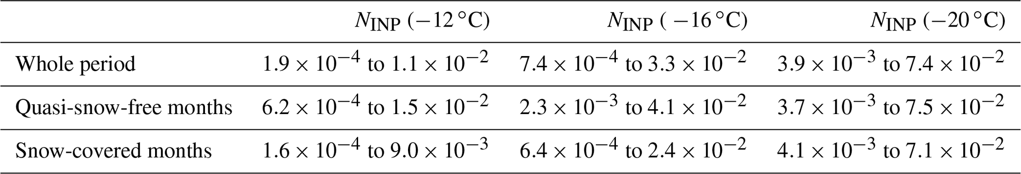
This difference in variability may be attributed to the type of aerosol particles active as INPs at the different temperatures. At −15 ^∘C or above, biological material is anticipated to act as efficient INP and to contribute to the majority of the INP population at this temperature. Local sources were proposed in the past for these INPs. It is also known that local biological processes are more pronounced in summer compared to in winter. At around −16 ^∘C and below, long-range transported INPs, most likely mineral dust, can start to show ice activity, while biological materials persist to behave as INPs and still contribute to the majority of all INPs. For temperatures below roughly −20 ^∘C, mineral dust can most likely dominate the whole INP population. This background of INPs may reduce the variation of the INP concentrations, as seen in Fig. 1 (Creamean et al., 2019; O'Sullivan et al., 2018; Kanji et al., 2017). The thermal treatment of samples points towards the existence of biological INPs at higher temperatures, which is discussed in more detail in Sect. 3.4. It should also be mentioned that the upward and downward pointing triangles in Fig. 1 indicate N_INP above and below the detectable range of the used freezing assays, respectively. The symbols were added in order to emphasize that INPs exist above or below the detection range for the respective sample. Looking at Fig. 1, it can also be seen that in April 2020, N_INP are much higher than in April 2019. To elucidate possible reasons for this difference, a case study of these 2 months is presented in Sect. 3.5.

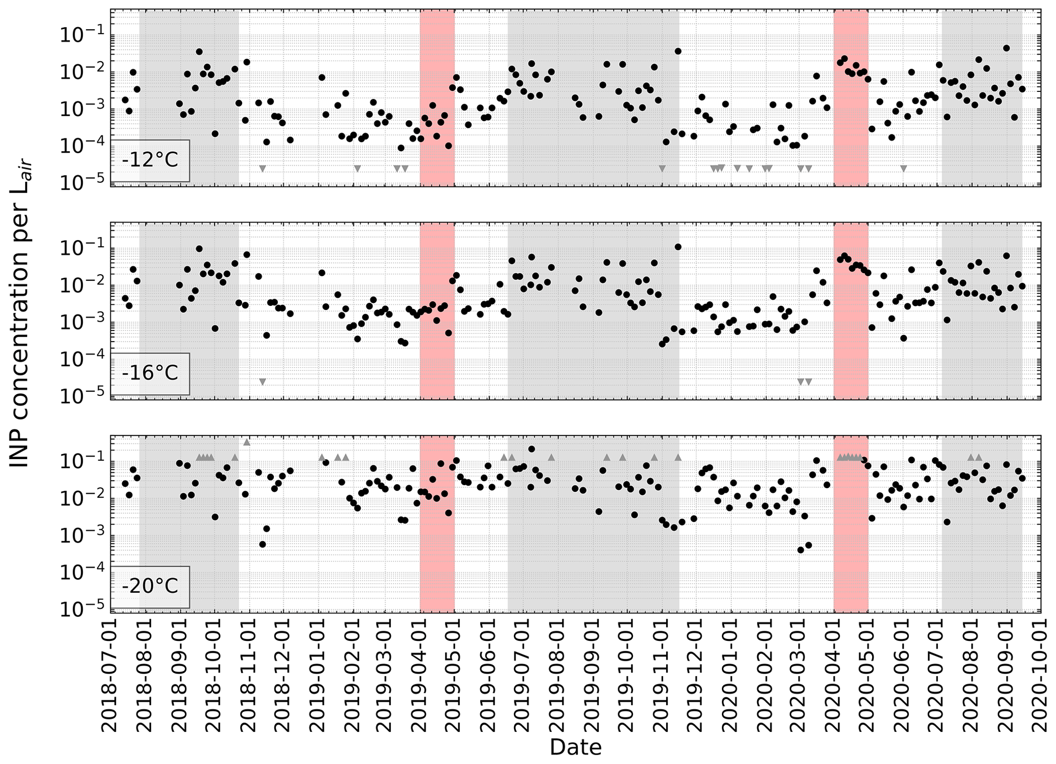
Figure 1 Time series of N_INP at −12, −16 and −20 ^∘C. Circles represent measured INP concentrations, while upward and downward pointing triangles indicate that samples have INP concentrations above or below the detectable range, respectively. Note that the detection limit varies depending on the air volume sampled on the filter. The gray areas show periods when snow depth measured at Villum Research Station (VRS) was below 0.8 m. The red areas indicate April 2019 and 2020, which are later compared in a case study.

3.2 Spectra characterization and frequency distribution of N_INP

INP spectra varied significantly throughout the 2-year-long dataset. To see if there were systematic changes, a characterization of the spectra was carried out, aiming at the division of the spectra in groups with distinct features. Just from plotting all spectra, it became obvious that they generally followed one of the three types of spectra exemplified in Fig. 2. It was particularly striking that spectra with generally lower INP concentrations were steeper, while spectra featuring higher concentrations exhibit more shallow slopes. Spectra with low concentrations generally followed a temperature (T) dependent trend roughly proportional to $e^{-\mathrm{0.6}\cdot T}$, while those with high concentrations roughly followed $e^{-\mathrm{0.3}\cdot T}$ below approximately −10 ^∘C. Those spectra in between showed shallower slopes at higher temperatures and steeper slopes at lower temperatures. The slopes in the exponential decay terms given above, −0.6 and −0.3, bring to mind those from two well-known older publications, Fletcher (1962) and Cooper (1986), respectively. Their respective INP parameterizations are often used in atmospheric models, as mentioned, e.g., in DeMott et al. (2010) and Curry and Khvorostyanov (2012). It should be noted that Fletcher (1962) reported the value of −0.6 as the usual value but commented that values between −0.4 and −0.8 were still common. In Cooper (1986), a selection of previously made measurements from literature was examined. However, it was not well described based on what criteria certain data were included or rejected. Still, when sighting this literature, it can be seen that data at higher temperatures up to −5 ^∘C were included in Cooper (1986), while Fletcher (1962) used data only downward from −10 ^∘C and mostly even below −15 ^∘C. Possibly, the presence of biological INPs active at higher temperatures, included for samples selected by Cooper (1986), but missing in the samples included in Fletcher (1962), was responsible for the differing parameterizations given in these two publications. In the present study, the reasoning behind this hypothesis will become clearer in the following.

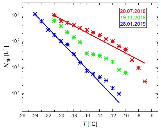
Figure 2 Three exemplary INP spectra together with fits based on exponential decay, with a slope of −0.6 for the sample with sampling end date of 28 January 2019 and −0.3 for the sample with sampling end date of 20 July 2018.

Based on the above-described observations for our own dataset, an automated discrimination of samples into three different types of spectra was aimed at. For that, each INP spectrum was fitted twice with a curve describing an exponential decay following ($A\cdot e^{s\cdot T}$). One fit was based on a fixed slope, s, of −0.6 and the second on a fixed slope of −0.3, resulting in only one free parameter, A, to be fitted. All available measured data across all temperatures, T, were included. These two slopes were chosen as they are commonly used in models, as described above, and they fit well on all of the spectra with low or high concentrations, respectively. A number of parameters resulting from these fits were examined, such as the resulting fit factors A and the root mean square differences between the measured spectra and the fits. Some parameters were clearly different between samples with high and low concentrations. The following normalized least square differences were chosen for an automated discrimination, both obtained in the temperature range between −15 and −12 ^∘C:

$$\begin{array}{}\text{(6)}& \mathrm{P}\mathrm{1}=\sum _{T=-\mathrm{15}}^{-\mathrm{12}}{\displaystyle \frac{(A{e}^{-\mathrm{0.6}\cdot T}-N_{\mathrm{INP}}{)}^{\mathrm{2}}}{(A{e}^{-\mathrm{0.6}\cdot T}{)}^{\mathrm{2}}}}\end{array}$$

and

$$\begin{array}{}\text{(7)}& \mathrm{P}\mathrm{2}=\sum _{T=-\mathrm{15}}^{-\mathrm{12}}{\displaystyle \frac{(A{e}^{-\mathrm{0.3}\cdot T}-N_{\mathrm{INP}}{)}^{\mathrm{2}}}{(A{e}^{-\mathrm{0.3}\cdot T}{)}^{\mathrm{2}}}},\end{array}$$

where P1 indicates how well the steeper slope of −0.6 describes the measured values in the temperature range from −15 to −12 ^∘C, and P2 indicates the same for the less steep slope of −0.3. Samples for which the steeper slope of −0.6 fit well in the temperature range from −15 to −12 ^∘C have a comparably low P1. All samples for which P1 $<\mathrm{5}\times {\mathrm{10}}^{-\mathrm{7}}$ were labeled as Fletcher type. The lower the relation between the two parameters $\frac{\mathrm{P}\mathrm{2}}{\mathrm{P}\mathrm{1}}$ is, the better a spectrum is described by the less steep slope of −0.3. All samples for which $\frac{\mathrm{P}\mathrm{2}}{\mathrm{P}\mathrm{1}}<\mathrm{2.5}$ were labeled as Cooper type. These were the only two criteria which were used to group the data. All remaining spectra which did not fit to one of the two criteria made up roughly 40 % of all samples. They typically had a less steep slope at temperatures above −17 ^∘C and a steeper slope below. They were labeled as mix type. An overview of the spectra of all samples color-coded according to these types are shown in Fig. S6.

Next we assessed how often each of the three spectra types occurs in each month (Fig. 3). The mix type made up roughly 40 % of all INP spectra in each month throughout the year, and roughly the remaining 60 % are almost exclusively Fletcher type in the winter months from December until March and Cooper type in the summer months from June until October. April and May as well as November are intermediate months, in which all three types of spectra occur. The results shown in Fig. 3 corroborate that the automated discrimination described above was useful to discriminate between samples typically collected in summer and winter months. Hence, hereafter, we refer to the Cooper type spectra as summer type, and to the Fletcher type spectra as winter type.

After having categorized all spectra, the frequency distributions of N_INP at each measurement temperature from −7 to −24 ^∘C for each of the three spectra types were investigated. For this, all spectra belonging to one type were combined, yielding frequency distributions of N_INP at each temperature, to which then log-normal fits were applied. This analysis was done based on Ott (1990), who suggested that log-normal distributions occur for atmospheric parameters, arising from successive random dilutions by different atmospheric processes during transportation from sources to measurement sites (as, e.g., VRS). This has been adopted for INP concentrations at different temperatures by studies such as Schrod et al. (2020), Welti et al. (2018) and recently Li et al. (2022). Figure 4 shows the frequency distributions as well as their respective log-normal fits for the same three temperatures that were selected for the N_INP time series (−12, −16 and −20 ^∘C). It can be seen that at each temperature, the distributions fitted to data from the three different spectra types cover different N_INP ranges, with the maximum of the distribution, X(T), showing the highest value for the summer type, followed by the mix type and winter type at all temperatures. Another significant feature is that with decreasing temperature the maxima of the distributions move closer together.

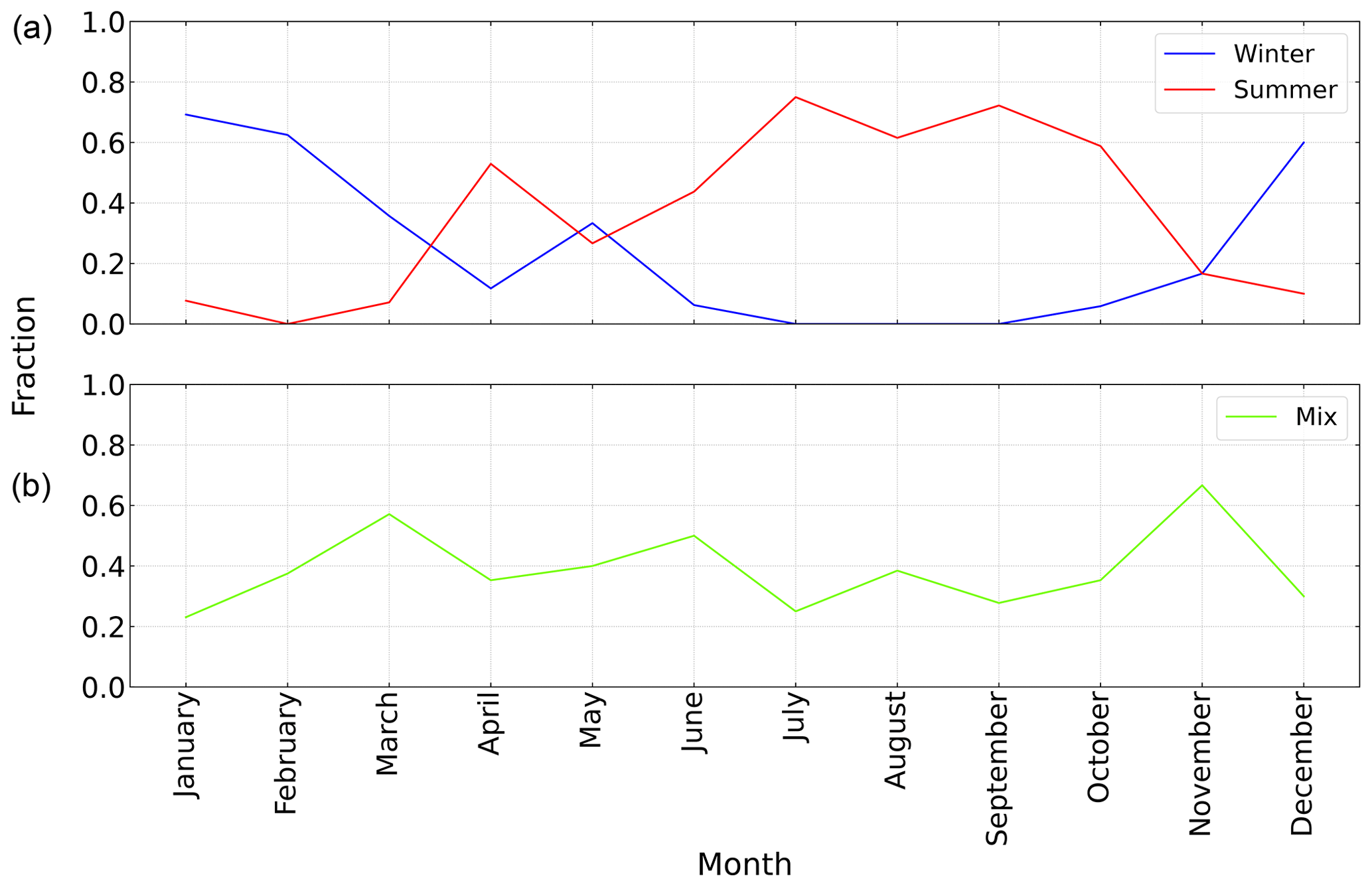
Figure 3 Time series of fractions of Fletcher type (winter) shown in blue, Cooper type (summer) shown in red, both in panel (a), and shown in light green for mix type in panel (b). Details of the number of types in each month are shown in Table S2.

As seen in Fig. 4, at −12 ^∘C, the three types show a rather distinctive distribution. Based on previous studies which found a seasonal cycle of INPs, such as Wex et al. (2019), it can be assumed that this is due to the pronounced biological activity in the ocean or on land during the summer season, while in winter, local biological processes are lacking, and long-range transported material such as mineral dust is the dominant background INP source. In mix type, neither of the two sources mentioned above is dominating, but both are contributing particles to the INP population. The transition from long-range transport to local and regional observations at Villum most likely happens in the months of April and May or may already start as early as March (Fenger et al., 2013). This explains the observation of INP spectra as mentioned above. At −16 ^∘C and further down at −20 ^∘C, the distributions of the three types get closer to each other. While biological material dominates INPs active at higher temperatures, mineral dust INPs become more noticeable and dominate the INP population when temperature gets lower. A common background of mineral dust particles throughout the year may exist (e.g., Tobo et al., 2019; Sanchez-Marroquin et al., 2020; Si et al., 2019), therefore bringing the distributions of three types closer together at lower temperatures, as seen in the lower panel in Fig. 4. In summer, when snow- and ice-covers retreat, local soil dust can be exposed to the atmosphere and contribute to the atmospheric aerosol load, contributing to the INPs population during this season.

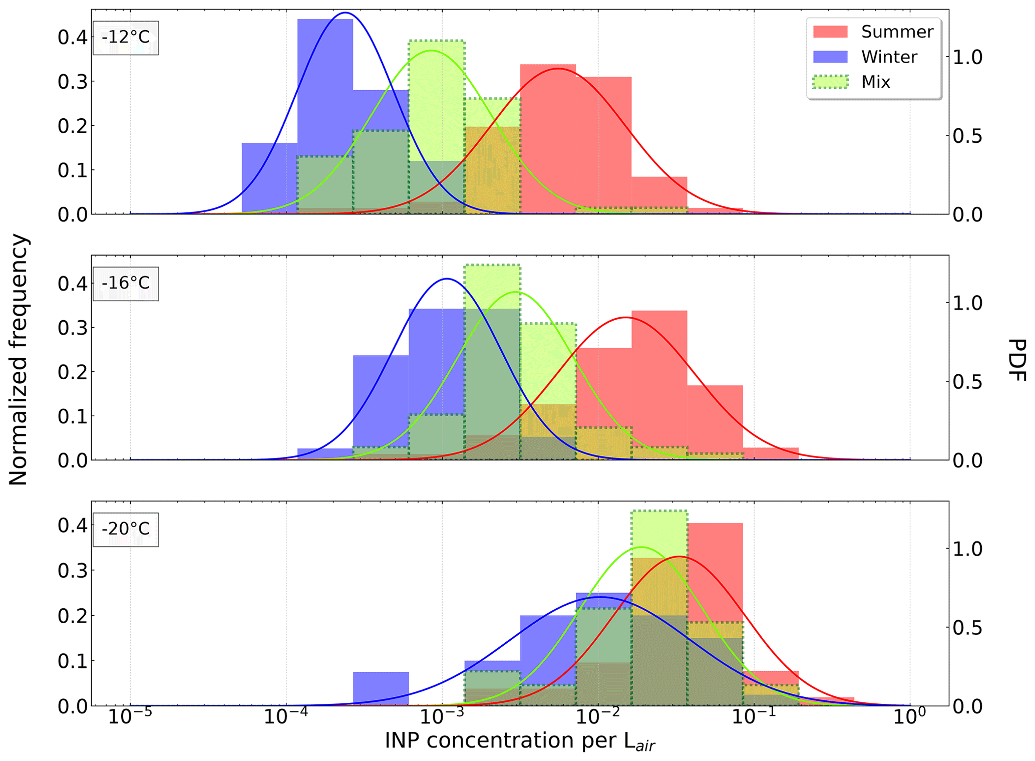
Figure 4 Normalized frequency distributions of N_INP at −12, −16 and −20 ^∘C are shown as histograms, together with corresponding log-normal fits. The axis on the right is related to the respective probability density function (PDF). The different colors represent Fletcher (winter) type in blue, Cooper (summer) type in red and mix type in light green, as described in Sect. 3.2.

3.3 Arctic INP parameterization

It was shown in recent model studies that a temperature-dependent INP parameterization is essential to accurately represent cloud properties in climate models (Hawker et al., 2021; Tan et al., 2022). In the present study, we developed three INP parameterizations, one for each of the three INP types described in Sect. 3.2. The parameterizations were derived by applying an ordinary least square (OLS) fit to the respective maximum values X(T). All resulting temperature-dependent INP parameterizations in this study follow the form of the equation below:

$$\begin{array}{}\text{(8)}& N_{\mathrm{INP}}=A\cdot e^{s\cdot T},\end{array}$$

where A and s represent the y intercept and the slope of the fit, respectively; T represents the temperature in ^∘C; and N_INP represents the atmospheric INP concentration per liter of air. Parameters of the parameterizations for summer, winter and mix type are shown in Table 2.

Table 2 Parameters of the INP parameterizations presented in this study. In addition, parameters for fits with a fixed slope are also provided for comparison purpose. The temperature ranges where the fittings were applied are also given.

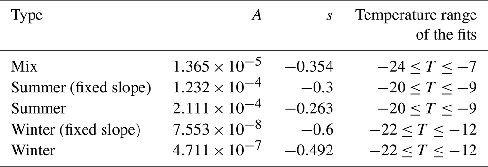
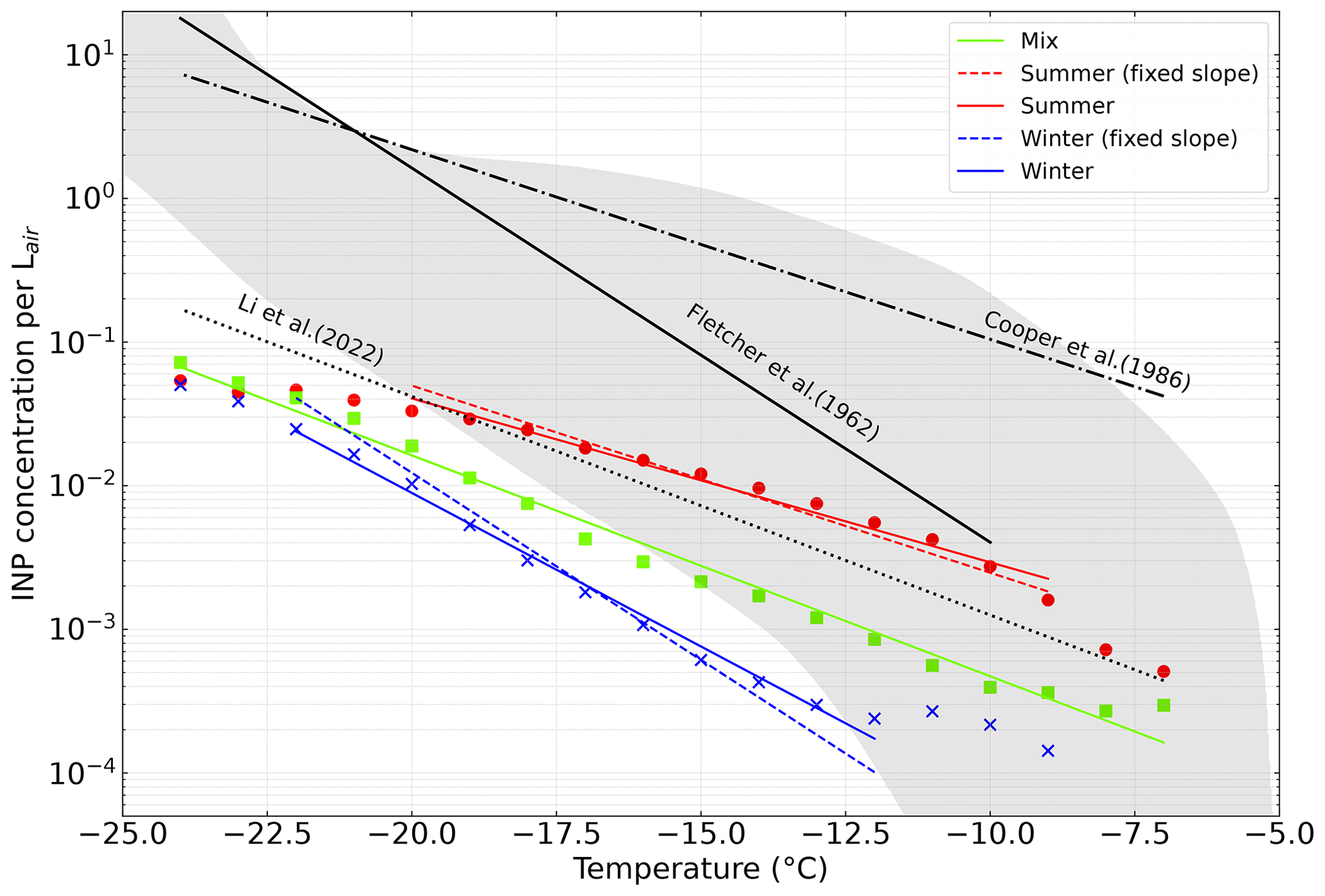
Figure 5 The INP parameterizations for summer, winter and mix type are shown as solid lines in red, blue and light green, respectively. Maxima of the log-normal fits are also shown as dots with the respective colors. For comparison the fixed slope fits (cf. Sect. 3.3) are given as dashed lines of the respective color type. For reference, also the parameterizations by Cooper (1986), Fletcher (1962) and Li et al. (2022) are shown (black lines). Also for reference, the typical range of midlatitude INP concentration according to Petters and Wright (2015) is shown as the gray-shaded area.

In addition and for comparison purposes, fitting was also conducted using Eq. (8) with fixed slope values s of −0.6 and −0.3. Respective parameters are also shown in Table 2 as reference. As discussed above, the two values of −0.6 and −0.3 for the slope originate from decades old, but still used parametrizations by Fletcher (1962) and Cooper (1986), respectively. And these are the two slopes that were at the basis of the categorization of different INP types (summer, winter and mix) used in this study (see Sect. 3.2). In Fig. 5, the parameterizations for the three different types are presented together with the maxima of the log-normal fits, X(T), at each investigated temperature. The INP parameterizations are shown as solid lines, while the fixed slope fits are shown as dashed lines. Parameterizations from Cooper (1986), Fletcher (1962) and Li et al. (2022) were also plotted for comparison. All parameterizations in this study predict INP concentration up to 3 orders of magnitude lower than Cooper (1986) and Fletcher (1962), which were not based on Arctic data. Similar to the case of the slopes, for which a broad range of values was given by Fletcher (1962) (see Sect. 3.2), Fletcher (1962) gave 10⁻⁵ L⁻¹ as the typical value for A, but also explicitly pointed towards variations for A of several orders of magnitude between the datasets used (originating from a range of cloud chambers applied in a number of atmospheric studies). Therefore, the comparison to these older parameterizations should not be overrated. The parameterization from Li et al. (2022) compares very well with the parameterization suggested for the mix type in our study, with both sharing a very similar slope and the concentration of the latter being only a factor of ≈3 lower. This is not surprising, as the parameterization by Li et al. (2022) was derived from measurements taking place in October and November 2019 and in March and April 2020, but further south on Svalbard. These months largely overlap with those that were found to be dominated by the mix type in our study (November) or not having a clearly dominating type (April and May), which clearly highlights the need to carry out long-term measurements as done in the present paper in order to get the right understanding of the dynamics and processes of environmental parameters such as INPs. An overview of the frequency distributions of N_INP at the investigated temperature range, along with the suggested INP parameterizations, are shown in Fig. 6. The median, 25th and 75th percentile of each distribution are shown as solid and dashed lines. As expected, it can be seen that N_INP distributions feature an increasing trend with lowering temperatures. In general, summer type distributions show a higher median compared to the mix type, while distributions of the winter type show a lower median compared to the mix type. This is consistent with what is shown in Fig. 4. We furthermore examined which fraction of the corresponding samples falls within a range covering one order of magnitude above and below our parameterizations. This fraction is generally well above 90 %, as shown at three selected temperatures of −12, −16 and −20 ^∘C in Table 3 (for more details see Fig. S7), emphasizing the representativeness of our parameterizations.

As described in Sect. 3.2, winter, summer and mix type show different fractions of occurrence throughout the year, varying depending on the month but with the summer and winter type dominating the summer and winter months, respectively. In order to strategically implement the parameterizations from this study into climate and cloud-resolving models, the authors propose the following strongly simplified scheme:

• winter type, to be used 60 % of the time from December to March and 30 % of the time in April, May and November:
  $N_{\mathrm{INP}}\left(T\right)=\mathrm{4.711}\times {\mathrm{10}}^{-\mathrm{7}}\times e^{-\mathrm{0.492}\cdot T}$;

• summer type, to be used 60 % of the time from June to October and 30 % of the time in April, May and November:
  $N_{\mathrm{INP}}\left(T\right)=\mathrm{2.111}\times {\mathrm{10}}^{-\mathrm{4}}\times e^{-\mathrm{0.263}\cdot T}$;

• mix type, to be used 40 % of the time throughout the year:
  $N_{\mathrm{INP}}\left(T\right)=\mathrm{1.365}\times {\mathrm{10}}^{-\mathrm{5}}\times e^{-\mathrm{0.354}\cdot T}$.

This is only a rough representation, and if favored, more highly resolved monthly values can be taken from Fig. 3. Overall, these results clearly show that differing parameterizations, depending on the time of year, are needed to describe INPs in the Arctic. However, three different base cases, as those derived above, may suffice.

Table 3 Fraction of samples (in %) falling in the range of a factor of 10 above to a factor of 10 below the parameterizations given in Table 2 for $T=-\mathrm{12}$, −16 and −20 ^∘C (for all spectra together with the parameterizations and upper and lower bounds, see Fig. S7).

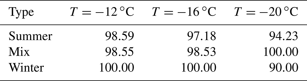
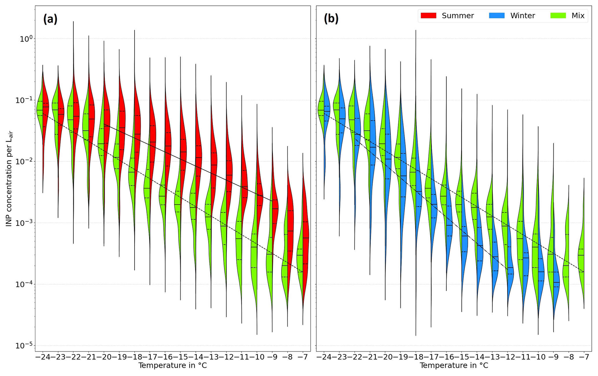
Figure 6 Violin plots of the N_INP(T) frequency distribution from −7 to −24 ^∘C, given in the typical color used for the corresponding types (a: summer type; b: winter type; both panels: mix type, shown in both panels for reference). For the distributions, solid horizontal lines show the median, and dashed horizontal lines show the 25th and 75th percentile, respectively. The parameterizations suggested in this study are also plotted as a solid black line (summer) in panel (a), a dash–dot black line (winter) in panel (b) and a dashed black line (mix) in both panels.

3.4 Heat-labile ratio and thermally treated samples

Thermal treatment of the samples showed that the ice activity for most of the samples was reduced after heating for 1 h at 85 ^∘C or 90 ^∘C. The heat-labile ratio, which is used to represent the fraction of heat-labile INPs in each sample, was evaluated by using Eq. (5), as described in Sect. 2.2.7. A time series of the heat-labile ratio at −12, −16 and −20 ^∘C is shown in Fig. 7 (similarly, Fig. S8 shows the time series of fractions of heat-labile INPs at three additional temperatures and also color-coded according to the different types). A seasonal cycle is again observed at −12 and −16 ^∘C. In general, a higher fraction of heat-labile INPs was found in samples collected during the quasi-snow-free months than during months with a snow cover. It is also worth mentioning that even in snow-covered months, at −12 ^∘C, a heat-labile ratio fraction of 0.75 or higher can be reached. At −16 ^∘C, the heat-labile ratios in both quasi-snow-free and snow-covered months are generally lower than at −12 ^∘C. At −20 ^∘C, not enough data points exist to provide an insight on the fraction of heat-labile material.

Based on the categorization described before (i.e., winter, summer and mix type), the heat-labile ratio of samples separating into these types was examined as well. Box plots of these three types are shown in Fig. 8. Summer type in general shows the highest heat-labile ratio, while winter type shows the lowest. Mix type shows a heat-labile ratio in-between the summer and winter type. This corroborates the interpretation in Sect. 3.2 that summer type is indeed most likely dominated by biological INPs, with heat-labile ratios often above 0.8, particularly above −15 ^∘C. Although the number of background INPs cannot be directly interpreted through the heat-labile ratio plot, the relatively low number of heat-labile INPs in the winter type (compared with summer and mix type) indicates that roughly at least half of all INPs during that period were comprised of non-proteinaceous biological material. The atmospherically most abundant non-biological INPs are mineral dust particles. And as local Arctic sources are sparse in winter, due to the surface being covered in snow and ice, it is likely that the observed background INPs originate from long-range transport. All three types feature a decreasing heat-labile ratio with decreasing temperature, indicating that an increasing fraction of all INPs is contributed by background mineral dust towards lower temperatures. This is in line with the observation presented in Fig. 4, where the distributions of the three types converged at lower temperatures.

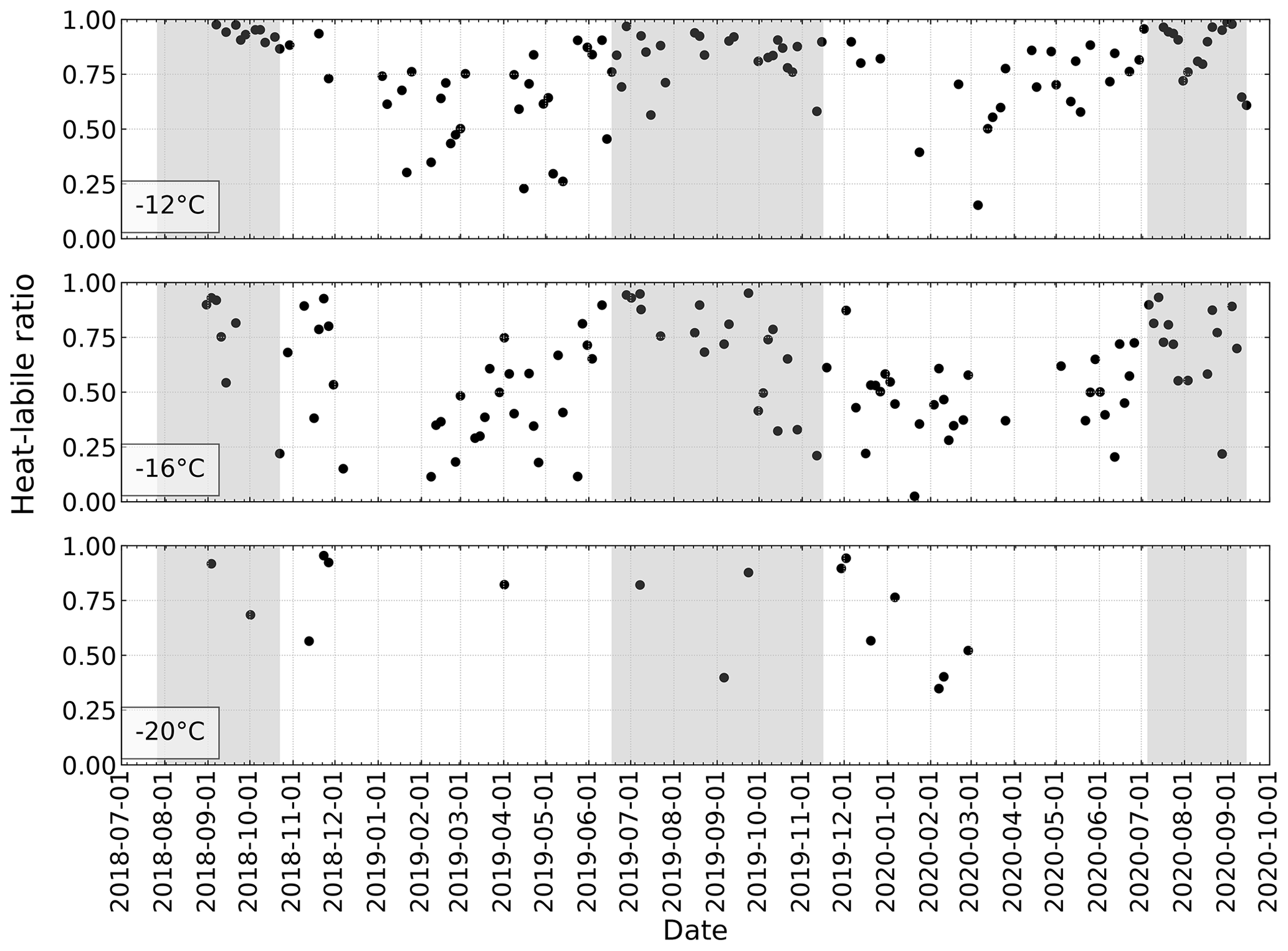
Figure 7 Time series of the heat-labile ratio at −12, −16 and −20 ^∘C. The gray area indicates the time period with a snow depth below 0.8 m.

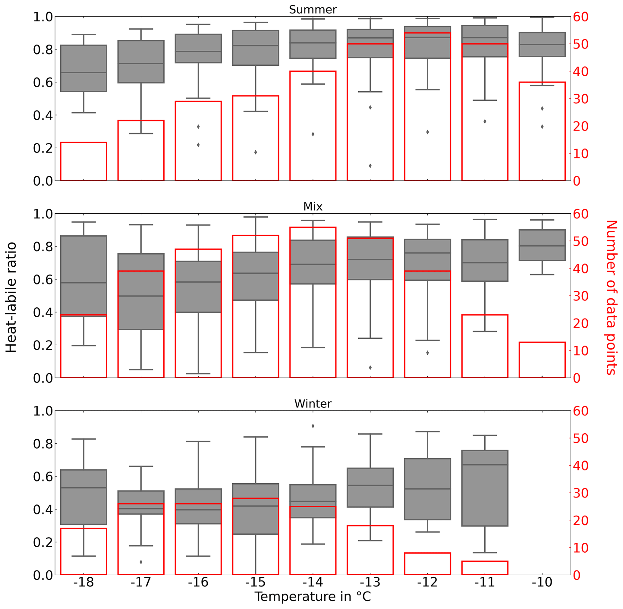
Figure 8 Box plots of the heat-labile ratio for summer, mix and winter type from −10 to −18 ^∘C. Bar plots (in red) show the number of data points at each temperature.

3.5 Case study

As seen in Fig. 1, N_INP in April 2020 was noticeably higher compared to the same month in 2019. To further investigate the cause of the differences, 5 d back trajectories were used to determine the origin of the sampled air masses. In Fig. 9, examples are given for one filter collected in 2019 and one collected in 2020. Trajectories arriving at 50 m are shown for locations where they were at heights below 250 m (in red). The trajectories are overlaid on the sea-ice concentration map for the sampling period of the filters, which were sampled for 3.5 d prior to 1 April 2019 and 10 April 2020, respectively. Maps for all other filters collected in April 2019 and 2020 can be found in Figs. S9 and S10. The altitude threshold of 250 m above ground was applied in order to locate potential source regions within the planetary boundary layer. It can be seen in Fig. 9 that for both filters the air masses arriving at VRS were only below 250 m in proximity to coastal areas of Greenland. Near the coast, both local marine and terrestrial sources can potentially contribute to the INP population.

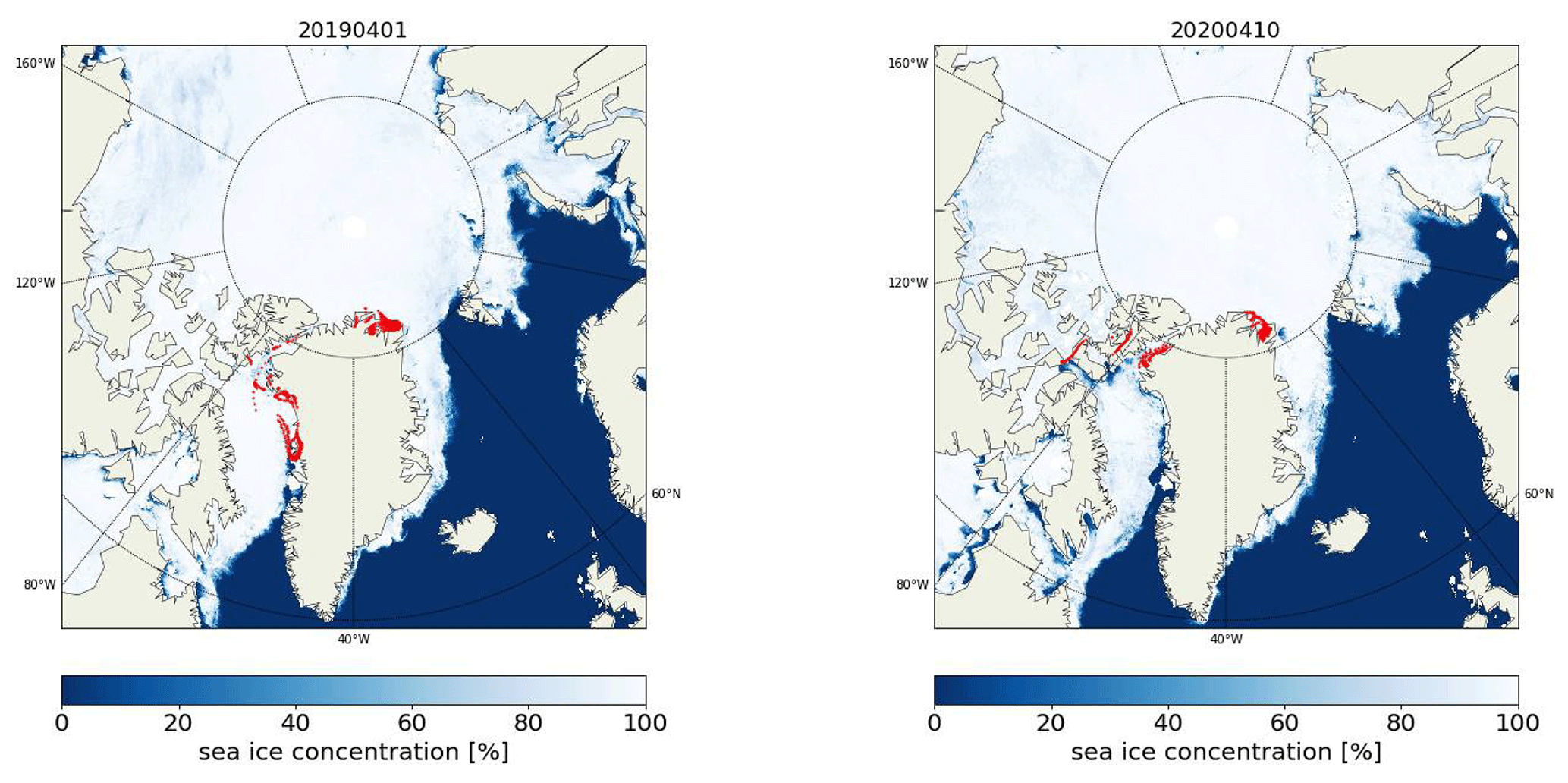
Figure 9 Shown in red are 5 d back trajectories (50 m a.g.l. arrival height at VRS) for times when they were below 250 m. The two panels correspond to sampling times of two filters, for which the sampling end dates were 1 April 2019 and 10 April 2020. Averaged sea-ice concentrations during the sampling periods are also presented.

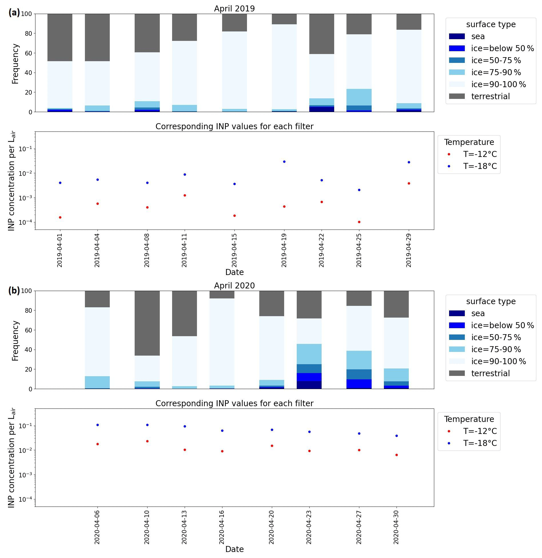
Figure 10 Frequency of the occurrence of different surface types below the trajectory for the sampling period of each filter collected in April 2019 (a; upper panel) and April 2020 (b; upper panel) are shown as stacked bar plots. Their corresponding INP concentrations at −12 and −18 ^∘C are shown in lower panels of (a) and (b) as references. Data points are drawn at the end date of the sampling period of each of the 3.5 d filters.

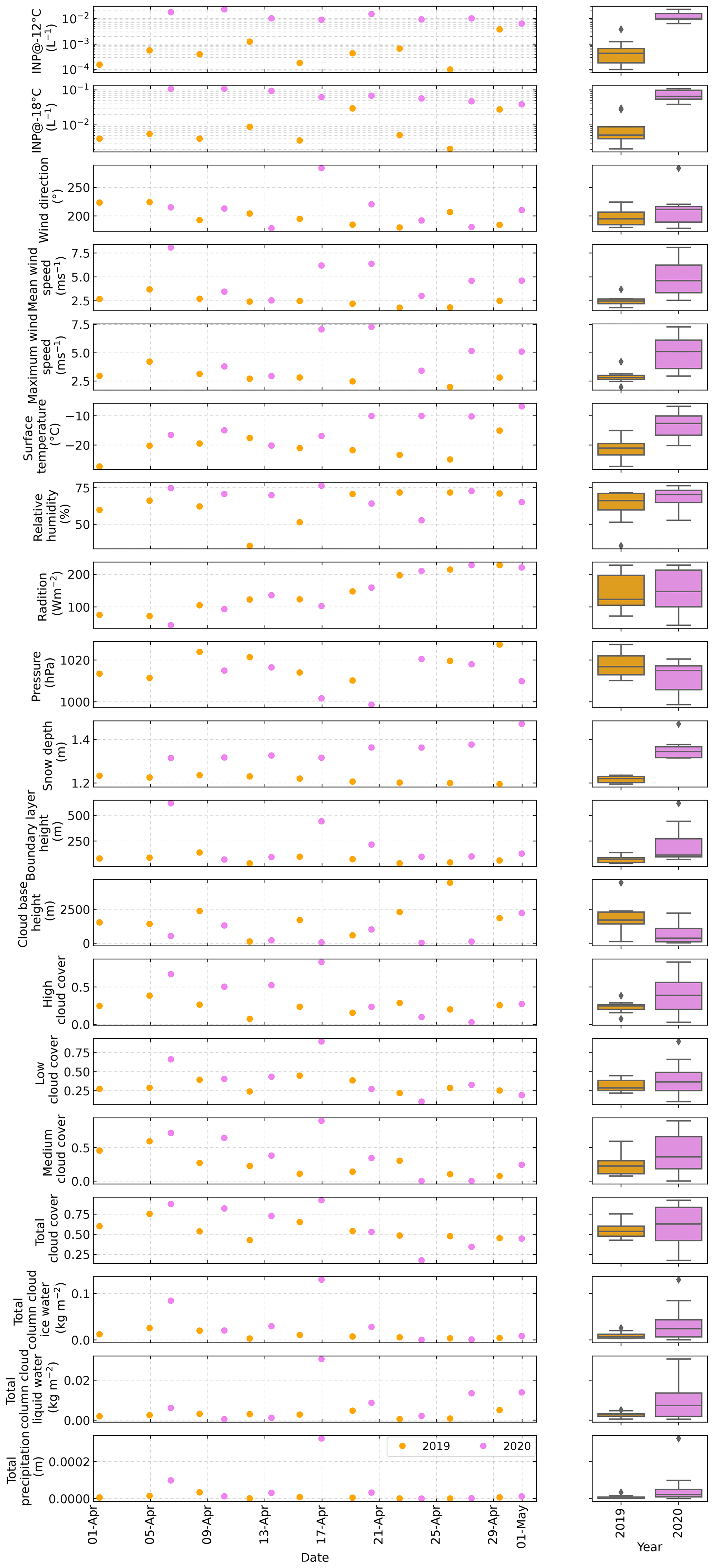
Figure 11 Filter-wise average of investigated meteorological parameters as well as the INP concentration at −12 ^∘C and −18 ^∘C in April 2019 (orange) and 2020 (purple) are shown in time series (left). Corresponding box plots of all data points in the April of the respective year are shown on the right hand panel.

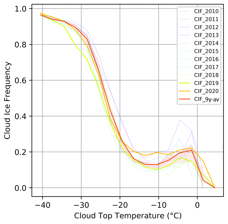
Figure 12 Temperature-dependent CIFs at the latitude band between 75 and 85^∘ N for the years 2010 to 2020, and the average for 2010–2018 (with the shaded area covering the 25th to 75th percentile).

The same 5 d back trajectories were used further to quantitatively investigate the difference of INP sources between April 2019 and 2020. For that, the number of time trajectories spent above different surface types at altitudes below 250 m was evaluated for each sample collected during the 2 months and expressed in frequency in Fig. 10. The surface was categorized into the following types: terrestrial, open sea, sea-ice concentration (<50 %), sea-ice concentration (50 %–75 %), sea-ice concentration (75 %–90 %) and sea-ice concentration (90 %–100 %). In both years sea ice with concentrations above 90 % contributed the most to the air masses sampled for most of the filters, with some occasions when terrestrial surfaces and sea ice with lower concentration played a larger role. Values for these frequencies are shown in Tables S3 and S4, respectively. This back-trajectory analysis shows no obvious difference in the air mass history between the two years. Satellite remote sensing products show that along the coastal areas in the investigated region patches of low sea-ice concentration and low snow cover exist. However, a more small-scale attribution of the air mass to these possible marine or terrestrial source regions is not meaningful when the accuracy of the back trajectories and the satellite products is considered.

Further efforts were made by investigating the relation between the INP concentration and a broad range of available meteorological parameters, as mentioned in Sect. 2.2.8 and shown in Fig. 11. The values shown in the time series in Fig. 11 were averaged over the sampling period of each filter, and the right hand panels show a box plot each for all data points in 2019 and 2020. No significant dependence of INP concentration on meteorological parameters was observed in these 2 years. This can also be seen in the correlation plots in Figs. S11 and S12. Nor was there a difference between the 2 years which could meaningfully explain the difference in INP concentrations. Nevertheless, we highlight the following observations: the snow depth in 2020 was constantly above that in 2019, but they were, however, above 1 m at all times; maximum and mean wind speed and the surface temperature were all higher in the second half of the month in 2020 compared to in 2019. However, INP concentrations were elevated throughout all of April 2020. These higher values in the second half of April 2020 were likely connected to a warm air mass intrusion as observed on the research vessel Polarstern (Dada et al., 2022), which was roughly located at 84.6^∘ N, 14^∘ E, about 800 km northeast of VRS. This intrusion observed at Polarstern from 14 to 16 April likely connected to the higher temperatures and wind speeds observed at VRS in the second half of April. But again, this cannot explain the elevated INP concentrations observed throughout April 2020. We also want to point out that blowing snow occurring in the Arctic (Yang et al., 2019) may contribute to atmospheric INP. However, in our case, due to the use of a PM₁₀ inlet during filter sampling, we do not expect that snow was collected in considerable amounts, and hence we do not expect an influence of blowing snow on our measured INP concentrations.

In a further effort, we examined if the increased INP concentrations in April 2020 correlated with the frequency of occurrence of ice in clouds, for which we obtained the CIF (cloud-ice frequency) from satellite data. In Fig. 12, temperature-dependent CIFs for the 75–85^∘ latitude band are shown for the months of April for altogether 11 years, from 2010 to 2020, together with an average curve for the years 2010–2018. For temperatures above −20 ^∘C, CIF for 2020 was above CIF for 2019 as well as above the average from 2010–2018. Figure 13 shows, that the effect of higher CIF in 2020 was indeed present in all of the latitudinal band above 80^∘ and was particularly pronounced in northern Greenland. Therefore, the higher INP concentrations observed at the surface may have caused a larger cloud-ice content, which, in turn, may have influenced cloud-radiative properties and precipitation formation and in turn cloud lifetime, resulting in an influence on surface temperatures. Also, the increasing snow depth during April 2020 may result from stronger precipitation formation. While this is all speculative, the observed higher CIF in 2020 is clearly in line with the observed higher INP concentrations.

Overall, INP concentrations show no correlation between examined surface types and meteorological parameters. Efforts of correlating the INP concentration in the Arctic with aerosol physical properties such as aerosol concentration, fluorescent particle concentration and particle surface concentration were made in connection with a recent study by Li et al. (2022), in which no relationship between INP concentrations and the above-mentioned parameters was found. This altogether illustrates the difficulties in predicting INP concentrations based on INP sources, on meteorological parameters or on aerosol properties. Instead, as already argued in Li et al. (2022), simple parameterizations, yielding temperature-dependent INP concentrations, seem beneficial, with the constraint that these may differ by season as the ones derived in this study.

4 Summary and conclusions

Results from 2-year-long INP measurements at Villum Research Station located in northern Greenland have been presented in this study. Filter samples were collected on a half-weekly basis from July 2018 to September 2020. Offline INP droplet freezing arrays were used to analyze the INP concentration, N_INP(T), in the temperature range relevant for mixed-phase clouds. A seasonal cycle of N_INP was observed at higher temperatures, exemplarily presented at −12 and −16 ^∘C. Quasi-snow-free months featured clearly higher N_INP compared to months when the surface was snow-covered. This finding aligns with previous literature, such as Šantl Temkiv et al. (2019), Wex et al. (2019) and Creamean et al. (2018), describing higher INP concentrations during summer compared to winter. Heating tests were performed in order to assess the fraction of heat-labile INPs (likely proteinaceous, of biogenic origin) in relation to the total number of INPs (referred to as heat-labile ratio). A seasonal cycle was again observed for the heat-labile ratio at temperatures above −16 ^∘C. Nonetheless, even during months with surface snow cover, heat-labile ratios at −12 ^∘C can be as high as 0.75 and sometimes even larger. Still, the higher heat-labile ratio in the quasi-snow-free months shows that an annual cycle of N_INP mostly occurs due to the seasonality of biological sources throughout the year. The whole dataset was categorized based on the slope of the respective INP spectra, resulting in three types of spectra, namely summer, winter, and mix type. For these three types, the frequency distribution of N_INP was derived and fitted with log-normal distributions for different temperatures. At higher temperatures (e.g., −12 ^∘C) the maxima of the fitted distributions are clearly different from each other, while with decreasing temperatures the differences between the distributions become less and less pronounced. This shows that at high temperatures distinct INP populations with different ice-nucleation efficiencies are present, while at low temperatures only an almost uniform INP population seems to exist. This, together with the finding that the heat-labile ratio shows a decreasing number of heat-labile INPs with decreasing temperature is interpreted as follows: highly ice-active biological INPs are the cause for high INP concentrations at high temperatures (roughly −16 ^∘C and above). These highly efficient INPs occur additionally to a more generally present and less efficient background INP population. With decreasing temperatures the biological INPs become less prominent, until they blend with the background INP population at the lower temperatures (−20 ^∘C and below). A temperature-dependent INP parameterization based on mean INP concentrations from log-normal fits, done at different temperatures, was derived for each of the aforementioned types (winter, summer and mix). While the summer type INP spectra occurred during 60 % of all times in the summer months and the winter type during 60 % of all times during the winter months, the mix type occurred 40 % of all times year-round, and April, May and November were transition months. With this information, these parameterizations can be easily implemented into climate and cloud-resolving models, because they only depend on temperature and the month of the year in order to deliver a prediction of N_INP(T) in the high Arctic throughout the year. This will improve the description of the annual cycle of INP concentrations as observed in the Arctic for modeling purposes.

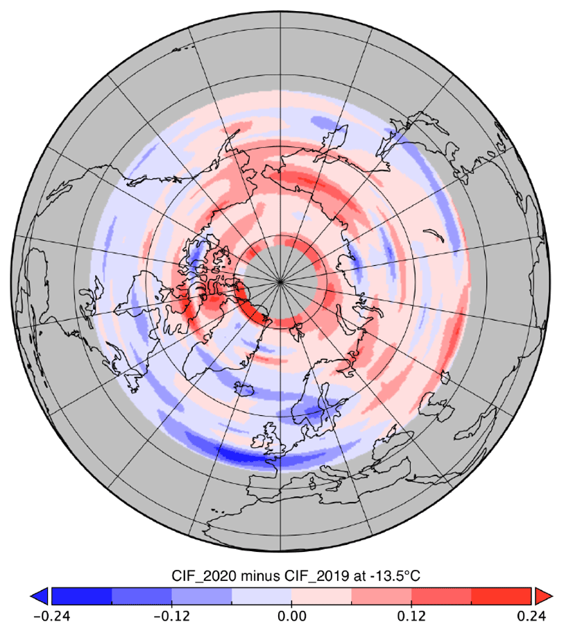
Figure 13 CIF during April 2020 minus CIF during April 2019 at a cloud top temperature of −13.5 ^∘C (only data above 45^∘ N are shown).

A case study investigating possible causes for significant differences in N_INP found between April 2019 and 2020 was carried out. Back trajectories indicate that the sampled air masses mainly originated from coastal regions of Greenland in both years. Therefore, both local terrestrial and marine sources could potentially contribute to the collected INPs. INP concentration shows no dependency on different surface types and meteorological parameters in these two periods, and no parameter was found which was clearly different in April 2019 and April 2020. However, examining satellite data, we found a higher cloud-ice fraction for the year with higher INP concentrations, suggesting a possible link between INP concentration and ice in clouds. Altogether the results of our investigations indicate the complexity of predicting Arctic INP and their effects on clouds. It further emphasizes the need for suitable models from the large eddy simulation (LES) to global scales, and the importance of using appropriate, e.g., solely temperature based, parameterizations therein.