Turbulent structure of the Arctic boundary layer in early summer driven by stability, wind shear and cloud-top radiative cooling: ACLOUD airborne observations

Clouds are assumed to play an important role in the Arctic amplification process. This motivated a detailed investigation of cloud processes, including radiative and turbulent fluxes. Data from the aircraft campaign ACLOUD were analyzed with a focus on the mean and turbulent structure of the cloudy boundary layer over the Fram Strait marginal sea ice zone in late spring and early summer 2017. Vertical profiles of turbulence moments are presented from contrasting atmospheric boundary layers (ABLs) from 4 d. They differ by the magnitude of wind speed, boundary-layer height, stability, the strength of the cloud-top radiative cooling and the number of cloud layers. Turbulence statistics up to third-order moments are presented, which were obtained from horizontal-level flights and from slanted profiles. It is shown that both of these flight patterns complement each other and form a data set that resolves the vertical structure of the ABL turbulence well. The comparison of the 4 d shows that especially during weak wind, even in shallow Arctic ABLs with mixing ratios below 3 g kg⁻¹, cloud-top cooling can serve as a main source of turbulent kinetic energy (TKE). Well-mixed ABLs are generated where TKE is increased and vertical velocity variance shows pronounced maxima in the cloud layer. Negative vertical velocity skewness points then to upside-down convection. Turbulent heat fluxes are directed upward in the cloud layer as a result of cold downdrafts. In two cases with single-layer stratocumulus, turbulent transport of heat flux and of temperature variance are both negative in the cloud layer, suggesting an important role of large eddies. In contrast, in a case with weak cloud-top cooling, these quantities are positive in the ABL due to the heating from the surface.

Based on observations and results of a mixed-layer model it is shown that the maxima of turbulent fluxes are, however, smaller than the jump of the net terrestrial radiation flux across the upper part of a cloud due to the (i) shallowness of the mixed layer and (ii) the presence of a downward entrainment heat flux. The mixed-layer model also shows that the buoyancy production of TKE is substantially smaller in stratocumulus over the Arctic sea ice compared to subtropics due to a smaller surface moisture flux and smaller decrease in specific humidity (or even humidity inversions) right above the cloud top.

In a case of strong wind, wind shear shapes the ABL turbulent structure, especially over rough sea ice, despite the presence of a strong cloud-top cooling. In the presence of mid-level clouds, cloud-top radiative cooling and thus also TKE in the lowermost cloud layer are strongly reduced, and the ABL turbulent structure becomes governed by stability, i.e., by the surface–air temperature difference and wind speed. A comparison of slightly unstable and weakly stable cases shows a strong reduction of TKE due to increased stability even though the absolute value of wind speed was similar. In summary, the presented study documents vertical profiles of the ABL turbulence with a high resolution in a wide range of conditions. It can serve as a basis for turbulence closure evaluation and process studies in Arctic clouds.

1 Introduction

Within the past 2 decades an extraordinary climate change has been observed in the Arctic. Numerous processes and feedback mechanisms have been proposed and discussed as possible reasons for the currently ongoing changes resulting in an enhanced Arctic warming compared to the mid-latitudes, which is generally called the Arctic amplification. The effect of the processes and feedbacks has been well documented by a large number of modeling and observational studies (e.g., Serreze and Francis, 2006; Graversen et al., 2008; Overland et al., 2011; Wendisch et al., 2017; Osborne et al., 2018). While the changes are obvious, the chain of interlinked processes and complex air–sea-ice–ocean interactions leading, e.g., to reduced sea ice cover is not yet fully explored and quantified. One of the key factors in the framework of Arctic amplification feedbacks is clouds and their various effects, which are in the center of this work. In early studies (e.g., Curry et al., 1996; Morrison et al., 2011; Shupe et al., 2011) it was found that low-level stratocumulus clouds frequently occur over the Arctic and influence the surface heat budget and consequently the sea ice mass budget. In more recent investigations, clouds have been recognized to be involved in different feedback mechanisms contributing to the observed warming (e.g., Serreze and Francis, 2006; Pithan and Mauritsen, 2014; Goosse et al., 2018; Stapf et al., 2020). However, despite the progress, there are still gaps in knowledge related to the quantification of the role of specific processes affecting cloud properties over sea ice.

One of the difficulties is the complex interaction of processes of different physical nature and scale, such as radiation, turbulence and cloud microphysics, as well as their interplay with large-scale synoptic forcing and variable surface conditions (e.g., Curry et al., 1996). In particular, interactions with turbulence, as well as the turbulent exchange with the surface and overlying air, have a strong impact on clouds (Morrison et al., 2011). Low-level clouds often reside in the atmospheric boundary layer (ABL) and thus affect its properties and the energy exchange with sea ice. However, cloud layers are also frequently decoupled from the surface-based atmospheric boundary layer (e.g., Curry, 1986). Both the treatment of clouds and the ABL over Arctic sea ice remain weak points of modern atmospheric models (Tjernström et al., 2005, 2008; Pithan et al., 2014). Therefore, further research focused on a combined consideration of cloud, radiation and turbulence properties is needed.

Although the crucial effects of Arctic clouds on the ABL energetics and turbulence structure are widely accepted, a quantification, especially over sea ice covered regions, is difficult since data are available from only a limited number of campaigns. Mixed-phase clouds represent one of the most complex challenges (e.g., Morrison et al., 2011). They occur most frequently in the cold seasons but also during early summer, which is considered in this work. The first analyses of the impact of summer Arctic boundary-layer clouds on the turbulent structure and on ABL energy fluxes using in situ aircraft observations were presented by Curry (1986) and Curry et al. (1988) based on a data set obtained more than 4 decades ago. The detailed analysis offers insight into the combined effect of radiation and turbulence, but findings are based on only four cases with very limited vertical resolution for turbulence measurements. Only three more cases were documented later, namely by Finger and Wendling (1990), Brümmer et al. (1994) and Inoue et al. (2005), providing additional yet still insufficient data for process understanding and model evaluation.

These studies have shown that the main effect of clouds is associated with radiative cooling at the cloud top. In particular, the latter leads to convective overturning and generation of turbulence due to buoyancy. This process is well-known for stratocumulus in lower latitudes. As stressed by Curry et al. (1988), Arctic clouds occur frequently in multiple layers. In such cases, the strongest radiative cooling as well as the buoyancy production of turbulence occurs in the uppermost cloud layer, which is far from the surface and thus decoupled. In the lowest, surface-based layer, which is often stably stratified, wind shear becomes the main mechanism of turbulence generation (Inoue et al., 2005). These findings were confirmed using a large data set obtained from surface-based cloud radar during the Arctic Summer Cloud Ocean Study (ASCOS, Shupe et al., 2013; Tjernström et al., 2014; Sedlar and Shupe, 2014; Sotiropoulou et al., 2014).

However, due to the very limited number of in situ observations, gaps remain in a large region of the parameter space. Namely, except from the ASCOS cases, the mentioned studies presented cases with a rather strong wind speed (10 m s⁻¹ and stronger). Thus, weak to moderate wind speed conditions still remain uncovered by observations. Also, the multi-layer cases, studied earlier, were characterized exclusively by negative heat fluxes in the surface-based boundary layer. To conclude, the effect of a variable wind shear and stability on the turbulent structure of a cloud-topped ABL and on the cloud properties cannot be well assessed based on these studies alone.

One of the goals of this paper is therefore to extend the earlier data sets by turbulence data obtained for another four cases from the airborne measurements during polar day (ACLOUD) campaign (Wendisch et al., 2019). After that, the available data base is still small but it is another step forward, which helps to reach the second goal, namely to gain a better understanding of processes affecting the turbulent structure of the Arctic ABL in the presence of clouds. The data will be used to describe and analyze the mean and turbulent structure of the cloudy boundary layer in terms of turbulent and radiative energy quantities over sea ice found in early summer. The ACLOUD campaign was carried out in May–June 2017 over the Fram Strait marginal sea ice zone (MIZ) to the northwest from Svalbard. Unlike in most previous studies, we consider not only the more qualitative turbulence structure (as possible by surface-based radar measurements) but quantify also the fluxes of momentum, heat and radiative energy as well as further turbulence quantities such as turbulent kinetic energy, variances and higher-order turbulence moments. Compared with Finger and Wendling (1990), a new aspect is to consider the variability due to the impact of external factors such as the mean wind field and multi-layer clouds and to obtain a better vertical resolution. The latter is also an advantage compared with the studies of Curry (1986) and Curry et al. (1988).

Our strategy is – as to some extent also in the study of Curry (1986) – to investigate several contrasting cases with low-level clouds highlighting the forcing mechanisms of turbulence and their variability. One of the important forcing parameters is the strength of mean wind, which varies from case to case due to a different synoptic situation. Second, we will show that the intensity of the cloud-top radiative cooling and thus of turbulence is strongly modulated by the presence of multi-layer clouds. This extends the above-mentioned study of Inoue et al. (2005) on the effect of a two-layer cloud system. Third, we document how surface roughness and wind direction modulate stratification and turbulence parameters in a cloudy boundary layer and in turn the ABL height and cloud thickness. We will discuss similarities and differences to earlier findings using the new data set, which will help to better understand the most important features in Arctic boundary-layer clouds.

The paper is structured as follows. We introduce the campaign and describe the measurement equipment in Sect. 2. Results of different flights are presented in Sect. 3. A final discussion and conclusions follow in Sects. 4 and 5, respectively. Appendix A contains information concerning the accuracy of the measurements, Appendix B presents vertical profiles of net terrestrial radiative flux densities and associated cooling rates, and Appendix C describes a diagnostic mixed-layer model addressed in Sect. 4.

2 ACLOUD campaign

During the ACLOUD campaign the two research aircraft Polar 5 and Polar 6 (Wesche et al., 2016) of the German Alfred Wegener Institute were used for collocated measurements in the cloudy and cloud-free atmospheric boundary layer (ABL) over the open ocean and the marginal sea ice zone to the north and west of Svalbard. The general strategy was to use Polar 5 as a remote-sensing platform for cloud observations from above and Polar 6 for in situ measurements in clouds and below them (Wendisch et al., 2019). During some flights both aircraft were used for in situ observations.

ACLOUD took place during May and June 2017, covering the transition from late spring to early summer meteorological conditions at the end of May (Knudsen et al., 2018). During the first two weeks of June 2017, several episodes with warm air advection took place so that the air temperature increased over sea ice but it still remained below zero. The majority of flights above, in and below low-level stratocumulus clouds over sea ice and open ocean were performed during this period.

During the ACLOUD period the research vessel (RV) Polarstern (PS) of the Alfred Wegener Institute was drifting in the sea ice north of Svalbard (Wendisch et al., 2019). Some flights were carried out next to the ship but, e.g., safety rules did not allow parallel measurements in clouds with the tethered balloon (Egerer et al., 2019), which was operated next to the ship.

2.1 Aircraft instrumentation and data processing

The instrumentation of both aircraft including radiation and turbulence equipment is overviewed in Wendisch et al. (2019) and in Ehrlich et al. (2019). Here, we only summarize the relevant information about the instrumentation for turbulence and boundary-layer observations. For measurement uncertainty we refer to Hartmann et al. (2018) and to further aspects described in Appendix A.

Both aircraft were equipped with identical meteorological instrumentation mounted at the nosebooms. It includes the Rosemount 858 five-hole probes and two fast-response open-wire Pt100 temperature sensors in deiced and non-deiced Rosemount housings. Each aircraft was also instrumented with slow-response Vaisala temperature and humidity sensors (HMT-333) and also with static pressure sensors. Downward and upward shortwave and terrestrial longwave radiative energy fluxes were measured using Kipp and Zonen radiometers (CMP22 and CGR-4) installed on both aircraft.

The five-hole probe measures dynamic and static pressures and two differential pressures in orthogonal directions. Those data are used for the calculations of the true air speed, of the angle of attack α and of the sideslip angle β of the aircraft. Both five-hole probes were equipped with effective deicing and purging systems for liquid water entering the pressure tubes in cloudy air. If not purged, the liquid water can cause serious problems, especially when it freezes in the tubes.

The measurements of the position, movement and attitude of the aircraft are based on an inertial navigation system (INS) and are merged with the GPS signal. The data provide the aircraft roll, pitch and yaw angles, as well as ground speed and heading and vertical speed. These measurements yield the aircraft velocity vector relative to the Earth's fixed coordinate system. From the latter and the airflow vector provided by the 5-hole probe, the three components of the wind vector in geographic coordinates are calculated (e.g., Lenschow, 1986).

The majority of the ABL clouds observed during the campaign were dominated by liquid particles (Wendisch et al., 2019). Thus, only the liquid water content (LWC) is considered here as measured by a Nevzorov probe (Korolev et al., 1998) installed on Polar 6.

2.2 Flight patterns

Usually, horizontal flight sections are considered when turbulence moments are derived from high frequency aircraft measurements of meteorological variables. Turbulence statistics are then calculated by application of the eddy-covariance method. Different requirements exist for the length of horizontal flight sections. First of all, they should be long enough to keep the statistical sampling error small (Lenschow and Stankov, 1986; Lenschow et al., 1994). Practically, the necessary flight length depends on the size of the relevant eddies, which in turn is a function, e.g., of the stratification and ABL height. The optimal length must consider also horizontal homogeneity and stationarity to separate mesoscale circulations along the track from turbulence. We found (see Appendix A) that the length of flight sections between 8 and 18 km was sufficient to gain reliable vertical profiles of turbulence statistics. This result is based on both the statistical accuracy and the physically explainable structure of the obtained profiles of turbulence moments. Also the comparability of results of repeated flights with one or two aircraft at the same location was considered.

The difficulty of measuring the vertical flux profiles is that, due to the range limitation of an aircraft, only a few flight levels are possible. Our strategy was to fly about 5–10 horizontal sections in staggered altitude levels (partly exactly upon each other, partly as a double-triangle pattern (Figs. 1 and 2) as described also in Ehrlich et al. (2019). The aircraft range allowed us to sample profiles at two to four locations during one measurement flight.

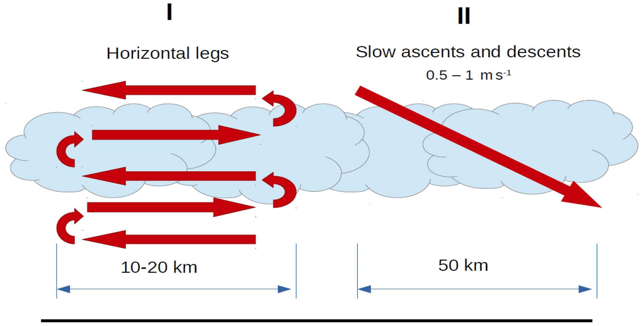
Figure 1 Flight pattern in clouds showing staggered horizontal legs and slanted profiles. Turns between legs were not included in the data analyses.

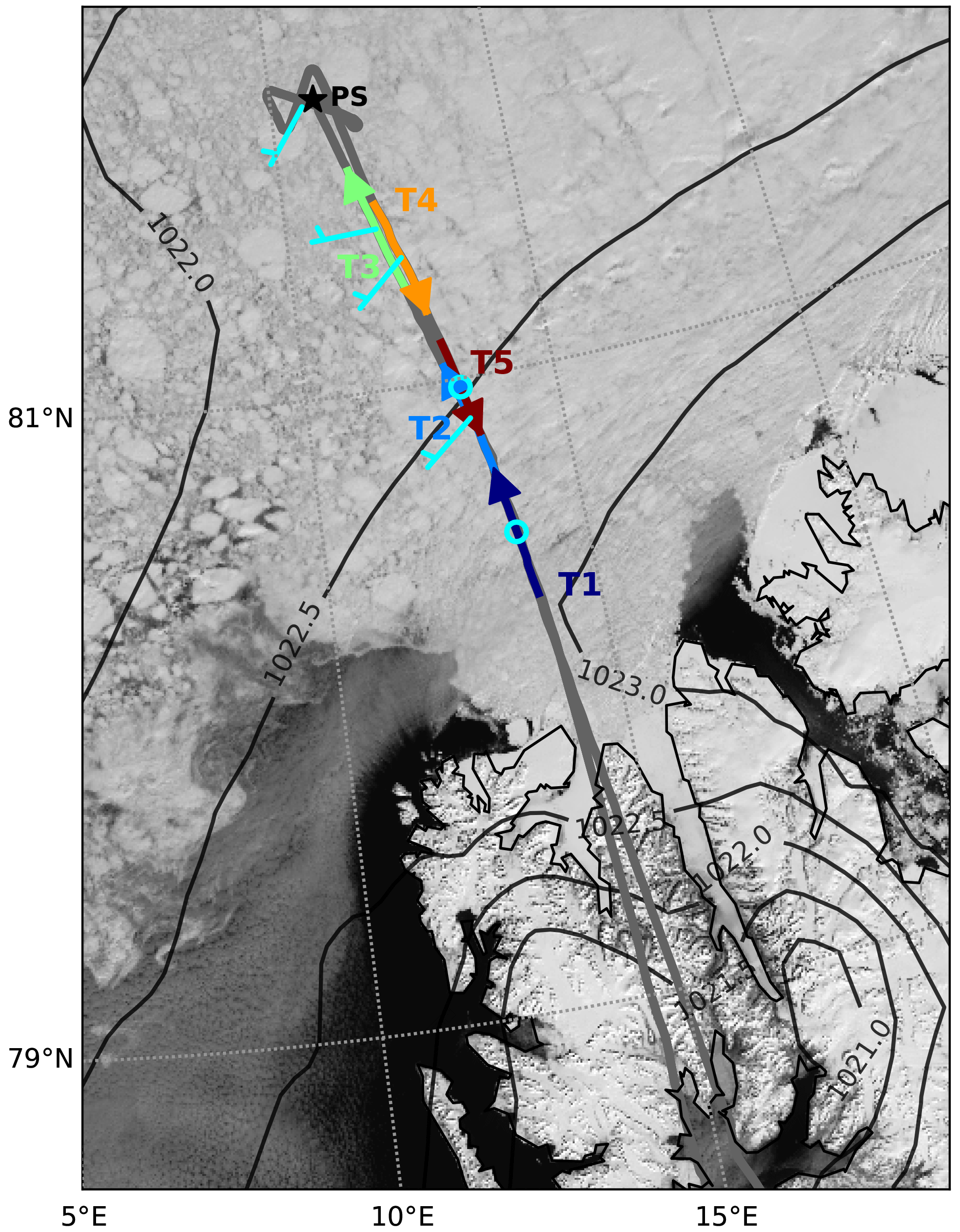
Figure 2 Polar 6 track on 5 June 2017 overlaid over the MODIS satellite image. T1–T5 represent descents and ascents of the aircraft, and PS is the position of RV Polarstern. Wind barbs indicate the ABL averaged wind. The barbs are plotted for wind stronger than 2.5 knots, while weaker wind is indicated by an open circle. Isobars represent the mean sea level pressure field based on the ERA5 reanalysis (Hersbach et al., 2020).

The drawback of these horizontal patterns is that the vertical resolution of a related flux profile is limited. For this reason we also used slanted profiles (see Fig. 1) with low ascending and descending rates of about 0.5 to 1.5 m s⁻¹. This method has been used earlier by Mahrt (1985), Lenschow et al. (1988), Tjernström (1993) and Aliabadi et al. (2016). Turbulence statistics were calculated using a moving window of about 100 s width corresponding with a layer of 100 m thickness and with a flight distance of about 5–10 km. Within each moving window a polynomial trend was removed. One can interpret the obtained profiles in a way that every point represents an approximation of the true values averaged over the corresponding height interval. Thus, this method provides continuous vertical profiles but suffers from two drawbacks: (1) relatively short time spent at a certain height resulting in a higher statistical uncertainty and (2) smoothing of the vertical profiles. It should be stressed that the obtained statistics from slanted profiles do not strictly approximate the values from horizontal legs, except the cases when turbulence statistics change with height very slowly. It is important that the flight segments crossing the inversion at the ABL top are excluded from the analysis of slanted profiles so that the considered profiles start below the ABL top, and steep jumps of quantities like temperature and wind components in the capping inversion are not misinterpreted as turbulence effects.

As in Tetzlaff et al. (2015), who considered measurements over sea ice with sometimes also low values of heat fluxes, we show in Appendix A that the accuracy of the used turbulence probe was sufficiently high in the horizontal legs to measure heat fluxes in the range of at least 5 W m⁻². Also in Appendix A, specific uncertainties related to measurements in clouds are addressed. Comparison of the results of the two different aircraft and the plausibility of obtained profiles points to even higher accuracy (see Fig. 13 and its description).

3 Results

The main goal of our analysis is to discuss the variability of the cloud impact and to explain the differences between the observed cases. This will be done on the basis of mean variables but also on the basis of turbulent moments such as the vertical fluxes of sensible heat H and components of momentum fluxes M_u and M_v. Here, the wind vector was rotated so that the u component is pointing into the mean wind direction averaged over the boundary layer, and the v component points to the orthogonal direction. Furthermore, we consider the turbulent kinetic energy (TKE); the variances of velocity components (also after rotation) ${\mathit{\sigma }}_u^{\mathrm{2}}$, ${\mathit{\sigma }}_v^{\mathrm{2}}$ and ${\mathit{\sigma }}_w^{\mathrm{2}}$ and of potential temperature ${\mathit{\sigma }}_{\mathit{\theta }}^{\mathrm{2}}$; the skewness of vertical velocity $S_w=\stackrel{\mathrm{‾}}{{w^{\prime }}^{\mathrm{3}}}/{\stackrel{\mathrm{‾}}{{w^{\prime }}^{\mathrm{2}}}}^{\mathrm{3}/\mathrm{2}}$; the vertical turbulent transport of potential temperature flux $T_{\mathrm{SH}}=\stackrel{\mathrm{‾}}{{w^{\prime }}^{\mathrm{2}}{\mathit{\theta }}^{\prime }}$; and the vertical transport of potential temperature variance $T_{\mathrm{TV}}=\stackrel{\mathrm{‾}}{w^{\prime }{{\mathit{\theta }}^{\prime }}^{\mathrm{2}}}$.

The description of cases does not follow a chronological order but starts with two single-layer low cloud cases and ends with multi-layer cloud cases. A weak-wind single-layer case is described first in detail because it serves as a reference case where the cloud effect on the ABL structure was clearly dominant throughout the ABL.

3.1 A single-layer cloud case with weak wind (5 June 2017)

On 5 June, a single-layer stratocumulus deck was present over the sea ice to the north of Svalbard. On the MODIS image one can see the contours of sea ice floes (Fig. 2) through the cloud layer; however, the clouds found during the flight, 2 hours after the satellite overpass, appeared opaque (Fig. 3f). The region of observations was over sea ice only on the periphery of an atmospheric high-pressure ridge, with weak horizontal pressure gradients causing a weak southwesterly flow along the flight track in the lowest 500 m over the surface.

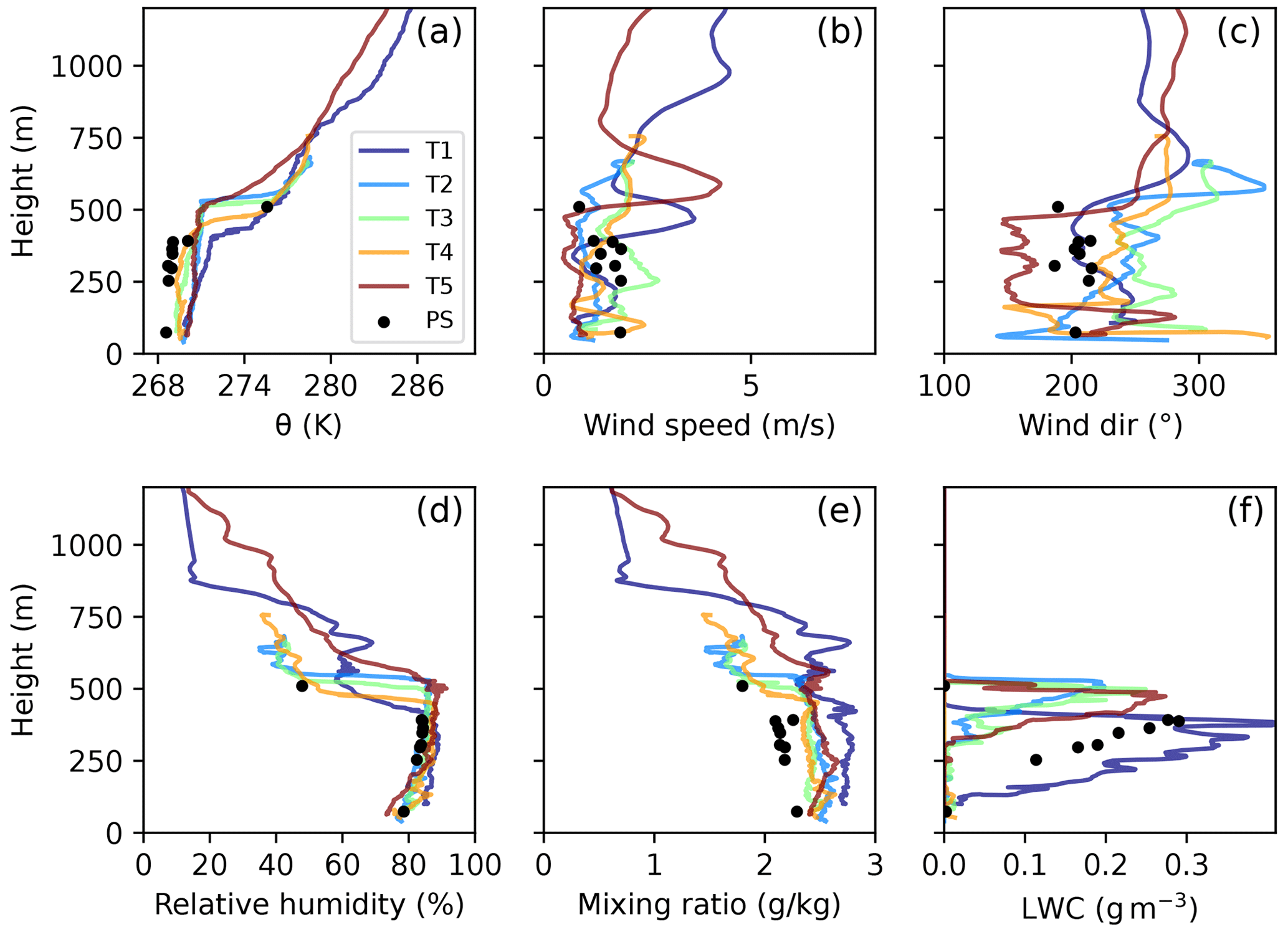
Figure 3 Vertical profiles of the mean potential temperature, wind speed and direction, absolute and specific humidity, and the liquid water content obtained during slant ascents and descents of Polar 6 on its way to PS and back on 5 June 2017. The locations of the ascents and descents are shown in Fig. 2.

On the way north to PS and back to south, Polar 6 was performing slow ascents and descents (saw-tooth profiling), as shown by colored segments in Fig. 2. Over PS, Polar 6 performed a double-triangle pattern with horizontal legs in different altitudes. Clearly, all profiles were obtained over sea ice, but patches of open water (lead-like structures) were also observed. In the following, the results of horizontal flight legs over PS and of slanted profiles along the track from T1 to the ship and back are discussed.

Table 1 The characteristics of the observed profiles on 5 June 2017.

The values of w_* and θ_* are calculated using Eqs. (C14)–(C16) with the observed heat flux profiles.

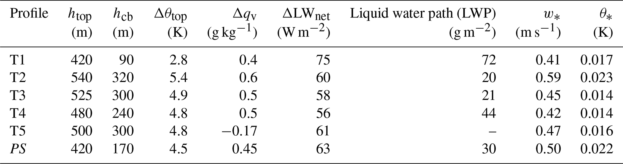
We first consider Fig. 3, showing vertical profiles of dynamic and thermodynamic parameters measured during profile patterns introduced in Fig. 1. The profiles document similarities at the different positions but also certain variability. The main characteristics of the shallow boundary layer are summarized in Table 1.

We find the following most important features. All profiles of potential temperature (Fig. 3a) indicate that the ABL was well mixed and capped by a sharp temperature inversion at the cloud top around 400 to 500 m height. The latter is visible from the LWC shown in Fig. 3f. The temperature inversions went along with strong jumps in relative humidity at the cloud top (Fig. 3d). Also the mixing ratio decreased above the cloud, although less pronounced and with some variability allowing small maxima (Fig. 3e) right above the cloud top and some of them still within the capping inversion. This phenomenon is best seen at T1 but also at T5 where another maximum occurs also 200 m above the cloud top. We point to this because such maxima and their possible origins have been described, e.g., by Egerer et al. (2021), who found a stronger maximum at the PS location on the same day using a tethered balloon. However, the aircraft measurements point to the spatial variability of the phenomenon.

The ABL wind was very weak with a horizontal speed of 1 to 2 m s⁻¹. In the southern profiles (profiles T1 and T5 in Fig. 3b), a low-level jet was present above the mixed layer. Vertical profiles of wind direction (Fig. 3c) show that wind appeared rather uniform in the cloud layer (visible from Fig. 3f), while a step change in direction below the cloud base is clearly visible in several profiles, especially at T4 and T5. This might hint to a decoupling between the well-mixed cloud layer and the surface-based boundary layer in some profiles but might also represent random variability. At the same time, the potential temperature and specific humidity profiles show no signs of decoupling.

The ABL variability along the considered track was most obvious in the LWC profiles (Fig. 3f), showing LWC-maxima between 0.2 and 0.35 g m⁻³. Cloud bases were between 100 and 300 m and thus were more variable than cloud tops (see above). As it is typical for a well-mixed stratocumulus layer, the LWC was increasing almost linearly with height with the same slope in all profiles. This was confirmed also by the results of the averaged horizontal flight legs.

In the case investigated here, a strong cloud-top cooling was present in all profiles (see radiation profiles in Appendix B). The jump of the net terrestrial energy flux LW_net across the cloud-top layer was in the range of 50 to 70 W m⁻² (Fig. B1). We assume here that LW_net is positive when the net flux is directed upward (as in, e.g., Nicholls and Leighton, 1986, their Fig. 7). The impact of the radiative cloud-top cooling is obvious in the profiles of turbulence moments discussed in the following.

To allow a comparison of the fluxes measured at positions T1 to T5 and at PS we introduce the scaling

$$z^{\prime }={\displaystyle \frac{z-c_{\mathrm{b}}}{h-c_{\mathrm{b}}}}\mathrm{if}z\ge c_{\mathrm{b}}$$

and

$$\begin{array}{}\text{(1)}& z^{\prime }={\displaystyle \frac{z-c_{\mathrm{b}}}{c_{\mathrm{b}}}}\mathrm{if}z<c_{\mathrm{b}}\end{array}$$

of the vertical axis, where z is height, h is cloud top and c_b is cloud base.

Figure 4 Vertical profiles of turbulence statistics obtained from horizontal legs over PS (black crosses) and slanted profiles on 5 June 2017. Red lines represent mean values based on four slanted profiles, while red shading indicates ± 1 standard deviation. The cloud layer as observed over PS is shown with grey shading.

In Fig. 4 we show the results of the slanted profiles and of the horizontal sections. For their comparison one should keep in mind their horizontal distance from each other. This may explain some of the differences between both types of results. However, the main characteristics are similar. For example, the values of turbulent heat flux H were clearly upward in the cloud and reached maxima of about 10 W m⁻². This was slightly larger than in the layer below the cloud, where at PS the surface-generated convective conditions led to clearly upward fluxes. In the subcloud layer H was near zero at the positions of the slanted profiles (Fig. 4a). Thus, the profiles of H deviated from a shape typical for quasi-stationary convective ABLs developing over a heated surface, where H decreases linearly with height. Obviously, positive heat flux was generated by the cold downdrafts (due to cloud-top cooling) and warm updrafts. At the cloud top, one would expect a substantial negative heat flux due to entrainment considering the presence of a temperature jump across the inversion. But only at PS was the value of H negative near the ABL top (about −3 to −4 W m⁻²) and thus downward. A possible reason is that capturing the downward fluxes is difficult especially for the slanted profile flights due to the very shallow inversion layer, but besides that the maximum in the spread of H near cloud base possibly also indicates that the heat flux was carried by eddies of varying size, some of which did and some of which did not penetrate below the cloud base.

Values of both components of the momentum flux were similar, which is due to the very low wind speed so that mainly convective mixing rather than wind shear was responsible. Nevertheless, directional shear was present at the cloud top and below the cloud base and might also have influenced momentum flux profiles. It can be seen that both components were increasing with height in the cloud with the largest negative values at the cloud base. Below the cloud, both components decreased with height and they were near zero in the layer reached by the aircraft below the cloud (Fig. 4b). Negative and positive values were found close to the cloud top. The scatter in that region is most probably associated with the variability of mixing in the entrainment zone (intermittency) but also with the measurement uncertainty (see below and Sect. 4).

The positive heat flux within the cloud layer as a consequence of the radiative cooling at the cloud top was responsible for the TKE generation in the cloud as well as for the maximum in ${\mathit{\sigma }}_w^{\mathrm{2}}$ (Fig. 4d, f) in the upper portion of the mixed layer. The latter is typical for upside-down convection and differs from Lenschow et al. (1980), who find the maximum of ${\mathit{\sigma }}_w^{\mathrm{2}}$ in the lower portion of a strong convective, surface-forced ABL. TKE was slightly elevated in the cloud layer below $z^{\prime }=\mathrm{0.9}$ (Fig. 4f). Both σ_u and σ_v were nearly constant with height and of the same size (Fig. 4d, e), apart from the region below the ABL top. Such a turbulence structure is typical for convective turbulence in a stratocumulus-topped ABL also in lower latitudes (Nicholls, 1984, 1989). But TKE and σ_u have some large values in the results of horizontal sections close to the cloud top. These maxima could be related to the observed directional wind shear across the inversion, as discussed in Sect. 4.

Other evidence of the upside-down convection was the negative skewness S_w of vertical velocity throughout the cloud layer (Fig. 4g). Close to the cloud top, S_w was close to zero. Such a structure of S_w in the Arctic stratocumulus was reported earlier by Sedlar and Shupe (2014), as well as by Hogan et al. (2009) based on radar and lidar data. In the subcloud layer, a sharp transition of S_w to zero or small positive values is observed. This might represent a transition from the upside-down convection in the cloud layer to the turbulence generated by shear or slight heating from the surface.

It is also important to consider the turbulent transport of heat flux T_SH (Fig. 4h). In nonlocal turbulence closure schemes this term is seen as the origin of the nonlocal, sometimes also called “countergradient”, transport by large eddies (e.g., Zilitinkevich et al., 1999). We see here again a structure pointing to upside-down forcing, namely downward transport in the cloud layer.

Another third moment, namely the transport of temperature variance T_TV (Fig. 4i), is also associated with nonlocal transport by large eddies. In the considered case, T_TV had a similar vertical structure to T_SH, with negative values in the cloud layer. It should be noted that only two horizontal flight segments show substantial negative values of T_SH and T_TV in the cloud layer. However, vertical profiles of T_SH and T_TV based on slanted profiles provide clear evidence of negative T_SH and T_TV in the cloud.

Based on the considered vertical profiles of turbulence statistics, as well as on the profile of mean wind direction (Fig. 3c), we can conclude that the fully mixed layer associated with the cloud was perhaps weakly coupled to the surface-based mixed layer. As discussed above, this is most obvious in the vertical profile of S_w. The absolute values of other statistics such as H, σ_u, σ_v, TKE, T_SH and T_TV also show a slight yet clear decrease in the subcloud layer. It is important to note that based on horizontal legs alone it would be harder to observe this. This shows the advantage of considering slanted profiles together with level flights.

Figure 4c also shows an increased temperature variance close to the ABL top. This is typical for convective and cloud-topped ABLs and is related to the entrainment of air from the inversion layer with a strong temperature gradient (Nicholls, 1984, 1989). Young (1988) found that one of the reasons for the increasing variance of θ at the top of a strong convective ABL is the forcing by the vertical gradient of temperature rather than turbulent transport of the temperature variance through the capping inversion. This is confirmed here since at the cloud top T_TV is near zero. But the visually observed undulating cloud top, as well as possible gravity waves in the stably stratified inversion layer, might have also contributed to an increased temperature variance near the capping inversion.

3.2 A single-layer cloud case with strong wind (2 June 2017)

Another single-layer stratocumulus case observed during ACLOUD on 2 June represents a flow directed almost parallel to the MIZ but with a slight on-ice flow component. It differs from the 5 June case by a stronger wind and stronger horizontal gradients of the ABL height and temperature. Another difference is that the flight was performed not only over sea ice as the flight on 5 June, but also the first part was over open water and thus, as discussed further, strong horizontal inhomogeneity in the cloud field was observed along the flight track from south to north. On that day, Polar 6 performed saw-tooth profiling over open water and sea ice on the way north and a double-triangle pattern in the cloud-topped boundary layer over sea ice at the northern end of the track (Fig. 5).

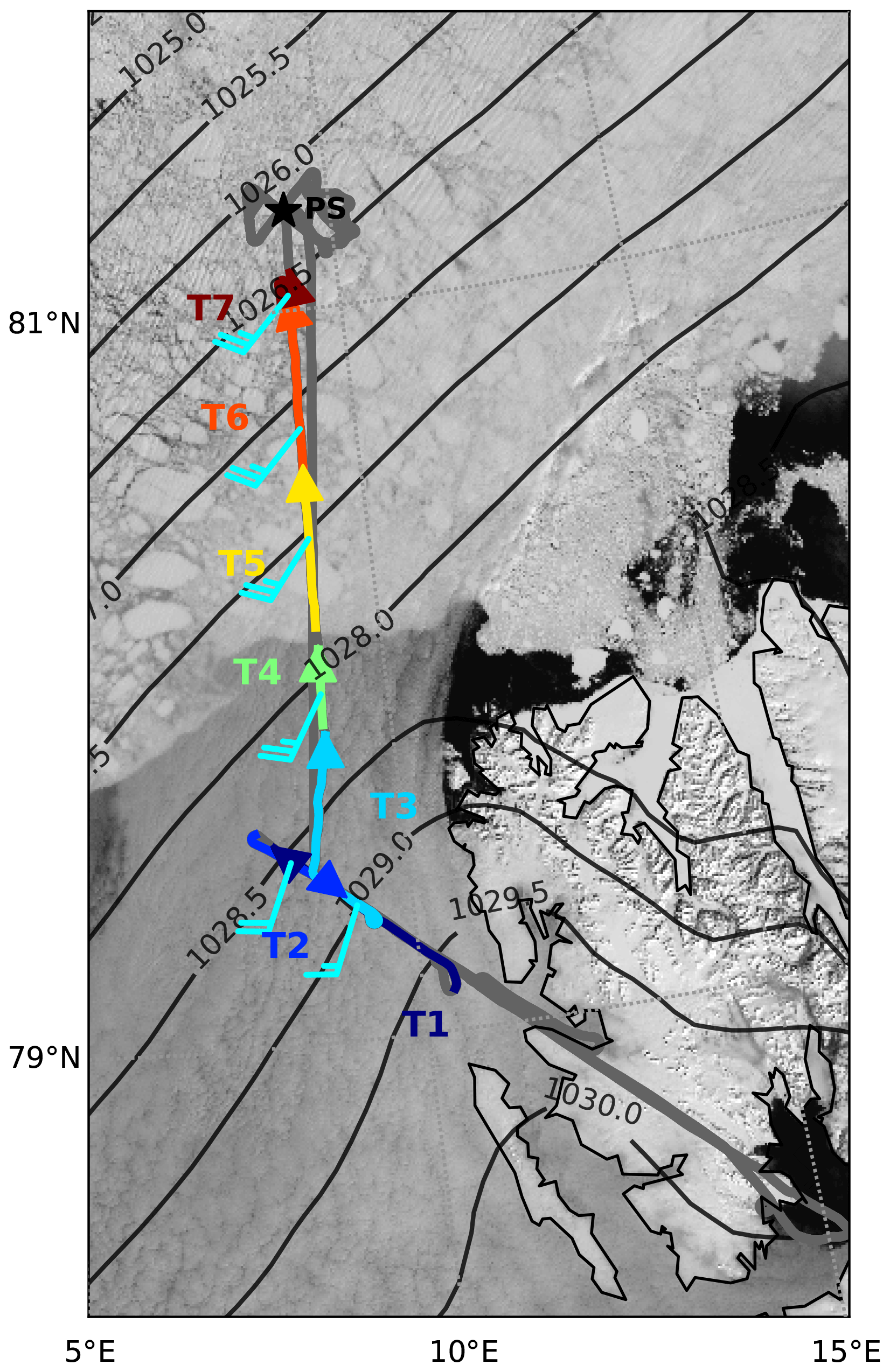
Figure 5 Polar 6 flight track on 2 June 2017 overlaid on the MODIS satellite image. T1–T7 represent descents and ascents of the aircraft. The wind barbs are showing the wind speed and direction averaged over the profile segments within the ABL. Isobars represent the mean sea level pressure field based on the ERA5 reanalysis.

Figure 6 shows vertical profiles of mean variables as observed during the saw-tooth ascents and descents. Clearly, a thick mixed layer was present over the open water up to about 750–800 m height (profiles T1, T2 and T3). The ABL height gradually decreased along the south–north flight track and reached about 350–400 m in the northernmost profiles T6 and T7. The cloud layer thickness also decreased from 500 m in the southern profiles to 250–300 m in the northern profiles (Fig. 6f). A strong capping inversion was observed over both open water and sea ice. The magnitude of the temperature jump at the cloud top reached 5 to 7 K (Fig. 6a). Drier air was lying over the ABL and the jump-like decrease of the mixing ratio was about 2 g kg⁻¹ across the cloud top (Fig. 6e).

Figure 6 Vertical profiles of the mean potential temperature, wind speed and direction, absolute and specific humidity, and the liquid water content obtained during slant ascents and descents of Polar 6 on its way to and from Polarstern on 2 June 2017. The locations of the ascents and descents are shown in Fig. 5.

All wind speed profiles show a decrease of wind speed towards the mixed-layer top, either starting from the lowest measuring level (profiles over water) or from a maximum in a low-level jet as in the profiles over sea ice (Fig. 6b). There, wind speed was highest (profiles T5 and T6) and reached about 14 m s⁻¹. Such a low-level jet could have been produced by the sloping inversion. As shown by Chechin and Lüpkes (2017), the increase of the ABL height towards the south in the presence of a capping inversion would result in an increase of the easterly wind component in the ABL.

The main reason for such a south–north variability of the ABL height and temperature might have been that the ABL wind was not directed along the flight track but from the southwest (220^∘). Thus, air parcels that arrived at positions T6 and T7 were influenced by sea ice in the MIZ, while T1–T3 rather represent open ocean conditions.

For the presentation of turbulence statistics, in the following we use $z/h$ as the vertical coordinate and not the more complicated z^′ as for 5 June. This is done, although again several profiles are considered (slanted profiles T5 and T6 and horizontal legs over Polarstern), at various positions and with different values of the ABL height h. However, the ratio $c_{\mathrm{b}}/h$, where c_b is the cloud-base height, is about the same for these profiles. Thus, using z^′ would not result in any difference as compared to using simply $z/h$.

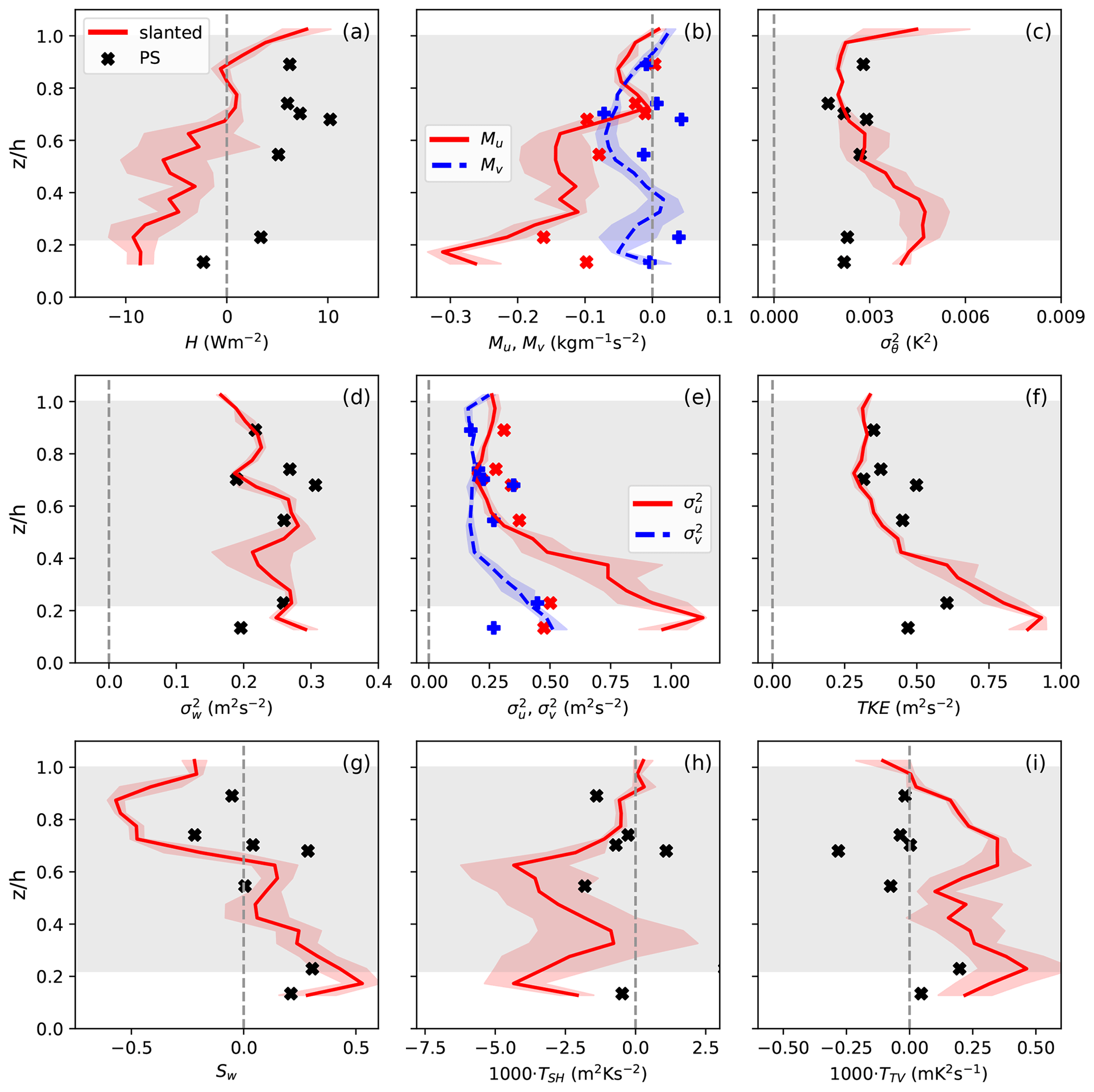
Figure 7 Vertical profiles of turbulence statistics obtained from horizontal legs over PS (black crosses) and slanted profiles T5 and T6 on 2 June 2017. Red lines represent mean values based on slanted profiles, while red shading indicates ±1 standard deviation. The cloud layer as observed over PS is shown with grey shading.

Similar to the 5 June case, a strong cloud-top terrestrial radiative cooling was present on 2 June both over open water and sea ice. The cooling rates were similar, with about −9 K h⁻¹ maximum cooling for all profiles independent of being over sea ice or open water (Fig. B1). The cooling explains some of the observed characteristics of the turbulent structure. Over sea ice, these characteristics differ strongly from those of the 5 June case. This becomes clear from a comparison of the results from slanted profiles shown in Fig. 4 with those in Fig. 7 (Profiles T5 and T6). The main difference is the occurrence of a pronounced TKE maximum in the lower portion of the ABL on 2 June, which does not exist on 5 June. It is clearly related to the maxima of ${\mathit{\sigma }}_u^{\mathrm{2}}$ and ${\mathit{\sigma }}_v^{\mathrm{2}}$ and not to the maximum of ${\mathit{\sigma }}_w^{\mathrm{2}}$. Near the surface, the absolute values of ${\mathit{\sigma }}_u^{\mathrm{2}}$ and ${\mathit{\sigma }}_v^{\mathrm{2}}$ reach 1.0 and 0.5 m² s⁻² (during slanted profiles), respectively, which is 2 to 3 times larger than the largest value of σ_w. On 5 June, ${\mathit{\sigma }}_u^{\mathrm{2}}$ and ${\mathit{\sigma }}_v^{\mathrm{2}}$ were much smaller, and ${\mathit{\sigma }}_w^{\mathrm{2}}$ had a pronounced maximum in the upper portion of the ABL and thus in the cloud. Although the vertical resolution obtained by the horizontal legs is not high enough on 2 June to resolve the lower maximum, these measurements do not contradict the slanted profiles (Fig. 7). In the cloud layer, some values of σ_w are somewhat elevated relative to the value obtained by the lowest horizontal leg on 2 June. This hints to two sources of turbulence: one in the cloud layer and the second one close to the ground.

The downward increase of TKE towards maxima in the lower part of the ABL, which is most pronounced at positions T5 and T6, hints to the dominant role of the TKE production by wind shear. One can conclude furthermore that the overall buoyancy production of TKE was relatively small because only small positive values of sensible heat flux occurred in the cloud layer. In the lower part of the ABL we detected negative heat flux. The latter was due to the warm air advection over colder sea ice. Thus, the ABL was being cooled both at its top and bottom. The cooling at the ABL top produced negative vertical velocity skewness S_w close to the top. In the middle of the ABL, we observed a pronounced shift to positive values of S_w, indicating surface generated turbulence. Another evidence of the influence of the surface is positive T_TV in slanted profiles, which corresponds to the upward transfer of temperature variance.

We conclude that the surface was shaping the turbulence structure but slight cloud-generated turbulence was still present, although it did not govern the entire ABL turbulent structure.

3.3 Multi-layer cloud cases

3.3.1 A two-layer cloud case with a slightly unstable boundary layer (14 June 2017)

We consider results from 14 June obtained north of Svalbard, where the estimated sea ice fraction was about 90 %–95 % based on visual observations (Fig. 8). The air advected from the north was only slightly colder than the average surface temperature of the mixture of ice and water in leads and small polynyas. But this temperature difference was high enough for the development of a slightly unstable ABL in the lowermost 400 m. In contrast to the profiles shown in the previous sections, a mid-level cloud layer existed with the base at about 1900 m and top at 2400 m (see LWC in Fig. 9f). This cloud layer produced strong cloud-top radiative cooling, as can be concluded from LW_net, indicating a strong vertical divergence at the cloud top (Fig. B1e, f). There, the maximal cloud-top cooling rate amounted to about −11 K h⁻¹. In contrast, the lower cloud layer could not produce a pronounced cloud-top cooling because the loss of terrestrial radiation was compensated by the emission of the cloud base of the overlying cloud layer. This is obvious in the low vertical divergence of LW_net, which was much less pronounced at the top of the lower cloud layer at about 400 m and resulted in about a −1 K h⁻¹ cooling rate.

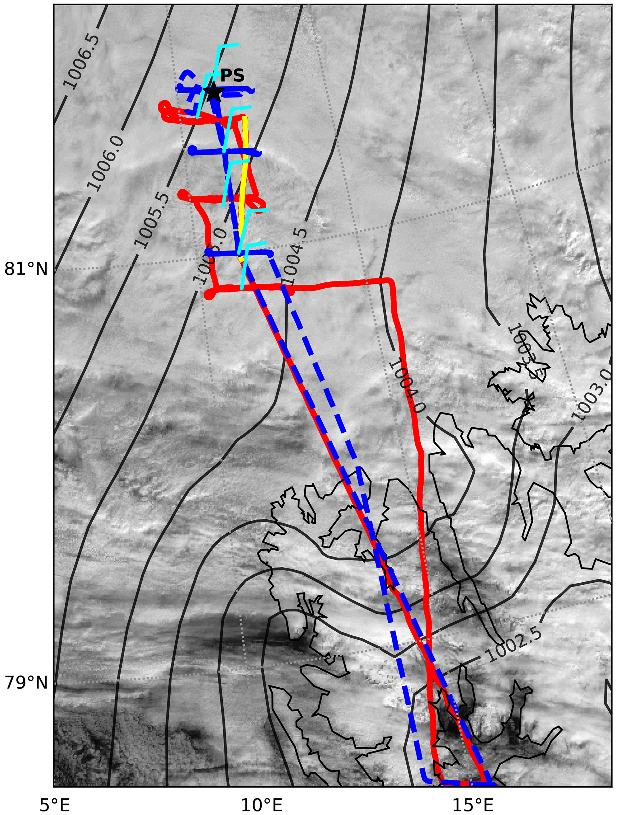
Figure 8 Tracks of Polar 5 (blue) and Polar 6 (red) on 14 June 2017 overlaid over MODIS satellite images. The wind barbs are showing the wind speed and direction averaged over the profile segments within the ABL. Only the northernmost cross-wind leg of Polar 6 and the two northernmost cross-wind legs of Polar 5 are analyzed. The yellow line marks the descend of Polar 6 used for the analysis.

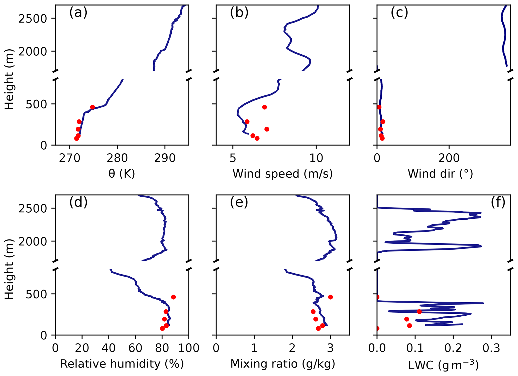
Figure 9 Results for 14 June 2017 obtained from a descent of Polar 6 in between the locations of the northernmost horizontal legs and the middle ones shown in Fig. 8.

Concerning the results of the horizontal flight sections, we concentrate here only on the three northernmost cross-wind staggered legs (Fig. 10). The reason is that in this region the surface and cloud conditions showed less variability between and along the different horizontal sections. Also, there were icing problems along the southern legs.

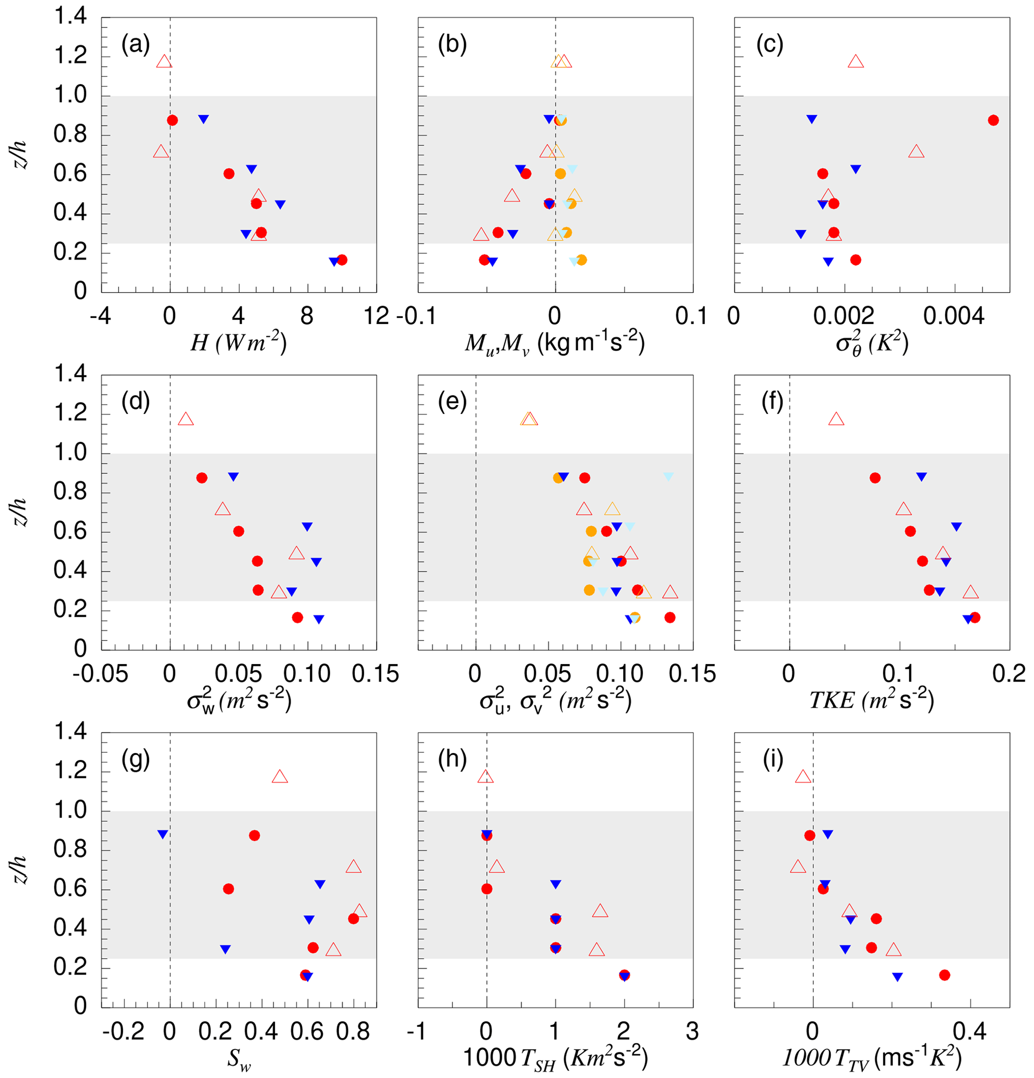
Figure 10 Turbulence statistics based on horizontal flight legs of 14 June 2017 obtained from Polar 5 (closed symbols) and Polar 6 (open symbols). Results of Polar 5 refer to the two northernmost dashed blue legs shown in Fig. 8. The Polar 6 result refers to its northernmost flight leg (red in Fig. 8). Altitude is normalized by the cloud-top height, h=400 m. The bright symbols (light blue and orange) refer to M_v and ${\mathit{\sigma }}_v^{\mathrm{2}}$, while the dark (red and blue) symbols in the corresponding panels refer to M_u and ${\mathit{\sigma }}_u^{\mathrm{2}}$.

Apparently, a well-mixed layer had developed below the cloud top. In the ABL, heat fluxes were directed upward and show a more or less linear decrease with height from values of about 10 W m⁻² at z=0.2h to 0 W m⁻² at the cloud top (z=h). This led to negative values of the bulk Richardson numbers Ri_b, where gradients of temperatures and wind entering Ri_b refer to the two lowermost legs. Values are ${\mathit{Ri}}_{\mathrm{b}}=-\mathrm{0.07}$, ${\mathit{Ri}}_{\mathrm{b}}=-\mathrm{0.05}$ and ${\mathit{Ri}}_{\mathrm{b}}=-\mathrm{0.20}$ from south to north (or $z/L=-\mathrm{0.34}$, −0.96 and −0.81, respectively, where z is the altitude of the lowest horizontal flight leg and L is the Obukhov length). Based on these values the regime in the observed case can be classified as convection with shear (e.g., Fedorovich and Conzemius, 2008).

Since the external conditions (temperature, wind, ABL top, cloud thickness) did not change substantially between the locations of the flight legs, it is expected that the turbulent quantities varied also very little. And indeed, despite the small signals, the accuracy of both aircraft data is obviously high enough to show very similar results at the different locations (Fig. 10).

It is interesting to compare this case with the cases observed on 2 and 5 June (see Figs. 4 and 7). While 5 June was purely cloud driven, 2 June was both cloud driven in the upper part of the ABL and surface driven in the lowest part. Both had a similar heat flux O(10)​​​​​​​ W m⁻² at the cloud top, caused by cloud-top cooling, which was obviously absent on 14 June. Thus on both days, 2 and 5 June, the heat flux profile with the maximum near the cloud top was reversed relative to the profile on 14 June with a maximum near the surface. Further differences are the following: on 14 June, the absolute values of ${\mathit{\sigma }}_w^{\mathrm{2}}$ and of TKE were only half as large as on 5 June despite stronger wind and positive surface heat flux on 14 June. ${\mathit{\sigma }}_w^{\mathrm{2}}$ and TKE were larger on 2 June than on both other days, obviously due to the much larger wind speed. Another difference to 2 and 5 June is that on 14 June the vertical transport of heat flux T_SH, of temperature variance T_TV and also S_w remained positive in the entire ABL (except near the capping inversion). This indicates once more that the processes were not cloud-top driven but surface driven. The reason for this different behavior is clearly the existence of the mid-level clouds, which led to a reduction of the cloud-top cooling and thus suppressed mixing at the cloud top.

3.3.2 A three-layer cloud case with a stable boundary layer (20 June 2017)

On 20 June, again a multi-layer cloud system was observed in westerly wind conditions and over a region with an ice fraction of about 95 % (Fig. 11). Figure 12 shows vertical profiles obtained during a descent of Polar 5 in the northern part of the observational area. No Nevzorov probe was installed on Polar 5, but visual observations and the vertical profile of relative humidity (Fig. 12b) allowed us to detect even three cloud layers with cloud tops at about 350, 2100 and 3000 m. The strongest cooling occurred at the uppermost cloud top, where the maximal cooling rate reached −10 K h⁻¹. Below that cloud top, the strongest turbulence and positive turbulent heat flux were also observed during the slanted descent (not shown here).

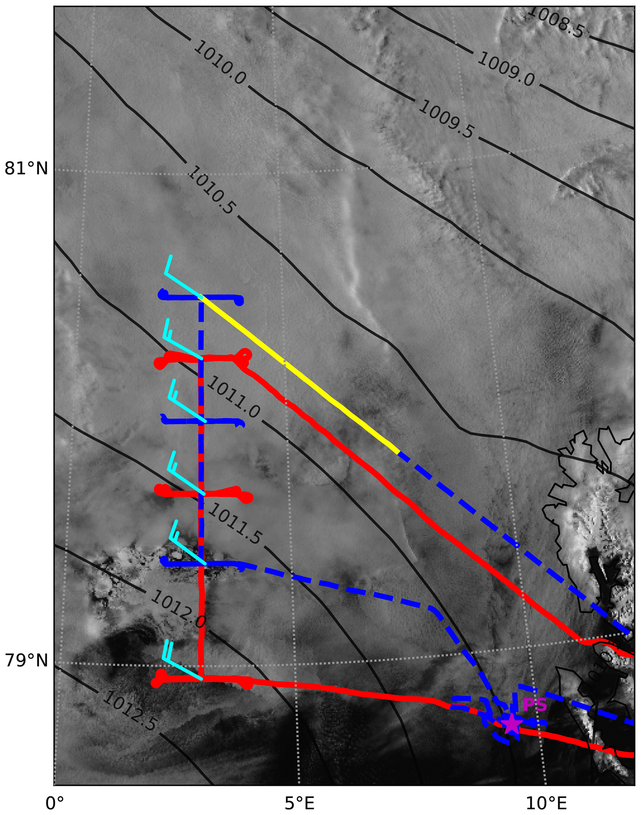
Figure 11 Tracks of Polar 5 (blue) and Polar 6 (red) on 20 June 2017 overlaid over the corresponding MODIS image. The yellow line refers to the Polar 5 descent shown in Fig. 12.

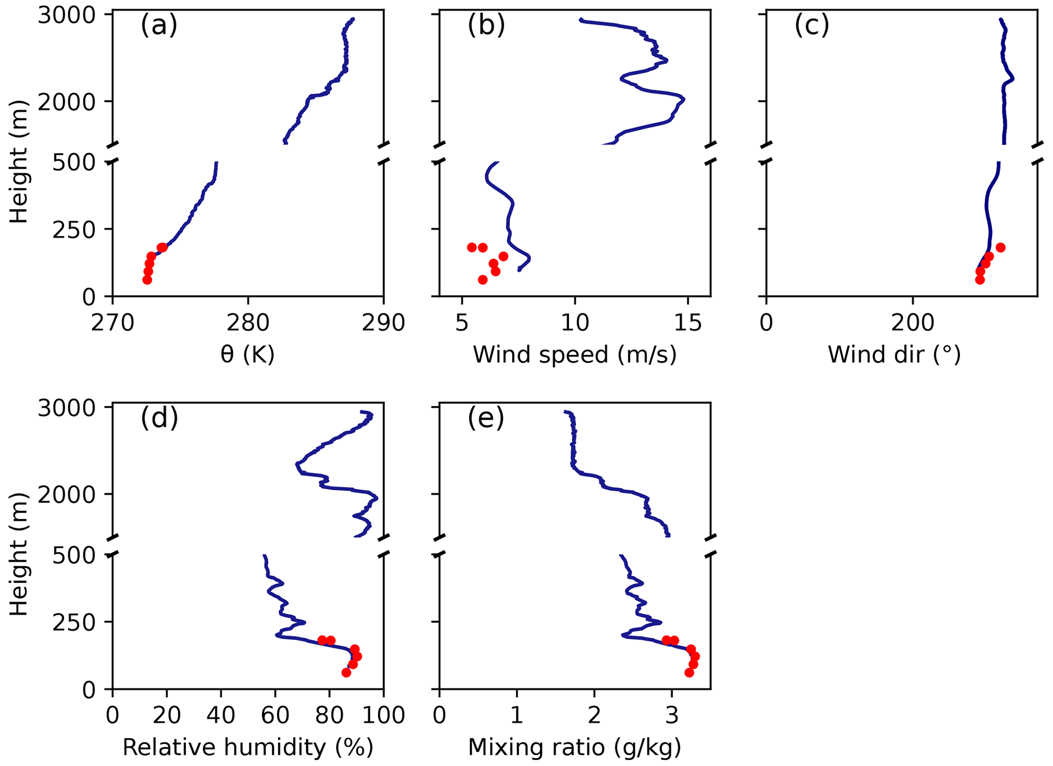
Figure 12 Results for 20 June 2017 obtained from a descent of Polar 5 at the location of the northernmost horizontal legs (see Fig. 11).

Figure 13 shows results for the lowest cloud layer and indicates a fundamental difference between the ABLs observed on this day and on 14 June. On 20 June, the westerly winds led to a near-surface stable stratification. This caused downward but very small absolute values of fluxes of sensible heat. The uncertainty of these values is in the order of the statistical error, nevertheless, the good qualitative agreement of all turbulent quantities obtained from both aircraft shows that the results are reliable enough to see the differences between the ABL structures of 5, 14 and 20 June. Turbulence decreased to almost zero at about z=h. This is roughly where the capping inversion started. Although no Nevzorov data were available for this flight, visual observations suggested that the cloud layer reached far into this capping inversion. This phenomenon was much more pronounced than on 14 March, when surface- and cloud-forced convection probably led to a well-mixed ABL.

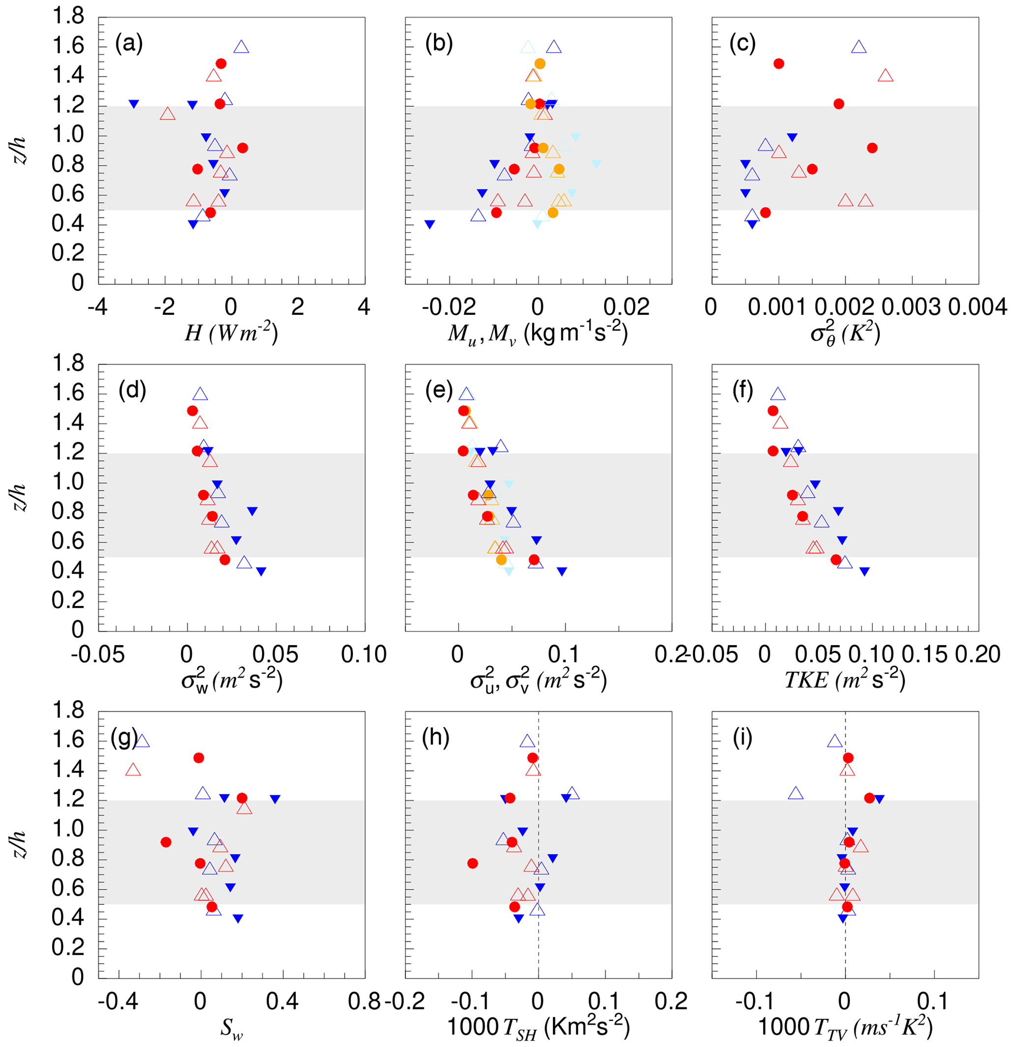
Figure 13 Turbulence statistics for the lowermost cloud layer based on the horizontal flight legs of 20 June 2017 obtained from Polar 5 (blue symbols) and Polar 6 (red symbols). The results refer to the two blue and red northernmost flight legs of the aircraft (see Fig. 11). Closed (open) symbols refer to the northern (southern) positions. Altitude is normalized by the cloud-top height for Polar 5 h=190 m (north) and h=225 m (south) and for Polar 6 h=250 m (both positions). The bright symbols (light blue and orange) refer to M_v and ${\mathit{\sigma }}_v^{\mathrm{2}}$, while the dark (red and blue) symbols in the corresponding panels refer to M_u and ${\mathit{\sigma }}_u^{\mathrm{2}}$.

To understand the differences between the results from both flight days with multi-layer clouds, it is important to note that the absolute wind speed did not differ much on these 2 d. Thus, differences between the days are most probably caused by the different density stratifications. The stability observed on 20 June caused strongly reduced values of ${\mathit{\sigma }}_w^{\mathrm{2}}$ (also of ${\mathit{\sigma }}_u^{\mathrm{2}}$ and ${\mathit{\sigma }}_v^{\mathrm{2}}$, not shown for 20 June) relative to the data on 14 June, and consequently the TKE was also much lower on 20 June. Variances and TKE decreased to zero at the cloud top, which is not really the case on 14 June. Nevertheless, despite the reduced values of TKE, a continuously turbulent ABL was observed on 20 June. This is in agreement with the observed values of stability parameters (Ri_b=0.16 and Ri_b=0.27 or $z/L=\mathrm{0.29}$ and $z/L=\mathrm{0.56}$, respectively, for the Polar 5 legs at the lowest heights), according to which the ABL state can be classified as slightly stable (e.g., Golder, 1972; Mohan and Siddiqui, 1998).

This comparison shows for both flight days with multiple cloud layers an impressive agreement between the measurements of both nosebooms installed on the two aircraft. This holds especially for the results of 20 June, when the signals from both nosebooms were very low but, nevertheless, very close to each other. Obviously, the situation was horizontally also very homogeneous; note that the maximum distance between legs was almost 150 km.

4 Discussion

It is important to compare the presented results with previous turbulence data sets obtained in liquid water clouds over Arctic sea ice. The largest data set was presented by Curry (1986) and Curry et al. (1988), who considered vertical profiles of mean variables and of turbulence statistics for six cases of summertime clouds in the Arctic.

First of all, we can confirm their conclusion that one of the differences of the Arctic stratocumulus clouds as compared to their marine counterparts in lower latitudes is the frequent occurrence of multiple cloud layers. Curry et al. (1988) concludes that, in such situations, strong turbulent mixing occurs in the uppermost cloud layer, which is decoupled from the surface. The lowermost cloud layer can occur as a kind of fog in a stably stratified boundary layer. Exactly such a scenario was observed also by us on 20 June, and thus it represents a further hint that such cases might be typical for the summertime Arctic.

However, the data set presented by Curry et al. (1988) does not contain a multi-layer case with an unstably stratified boundary layer, as we observed on 14 June. The comparison of the two multi-layer cases observed on 14 and 20 June reveals a strong difference in the magnitude of variances and of TKE. This highlights that surface fluxes may strongly affect the ABL turbulent structure even when boundary-layer clouds with low cloud base are present.

Curry (1986) compares the magnitude of the radiative flux divergence at the cloud top with the values of turbulent heat flux in the cloud and finds that only a small fraction of radiative cooling is compensated by turbulent heat transport. She further concludes that only “a small portion of cloud-top cooling results in the production of the mixed-layer convection”. Such a conclusion is based on the values of turbulent heat flux measured below the upper part of the cloud, where the strongest longwave cooling is observed (see Table 5 in Curry, 1986). Indeed, the reported values of the turbulent heat flux amount to about 3 W m⁻², which is lower than the 10–15 W m⁻² observed by us on 5 June. Our values are, however, still much lower than the jump of the net longwave radiative flux ΔLW across the cloud top. According to our observations, ΔLW is about 50–70 W m⁻² and thus similar to the values reported by Curry (1986). Therefore, the above-mentioned conclusions of Curry (1986) seem to be applicable also to our data, while the reasons behind it remain unclear.

To consider this matter in more detail, a simple mixed-layer model is utilized in the following. In particular, it is used to (i) understand why the observed turbulent heat flux is much smaller than ΔLW and (ii) estimate which portion of ΔLW is forcing the mixed-layer convection. Mixed-layer models of different complexity have been frequently used to describe stratocumulus-topped mixed layers (e.g., Lilly, 1968; Nicholls, 1984; Turton and Nicholls, 1987; Stevens, 2002), and the model used here is similar to the most simple ones formulated earlier (see details in Appendix C). The idea is that we use the observed profile of net terrestrial radiation as well as turbulent heat fluxes observed at the bottom of the mixed layer to diagnose the heat flux profile within the mixed layer. Furthermore, the model allows a calculation of the buoyancy forcing produced by longwave cooling and an estimation of the resulting vertical velocity variance. For the latter we use the Lenschow et al. (1980) parameterization as given by Eq. (C17).

First, the results of the mixed-layer model are compared with the observed profiles of H and ${\mathit{\sigma }}_w^{\mathrm{2}}$. The following scenario is considered for 5 June: the bottom of the mixed layer is assumed to be at 50 m height, where both sensible and latent heat fluxes are set to zero; the value of the liquid water potential temperature jump across the mixed layer is Δθ_l=6 K, while the jump of total specific humidity is set to $\mathrm{\Delta }{q}_{\mathrm{t}}=-\mathrm{0.5}$ g kg⁻¹. The cloud base is assumed to be at 170 m. Entrainment fluxes of θ_l and q_t are parameterized using Eqs. (C11) and (C13).

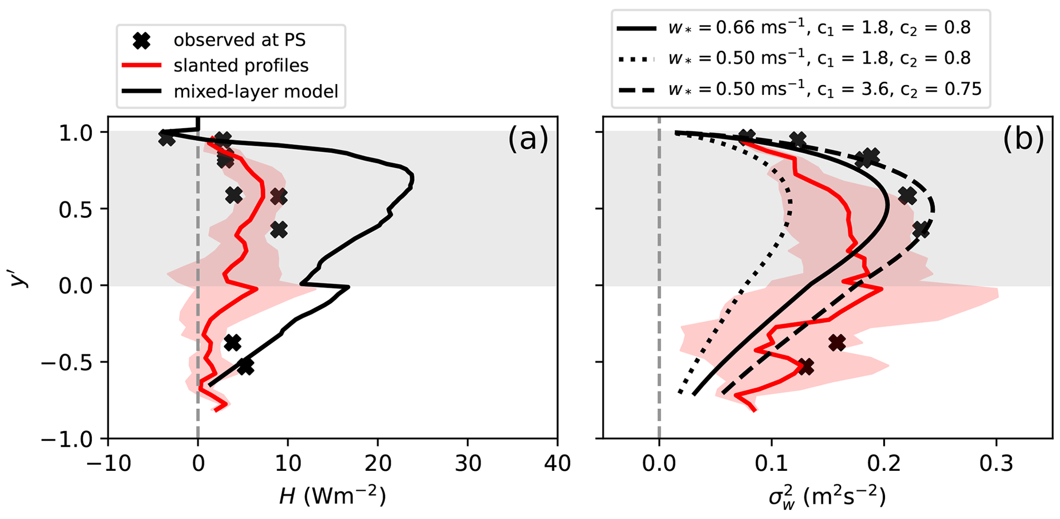
Figure 14 Observed and diagnosed turbulent heat flux profiles for 5 June (a) and vertical velocity variance (b) obtained using the Lenschow et al. (1980) parameterization (Eq. C17) with $w_{*}=\mathrm{0.5}$ m s⁻¹ and $w_{*}=\mathrm{0.66}$ m s⁻¹ and with modified constants c₁ and c₂.

Figure 14a shows the diagnosed sensible heat flux in comparison with the observed one. The mixed-layer model produces positive heat flux across the mixed-layer, with a maximum of about 20 W m⁻² located in the upper part of the cloud. This agrees qualitatively with observations; however, the model overestimates the flux by about a factor of 2.5. The diagnosed entrainment flux of sensible heat is about −4 W m⁻² which is very close to the observed one. Due to the overestimation of the sensible heat flux, the diagnosed value $w_{*}=\mathrm{0.66}$ m s⁻¹ exceeds the values 0.45–0.5 m s⁻¹ based on observations (see Table 1).

The low values of the observed heat flux in comparison to the diagnosed one might indirectly hint to a more negative entrainment heat flux than measured. In Finger and Wendling (1990), the entrainment heat flux amounted to about −20 W m⁻², which is about 5 times larger than in our case. Prescribing the value −20 W m⁻² at the top of the ABL in the mixed-layer model results in a decrease of the diagnosed heat flux in the cloud layer and in a good agreement with observations (not shown here). We should once more stress the difficulty to interpret observations near the capping inversion due to several factors such as undulating flight height, large vertical gradients of heat flux and undulations of the cloud top due to non-turbulent processes.

The parameterized profiles of ${\mathit{\sigma }}_w^{\mathrm{2}}$ using $w_{*}=\mathrm{0.5}$ m s⁻¹ (based on the observed heat flux profile) and $w_{*}=\mathrm{0.66}$ m s⁻¹ (based on the mixed-layer model heat flux profile) are shown in Fig. 14b. For both values, the shape of the profile is apparently well described by the Lenschow et al. (1980) parameterization (Eq. C17) including the location of the maximum. Despite the agreement of the shape, the smaller (and thus observed) value ($w_{*}=\mathrm{0.5}$ m s⁻¹) leads, however, to an underestimation of ${\mathit{\sigma }}_w^{\mathrm{2}}$ in the whole ABL when compared to the values from the horizontal legs. The larger value 0.66 m s⁻¹ shifts the parameterized ${\mathit{\sigma }}_w^{\mathrm{2}}$ profile closer to the observations. An even better fit to the observations can be obtained with $w_{*}=\mathrm{0.5}$ m s⁻¹ but only when the constants c₁=3.6 and c₂=0.75 are used in the Lenschow parameterization (dashed curve in Fig. 14b).

The question is why the observed ${\mathit{\sigma }}_w^{\mathrm{2}}$ is larger than ${\mathit{\sigma }}_w^{\mathrm{2}}$ calculated with w_* based on the observed heat flux profile. It is helpful to consider the ratio ${\mathit{\sigma }}_{w,max}/w_{*}$, where ${\mathit{\sigma }}_{w,max}$ is the maximum value of ${\mathit{\sigma }}_w^{\mathrm{2}}$. In particular, for $w_{*}=\mathrm{0.5}$ m s⁻¹ we obtain ${\mathit{\sigma }}_{w,max}/w_{*}\approx \mathrm{1}$, which is larger than the values obtained earlier. Previous studies report ${\mathit{\sigma }}_{w,max}/w_{*}\approx \mathrm{0.6}$–0.65 for stratocumulus in lower latitudes (Nicholls, 1984; Caughey et al., 1982; Deardorff, 1980) and in a convective boundary layer heated from below (Young, 1988). A possible explanation for this discrepancy is given by Smedman and Hoegstroem (1983), who showed that the ratio ${\mathit{\sigma }}_{w,max}/w_{*}$ is increased when wind shear contributes to the production of turbulence in addition to buoyancy. In the presence of shear, Finger and Wendling (1990) observed similar values of ${\mathit{\sigma }}_w^{\mathrm{2}}$ and heat flux as we did on 5 June, which would also result in ${\mathit{\sigma }}_{w,max}/w_{*}\approx \mathrm{1}$ in the cloud layer. In their case, the ABL wind speed was, however, much stronger and amounted to about 10 m s⁻¹. Although the wind speed was weak on 5 June, a directional wind shear was present at the cloud top and base (Fig. 3c), which might have contributed to TKE and ${\mathit{\sigma }}_w^{\mathrm{2}}$ production and would explain the large value of ${\mathit{\sigma }}_{w,max}/w_{*}$.

Thus, the mixed-layer diagnostics show several things. First, we can conclude that the heat fluxes observed by Curry (1986) in single-layer stratocumulus are much smaller than one would expect. Our observations are much closer to the mixed-layer model and are also in agreement with Finger and Wendling (1990) who observed turbulent heat fluxes of 10–15 W m⁻² in the cloud layer. Second, the mixed-layer model shows that the turbulent heat flux can indeed be several times smaller than ΔLW, and yet it is enough to redistribute the longwave cooling uniformly throughout the mixed layer, as explained in more detail as follows.

To understand why turbulent heat flux can be much smaller than ΔLW it is important to consider the following property of the mixed layer. Namely, the total flux of the conservative variable θ_l has to change linearly with height as expressed in Eq. (C3). There, the total flux is the sum of LW_net and $\stackrel{\mathrm{‾}}{w^{\prime }{\mathit{\theta }}_{\mathrm{l}}^{\prime }}$. Due to the fact that usually LW_net changes nonlinearly with height (Fig. B1), some amount of turbulent heat flux is needed to compensate for this nonlinearity. The needed amount of turbulent heat flux is proportional to how far from linear the LW_net profile is. Obviously, for a very thin layer (e.g., a layer between $z/h=\mathrm{0.8}$ and $z/h=\mathrm{1}$ in Fig. B1) LW_net alone is already close to linear so that there the cloud layer would cool almost uniformly with height even with a small amount of turbulent mixing. This is not the case for optically and geometrically thick mixed layers, where the strong longwave cooling in the upper part of the cloud layer generates a strongly nonlinear profile of LW_net. To obtain well-mixed profiles of the cloud liquid water potential temperature and cloud water mixing ratio, the loss of heat at the cloud top has to be redistributed then throughout the mixed layer by strong turbulent motions. In such thick clouds, the maximum of the turbulent heat flux would be closer to ΔLW. Apart from this, the presence of a negative entrainment flux also leads to a decrease of the turbulent heat flux maximum in the cloud because the entrainment is compensating for a part of the longwave cooling. Thus, we can conclude that in thin mixed layers, indeed, turbulent heat flux can be substantially smaller than the longwave cooling expressed by ΔLW. This explains why not the whole amount of ΔLW is used to force the mixed-layer convection.

In connection with the above discussion, one should also keep in mind the uncertainty of the observed turbulence statistics. The magnitude of the uncertainty for heat and momentum fluxes obtained from horizontal legs is discussed in Appendix A. Similar to earlier studies (e.g., Curry et al., 1988; Finger and Wendling, 1990; Inoue et al., 2005), the uncertainty is estimated empirically by comparing results from shorter segments of a long horizontal leg. Theoretical estimates of sampling errors due to an insufficient length of flight legs also exist (Lenschow and Stankov, 1986; Lenschow et al., 1994). Based on large Eddy simulation (LES), Petty (2021) showed that there is a good agreement between the empirical and theoretical estimates. However, neither theoretical estimates nor LES account for the horizontal non-turbulent inhomogeneities that exist in nature and complicate the analysis of the observations. It is even harder to obtain theoretical estimates for slanted profiles, as statistical properties of turbulence are functions of height within the ABL. Thus, we also rely on empirical estimates of the uncertainty for slanted profiles. So, we can consider the range of the slanted profiles (red hatched regions in Figs. 4 and 7) obtained at different positions as a measure of accuracy obtained from these profiles. This is not more than a rough estimate, and we expect that, especially near the inversion (above $z/h=\mathrm{0.8}$), the measurement errors are large for the slanted profiles but also for the horizontal legs. This hold also for previous aircraft campaigns (Lenschow and Stankov, 1986). In the future, flights should be performed repeating the same profiles and including horizontal flight legs at the same positions to determine the accuracy.

Finally, it should be noted that theoretically the uncertainty for third moments is higher than for the second ones. It can be reduced by considering longer averaging intervals, but the drawback of long horizontal legs is that horizontal inhomogeneity starts to affect the results. In case of slanted profiles, it is simply not possible to increase the leg length, as it will either cover a very large height interval or require a very slow ascent or descent, so that the horizontal distance flown during ascent/descent would become too large.

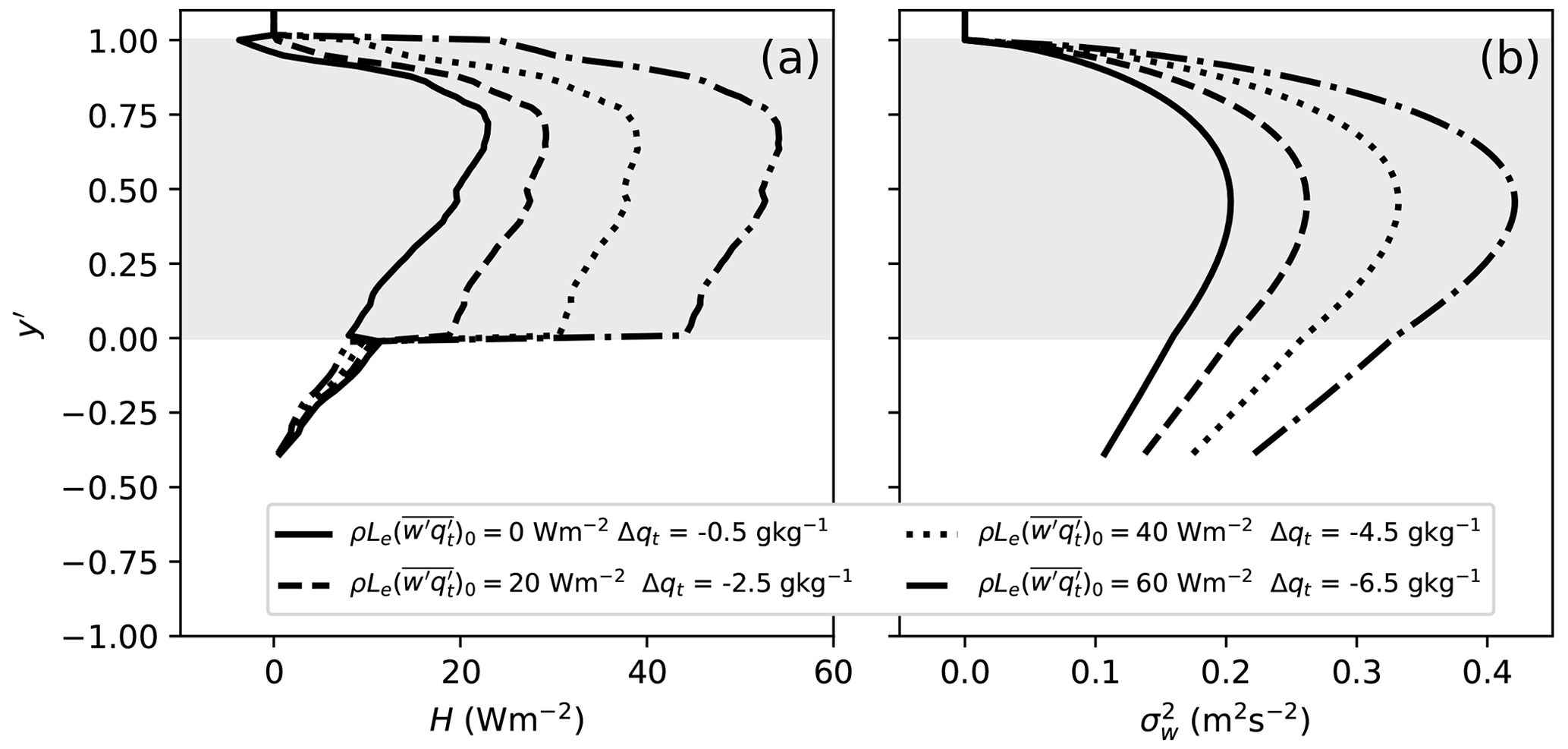
Figure 15 Sensitivity of the sensible heat flux profile (a) and vertical velocity variance (b) obtained from the mixed-layer model to the value of latent heat flux at the bottom of the mixed layer $\mathit{\rho }{L}_{\mathrm{e}}(\stackrel{\mathrm{‾}}{w^{\prime }{q}_{\mathrm{t}}^{\prime }}{)}_{\mathrm{0}}$ and to the value of the jump of total specific humidity at the top of the mixed layer Δq_t. Vertical velocity variance is obtained using the parameterization of Lenschow et al. (1980) (Eq. C17) with the original values of c₁ and c₂.

The mixed-layer model also highlights an important difference between the Arctic and subtropic stratocumulus. For subtropics, a substantial latent heat flux at the bottom of the mixed layer is typical, while at the top of the mixed layer dry air is entrained. In the mixed-layer model this leads to an increased buoyancy and heat flux in the cloud layer and consequently to a stronger turbulence. The reason for that is an increase of condensation and latent heat release in updrafts and evaporation and associated cooling in downdrafts. This is illustrated by the sensitivity experiments with the mixed-layer model (Fig. 15). The parameters of the experiments are the same as for the 5 June experiment, except that we prescribe a gradual increase of the latent heat flux at the bottom of the mixed layer as well as an increase of the total humidity jump at the top of the mixed layer. The typical values for subtropical stratocumulus are $\mathit{\rho }{L}_{\mathrm{e}}(\stackrel{\mathrm{‾}}{w^{\prime }{q}_{\mathrm{t}}^{\prime }}{)}_{\mathrm{0}}=\mathrm{115}$ W m⁻² and $\mathrm{\Delta }{q}_{\mathrm{t}}=-\mathrm{7.5}$ g kg⁻¹ (Duynkerke et al., 2004; Stevens et al., 2005). In contrast, in the Arctic the surface latent heat flux is small. During the ASCOS campaign, latent heat flux in the surface layer did not exceed 5 W m⁻² (Brooks et al., 2017). Furthermore, a humidity inversion often occurs at the top of the Arctic mixed layer, which leads to the entrainment of moist air. As a result, an increase of buoyancy is much smaller in the Arctic stratocumulus.

Table 2 Summary of the observed cases during ACLOUD in comparison with earlier turbulence observations in stratocumulus-topped ABL over the Arctic sea ice in summer.

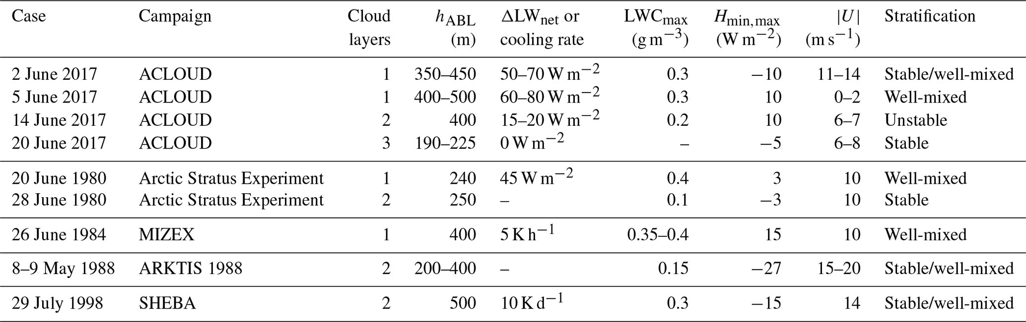
Cases are described in: Arctic Stratus Experiment (Curry et al., 1988), MIZEX (Finger and Wendling, 1990), ARKTIS 1988 (Brümmer et al., 1994), SHEBA (Inoue et al., 2005).

Table 2 summarizes the investigated cases together with observations from earlier studies. It shows that, to our knowledge, our study presents for the first time (i) a case with a strong cloud-top cooling and almost zero wind speed and (ii) two multi-layer cases with contrasting stability in the boundary layer. This broadens the parameter space with available observations, which is important for process understanding and model verification and testing.

5 Conclusions

We presented and analyzed airborne measurements of turbulence and radiation obtained during the campaign ACLOUD over the marginal sea ice zone to the north and northwest of Svalbard. By combining two types of flight patterns, namely staggered horizontal legs and slanted profiles, we obtained vertical profiles of turbulent quantities using the eddy covariance method. A combination of both flight patterns is shown to be clearly beneficial for the analysis of turbulence profiles.

The presented analysis attempts to distinguish the effect of clouds on turbulence statistics in comparison with the role of other mechanisms of turbulence generation. This was possible because one of the cases, namely 5 June 2017, was characterized by a near-zero wind speed in the ABL. Thus, the terrestrial radiative cooling at the cloud top was the only relevant mechanism of turbulence generation apart from a possible influence of directional wind shear, which was of secondary importance. To our knowledge, this is the first time that such a case of summertime stratocumulus over Arctic sea ice is presented. We showed that the cloud-top cooling is forcing upside-down convection, which shapes the ABL turbulent structure, especially in its upper part and during weak synoptic wind. In situations with only one cloud layer, the cloud impact is identified by local maxima of the vertical velocity variance and heat flux in the cloud layer, as well as by a negative vertical velocity skewness. In this respect, an Arctic stratocumulus-topped ABL is qualitatively similar to other cloud-topped ABLs in lower latitudes despite its shallowness and lower humidity.

We showed that strong cloud-top cooling causes the third moments $T_{\mathrm{SH}}=\stackrel{\mathrm{‾}}{{w^{\prime }}^{\mathrm{2}}{\mathit{\theta }}^{\prime }}$ and $T_{\mathrm{TV}}=\stackrel{\mathrm{‾}}{w^{\prime }{{\mathit{\theta }}^{\prime }}^{\mathrm{2}}}$ to be negative in the cloud layer, hinting at the possible importance of nonlocal transport associated with large eddies. However, this is only a hint, and quantifying the role of the third-order transport has to be a subject of a separate study. Here, we did not analyze the second-order moment budgets and thus cannot conclude on the relative role of various processes, as was done for a cloud-topped ABL in the LES-based study by Heinze et al. (2015).

Based on results of a mixed-layer model we showed that just a part of the net longwave cooling is forcing mixed-layer convection. In particular, the amount of sensible heat flux generated by the longwave cooling depends on how far from linear the profile of the net longwave flux is. Thus, the maximum of sensible heat flux in a boundary-layer cloud is expected to be small in a shallow mixed layer and large in a thick mixed layer. In particular, this explains why the observed heat flux maximum is much smaller than the jump of the net longwave flux across the upper part of the cloud. Thus, the amount of buoyancy forcing for the mixed-layer turbulence depends on the mixed-layer thickness.

In conditions with strong wind and a very shallow boundary layer, shear-generated turbulence played a more important role for the ABL turbulent structure than the cloud impact. This statement holds true even in the presence of strong cloud-top cooling. Namely, the strong-wind case that has been investigated was characterized by a pronounced maximum of the variance of all three velocity components and TKE located at low altitude in the subcloud layer.

When mid-level clouds were present, the cloud-top cooling in the lower cloud layer located in the ABL became substantially weaker. This resulted in a much weaker turbulence in the ABL even despite stronger wind. In such conditions, the ABL stability associated with surface–air temperature difference and wind speed apparently becomes an important factor influencing the ABL turbulence. This concerns both turbulence magnitude and the ABL turbulent structure.

To conclude, our results suggest that cloud-top cooling is one of the major sources of turbulence in the spring-summer Arctic ABL even despite its typical shallowness and relative dryness. We found that the amount of such cooling strongly depends on the presence of mid-level clouds, as concluded earlier also by other studies based on radar observations. The importance for the ABL structure depends, among other factors, mainly on wind speed, ABL height and stability.

Finally, based on mixed-layer model diagnostics, we showed that, despite qualitative similarities of the stratocumulus-topped boundary layers in the Arctic and lower latitudes, there are also substantial differences. In particular, low latent heat flux at the surface and small total specific humidity jump at the ABL top (or even a humidity inversion) result in a much lower buoyancy forcing as compared to subtropical stratocumulus. In addition, as already stressed above, in shallow mixed layers a smaller amount of turbulent heat transport is needed to redistribute the effect of cloud-top cooling across the mixed layer. This further decreases buoyancy heat flux in the mixed-layer. As a result, smaller magnitudes of turbulent heat flux maxima and TKE are expected in clouds over Arctic sea ice as compared to lower latitudes. The situation might be different, however, for clouds over open water, especially in the case of large air-sea temperature differences.

Thus, for an adequate representation of the ABL turbulence in coarse-resolution models a tight coupling between the radiative, microphysical and turbulence parameterizations is needed. The presented cases may serve as a reference for further studies focusing on the evaluation of such parameterizations.

We stress that the number of cases that we considered was limited and the results should motivate for future research. However, we have shown by a few cases that there is high complexity due to the many forcing parameters, but a detailed consideration helps to understand the mechanisms. Moreover, an understanding of these processes is relevant for the polar climate due to the strong impact on the energy fluxes. Future measurements would be helpful to further study the described phenomena.

Appendix A: Accuracy

Before ACLOUD the Polar 5 and 6 turbulence equipment was never used inside clouds and especially not in clouds above sea ice. Such conditions are challenging because, e.g., heat fluxes are mostly much smaller than in strong convective conditions over the open ocean in a surface-forced convective ABL during cold air advection (see airborne measurements described by Gryanik and Hartmann, 2002) or over leads described in earlier applications of the used turbulence probe by Tetzlaff et al. (2015). Thus, the accuracy of the measurements needs to be reconsidered. Moreover, as in earlier studies (Curry, 1986; Finger and Wendling, 1990) it is important to quantify empirically the uncertainty of the derived turbulence statistics. Apart from instrumentation characteristics, other factors influence the accuracy, as described in Sect. 2.2. The accuracy of the turbulence measurements in clouds will be considered in the following for the typical case of 5 June 2017.

On this day, eight horizontal flight legs were flown, one clearly below the cloud layer, five legs within the cloud and another leg two sections above the cloud. The cloud base and the cloud top have been observed at 200 and 400 m, respectively. Frequency-weighted power spectra for the three wind components, potential temperature and heat flux are shown in Fig. A1, as measured in the cloud. Spectra of u, v and w show the characteristic slope of $-\mathrm{2}/\mathrm{3}$ (corresponding to $-\mathrm{5}/\mathrm{3}$ without weighting) in the inertial subrange over more than 2 orders of magnitude. Similarly, the heat flux multiplied with the frequency shows the required $-\mathrm{4}/\mathrm{3}$ slope. Temperature variations at high frequencies (above 5 Hz) become very small and reach the detection limit. Thus the temperature variance spectra begin to exhibit some white noise beyond 5 Hz. However, this has no serious impact on the measured heat flux, which becomes obvious by considering the ogives O_w,θ representing the cumulative integration of the cospectrum Co_w,θ between the highest and lowest measured frequency (Friehe et al., 1991). Based on the ogives shown in Fig. A1 one can conclude that at least 95 % of the fluxes are caused by contributions below 1 Hz. Maxima for w and θ are between 0.1 and 0.2 Hz, depending on the aircraft height. This corresponds to wave lengths of about 1.5–3.5 km when we assume an average aircraft speed of 55 m s⁻¹. The ogive shows some deviation from an ideal S shape at the low frequency (large wave length) end of the spectrum. This might point to a too-short leg length; however, a prolongation would have led to other difficulties since, usually, homogeneity of turbulence is not guaranteed over distances larger than the 10–18 km during our measurements because of inhomogeneities in the cloud structures.

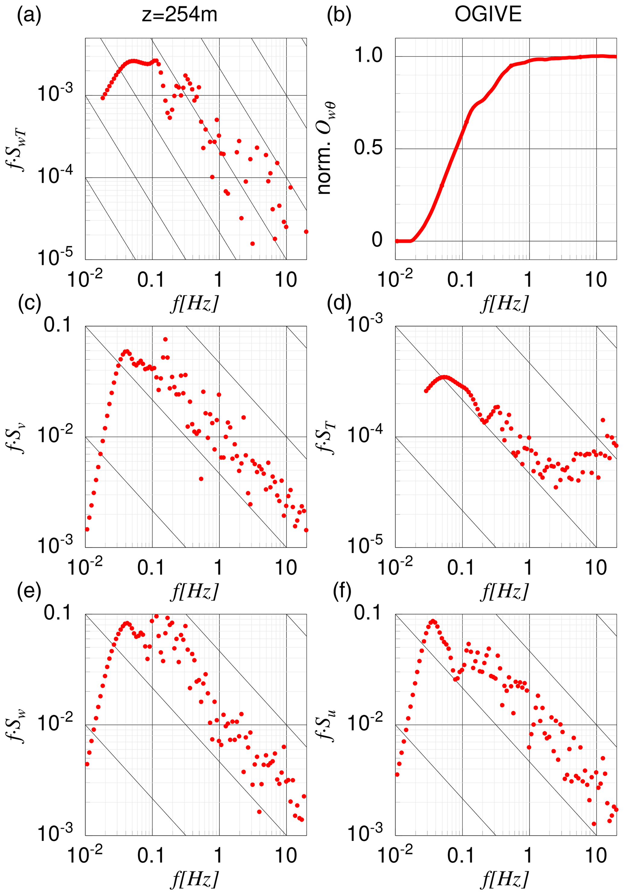
Figure A1 Frequency-weighted power spectra (S_u, S_v, S_w for wind components; S_t for temperature; and S_wT for temperature flux) and ogive O_w,θ as measured on 5 June 2017 in the cloud at 254 m height.

Also, in horizontal flight sections an aircraft cannot always fly exactly in one altitude. Especially in the uppermost part of the cloud with the capping inversion, the remaining fluctuation of aircraft height of about ±10 m is therefore correlated with changes of potential temperature caused by its vertical gradient. We corrected this impact on the temperature series based on the mean measured vertical temperature gradient along the flight leg. The impact of this correction is not large (in the range of the sampling error ϵ). ϵ was determined as in Friehe et al. (1991) depending on the leg length and flight altitude above the ground. Figure A2 also shows the momentum flux M with the corresponding ϵ.

Figure A2 (a) Fluxes of sensible heat and of absolute values of momentum as measured on 5 June 2017. Whiskers in both panels show the sampling error ϵ, determined following Friehe et al. (1991).

We also need to address, however, some uncertainty of air temperature observations in clouds caused by the evaporation of liquid from the sensing element (Lenschow and Pennell, 1974) and droplets during the adiabatic heating of air in the housing of the sensor (Lemone, 1980; Albrecht et al., 1979). We have to leave an experimental determination of this error for future research for the used Rosemount temperature sensor and can only speculate that the related error for turbulence is probably not too large in the cold Arctic conditions with relatively low absolute humidity. With respect to the accuracy of the temperature measurements, it is a good sign at least that the results of both aircraft agree well when flight legs have been flown close to each other (see Ehrlich et al., 2019) within a thin cloud at a distance of about 200 m. At such a distance one can expect that both temperature sensors have not been exposed to the same humidity conditions so that a possible error due to evaporation effects might have caused differences in the temperatures.

Also, in Sects. 3 and 4 we show that all vertical profiles can be physically well explained. This concerns both the profiles derived from horizontal flight legs and those from the slanted profile flights. Concerning the latter, we need to assume that the statistical error is probably larger as compared with the horizontal legs, so that especially those results need to be considered with some caution. Nevertheless, the results are at least reasonable. It is also important to see that profiles of different turbulence moments do not show contrasting results. This gives additional confidence in the data that is beyond the pure statistical evaluation and should also be kept in mind when the accuracy is considered.

Appendix B: Terrestrial radiation flux density and cooling rates

Figure B1 shows the net terrestrial radiative flux (left panels) as well as the radiative cooling rates in the atmospheric boundary layer for the considered cases. Note that on 14 and 20 June the strongest radiative cooling was observed in the upper cloud layers at heights of about 2500 and 3000 m (not shown here).

Figure B1 Vertical profiles of the net terrestrial radiative energy flux LW_net and of the cooling rate associated with the vertical divergence of LW_net. The altitude is normalized by the cloud-top height h so that individual profiles can be compared.

Appendix C: Diagnostic mixed-layer model

We choose the following variables that are approximately conservative during the moist-adiabatic processes in the mixed layer: the liquid water potential temperature θ_l and the total liquid water mixing ratio q_t. The latter two are defined as

$$\begin{array}{}\text{(C1)}& {\displaystyle }{\mathit{\theta }}_{\mathrm{l}}=\mathit{\theta }-\left({\displaystyle \frac{\mathit{\theta }}{T}}\right){\displaystyle \frac{L}{c_p}}{q}_{\mathrm{c}},\text{(C2)}& {\displaystyle }{q}_{\mathrm{t}}=q_{\mathrm{v}}+q_{\mathrm{c}},\end{array}$$

where L is the heat of vaporization, c_p is specific heat at constant pressure, q_c is the liquid water content and q_v is specific humidity. Below the cloud base, i.e., for z<h_cb we have simply θ_l=θ and q_t=q_v as shown in Fig. C1.

As follows from the mixed-layer assumption, the total vertical fluxes of the conserved variables are linear functions of z for $h_{\mathrm{b}}\ge z\ge h_{\mathrm{t}}$, where h_b,t are the bottom and top heights of the mixed layer. Namely, one obtains

$$\begin{array}{}\text{(C3)}& {\displaystyle }\begin{array}{rl}\stackrel{\mathrm{‾}}{w^{\prime }{\mathit{\theta }}_{\mathrm{l}}^{\prime }}+{\mathrm{LW}}_{\mathrm{net}}& ={\displaystyle \frac{z-h_{\mathrm{b}}}{h_{\mathrm{t}}-h_{\mathrm{b}}}}{\left.\left(\stackrel{\mathrm{‾}}{w^{\prime }{\mathit{\theta }}_{\mathrm{l}}^{\prime }}+{\mathrm{LW}}_{\mathrm{net}}\right)\right|}_{z=h_{\mathrm{t}}}\\ & +{\displaystyle \frac{h_{\mathrm{t}}-z}{h_{\mathrm{t}}-h_{\mathrm{b}}}}{\left.\left(\stackrel{\mathrm{‾}}{w^{\prime }{\mathit{\theta }}_{\mathrm{l}}^{\prime }}+{\mathrm{LW}}_{\mathrm{net}}\right)\right|}_{z=h_{\mathrm{b}}},\end{array}\text{(C4)}& {\displaystyle }\stackrel{\mathrm{‾}}{w^{\prime }{q}_{\mathrm{t}}^{\prime }}={\displaystyle \frac{z-h_{\mathrm{b}}}{h_{\mathrm{t}}-h_{\mathrm{b}}}}{\left.\left(\stackrel{\mathrm{‾}}{w^{\prime }{q}_{\mathrm{t}}^{\prime }}\right)\right|}_{z=h_{\mathrm{t}}}+{\displaystyle \frac{h_{\mathrm{t}}-z}{h_{\mathrm{t}}-h_{\mathrm{b}}}}{\left.\left(\stackrel{\mathrm{‾}}{w^{\prime }{q}_{\mathrm{t}}^{\prime }}\right)\right|}_{z=h_{\mathrm{b}}}.\end{array}$$

The above equations allow one to diagnose the profiles of $\stackrel{\mathrm{‾}}{w^{\prime }{\mathit{\theta }}_{\mathrm{l}}^{\prime }}$ from the observed profiles of LW_net. However, we are more interested in diagnosing the vertical profiles of $\stackrel{\mathrm{‾}}{w^{\prime }{\mathit{\theta }}^{\prime }}$, which can then be directly compared to the observed ones. Such diagnostic relations for $\stackrel{\mathrm{‾}}{w^{\prime }{\mathit{\theta }}^{\prime }}$ are given later, following Deardorff (1976).

Following the definition of θ_l, in the cloud layer the turbulent flux $\stackrel{\mathrm{‾}}{w^{\prime }{\mathit{\theta }}^{\prime }}$ is

$$\begin{array}{}\text{(C5)}& \stackrel{\mathrm{‾}}{w^{\prime }{\mathit{\theta }}^{\prime }}=\stackrel{\mathrm{‾}}{w^{\prime }{\mathit{\theta }}_{\mathrm{l}}^{\prime }}+{\displaystyle \frac{\mathit{\theta }}{T}}{\displaystyle \frac{L}{c_p}}\stackrel{\mathrm{‾}}{w^{\prime }{q}_{\mathrm{c}}^{\prime }}.\end{array}$$

In saturated air

$$\begin{array}{}\text{(C6)}& \stackrel{\mathrm{‾}}{w^{\prime }{q}_{\mathrm{v}}^{\prime }}=\stackrel{\mathrm{‾}}{w^{\prime }{q}_{\mathrm{s}}^{\prime }}={\displaystyle \frac{L}{R_{\mathrm{v}}T\mathit{\theta }}}{q}_{\mathrm{s}}\stackrel{\mathrm{‾}}{w^{\prime }{\mathit{\theta }}^{\prime }},\end{array}$$

where q_s is saturation specific humidity and R_v is the gas constant for water vapor. Since $\stackrel{\mathrm{‾}}{w^{\prime }{q}_{\mathrm{c}}^{\prime }}=\stackrel{\mathrm{‾}}{w^{\prime }{q}_{\mathrm{t}}^{\prime }}-\stackrel{\mathrm{‾}}{w^{\prime }{q}_{\mathrm{v}}^{\prime }}$, we can rewrite Eq. (C5) as

$$\begin{array}{}\text{(C7)}& \stackrel{\mathrm{‾}}{w^{\prime }{\mathit{\theta }}^{\prime }}=\left[\stackrel{\mathrm{‾}}{w^{\prime }{\mathit{\theta }}_{\mathrm{l}}^{\prime }}+\left({\displaystyle \frac{\mathit{\theta }}{T}}{\displaystyle \frac{L}{c_p}}\stackrel{\mathrm{‾}}{w^{\prime }{q}_{\mathrm{t}}^{\prime }}\right)\right]{\left[\mathrm{1}+{\displaystyle \frac{L^{\mathrm{2}}}{c_p{R}_{\mathrm{v}}{T}^{\mathrm{2}}}}{q}_{\mathrm{s}}\right]}^{-\mathrm{1}}.\end{array}$$

Below the cloud base we simply have $\stackrel{\mathrm{‾}}{w^{\prime }{\mathit{\theta }}^{\prime }}=\stackrel{\mathrm{‾}}{w^{\prime }{\mathit{\theta }}_{\mathrm{l}}^{\prime }}$.

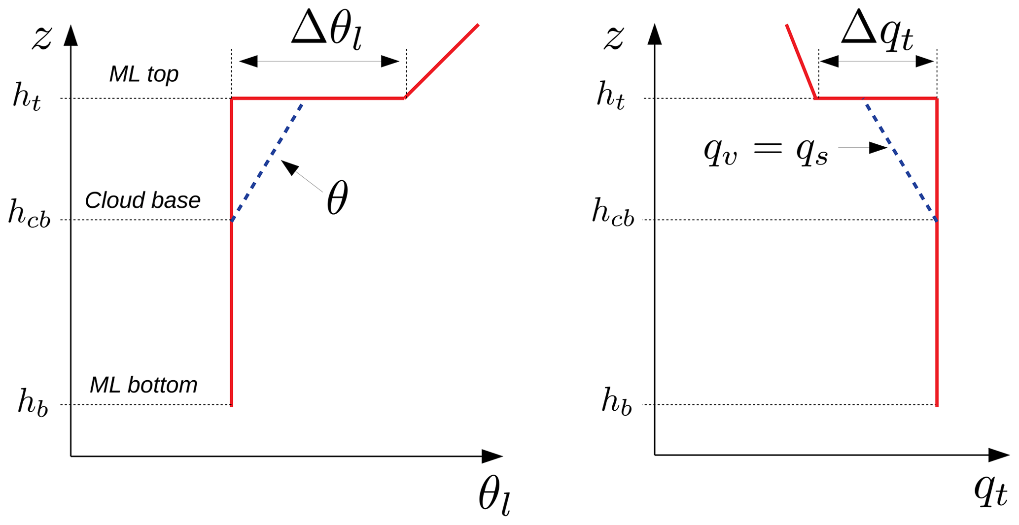
Figure C1 Schematic representation of the vertical profiles of the conserved variables θ_l and q_t in the mixed layer.

It is also useful to obtain a diagnostic relation for the virtual potential temperature flux $\stackrel{\mathrm{‾}}{w^{\prime }{\mathit{\theta }}_{\mathrm{v}}^{\prime }}$, which is associated with the buoyancy flux. If we neglect the small contribution of the liquid cloud water q_c to air density, the virtual potential flux is

$$\begin{array}{}\text{(C8)}& \stackrel{\mathrm{‾}}{w^{\prime }{\mathit{\theta }}_{\mathrm{v}}^{\prime }}=\stackrel{\mathrm{‾}}{w^{\prime }{\mathit{\theta }}^{\prime }}+\mathit{\theta }\left(\mathrm{1}+\mathrm{0.61}\stackrel{\mathrm{‾}}{w^{\prime }{q}_{\mathrm{v}}^{\prime }}\right).\end{array}$$

In the cloud layer we can use Eqs. (C6) in (C8) to obtain

$$\begin{array}{}\text{(C9)}& \stackrel{\mathrm{‾}}{w^{\prime }{\mathit{\theta }}_{\mathrm{v}}^{\prime }}=\stackrel{\mathrm{‾}}{w^{\prime }{\mathit{\theta }}^{\prime }}\left[\mathrm{1}+\mathrm{0.61}{q}_{\mathrm{s}}\left(\mathrm{1}+{\displaystyle \frac{L}{R_{\mathrm{v}}T}}\right)\right],\end{array}$$

while below the cloud layer

$$\begin{array}{}\text{(C10)}& \stackrel{\mathrm{‾}}{w^{\prime }{\mathit{\theta }}_{\mathrm{v}}^{\prime }}=\stackrel{\mathrm{‾}}{w^{\prime }{\mathit{\theta }}_{\mathrm{l}}^{\prime }}+\mathit{\theta }\left(\mathrm{1}+\mathrm{0.61}\stackrel{\mathrm{‾}}{w^{\prime }{q}_{\mathrm{t}}^{\prime }}\right).\end{array}$$

The turbulent entrainment fluxes ${\left.\stackrel{\mathrm{‾}}{w^{\prime }{\mathit{\theta }}_{\mathrm{l}}^{\prime }}\right|}_{z=h_{\mathrm{t}}}$ and ${\left.\stackrel{\mathrm{‾}}{w^{\prime }{q}_{\mathrm{t}}^{\prime }}\right|}_{z=h_{\mathrm{t}}}$ across the boundary-layer top are parameterized as

$$\begin{array}{}\text{(C11)}& {\displaystyle }{\left.\stackrel{\mathrm{‾}}{w^{\prime }{\mathit{\theta }}_{\mathrm{l}}^{\prime }}\right|}_{z=h_{\mathrm{t}}}=-w_{\mathrm{e}}\mathrm{\Delta }{\mathit{\theta }}_{\mathrm{l}},\text{(C12)}& {\displaystyle }{\left.\stackrel{\mathrm{‾}}{w^{\prime }{q}_{\mathrm{t}}^{\prime }}\right|}_{z=h_{\mathrm{t}}}=-w_{\mathrm{e}}\mathrm{\Delta }{q}_{\mathrm{t}},\end{array}$$

where $\mathrm{\Delta }{\mathit{\theta }}_{\mathrm{l}}=\mathrm{\Delta }\mathit{\theta }-L/c_p\mathrm{\Delta }{q}_{\mathrm{c}}$ and $\mathrm{\Delta }{q}_{\mathrm{t}}=\mathrm{\Delta }{q}_{\mathrm{v}}+\mathrm{\Delta }{q}_{\mathrm{c}}$ are the jumps of the conservative variables across the mixed-layer top. For the entrainment velocity, we use one of the most simple parameterizations, namely

$$\begin{array}{}\text{(C13)}& w_{\mathrm{e}}=A{\displaystyle \frac{{\mathit{\theta }}_{\mathrm{0}}}{g}}{\displaystyle \frac{w_{*}^{\mathrm{3}}}{\mathrm{\Delta }{\mathit{\theta }}_{\mathrm{v}}\mathrm{\Delta }h}},\end{array}$$

where A=0.2 is the typically used value of the proportionality constant. In Eq. (C13), we assume Δθ_v≈Δθ.

In the used parameterization of entrainment, similar to Randall (1980), we assume that all of the observed radiative flux divergence occurs in the turbulent cloudy layer.

Finally, following Deardorff (1980) and Nicholls (1989) we can use the diagnosed profile of the buoyancy flux to obtain the vertical velocity and temperature scales w_⋆ and θ_⋆, respectively, as

$$\begin{array}{}\text{(C14)}& {\displaystyle }{w}_{*}=(\mathrm{2.5}I{)}^{\mathrm{1}/\mathrm{3}},\text{(C15)}& {\displaystyle }{\mathit{\theta }}_{*}=w_{\star }^{\mathrm{2}}{\mathit{\theta }}_{\mathrm{v}}/gh,\end{array}$$

where

$$\begin{array}{}\text{(C16)}& I=(g/{\mathit{\theta }}_{\mathrm{0}})\underset{h_{\mathrm{bot}}}{\overset{h_{\mathrm{top}}}{\int }}\stackrel{\mathrm{‾}}{w^{\prime }{\mathit{\theta }}_{\mathrm{v}}^{\prime }}\mathrm{d}z.\end{array}$$

Furthermore, Eq. (C14) can be used to estimate the expected values of σ_w in the mixed layer. Namely, Lenschow et al. (1980) suggested the following parameterization for ${\mathit{\sigma }}_w/w_{*}$ as function of z, namely

$$\begin{array}{}\text{(C17)}& {\displaystyle \frac{{\mathit{\sigma }}_w^{\mathrm{2}}}{w_{*}^{\mathrm{2}}}}=c_{\mathrm{1}}{\left[{\displaystyle \frac{z_{\mathrm{top}}-z}{z_{\mathrm{top}}-z_{\mathrm{bot}}}}\right]}^{\mathrm{2}/\mathrm{3}}{\left[\mathrm{1}-c_{\mathrm{2}}{\displaystyle \frac{z_{\mathrm{top}}-z}{z_{\mathrm{top}}-z_{\mathrm{bot}}}}\right]}^{\mathrm{2}},\end{array}$$

where z_top and z_bot are the mixed-layer top and bottom heights, respectively; c₁=1.8 and c₂=0.8 are the empirical constants. Equation (C17) is valid for $z_{\mathrm{bot}}\le z<z_{\mathrm{top}}$.