the Creative Commons Attribution 4.0 License.
the Creative Commons Attribution 4.0 License.
 | 29 Mar 2023
Measurement report: Understanding the seasonal cycle of Southern Ocean aerosols
Ruhi S. Humphries
Melita D. Keywood
Jason P. Ward
James Harnwell
Simon P. Alexander
Andrew R. Klekociuk
Keiichiro Hara
Ian M. McRobert
Alain Protat
Joel Alroe
Luke T. Cravigan
Branka Miljevic
Zoran D. Ristovski
Robyn Schofield
Stephen R. Wilson
Connor J. Flynn
Gourihar R. Kulkarni
Gerald G. Mace
Greg M. McFarquhar
Scott D. Chambers
Alastair G. Williams
Alan D. Griffiths
The remoteness and extreme conditions of the Southern Ocean and Antarctic region have meant that observations in this region are rare, and typically restricted to summertime during research or resupply voyages. Observations of aerosols outside of the summer season are typically limited to long-term stations, such as Kennaook / Cape Grim (KCG; 40.7∘ S, 144.7∘ E), which is situated in the northern latitudes of the Southern Ocean, and Antarctic research stations, such as the Japanese operated Syowa (SYO; 69.0∘ S, 39.6∘ E). Measurements in the midlatitudes of the Southern Ocean are important, particularly in light of recent observations that highlighted the latitudinal gradient that exists across the region in summertime. Here we present 2 years (March 2016–March 2018) of observations from Macquarie Island (MQI; 54.5∘ S, 159.0∘ E) of aerosol (condensation nuclei larger than 10 nm, CN10) and cloud condensation nuclei (CCN at various supersaturations) concentrations. This important multi-year data set is characterised, and its features are compared with the long-term data sets from KCG and SYO together with those from recent, regionally relevant voyages. CN10 concentrations were the highest at KCG by a factor of ∼50 % across all non-winter seasons compared to the other two stations, which were similar (summer medians of 530, 426 and 468 cm−3 at KCG, MQI and SYO, respectively). In wintertime, seasonal minima at KCG and MQI were similar (142 and 152 cm−3, respectively), with SYO being distinctly lower (87 cm−3), likely the result of the reduction in sea spray aerosol generation due to the sea ice ocean cover around the site. CN10 seasonal maxima were observed at the stations at different times of year, with KCG and MQI exhibiting January maxima and SYO having a distinct February high. Comparison of CCN0.5 data between KCG and MQI showed similar overall trends with summertime maxima and wintertime minima; however, KCG exhibited slightly (∼10 %) higher concentrations in summer (medians of 158 and 145 cm−3, respectively), whereas KCG showed ∼40 % lower concentrations than MQI in winter (medians of 57 and 92 cm−3, respectively). Spatial and temporal trends in the data were analysed further by contrasting data to coincident observations that occurred aboard several voyages of the RSV Aurora Australis and the RV Investigator. Results from this study are important for validating and improving our models and highlight the heterogeneity of this pristine region and the need for further long-term observations that capture the seasonal cycles.
Please read the corrigendum first before continuing.
-
Notice on corrigendum
The requested paper has a corresponding corrigendum published. Please read the corrigendum first before downloading the article.
-
Article
(4257 KB)
-
The requested paper has a corresponding corrigendum published. Please read the corrigendum first before downloading the article.
- Article
(4257 KB) - Full-text XML
- Corrigendum
- BibTeX
- EndNote


Understanding the pre-industrial atmosphere is fundamental to characterising the impact of anthropogenic activity on the world's climate. Atmospheric time capsules such as ice cores have been pivotal in reconstructing the past variability of greenhouse gases and certain aerosol constituents. However, these proxies are not available for many aerosol properties. To gain an understanding of this baseline atmosphere, we need to measure a proxy atmosphere that is as near to being anthropogenic-free as is possible. While not entirely devoid of atmospheric pollution, the Southern Ocean and Antarctic region is one of the most remote regions, being far from both continental and urban influences, making it the best proxy we have to a pristine atmosphere. This makes it an important location to understand the pre-industrial atmosphere and the natural processes that occur here that are often masked by the much larger signals associated with anthropogenic activity (Carslaw et al., 2013; McCoy et al., 2020).
The most recent Intergovernmental Panel on Climate Change (IPCC) reports (IPCC, 2014, 2021) identified aerosol–cloud interactions as exhibiting the largest uncertainties in our understanding of the Earth's climate. A large driver for this are the natural background processes that can only be observed in pristine regions, as illustrated by the significant uncertainties and biases that exist in the simulation of clouds, aerosols and air–sea exchanges in climate and earth system models in the Southern Ocean region (e.g. Marchand et al., 2014; Shindell et al., 2013; Pierce and Adams, 2009). Importantly, these biases are driven by a poor understanding of the underlying physical processes occurring in the region, with impacts seen in our understanding of tropical rainfall distribution (Frey and Kay, 2018), the global energy budget (Trenberth and Fasullo, 2010), and our ability to model the impact of carbon-cycle and cloud feedbacks on climate change (IPCC, 2014; Gettelman et al., 2016).
Aerosols in this region are well known to be derived primarily from natural sources, including primary particles (sea spray and bubble bursting), which dominate the mass concentration, and secondary particles, which drive the number concentrations of both condensation nuclei (CN) and cloud condensation nuclei (CCN). Numerous observations (e.g. Shaw, 1988; Gras, 1983; Bigg et al., 1984; Kreidenweis et al., 1998; Bates et al., 1998; Covert et al., 1998; Quinn et al., 2000; Rinaldi et al., 2010, 2020; Frossard et al., 2014; Sanchez et al., 2021) have found that the secondary particles in the region originate from non-sea-salt sulfate, likely originating from the oxidation products of dimethyl sulfide (DMS) emitted from phytoplankton and sea ice algae, such as methanesulfonic acid (MSA) and sulfuric acid. Seasonal emissions of these aerosol precursor gases coincides with the significant seasonal cycles of phytoplankton populations (Lana et al., 2011), resulting in the typical annual cycles observed in aerosol populations in the region.
Phytoplankton abundance exhibits strong regional heterogeneity and latitudinal gradients, with the highest concentrations centred near the sea ice regions (Deppeler and Davidson, 2017). This spatial heterogeneity, combined with the atmospheric transport processes and timelines for chemical and physical generation and processing of aerosols, is likely to result in significant spatial heterogeneity in aerosol populations across the region that are of a similar magnitude but may not be well correlated with phytoplankton abundance.
Intensive field campaigns with aerosol observations have occurred only a handful of times throughout the last century (Bigg, 1990a; Bates et al., 1998; O'Dowd et al., 1997; Boers, 1995). However, in response to the recognition of the importance of the region to the climate and Earth system more widely, there has been a recent flurry of aerosol observations in the region, resulting in at least 16 aerosol inclusive campaigns between 2009 and 2018 (Wofsy, 2011; Law et al., 2017; Humphries et al., 2015, 2016; Dall'Osto et al., 2017; Fossum et al., 2018; Stephens et al., 2018; Schmale et al., 2019; Brock et al., 2019; Sato et al., 2018; McFarquhar et al., 2021; Mace and Protat, 2018; Mace et al., 2021; Alroe et al., 2020; Simmons et al., 2021; Sanchez et al., 2021; Twohy et al., 2021; Kremser et al., 2021), with at least another 20 more campaigns planned in the region before the end of 2025. Of particular note is the establishment of ongoing observations (as part of the World Meteorological Organisation's Global Atmosphere Watch, WMO-GAW, programme) aboard RV Investigator, based in Australia, and the soon to be online observations aboard the French owned RV Marion Dufresne II.
While ongoing observations are particularly important for characterising seasonal and long-term changes in the region, the challenges associated with ongoing operation in this environment make them few and far between. There have been many observational programmes incorporating aerosol microphysical measurements across the region that have spanned from a few weeks to many years (e.g. Asmi et al., 2010; Koponen et al., 2003; Kyrö et al., 2013; Claeys et al., 2010; Kubicki et al., 2016; Savoie and Prospero, 1989; Li et al., 2018; Schmale et al., 2013; Bigg et al., 1983; Gras, 1993; Pant et al., 2011; Hansen et al., 2009; Brechtel et al., 1998; Weller et al., 2018). Observational platforms that are currently in operation and present long-term records include those in the East Antarctic sector of the continent or in the Southern Ocean: i.e. Syowa (69.0∘ S, 39.0∘ W; e.g. Hara et al., 2011b) and Kennaook / Cape Grim (40.7∘ S, 144.7∘ E; e.g. Gras and Keywood, 2017); those in the West Antarctic sector, i.e. Neumayer (70.67∘ S, 8.27∘ W; e.g. Weller et al., 2015, 2011), King Sejong Station (62.22∘ S, 58.78∘ W; e.g. Hong et al., 2020; Jang et al., 2022) and Princess Elisabeth Station (71.95∘ S, 23.35∘ E; e.g. Herenz et al., 2019); and South Pole (0∘ E, 90∘ S; e.g. Park et al., 2004). While this list might sound long, many of these observations are patchy over the many decades since this technology has been viable, and with only five stations undertaking ongoing continuous observations over such a large and heterogeneous spatial area, it is striking how few data exist in a region that is so important for both the regional and global climate.
In this study, we focus primarily on observations in the East Antarctic region, presenting newly acquired data from Macquarie Island and contrasting these observations with those from nearby East Antarctic observations at long-term stations (i.e. Kennaook / Cape Grim and Syowa) as well as numerous recent ship voyages in the region. Observations of aerosol properties at Macquarie Island have occurred previously during the ACE 1 campaign for approximately 3 weeks in the late spring to early summer of 1995 (Brechtel et al., 1998; Kreidenweis et al., 1998). These represent valuable observations and had important results including that aerosol properties depended largely on the air mass origin, with influences from both Antarctica and Tasmania, as well as clean marine air originating over the Southern Ocean. This study builds on that short campaign and extends previous work undertaken characterising the seasonal changes in Southern Ocean aerosol populations (e.g. Gras and Keywood, 2017; Weller et al., 2011; Bigg et al., 1983; Gras, 1993, 1990; Hara et al., 2011b; Kim et al., 2017) as well as further expanding on work undertaken by Alroe et al. (2020) and Humphries et al. (2021a) in understanding the latitudinal changes observed across this region. In particular, this work takes both seasonal station data and voyage data to develop an understanding of both seasonal and latitudinal variability across the East Antarctic sector of the Southern Ocean region.
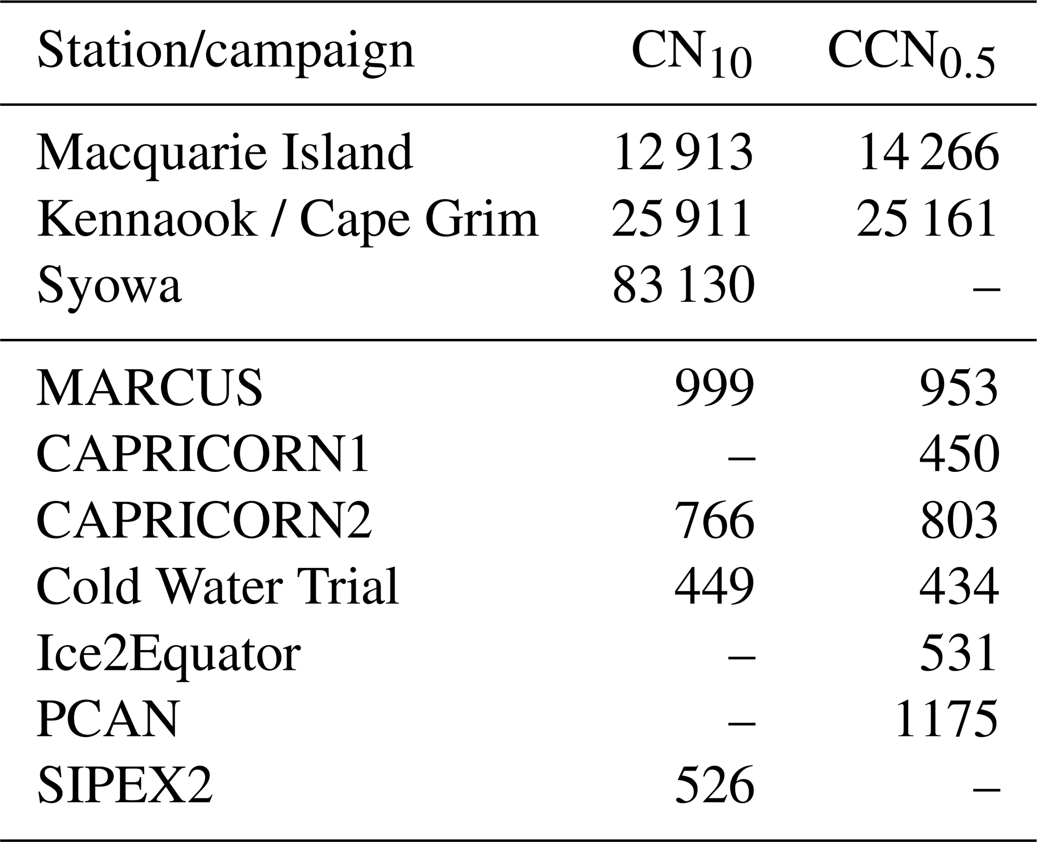
Two years of observations of CN10 and CCN were made at the Australian sub-Antarctic research station located on Macquarie Island in the midlatitudes of the Southern Ocean (54.5∘ S, 159.0∘ E). To support the analysis of these data and to give greater spatial and temporal context to the data set, observations from a number of other long-term stations and campaigns are utilised in this study. Figure 1 shows the locations of these observations. Aerosol data from three ground-based stations are included: Macquarie Island, Kennaook / Cape Grim (40.7∘ S, 144.7∘ E) and Syowa (69.0∘ S, 39.0∘ E). In addition, data from a range of intensive observational campaigns aboard two research vessels, the RSV Aurora Australis and the RV Investigator, have been utilised and are detailed below. Each of these data sets are quality controlled in ways that are particular to their location and platform, the details of which are outlined below. The resulting number of hourly observations of clean data utilised in this study are summarised in Table 1.
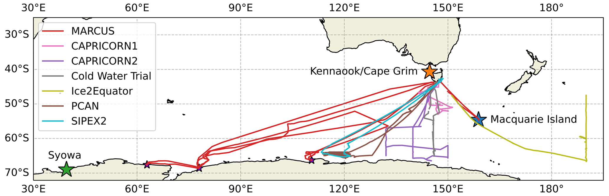
Figure 1Map showing the relative locations of the three long-term stations utilised in this study: Kennaook / Cape Grim (40.7∘ S, 144.7∘ E), Macquarie Island (54.5∘ S, 159.0∘ E) and Syowa (69.0∘ S, 39.6∘ E). Voyage tracks of those voyages utilised in this study are also shown. Both SIPEX2 and MARCUS occurred aboard ice breaker RSV Aurora Australis, with the latter occurring throughout a full season of four resupply voyages to Australian Antarctic stations (from west to east: Mawson, Davis, Casey (all shown as black stars) and (labelled) Macquarie Island). Note that data from the Ice2Equator voyage have been sub-selected (>47.5∘ S) for those likely to be representative of Southern Ocean air masses unaffected by New Zealand continental influence or tropical air further north.
Table 1Number of hourly observations available from each station or voyage after quality control.
2.1 Macquarie Island
Macquarie Island (MQI) is a small, isolated island (34 km long and up to 5 km wide) oriented approximately north–south in the Southern Ocean. A comprehensive site description is provided separately by Stavert et al. (2019). Aerosol observations at MQI were made in the Clean-Air Laboratory, located on an isthmus near the northern tip of the island, and upwind (westward) of the adjacent permanently occupied research station. The observational programme ran as part of the MICRE (Macquarie Island Cloud and Radiation Experiment) and ACRE (Antarctic Clouds and Radiation Experiment) projects from March 2016 to March 2018 (McFarquhar et al., 2021; Tansey et al., 2022). Together these projects deployed a suite of instrumentation including cloud lidars and radars, a distrometer, a range of radiometers, and, most relevant to the current study, in situ aerosol samplers measuring condensation nuclei (CN) and cloud condensation nuclei (CCN) number concentrations. All CN and CCN data from this project are available at Humphries et al. (2021c).
2.1.1 Condensation nuclei
Number concentrations of condensation nuclei (aerosols) larger than 10 nm (CN10) were measured continuously at 1 Hz using a condensation particle counter (CPC model 3772, TSI Inc. Shoreview, MN, USA). As is the case with all TSI CPCs, the CPC draws sample air continuously at a pre-defined flow rate through a chamber where the air is supersaturated with 1-butanol, providing an environment where the vapour will condense onto aerosols as small as 10 nm (with default manufacturer's settings for this model), growing them to supermicron sizes where they are counted individually using a simple optical particle counter. The instrument comes pre-installed from the factory with an internal critical orifice to maintain the nominal flow rate at 1.0 L min−1. However in marine environments, this critical orifice can block with sea salt and requires regular cleaning to prevent flow rate drift outside acceptable limits. Given the remote operation of these instruments, the CPC was reconfigured by replacing the critical orifice with an active mass flow controller (MFC; Alicat Scientific Model MC 5LPM) set to 1.0 L min−1. The MFC was calibrated in situ using an external low-pressure drop flowmeter (Sensidyne Gilibrator, St. Petersburg, FL, USA) placed in front of the CPC. MFC data were captured via the analogue input of the CPC for logging. Data from the CPC were filtered for periods of instrument zeros, flow checks, and other maintenance and outages (major outages detailed below). Once a clean data set was obtained, hourly statistics were calculated for the full multi-year data set.
There were two significant periods where data were removed. The first occurred from the start of measurements in March 2016 up until 16 June 2016 where the nozzle pressure increased slowly out of instrument specification due to sea salt aerosol build-up in the nozzle. While nozzle cleaning was already part of the scheduled maintenance, the build-up occurred much faster than anticipated. This resulted in a noticeable artefact in the CCN CN ratio that ended up being well above 1 (at its worst). All data were removed during this period and it was verified that this issue did not reoccur during the remainder of the campaign. The second issue occurred due to issues with the synchronisation with the time server. While it was possible to recover much of these data appropriately, data from 2 June to 21 July 2017 were too far out of sync with real time and were removed from the data set.
2.1.2 Cloud condensation nuclei
Number concentrations of CCN were measured continuously at 1 Hz at a range of supersaturations for the entire 2 years of observations using a continuous-flow, streamwise thermal-gradient CCN counter (CCNC; model CCN-100, Droplet Measurement Technologies, Longmont, CO, USA). Because of logistical constraints preventing scientific experts visiting the island for annual calibrations, the instrument was swapped out by onsite technicians after 1 year for a model that had been recently serviced and calibrated by the manufacturer. While instrument intercomparison could not be undertaken for this project, ongoing intercomparison of different instruments of the same model at Kennaook / Cape Grim have shown good agreement between instruments. The instrument was initially configured to run at 0.5 % supersaturation for 23 h of the day and then, in the remaining hour, to move sequentially through a full set of six supersaturations (10 min at each), including (in order) 1.0 %, 0.8 %, 0.6 %, 0.5 %, 0.4 % and 0.2 %. On 2 November 2016, this sampling pattern was altered so that it would scan through the supersaturation sequence every hour of the day.
Calibration of the supersaturation settings of both instruments deployed during ACRE was undertaken at the Droplet Measurement Technologies workshop in Boulder, Colorado, which is at a significant altitude above sea level (1620 m above sea level, 830 mbar). A supersaturation pressure correction was applied, resulting in actual measured supersaturations being 0.055 % higher than set points (e.g. 0.2 % was actually 0.255 %). Although a range of supersaturations were measured during this campaign (stated above), because of the need to compare observations with other sites where often only 0.5 % supersaturation was measured, this study focuses largely on this supersaturation. It is important to note though that a number of recent studies (Fossum et al., 2018; Sanchez et al., 2021; Twohy et al., 2021) have suggested that 0.3 % is likely to be the most representative of actual environmental conditions in this region.
Data were thoroughly quality controlled. The first 3 min of each 10 min period were removed to allow for the stabilisation of instrument conditions. Remaining data were screened for periods when instrument parameters were out of manufacturer specification, instrument maintenance and other outages. After this quality control, hourly statistics were calculated for each supersaturation (i.e. the maximum of 7 min of observations at each supersaturation was utilised to calculate statistics). One major instrument malfunction occurred during the campaign: the internal Nafion membrane that provides the essential supersaturation conditions within the instrument rapidly degraded over a period of about 7 weeks. This resulted in the removal of data from 25 April until 17 July 2017, at which point the Nafion was replaced.
Another major quality control issue arose because the CPU clock housed within the embedded PC of the CCNC exhibited significant time drift. Although time syncing with server time was performed weekly (and increased to daily after identification of this issue), the magnitude of the time drift was such that it still presented a major issue. Since the CCN population is a subset of the CN population, many features were observable in both data sets, allowing quantification of the time drift through comparison of the two time series. Unfortunately, this comparison revealed that the time offset drifted both forward and backward in time and could not be corrected for. Data were removed entirely when this drift became significant (greater than 2 min d−1), as occurred between the 19 and 25 August 2017. With the remaining data set, there were seven distinct periods where the time drift was different and highly variable, and this varied from 4.5 min slow to 3.25 min fast. Because the goal was to produce hourly statistics for these data, it was decided (after numerous failed attempts to align the data with various mathematical methods) that data at the start and end of each hour would be removed prior to resampling to hourly statistics. This ensured that the time drifting issue had no affect on resampled data.
2.1.3 Sampling system
Sample air was drawn into the Clean-Air Laboratory through a sample inlet positioned 1.5 m above the roofline (∼4 m above ground level, 10 m above sea level). The sample line was a bespoke design with a TSP (total suspended particles) weather hat mounted atop a vertical 3" o.d. stainless tubing, which provided both protection and vertical stability in the high wind environment. Through a bored-out Swagelok bulkhead fitting, a o.d. stainless steel tube penetrated through the external 3" o.d. tube to the height of the weather hat. The weather hat had three tie-down holes for guy wires to be attached for stabilisation to the laboratory roof. The top 1 m of the inlet, together with the weather hat were heated continuously to prevent icing with self-regulating heater tape designed to prevent ice build-up on commercial walk-in freezer doors. Heater tape was covered in insulation, followed by weather and UV-proof heat shrink.
The tubing that penetrated through the roof was connected inside the lab to a PM2.5 cyclone (URG Corp, Chapel Hill, NC, USA), with a sample flow rate of 16.67 L min−1. Both the CCNC and CPC sampled air at flow rates of 0.5 and 1.0 L min−1, respectively. In addition, there was a bypass flow of 15.1 L min−1 set by a variable area flow meter. Before the CCNC, a buffer volume was attached off the side of a T piece to help dampen pressure fluctuations caused by outside wind moving across the inlet, which the instrument can be sensitive to. To prevent water contamination of the 1-butanol working fluid, the sample was dried prior to entering the CPC using a Nafion drier (Nafion Drier model MD-110-12S-4, Perma Pure LLC, Lakewood, NJ, USA) setup using the differential pressure configuration with 1 L min−1 sample flow (defined by the CPC's MFC) and 5 L min−1 of HEPA-filtered laboratory air as sheath flow (defined by a rotameter).
2.2 Kennaook / Cape Grim
The Kennaook / Cape Grim (KCG) baseline atmospheric programme is one of three premier global stations of the WMO-GAW programme. The observatory is located at the north-west tip of Tasmania (40∘41′ S, 144∘41′ E) atop a cliff, sampling 94 m above sea level. The location enables the observation of Southern Ocean air that has had minimal recent anthropogenic influence. Air sampled in the “baseline” sector (190–280∘) has typically spent the previous several thousand kilometres without contact with land. Previously known as Cape Grim, the Indigenous heritage of the area has recently been recognised by the adoption of a dual-naming convention. With enthusiastic support from the community and station staff and scientists, the station is now known as Kennaook / Cape Grim.
Aerosol measurements at KCG have been occurring since the mid-1970s with a range of technologies and have followed what have now been established as WMO-GAW Aerosol Programme recommendations. In this study, data between 2010 and 2020 (inclusive) have been utilised for both CN10 (CPC model 3010, TSI Inc. Shoreview, MN, USA) and CCN0.5 (model CCN-100, Droplet Measurement Technologies, Longmont, CO, USA). The most recent analysis of these long-term data sets, along with further details of the measurements, is provided by Gras and Keywood (2017). Hourly median concentration data (CCN and CN10) are available in the World Data Centre for Aerosols (http://www.gaw-wdca.org/, last access: 1 July 2022). Note that only data from the baseline sector are used in this study to ensure air from the continent and anthropogenic regions is kept to a minimum. The baseline sector here is defined as periods with wind directions between 190 and 280∘ as well as radon concentrations below 100 mBq. We note that baseline air at KCG is observed between 15 %–35 % of the time, with the maximum occurring in austral winter (hence the lower number of observations shown in Table 1 for KCG relative to Syowa).
2.3 Syowa
Syowa Station (SYO) is located on East Ongul Island in Lützow-Holm Bay in East Antarctica (69.0∘ S, 39.0∘ E). The coastal station is surrounded by extensive sea ice throughout the year, extending approximately 100 km from the coast in summer and 1000 km in the winter–spring period. Comprehensive details of the station and the aerosol programme are provided in previous publications (e.g. Hara et al., 2011b, a).
Observations of aerosol number concentrations have been made continuously at SYO since 1997 using multiple CPCs (the long-term record has utilised CPC model 3010, TSI Inc. Shoreview, MN, USA). In 2004, a new clean-air observatory was built at the station to replace the ageing observatory. Simultaneous measurements were undertaken in both observatories (using the same TSI model 3010 CPC) during the 2004 period to ensure continuity of the record. While agreement is good between the records, the aerosol inlet in the new clean-air observatory is better designed. For the purposes of the current study, only ∼10 years of data were desired to enable a climatological comparison with the MQI data. Consequently, only data available from the new clean-air laboratory were utilised in this study, which included data from 2004 to 2016. All data are publicly available in Hara (2023).
2.4 Voyages aboard the RSV Aurora Australis
The RSV Aurora Australis (retired in 2020) was Australia's flagship ice breaker designed to undertake both marine science and station resupply voyages to the Antarctic continent. The vessel had no dedicated atmospheric composition observational capability, and, consequently, instrumentation was installed for specific campaigns, including full inlet systems.
2.4.1 MARCUS
The MARCUS (Measurements of Aerosols, Radiation and CloUds over the Southern Oceans) campaign occurred as a project aboard the RSV Aurora Australis during its summer resupply of Australia's Antarctic research stations between October 2017 and March 2018 (McFarquhar et al., 2021; Alexander and Klekociuk, 2021). Full details of the campaign have been published separately (Humphries et al., 2021a). In short, the campaign utilised the United States Department of Energy (DOE) Atmospheric Radiation Measurement (ARM) Program Mobile Facility 2 (AMF2). Cloud, radiation and precipitation instruments were deployed, along with the Aerosol Observing System (AOS) (https://www.arm.gov/capabilities/instruments/aos, last access: 1 July 2022). Utilised in this study are the CN10 (CPC model 3772, TSI Inc. Shoreview, MN, USA) and CCN observations (model CCN-100, Droplet Measurement Technologies, Longmont, CO, USA). Note that because of the lack of dedicated inlet systems for air sampling, campaign-specific systems were installed and, due to operational limitations, were located directly adjacent to the ship's own exhaust. This meant that this data set was heavily contaminated by the platform's own diesel exhaust, and consequently just over 10 % from the campaign was deemed usable (Humphries et al., 2021a). Exhaust-free aerosol data from the MARCUS campaign are available at Humphries (2020), with raw data available at the ARM archive (references within Humphries, 2020).
2.4.2 SIPEXII
The second Sea Ice Physics and Ecosystems eXperiment (SIPEXII) occurred from 14 September to 11 November in 2012. The 52 d marine science voyage travelled from its home port in Hobart to the East Antarctic pack ice between 112 and 122∘ E, during which time it set up eight temporary research stations atop ice floes (1–5 d periods anchored to the drifting ice floe). Full details of atmospheric observations during SIPEXII are found in earlier publications (Humphries et al., 2015, 2016). Aerosol measurements were limited to in situ aerosol number concentrations using two concentration particle counters (CPCs) with different size cuts of particles larger than 3 nm (CN3; model 3025A, TSI, Shoreview, MN, USA) and 10 nm (CN10; model 3772, TSI, Shoreview, MN, USA). SIPEXII data are incorporated in this study to compare with the MQI observations, and, consequently, only CN10 data are utilised here. Aerosol data from SIPEXII can be found at Humphries et al. (2014). Aerosol inlets for this voyage were able to be located further from the platform's exhaust compared with MARCUS, resulting in a greater percentage of data that were deemed usable due to contamination from the exhaust.
2.5 Voyages aboard the RV Investigator
The RV Investigator is Australia's flagship blue-water research vessel. Its home port is in Hobart, and since its commissioning in 2015, it has spent about two-thirds of its research voyage time in the Southern Ocean. It has two dedicated atmospheric laboratories, home to a suite of instrumentation for the measurement of aerosols, reactive gases and greenhouse gases. These instruments operate continuously throughout the year and have resulted in the platform being recognised as the first mobile platform of the WMO-GAW programme in 2018. Further details of the platform are provided in Humphries et al. (2019). Unfortunately, the data from all voyages of the RV Investigator are still being quality controlled, with all data from 2015 to 2021 (inclusive) expected to be published in the near future. Data from selected voyages, however, are already available, and those data sets utilised in this study are outlined below.
Unlike the RSV Aurora Australis, the RV Investigator's atmospheric laboratories are connected to a purpose-built air sampling inlet. This inlet is situated at the fore of the vessel, approximately 18 m above sea level, and is as far away from the ship's exhaust stack as is possible on the vessel. This scenario, combined with the different operational constraints of the vessel (i.e. greater freedom to align the vessel with its nose into the wind rather than orienting it to suit the ice conditions, as was often the case for the RSV Aurora Australis), means that contamination of atmospheric data by platform exhaust is much lower on the RV Investigator compared with the RSV Aurora Australis. Typically, exhaust contamination aboard the RV Investigator ranges between 10 %–50 % of the time.
2.5.1 Cold Water Trial
The Cold Water Trial voyage (voyage ID: IN2015_E01) occurred between 29 January and 17 February 2015. This voyage was the first voyage of RV Investigator into polar waters, and occurred during its commissioning phase. The voyage travelled south along the 146th line of longitude, reaching the Antarctic ice edge at approximately 65∘ S. A comprehensive analysis of these data is provided by Alroe et al. (2020). Both CN10 (model 3772, TSI, Shoreview, MN, USA) and CCN0.5 (model CCN-100, Droplet Measurement Technologies, Longmont, CO, USA) are available and were utilised for the current study. All data are available at Humphries et al. (2022b).
2.5.2 CAPRICORN1
The CAPRICORN (Clouds, Aerosols, Precipitation, Radiation, and atmospheric Composition Over the southeRn oceaN) campaign occurred aboard the RV Investigator between 14 March and 16 April 2016 (part of IN2016_V02; Mace and Protat, 2018). The voyage departed Hobart and spent its time undertaking a range of marine characterisation and sampling down to 53∘ S, due south of Hobart. The campaign deployed a full suite of instrumentation; however, included here is just CCN concentration measured at 0.5 % supersaturation (model CCN-100, Droplet Measurement Technologies, Longmont, CO, USA). Data are publicly available at Protat and Humphries (2020).
2.5.3 Ice2Equator
The Ice2Equator campaign occurred as part of the IN2016_V03 voyage, directly after the CAPRICORN1 voyage, between 25 April and 30 June 2016. The voyage travelled south-east from Hobart to the Antarctic ice edge (66.7∘ S) before heading north along the 170∘ W longitude line to the Equator. The voyage concluded in Lautoka, Fiji, and also had a mid-voyage stopover in Wellington, New Zealand, for personnel change-over. Full details of the voyage and results from its atmospheric analysis are provided in the PhD thesis of Alroe (2021) and are expected to be published in a peer-reviewed journal in the near future. Because the focus of the current study is just on background Southern Ocean air, data from this voyage have been limited to only those south of 47.5∘ S in order to both keep data representative of Southern Ocean air masses and ensure we avoid continental influence during periods downwind of New Zealand. CCN0.5 concentrations (model CCN-100, Droplet Measurement Technologies, Longmont, CO, USA) have been utilised in this study. All data are available at Humphries et al. (2022a).
2.5.4 PCAN
The Polar Cell Aerosol Nucleation (PCAN) campaign occurred as part of the IN2017_V01 voyage between 14 January and 4 March 2017. The voyage departed Hobart, traversing south-west across the Southern Ocean before spending most of its time (40 d) in the study area south of 60∘ S and between 110 and 120∘ E. Because one of the primary goals of the voyage was mapping the seafloor in the study area, a “mowing-the-lawn” pattern was adopted, which increased the impact of sampling platform exhaust, resulting in higher than usual exhaust contamination in these data. Despite this, data are still valuable and CCN concentrations (model CCN-100, Droplet Measurement Technologies, Longmont, CO, USA) at a range of supersaturations have been utilised in this study. Full details and analysis of the voyage data are provided in Simmons et al. (2021), and data are available at Humphries et al. (2020).
2.5.5 CAPRICORN2
The second CAPRICORN campaign occurred between 11 January and 21 February 2018 (part of IN2018_V01) and ventured all the way to the Antarctic ice edge. Data from this voyage have been published previously in Humphries et al. (2021a). As in CAPRICORN1, a range of instrumentation was deployed; however, we have limited our analysis here to those consistent with MQI observations, i.e. CN10 (model 3772, TSI, Shoreview, MN, USA) and CCN (model CCN-100, Droplet Measurement Technologies, Longmont, CO, USA) at various supersaturations. These data are available at Humphries et al. (2021b).
The full time series of CN10 and CCN0.5 from MQI is show in Fig. 2a. Consistent with previous observations in this region (e.g. Bigg, 1990b; Gras and Keywood, 2017), concentrations were observed to be very low (relative to other marine environments), exhibiting summer maxima and winter minima (shown in Fig. 2b and c). The hourly resolution time series shows significant short-term spikes, many of which coincide with winds from the northerly direction (270–90∘). Interestingly, the local research station is located directly north-east of the clean-air observatory and, consequently, may only be able to explain a small percentage of the large excursions in the data. Given the majority of these spikes are not from local sources, it is reasonable to suggest that these events are likely the result of long-range transport from continental air masses leaving mainland Australia. Correlation plots (not shown) of CN and CCN standard deviations with radon concentrations reveal that while some of this variability can be explained by continental influence, most of the data, including the high aerosol concentrations, occur when radon concentrations are below 150 mBq, which is reflective of maritime air.
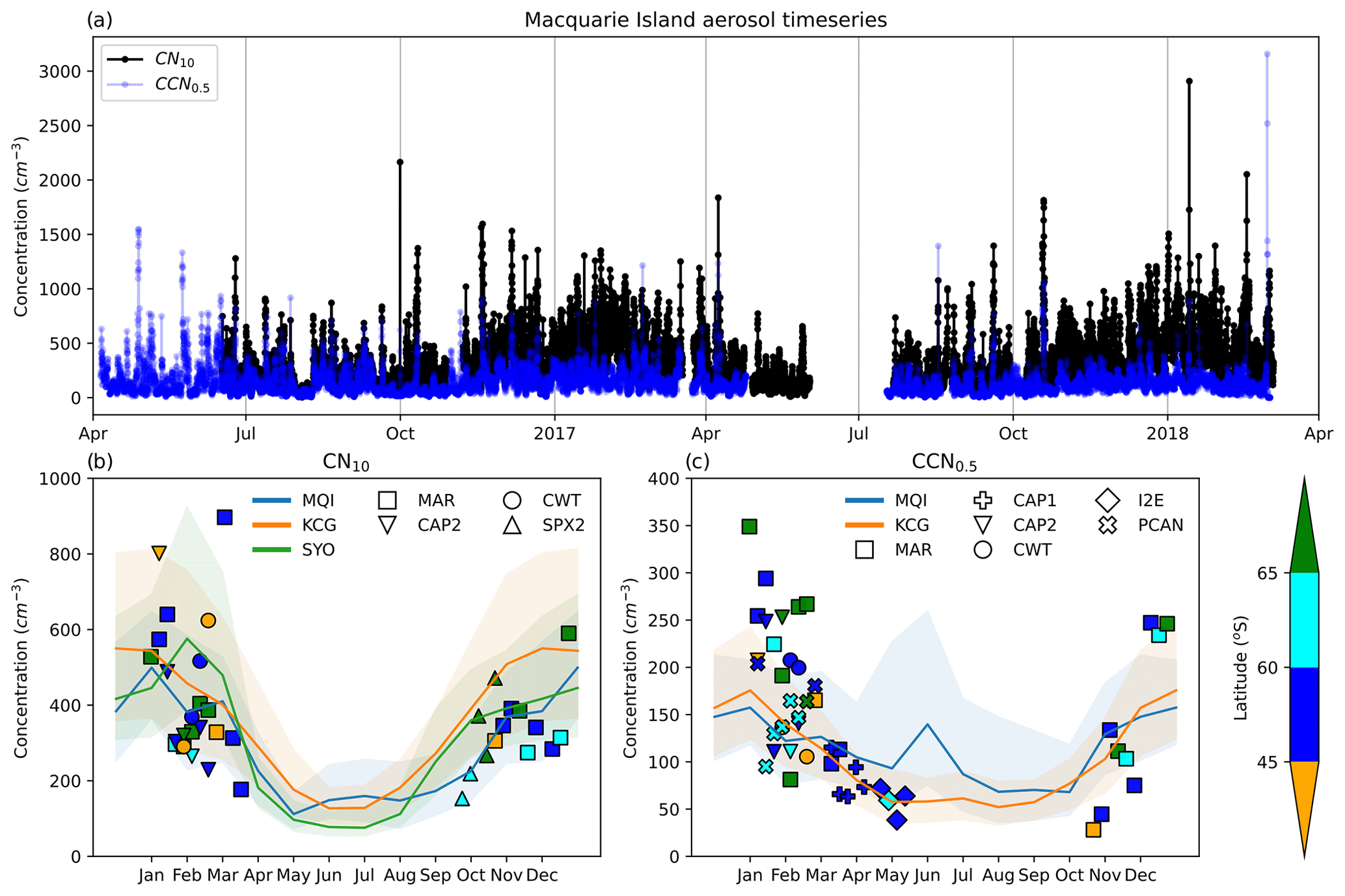
Figure 2The full time series (a) of hourly median aerosol observations (only showing CN10 and CCN0.5) from Macquarie Island between April 2016 to March 2018. Seasonal cycles of CN10 (b) and CCN0.5 (c) from Macquarie Island (MQI, 2016–2018), Kennaook / Cape Grim (KCG, 2011–2020) and Syowa (SYO, 2004–2016) are shown, with monthly medians (solid line) and interquartile range (shaded regions) shown. Overlaid on the seasonal cycles are the weekly medians from ship-based campaigns coloured by latitudinal bins. Note the y scale of (c) has been adjusted to highlight the seasonal cycle, but this excludes a data point from MARCUS in March showing a weekly CCN0.5 median concentration of 586 cm−3 corresponding to the CN10 data point of 897 cm−3 in (b).
3.1 CN10 seasonal cycles
Figure 2b shows the seasonal cycle of CN10 from MQI alongside those from KCG and SYO. Note that the seasonal cycle is plotted over 18 months to show the maxima and minima clearly, as presented in Appendix Fig. A1a. Summertime maxima are observed for all three stations, with the highest concentrations observed at the northernmost station, KCG, for most of the year. SYO exhibits summertime concentrations of a similar magnitude to KCG; however, the timing of the maxima is offset by 1 month, peaking in February, as compared with the other two stations, which peak in January. It is worth noting that this pattern, of SYO's maxima occurring 1 month later than northern locations, is consistent even when looking at individual years (not shown). While the timing of the summertime maxima are the same for MQI and KCG, the concentrations observed at the latter are 10 %–40 % higher. Concentrations at MQI and SYO remain high until a sudden drop in April before their winter minima begin in May. In contrast, KCG concentrations begin declining immediately after the January peak but make a more steady decline to reach the winter minima in June. Springtime increases begin almost simultaneously in August at both KCG and SYO, while the increase at MQI is delayed by about 2 months. Overall there is good agreement between concentrations observed at SYO and MQI, with the exception of the high late summer concentrations observed at SYO but absent at MQI.
The source of aerosols in this region is primarily wind-driven sea salt and secondary aerosol formation from the oxidation of biological emissions (e.g. Bigg et al., 1984; Ayers and Gras, 1991; Jimi et al., 2007; Gras and Keywood, 2017, and references therein). It is this latter source which is generally accepted to be the primary driver of the aerosol seasonal cycle in the Southern Ocean and Antarctic region. Around Antarctica in particular, the cold water and abundant marine nutrients serve as ideal breeding grounds for large communities of phytoplankton, which are known to reach their maximum abundance in late summer (Deppeler and Davidson, 2017). While still present at lower latitudes, these phytoplankton communities are less abundant. In addition, sea ice algae build up over winter at the higher latitudes and release their emissions during the melting season in spring and summer (e.g. Jang et al., 2022). These spatial and temporal differences between the Southern Ocean stations of KCG and MQI, compared with the Antarctic station, go a long way to explain the differences in timing and magnitude of the summertime maxima.
Also at play here is the air mass transport pathways influencing the different stations. Previous studies (Humphries et al., 2016, 2021a; Alroe et al., 2020; Simmons et al., 2021; Chambers et al., 2018) have established that a distinct atmospheric compositional boundary exists, known as the Atmospheric Compositional Front of Antarctica (ACFA), that is typically found between 60 and 65∘ S in the East Antarctic sea ice region. The ACFA has been found to reduce the flow of air between the higher and lower latitudes (Humphries et al., 2016). In particular, emissions from phytoplankton communities around the Antarctic coastline in summer tend to not be homogeneously mixed throughout the Southern Ocean atmosphere and, instead, influence the Antarctic continent more so, leading to the differences observed in aerosol concentrations between stations in this study.
Further to the above, the delayed increase in concentrations observed at MQI relative to the other two stations is likely the result of the lower abundance of phytoplankton communities and the absence of sea ice algal communities, at the latitudes at which Macquarie Island is situated. Phytoplankton communities are found (Deppeler and Davidson, 2017) to congregate more around coastlines where upwelling of nutrients occurs more frequently than in the open ocean (i.e. at MQI latitudes). This results in higher precursor emissions at these latitudes, leading to secondary particle formation and a rapid increase in concentrations at the stations closer to larger landmasses (i.e. KCG and SYO). It is plausible that the delayed increase in concentrations at MQI is a result of the delayed increase in phytoplankton populations in the open ocean together with the increased time required for cross-latitudinal air mass mixing to occur.
The wintertime minimum in SYO is noticeably lower than those of the other two stations. In wintertime in the Southern Ocean and Antarctic region, the biological driver of aerosols is largely absent, and aerosol concentrations are driven primarily by wind-driven sea salt. While all three stations are on the coastline surrounded by water, SYO is unique in that its surrounding ocean is covered in sea ice all year round, with its wintertime extent reaching approximately 1000 km. This results in a significant reduction in the ability of high winds to produce sea salt aerosol and is the likely explanation of the wintertime differences observed between the three stations.
The differences observed between MQI and KCG are worth noting. Both stations are in the Southern Ocean; however, the CN10 concentrations observed at KCG are higher than those observed at MQI throughout the year (with the exception of midwinter), reaching up to double the concentrations during some periods. KCG has long been thought of as being representative of the Southern Ocean region in general. While true for many atmospheric species, a recent study analysing data from MARCUS and CAPRICORN2 (Humphries et al., 2021a) showed that summertime aerosol concentrations were substantially higher than those at higher latitudes, with observations at KCG representative only of voyage observations north of 45∘ S. A voyage will take place in 2025, one goal of which is to experimentally answer the question of how representative observations at KCG are of the wider Southern Ocean. It may be the case that the region north of 45∘ S is somewhat distinct from the higher latitudes and the drivers of this difference should be investigated further.
Weekly voyage CN10 medians are shown overlaid on station seasonal cycles in Fig. 2b and are coloured by latitudinal bands. These bands have been chosen based on results of Humphries et al. (2021a) where the region exhibits different aerosol populations across three primary sectors: the area north of 45∘ S, Southern Ocean midlatitudes from 45 to 65∘ S and the area south of 65∘ S. Humphries et al. (2021a) established these divisions based on summertime voyage data split into 5∘ latitudinal bins; however, it is known that the ACFA varies latitudinally with time, and its position is likely to vary significantly with season, similar to the oceanic polar front (Seidel et al., 2008; Lucas et al., 2014; Davis and Rosenlof, 2012; Choi et al., 2014). Unpublished data from the summer CAPRICORN2 voyage show that the position can vary several degrees in a short time span and by longitude: the ACFA was observed at around 63∘ S, 140∘ E and a week later at 65∘ S, 150∘ E. The springtime SIPEXII voyage observed the ACFA at 64.4∘ S, 140∘ E. Unfortunately, data outside of summer in this latitudinal band are very limited, so thorough characterisation of the seasonal location is impossible with currently available data sets. This variability, together with the likely larger variability associated with seasonal changes, has led the authors to establish a fourth latitudinal band for this analysis, from 60 to 65∘ S, where data are available.
Overall, voyage data appear to agree well with long-term seasonal data sets. Since most of the voyages occurred south of Tasmania, only limited data are available for the northern sector (orange markers in Figs. 2b, c). These data all fall within the ranges of those observed at KCG. Similarly, voyage data from the midlatitudes (blue markers) agree well with data measured at MQI, with the exception of a single week in March which was anomalously high and was likely a result of measuring outflow from Tasmania (this was measured during MARCUS approximately halfway between Hobart and MQI). Voyage data in the polar cell sector (green markers) agree well with SYO concentrations throughout the year, except for during the February maximum at SYO, where voyage data are below SYO's 25th percentile. This could be a result of longitudinal variability, since Syowa is a long distance west of where these voyage data were obtained. The transitional sector between 60 and 65∘ S (cyan markers) is found to largely be on the lower end of the seasonal distributions and is observed to typically be consistent with midlatitude Southern Ocean CN10 data.
3.2 CCN seasonal cycles
The seasonal cycle of CCN0.5 is shown in Fig. 2c for platforms where those data are available (18-month version found in Appendix Fig. A1b). Unfortunately, CCN data were unavailable at SYO. As expected, the overall pattern of the CCN seasonal cycle follows that of CN for each site, with a typical summer maximum and winter minimum. For both KCG and MQI where seasonal CCN data are available, the summer maxima occurs in January, consistent with CN observations at the same sites. For KCG, CCN data reach their minimum in May, remaining at approximately the same minimum value until they start to rise in October. This is in contrast to the CN minimum, which only reaches its minimum in June and July. At KCG then, the increase in CCN over the warmer months occurs over a much narrower time period than does the CN: 7 months above background compared with 10. It could be that this pattern is a result of insufficient precursor gases (i.e. oxidation products of biological emissions such as DMS and MSA) in the shoulder seasons resulting in aerosol populations at sizes too small to be able to act as CCN. This is an interesting question and should be investigated further looking at multi-year time series of aerosol size distributions. While routine observations of aerosol size distributions have recently begun at KCG, data are not yet available for comprehensive analysis and will be a topic of future work.
The most surprising characteristic of the available seasonal cycles is the significant spike in CCN0.5 concentrations at MQI, beginning in May and peaking in June. This feature, present at all supersaturations (Appendix Fig. A2), is of the same magnitude as the summer maximum in CCN but, interestingly, is not one that is observed in the CN10 data. This feature was observed during the first year of data (2016), and unfortunately, it could not be confirmed whether it was a persistent feature in the second year of data because of instrument malfunction during this period. In addition, because of unfortunately timed malfunctions of the CPC, this feature could also not be investigated by interrogation of the CCN CN activation ratio (Appendix Fig. A3). Investigation of what factors could be driving this peak show that there were no instrumental issues or local site activities that could be responsible. It could be possible that this feature is driven by a small number of data points biasing the statistics used to create the seasonal cycle; however, Appendix Fig. A4 shows that there was almost no downtime during this period in that first year and that although only 50 % of data are available over the entire campaign period (i.e. only one of the 2 years is available), this period is not anomalously low such that poor statistics would explain this feature.
If a natural feature, it would suggest a change in the composition of the aerosol population during the period. To investigate this further, we probed into both the meteorological and radon data during this period to determine whether there were any obvious drivers. Unfortunately, there were no significant correlations of meteorological parameters with this feature, either positive or negative. It is plausible to suggest that these increases are a result of increased continental influence from long-range transport from Australia, although the absence of an increase in CN and, more importantly, radon (Appendix Fig. A5) would suggest this is not the driver here. A closer look at the variability broken down by supersaturation (Fig. A2) suggests the highest variability occurs in the lower supersaturations, suggesting this is being driven by sea salt aerosol. The existence of this spike warrants further multi-year observations at the station to understand the driving factors, given it is of similar magnitude as the summer maxima.
Weekly voyage CCN0.5 medians are shown overlaid on station seasonal cycles in Fig. 2c. Voyage CCN data are found not to agree as well with station data as they do with the CN10 data. Voyage data from the northern sector (orange markers) agree well with those observed at KCG during summer months, but the limited data available in this sector in springtime fall well outside the typical range for KCG at this time of year. Midlatitude voyage data (blue markers) agree well with each other but do not seem to be consistent with data from MQI, tending to be lower in late autumn (noting that this is the timing of the anomalous winter peak at MQI) and higher in summer. Data in the transition zone (cyan markers) are consistent with those of midlatitudes. Notably, polar cell data (green markers) are markedly higher during the late summer months, which is consistent with late summer peak in CN10 concentrations observed at SYO.
3.3 Seasonality of activation ratio
The CCN CN activation ratio is an important parameter that helps to understand the population size distribution and composition. Activation ratios of unity can be interpreted as all available CN data can serve as CCN at a given supersaturation, meaning the accumulation and larger Aitken modes are dominant, and species are typically water soluble. Lower activation ratios mean that either the composition is largely organic species or a strong nucleation or Aitken mode is present or both. Seasonal cycles of the activation ratio, CCN0.5 CN10, together with voyage data, are presented in Fig. 3. At KCG, median ratios range from 0.2 in late spring to 0.5 in winter. Values appear to have three distinct periods: summer and autumn are reasonably constant, exhibiting values around 0.3; there is a winter maximum, with values reaching up to 0.5; and there is a spring minimum around 0.2. This is consistent with the seasonal cycle in aerosol populations being driven by secondary particle formation, resulting in a strong Aitken mode, only a subset of which grows to CCN active sizes. In the winter, the source of secondary particles all but disappears, leaving predominantly sea salt aerosols, which tend to occur most prominently in the accumulation and coarse modes and can all act as CCN.
The seasonal pattern observed at MQI largely follows that of KCG but with some interesting differences. Values are similar during summer and autumn. This is likely because the phytoplankton blooms have had sufficient time to ramp up, and subsequent precursors of the secondary aerosol have become thoroughly mixed through the Southern Ocean atmosphere, resulting in similar aerosol populations – albeit at different concentrations – being observed at both sites. Interestingly, winter and spring values at MQI are approximately 0.2 higher than those observed at KCG. Winter is when biological activity is at its minimum, and during springtime, blooms are only just beginning in geographically limited areas, particularly those around major landmasses. This results in KCG being more responsive to small concentrations and changes in phytoplankton abundance, resulting in aerosol populations in these seasons having a stronger Aitken mode (as evidenced also in the CN and CCN seasonal cycles in Fig. 2) that reduces the activation ratio relative to MQI.
Voyage activation ratio data show mixed results. Spring ratios are low compared with their respective latitudinal station. During summer and autumn, some midlatitude values agree within the range of those observed at MQI, but many points also seem to extend to 0.8, suggesting a weighting away from smaller diameter aerosol populations during these periods. Observations in the high latitudes in summer fall into the range of 0.6 to 0.8, similar to around half of those classified as midlatitude. This could suggest that some midlatitude values are actually representative of measurements of air that has recently been in the polar cell, consistent with results observed in previous studies (e.g. Alroe et al., 2020; Simmons et al., 2021). These very high activation ratios, during a period where secondary aerosol formation is dominant, suggest that these secondary aerosols are growing well above the required activation diameter. Given the abundance of phytoplankton at these latitudes, it is likely that precursor gases are present in sufficient concentrations to grow particles quickly to CCN active sizes. The fact that we do not see similar activation ratios at the northerly latitudes suggests a much weaker precursor source, resulting in insufficient condensational growth to CCN sizes.
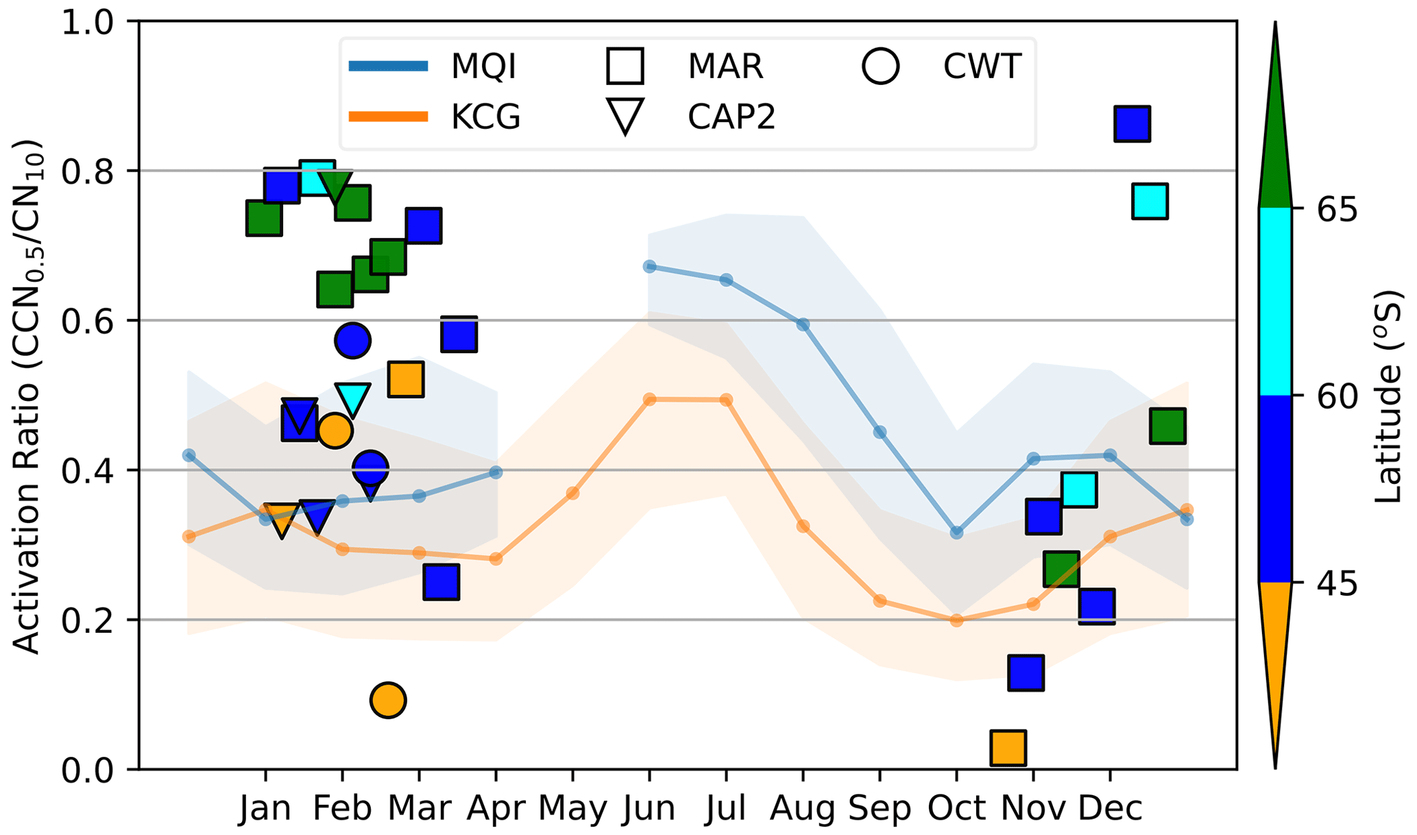
Figure 3Seasonal cycle of the activation ratio, CCN0.5 CN10, at both Macquarie Island and Kennaook / Cape Grim, with monthly medians (solid line) and interquartile range (shaded regions) shown. Overlaid on seasonal cycles are weekly medians from voyages where data are available, as in Fig. 2.
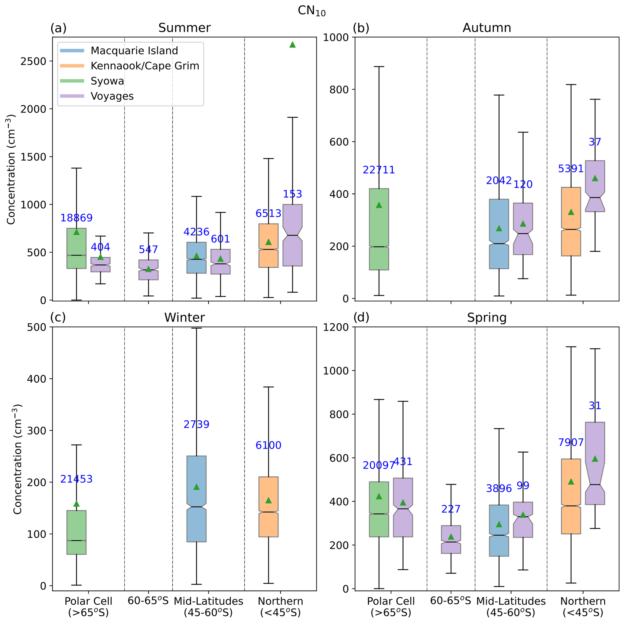
Figure 4Box plots of CN10 concentration categorised into seasons and latitudinal sectors in line with definitions by Humphries et al. (2021a). The 60–65∘ S sector is divided out as this is a boundary zone, the latitude of which varies significantly on daily timescales. All voyages are combined into a single data set (shown in purple). Box plots are standard Tukey plots with the boxes representing the 25th, 50th and 75th quartiles and the upper (lower) whisker being the first data points above (below) the 75th (25th) quartile plus (minus) 1.5 times the interquartile range. The notch in the box represents the confidence interval of the median, as calculated from 1000 bootstrap iterations. Green triangles represent the mean of each data set and the numbers above each box show the number of hourly observations used to calculate each box plot. A similar figure is shown in Fig. A6 with all y axis limits kept the same.
3.4 Latitudinal changes as a function of season
The data set being utilised in this study contains a valuable amount of both spatial and temporal information. In Figs. 4 and 5, population distributions are shown for CN10 and CCN0.5, respectively, split into seasons and previously described latitudinal bands (accompanying summary statistics are presented in Appendix Tables A1 and A2).
3.4.1 CN10
Summer CN10 data (Fig. 4a) confirm the latitudinal summertime patterns observed by Humphries et al. (2021a), where the highest concentrations are observed in the northern sector at latitudes lower than 45∘ S; the lowest concentrations are observed in the midlatitudes of the Southern Ocean (45 and 65∘ S), and a small increase in concentration is observed in the high-latitude bin (>65∘ S). Voyage and station data both agree well within each latitudinal band, except for the polar cell band. This is consistent with previous observations (Humphries et al., 2016, 2021a) which found that concentrations within the sea ice region around the Antarctic continent (termed the Antarctic Sea Ice Atmospheric Compositional Zone; ASIACZ) exhibited distinctly different aerosol properties to observations on the continent itself. We note that this is the first time continental and ASIACZ data sets have been obtained simultaneously for a direct comparison and suggests that the location of the ACFA during this period was somewhere between 65 and 69∘ S (69∘ S being the latitude of SYO).
There are no voyage data in autumn in the ACFA and ASIACZ latitudes (Fig. 4b). Voyage data agree well with station data at midlatitudes; however, this is not the case at the northern latitudes where voyage data are higher than station data from KCG. This is likely a result of the low sample size of voyage data in this sector and also of the fact that voyage data are not filtered for baseline conditions (i.e. wind directions and radon concentrations) like KCG data are, resulting in a higher continental influence. Again, the northerly bin shows the highest concentrations, which decrease further south. During this season, SYO data are comparable with midlatitude data, albeit with a slightly elevated upper 50 % of data, likely driven by the comparatively higher March concentrations reflecting the later summertime peak discussed early (Fig. 2b).
No voyage data exist during the winter months (Fig. 4c), meaning we only have station data to understand latitudinal differences, and only very limited information can be gained about the ASIACZ and ACFA region during this period. Results here reaffirm what was concluded from Fig. 2b where populations observed at KCG and MQI are similar, reflecting the dominance of sea salt aerosol and their similar proximity to the open ocean. The slightly higher concentrations observed at MQI is likely the result of it being closer to the sea surface, its inlet being only 10 m above sea level compared with 94 m at KCG. SYO's concentrations are substantially lower (medians approximately half of northern stations) resulting from the significant isolation of the station from the open ocean (∼1000 km) in winter.
We are fortunate to have a significant number of voyage data available during the spring months (Fig. 4d), a result of SIPEXII directly targeting the mid-spring season and MARCUS observations beginning in mid-October in line with when resupply operations for Australia's Antarctic programme become feasible. Springtime latitudinal patterns in general follow those of summer: northern concentrations are the highest and are followed by those at the highest latitudes, and the lowest concentrations are found in the midlatitudes. Unlike summertime concentrations where data from SYO and voyages in the polar cell were significantly different (medians of 468 and 368 cm−3, respectively), observations in springtime are almost identical (343 and 366 cm−3, respectively). It is worth noting here that while there is good agreement between springtime CN10 concentrations, previous analysis (Humphries et al., 2016) of SIPEXII data and comparison with the literature show that there are significant differences if CN3 concentrations are compared, suggesting a strong source of recently nucleated particles in the ASIACZ that is absent in coastal regions. It is suggested that observations of CN3 are an important enhancement to measurement programmes in this region in order to understand the drivers of this change (noting that this parameter is available for KCG and many of the voyages utilised in this study). The difference between concentrations observed in the polar cell and those in the 60–65∘ S latitudinal band is also striking, and would suggest that in springtime, this band is actually more reflective of midlatitude marine aerosol populations. Both of these features (i.e. the differences in the polar cell band between spring and summer and the springtime difference between the polar cell and the 60–65∘ S bin) together suggest that the location of the ACFA in springtime is much farther north than in summer. This is consistent with the understanding that the position of the ACFA is driven largely by meteorology and is a somewhat real-time realisation of the forces that create the atmospheric polar front (Humphries et al., 2016).
3.4.2 CCN
When looking at CCN0.5 spatial distributions (Fig. 5), we are unfortunately missing valuable data from SYO to give us insight into the differences between the ASIACZ and coastal Antarctica. Analyses of available data show that summertime CCN (Fig. 5a) are again consistent with spatial patterns derived from previous publications (Humphries et al., 2021a), with the highest concentrations observed in the northern sector, followed by the lowest concentration in the midlatitudes and a substantial increase in the polar cell bin south of 65∘ S. Concentrations in the 60–65∘ S sector fall within those expected at midlatitudes during the summer period. Interestingly, voyage data in the midlatitudes are higher than those observed at MQI or in the 60–65∘ S sector and are actually more in line with populations observed in the northern sector. This is the case for all voyages where data are available (MARCUS, CAPRICORN2, Cold Water Trial and PCAN); however, MARCUS is distinctly higher (not shown). Since this is not apparent in the CN10 data (Fig. 4a), it would suggest that a big difference in the latitudinal patterns that we observe is actually in the size distribution, where the northern sector has a strong and persistent Aitken mode that is significantly weaker in more southerly locations. Further analysis of aerosol size distributions, decomposed into finer-scale (e.g. 5∘) latitudinal bands, would help shed light on these changes. These data are available from the GAW capability of the RV Investigator station for many years and will be a topic of a future publication. It is worth noting here that voyage data in the northerly sector are significantly higher than those observed at KCG in summer. It is likely that this is a result of low sampling number and that voyage data in the sector are not filtered for continental influence using radon like they are at KCG.
Autumn voyage data (Fig. 5b) are consistent with the expected pattern; however, concentrations in the northerly sector are drastically higher than those observed at KCG. This is likely a result of the small sample size (only 77 h points) that is biased towards the early autumn months when many of these voyages were ending their summer campaigns. Given the significant changes that occur in autumn, the timing of the sampling has a big influence on the data. In addition, voyage data are not filtered for continental influence like KCG data are, meaning that voyage data in the northerly sector are likely to be influenced by Tasmanian outflow. Data from MQI are substantially higher than at KCG (a feature that is also observed in winter data in Fig. 5c) and are also higher than voyages in the midlatitude sector. This is driven by the unexplained late-autumn/winter peak in CCN observed at MQI previously discussed.
The limited voyage CCN0.5 data during springtime show significantly lower concentrations in the north compared to those south of 60∘ S. Although the number of hourly samples available from voyages during this time of year is limited, this change could be explained by the rapid increase in phytoplankton and sea ice algae that is concentrated more at higher latitudes than in the north. A word of caution is warranted here though: the low sample number could be significantly biasing the results, particularly given that springtime is known to be a period of significant change in the region, meaning that a small sample size at one particular period is not reflective of the entire season. This is likely the reason that voyage data do not compare well with station data during both springtime and autumn. This is a key point that reiterates the importance of long-term sampling rather than just relying on campaign observations, particularly in shoulder seasons.
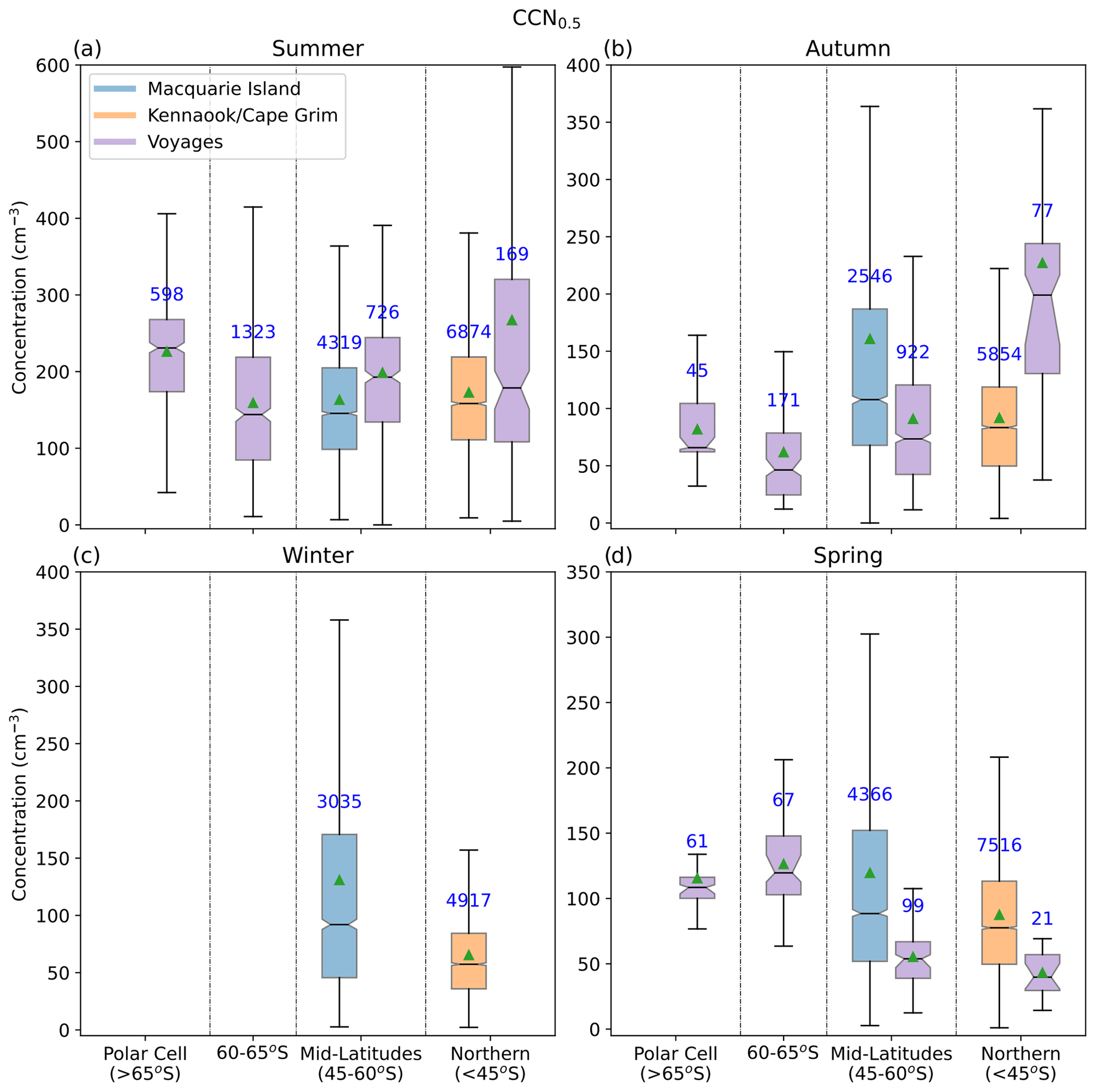
Figure 5As in previous figure but for CCN0.5. A similar figure is shown in Fig. A7 with all y axis limits kept the same.
While there are some important differences between voyage and station data which can be explained largely by sampling bias, it can be concluded from these data that, in general, long-term stations are good representations of their respective latitudinal bands. Although we are fortunate to have 2 years of recent data from MQI, the establishment of long-term observations at this location is imperative to monitor the changing climate in this sensitive region. The infrastructure for long-term observations already exists (e.g. Stavert et al., 2019), meaning that it is just the funding that is required. SYO's aerosol programme is invaluable and would be significantly enhanced by the addition of routine CCN and CN3 observations.
Long-term observations within the atmospherically distinct and spatially varying ASIACZ are an important missing part of the puzzle, resulting in a distinct absence or sparsity of data in shoulder and winter seasons. Long-term observations in this region would be logistically very challenging given the dynamic nature of the pack-ice environment. An ideal way to improve these observations is to establish long-term measurements programmes aboard ice-breaking vessels frequenting the Antarctic continent. This would establish frequent, repeated observations of the region and importantly a crossing of the ACFA (thereby improving the characterisation of its varying location). The primary limiting factor though is that observations outside of resupply seasons do not occur, resulting in no observations in winter and possibly autumn (depending on the vessel). Consideration of low-power, unattended buoys outfitted with suitable instrumentation for the observations of atmospheric composition may also be possible as technology improves. Logistically, long-term winter observations may be out of reach at this point in time; however, there is already discussion in the community about undertaking a year-long campaign in the Antarctic region, similar to the MOSAiC campaign (Shupe et al., 2020) undertaken in the Arctic in 2019–2020. Such a campaign would be a step change in Antarctic science across a range of disciplines that are limited by similar seasonal constraints.
Observations of CN10 and CCN from a 2-year campaign at Macquarie Island (MQI; 58.5∘ S, 158.9∘ E) between March 2016 and March 2018 are presented for the first time. Seasonal cycles show low concentrations typical of other sites in the region, with summer maxima and winter minima, driven primarily by biological emissions. Seasonal cycles were compared with two other long-term stations in the region: Kennaook / Cape Grim, Australia (KCG; 40.7∘ S, 144.7∘ E), and Syowa station, Antarctica (SYO; 69.0∘ S, 39.6∘ E).
The timing of the seasonal features in CN10 differs between each of the long-term stations. Summer maxima occurred in January at the Southern Ocean sites but were delayed by 1 month at SYO. Autumn decreases occur rapidly at SYO and MQI, with a more gradual decline at KCG. Winter minima lasted the longest at MQI (May through September), followed by SYO (May to August) and KCG, which had the shortest low (June to August). Aerosol populations at both KCG and SYO began increasing at the end of winter in August; however, concentrations at MQI only began ramping up strongly in November. Most of these features could be explained by the spatial and seasonal changes in phytoplankton communities across the region.
For CCN, data were unavailable from SYO, so a detailed latitudinal understanding could not be obtained. However, the differences at KCG between the CN and CCN are worth noting, with the former's summertime maximum enduring for much longer (10 months) than the latter's (7 months). At MQI, the summertime maximum of CCN0.5 is not as strong as that observed at KCG; however, a peculiar increase in CCN concentration across all supersaturations is observed in May and June 2016. Unfortunately, instrument failures at this time of year in the second year of observations prevented confirmation that this was a persistent feature or an anomaly occurring in just that year. This increase did not correlate with radon or any meteorological parameters.
Activation ratio data showed winter maxima reflective of the absence of secondary aerosols that drive this ratio down, with primarily only sea salt aerosol remaining. Activation ratios at MQI in this period were 0.2 higher than those at KCG, likely the result of the station being further away from biological sources still active in the winter. Summer observations in the high latitudes observed very high activation ratios of up to 0.8. Given the very high abundance of phytoplankton communities in this region, it is likely that precursor concentrations are strong enough to grow secondary aerosol populations to CCN active sizes. Given the outflow of air masses across the Southern Ocean from this region, this is an important source of CCN for the Southern Ocean region as a whole.
Analysis of how latitudinal gradients change with seasons shows that summertime CN and CCN data all show the highest concentrations in the northern sector, low concentrations in the mid-Southern Ocean latitudes and a modest increase in the polar sector. This pattern is also consistent for shoulder seasons; however, the winter pattern differs significantly, with consistent concentrations at both midlatitude and northern latitude sites and a significant decrease at SYO. A detailed latitudinal breakdown for seasons outside of summer was not possible because of the significant dearth of voyage data. The location of the ACFA was found to vary consistently with seasonal expectations, where springtime position is further north compared to springtime observations. Again, characterising its location in autumn and winter seasons is not possible because of the lack of ship data during these periods.
While this 2-year data set at Macquarie Island is an important step forward in our understanding of the seasonal cycle in this region, it was limited both in duration and the types of instrumentation. In addition to the establishment of new long-term monitoring stations at both mid-Southern Ocean latitudes, within the Antarctic sea ice region and on the Antarctic continent, these studies repeatedly highlight the requirement for enhancing all long-term station observations to include, at a minimum, CN3, CN10, CCN and aerosol size distributions. Instrumentation for these measurements is mature enough to be largely automated and run with only minimal on-the-ground technical support together with remote access. The addition of composition information is highly desired but is not as automated and can be more expensive.
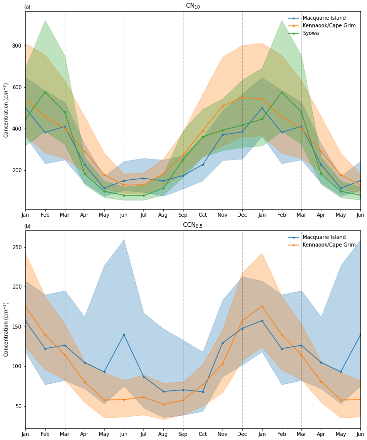
Figure A1Annual cycles of CN10 (a) and CCN0.5 (b) at Macquarie Island (blue), Kennaook / Cape Grim (orange) and Syowa (green). The first 6 months are repeated to show the seasonal cycle over 18 months to enable visibility of both summer maxima and winter minima.
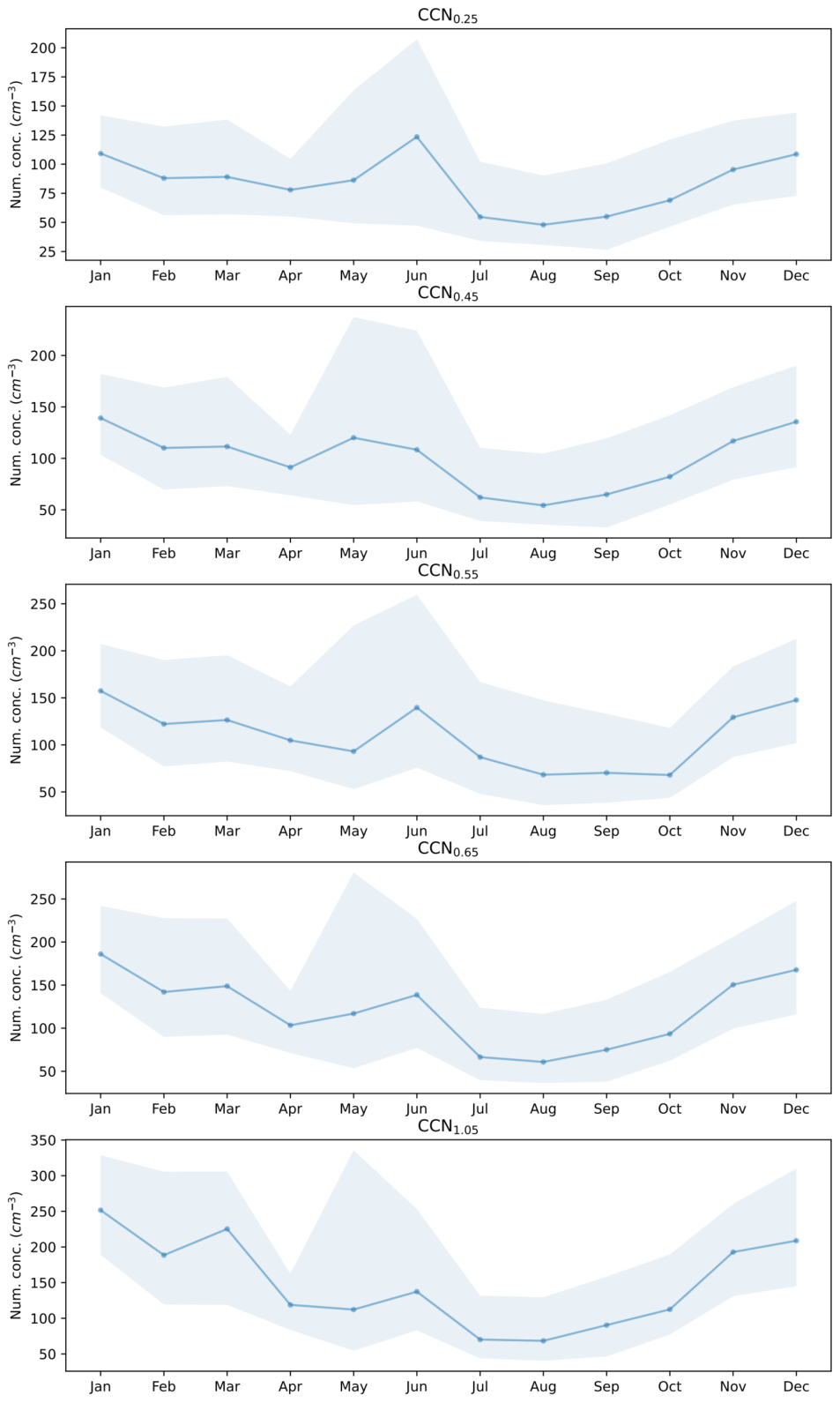
Figure A2Annual cycles of CCN0.5 at Macquarie Island for all five supersaturations measured.
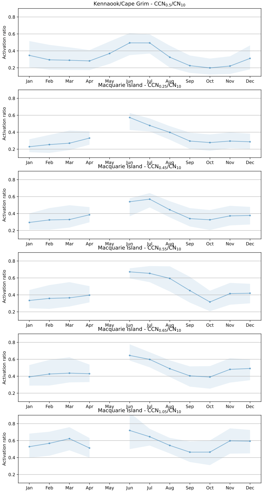
Figure A3Annual cycles of the CCN activation ratio for Kennaook / Cape Grim (top) and then all observed supersaturations at Macquarie Island. Unfortunately, instrument malfunctions of either the CPC or CCNC resulted in no ratio data available for May and the first half of June at Macquarie Island.
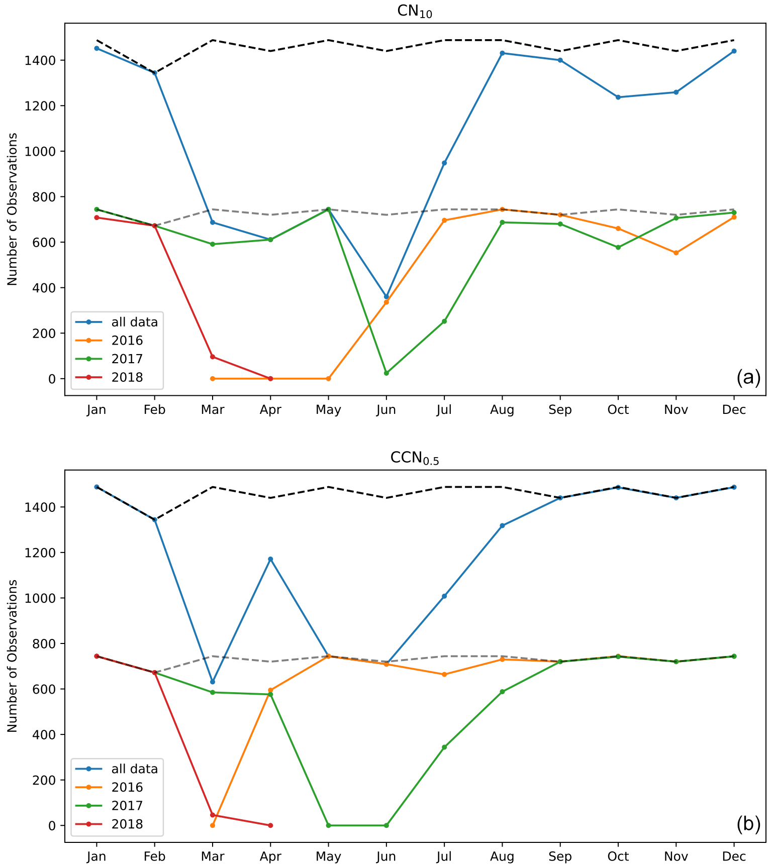
Figure A4Number of hourly data points available per month from Macquarie Island during the 2 years for both CN10 (a) and CCN0.5 (b). Data are shown for the full campaign and then separately for each year. The grey dashed line is a reference point for the maximum number of hours available in a particular month of each year, while the black dashed line is similar but for the maximum available during a particular month over the entirety of the campaign.
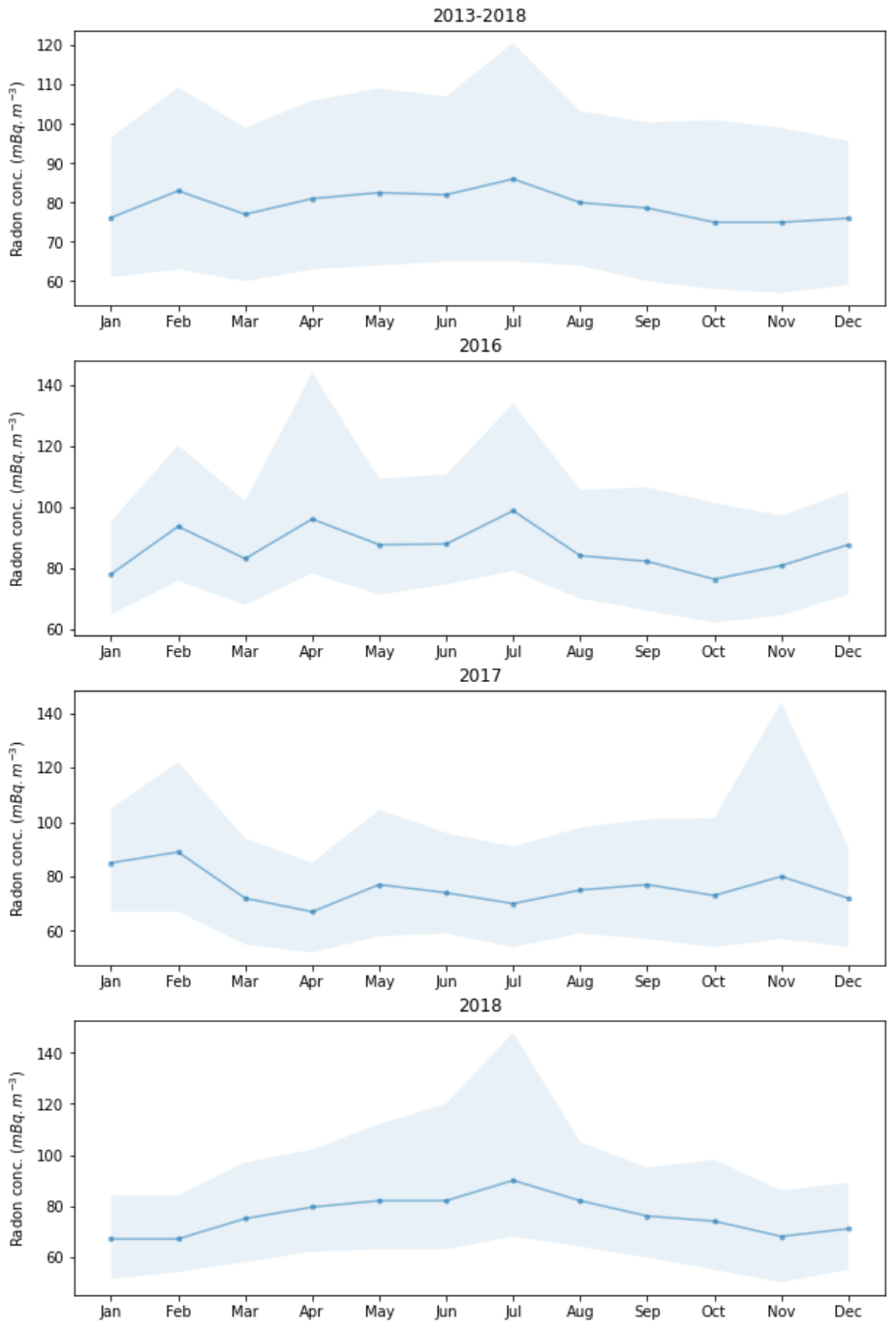
Figure A5Annual cycles of radon for the 6 years of data available (top) and each separate year of the ACRE campaign. Note that 2016 is where the CCN anomaly is observed.
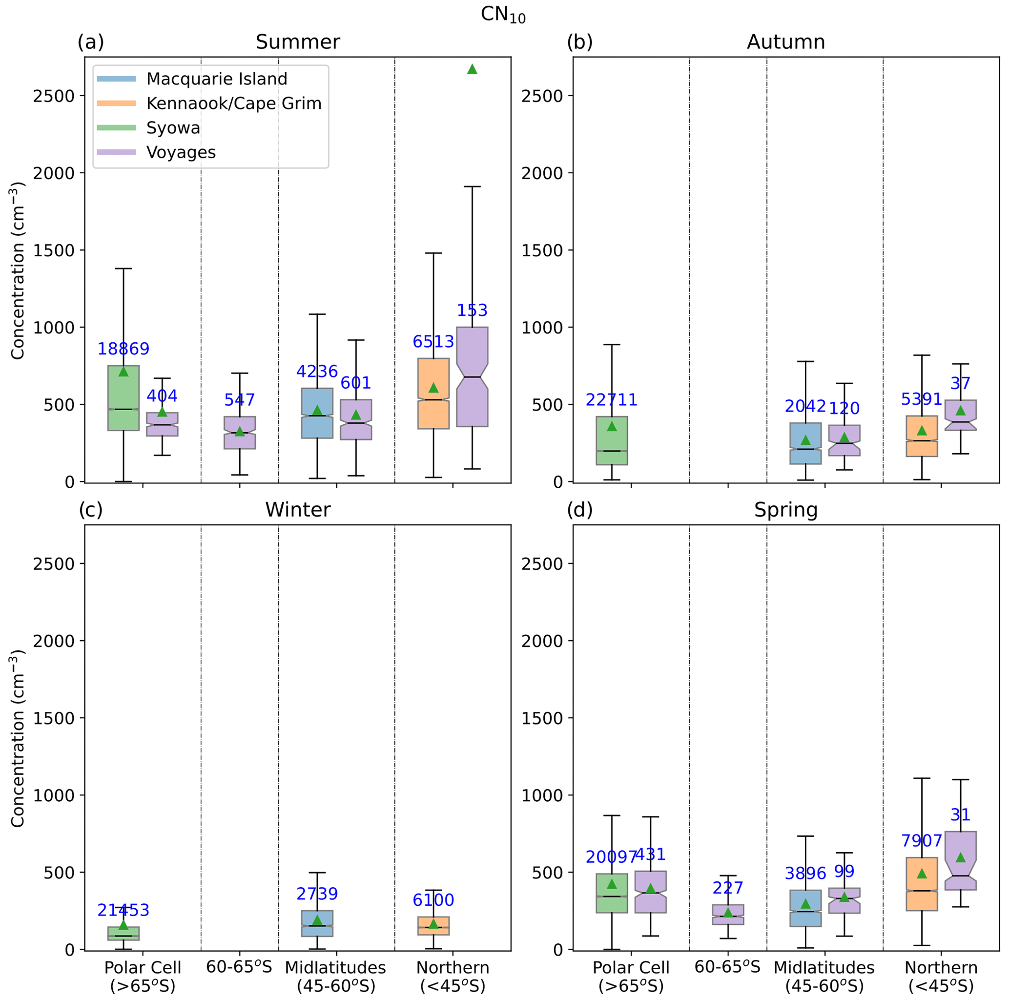
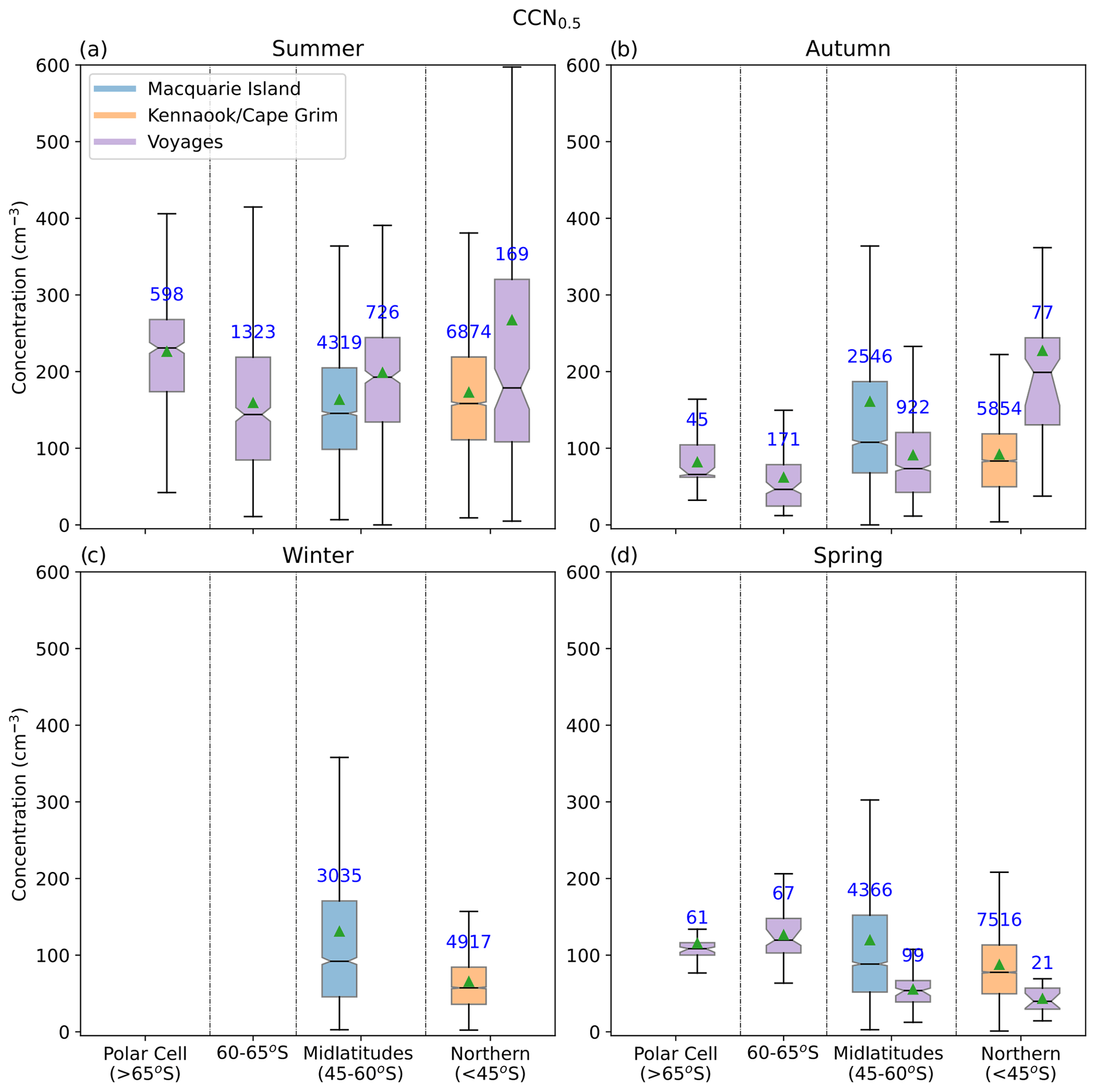
Table A1Seasonal summary statistics from stations and voyages for CN10.
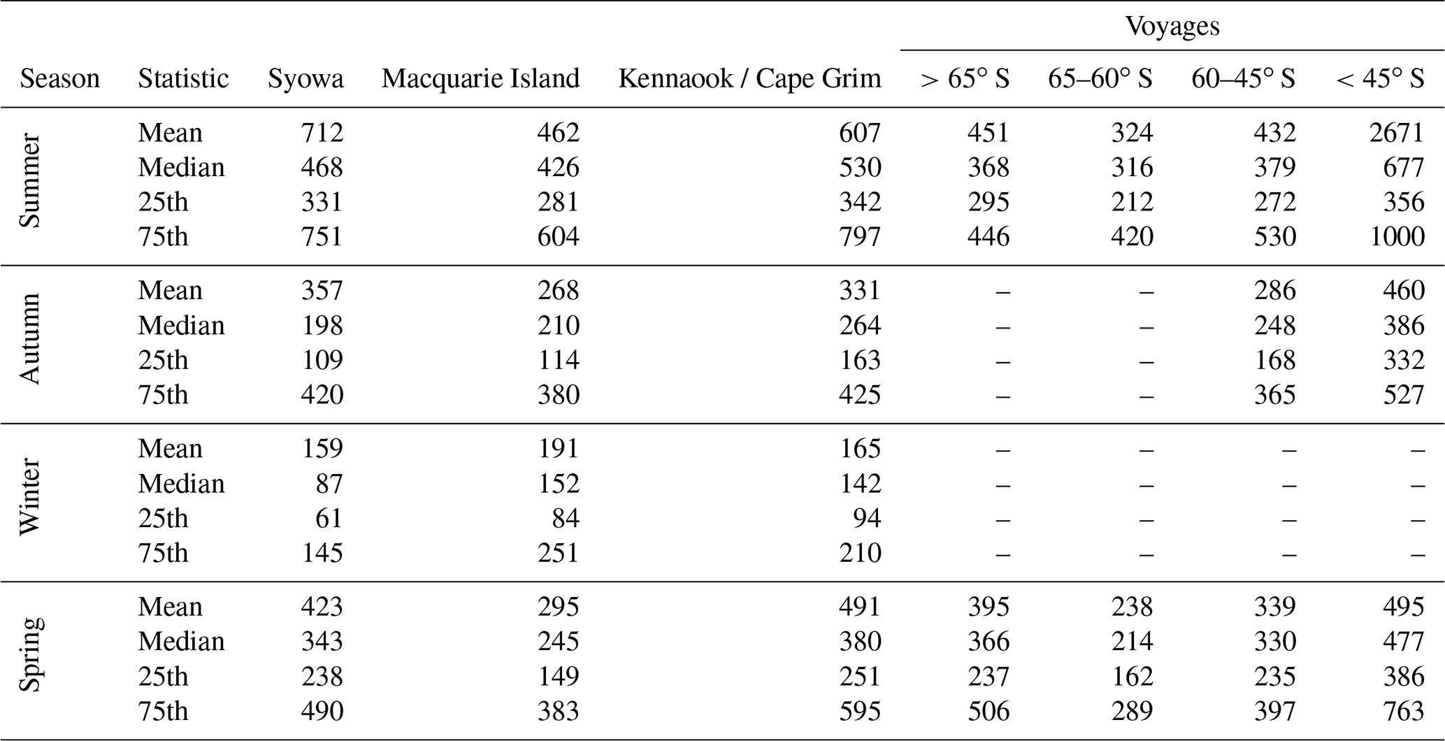
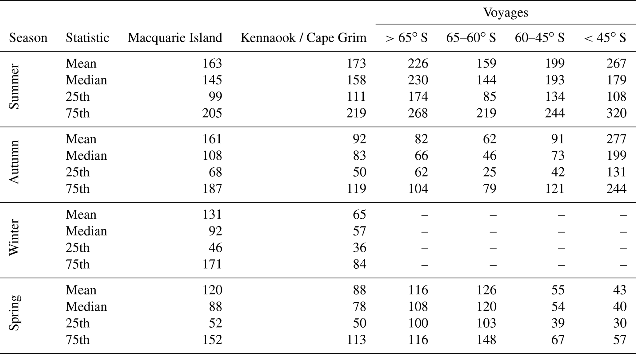
Table A2Seasonal summary statistics from stations and voyages for CCN0.5.
All data and samples are made publicly available in accordance with funder (see Acknowledgements) policies. CN and CCN data from Macquarie Island are available at https://doi.org/10.25919/g7jx-k629 (Humphries et al., 2021c). Data from Kennaook / Cape Grim are available at the World Data Centre for Aerosols at https://ebas-data.nilu.no (Keywood et al., 2023a, b). Syowa data are available at https://doi.org/10.17592/002.2023030399 (Hara, 2023). Data from MARCUS are available at https://doi.org/10.25919/ezp0-em87 (Humphries, 2020). Data from SIPEXII are available from https://doi.org/10.4225/15/5342423241BE4 (Humphries et al., 2014). Cold Water Trial data are available at https://doi.org/10.25919/ytsw-9610 (Humphries et al., 2022b). CAPRICORN1 data are available at https://doi.org/10.25919/5f688fcc97166 (Protat and Humphries, 2020). Ice2Equator data are available at https://doi.org/10.25919/g07r-b187 (Humphries et al., 2022a). PCAN data are available at https://doi.org/10.25919/xs0b-an24 (Humphries et al., 2020). CAPRICORN2 data are available at https://doi.org/10.25919/2h1c-t753 (Humphries et al., 2021b).
RSH wrote the paper and led the overall data analysis and interpretation. RSH undertook the aerosol study design, deployment, instrument maintenance and data handling for observations at Macquarie Island and during CAPRICORN1, CAPRICORN2, Ice2Equator, PCAN and SIPEX2. MDK is the lead scientist of the aerosol programme at Kennaook / Cape Grim and, together with JPW and JH, maintains the instruments, sampling infrastructure and data quality control. SPA and ARK were lead proponents of the ACRE, MICRE and MARCUS campaigns, and instrumental in their field deployment. KH is lead scientist of aerosol observations at Syowa Station. IMM, RSH, JPW and JH maintain the instrumentation and data production from aerosol instrumentation aboard the RV Investigator. AP was the chief scientist enabling observations during CAPRICORN1, CAPRICORN2 and Ice2Equator. JA, LTC, BM and ZDR maintained instrumentation and quality control of data for CAPRICORN1, CAPRICORN2, the Cold Water Trial and Ice2Equator. RS was chief scientist of the SIPEXII voyage and together with SRW was instrumental in ensuring high-quality measurements and in the data analysis. CJF and GRK were PIs of the MARCUS data. GGM was a chief scientist of CAPRICORN1 and CAPRICORN2 and was instrumental in undertaking analysis of these data as well as of MARCUS and ACRE data. GGM was chief scientist of the MARCUS campaign. SDC, AGW and ADG are the lead scientists of the radon programme at Macquarie Island.
The contact author has declared that none of the authors has any competing interests.
Publisher’s note: Copernicus Publications remains neutral with regard to jurisdictional claims in published maps and institutional affiliations.
Technical and logistical support for the deployment to Macquarie Island were provided by the Australian Antarctic Division, and we thank John French, Peter de Vries, Terry Egan, Nick Cartwright, Ken Barrett, George Brettingham-Moore and Emry William Crocker for their assistance.
MARCUS data were obtained from the Atmospheric Radiation Measurement (ARM) Program sponsored by the U.S. Department of Energy, Office of Science, Office of Biological and Environmental Research, and Climate and Environmental Sciences Division. We thank all the ARM technicians who collected the radiosonde and other data onboard RSV Aurora Australis. Technical, logistical and ship support for MARCUS was provided by the Australian Antarctic Division through Australia Antarctic Science projects 4292 and 4387, and we thank Steven Whiteside, Lloyd Symonds, Rick van den Enden, Peter de Vries, Chris Young and Chris Richards for assistance. The SIPEXII project was funded by the Australian Antarctic Science Grant Program (AAS Project 4032), and several RV Investigator voyages were supported by Australia Research Council Linkage Infrastructure, Equipment and Facilities grant LE150100048
The authors wish to thank the CSIRO Marine National Facility (MNF) for their support in the form of sea time on RV Investigator and associated support personnel, scientific equipment and data management. In particular we thank the Seagoing Instrumentation Team, the Data Acquisition and Processing Team, the Data Centre, and the MNF Operations Team for their technical, IT and logistical support.
The authors would also like to acknowledge the Australian Bureau of Meteorology for their long-term and continued support of the Kennaook / Cape Grim Baseline Air Pollution Monitoring Station and all the staff from the Bureau of Meteorology and CSIRO.
This research was supported in part by BER Award DESC0018995 (Gerald G. Mace and Ruhi S. Humphries) and NASA grants 80NSSC19K1251 (Gerald G. Mace). The work of Greg M. McFarquhar was funded by the United States Department of Energy Awards DE-SC0018626 and DE-SC0021159. Gourihar R. Kulkarni acknowledges support from the Office of Science of the U.S. Department of Energy (DOE) as part of the Atmospheric System Research Program. The work of Alain Protat was partly funded by the National Environmental Science Program (NESP), Australia.
This project received grant funding from the Australian Government as part of the Antarctic Science Collaboration Initiative programme (Ruhi S. Humphries, Melita D. Keywood, Alain Protat, Simon P. Alexander, Andrew R. Klekociuk).
This research was supported by the Australian Government (Australian Antarctic Science projects 4292, 4431, 4387 and 4032; Australian Research Council Linkage Infrastructure, Equipment and Facilities grant LE150100048; the National Environmental Science Program; the Antarctic Science Collaboration Initiative programme; ongoing support of Kennaook / Cape Grim through the Bureau of Meteorology; RV Investigator access via the Marine National Facility), the U.S. Department of Energy (grants DE-SC0018626, DESC0018995 and DE-SC0021159 and the Atmospheric System Research Program), and the National Aeronautics and Space Administration (grant no. 80NSSC19K1251).
This paper was edited by Jerome Brioude and reviewed by two anonymous referees.
Alexander, S. P. and Klekociuk, A. R.: Constraining Ice Water Content of Thin Antarctic Cirrus Clouds Using Ground-Based Lidar and Satellite Data, J. Atmos. Sci., 78, 1791–1806, https://doi.org/10.1175/JAS-D-20-0251.1, 2021. a
Alroe, J.: Emission Sources, Cloud-Relevant Properties and Variability of Aerosol over the Southern and Pacific Oceans, PhD thesis, Queensland University of Technology, https://doi.org/10.5204/thesis.eprints.209152, 2021. a
Alroe, J., Cravigan, L. T., Miljevic, B., Johnson, G. R., Selleck, P., Humphries, R. S., Keywood, M. D., Chambers, S. D., Williams, A. G., and Ristovski, Z. D.: Marine productivity and synoptic meteorology drive summer-time variability in Southern Ocean aerosols, Atmos. Chem. Phys., 20, 8047–8062, https://doi.org/10.5194/acp-20-8047-2020, 2020. a, b, c, d, e
Asmi, E., Frey, A., Virkkula, A., Ehn, M., Manninen, H. E., Timonen, H., Tolonen-Kivimäki, O., Aurela, M., Hillamo, R., and Kulmala, M.: Hygroscopicity and chemical composition of Antarctic sub-micrometre aerosol particles and observations of new particle formation, Atmos. Chem. Phys., 10, 4253–4271, https://doi.org/10.5194/acp-10-4253-2010, 2010. a
Ayers, G. P. and Gras, J. L.: Seasonal Relationship between Cloud Condensation Nuclei and Aerosol Methanesulphonate in Marine Air, Nature, 353, 834–835, https://doi.org/10.1038/353834a0, 1991. a
Bates, T. S., Huebert, B. J., Gras, J. L., Griffiths, F. B., and Durkee, P. A.: International Global Atmospheric Chemistry (IGAC) Project's First Aerosol Characterization Experiment (ACE 1): Overview, J. Geophys. Res., 103, 16297–16297, https://doi.org/10.1029/97JD03741, 1998. a, b
Bigg, E. K.: Long-Term Trends in Ice Nucleus Concentrations, Atmos. Res., 25, 409–415, https://doi.org/10.1016/0169-8095(90)90025-8, 1990a. a
Bigg, E. K.: Aerosol over the Southern Ocean, Atmos. Res., 25, 583–600, https://doi.org/10.1016/0169-8095(90)90039-F, 1990b. a
Bigg, E. K., Gras, J. L., and Evans, C.: Origin of Aitken Particles in Remote Regions of the Southern Hemisphere, J. Atmos. Chem., 1, 203–214, 1983. a, b
Bigg, E. K., Gras, J. L., and Evans, C.: Origin of Aitken Particles in Remote Regions of the Southern Hemisphere, J. Atmos. Chem., 1, 203–214, https://doi.org/10.1007/BF00053841, 1984. a, b
Boers, R.: Influence of Seasonal Variation in Cloud Condensation Nuclei, Drizzle, and Solar Radiation, on Marine Stratocumulus Optical Depth, Tellus, 47B, 578–586, https://doi.org/10.3402/tellusb.v47i5.16073, 1995. a
Brechtel, F. J., Kreidenweis, S. M., and Swan, H. B.: Air Mass Characteristics, Aerosol Particle Number Concentrations, and Number Size Distributions at Macquarie Island during the First Aerosol Characterization Experiment (ACE 1), J. Geophys. Res.-Atmos., 103, 16351–16367, https://doi.org/10.1029/97jd03014, 1998. a, b
Brock, C. A., Williamson, C., Kupc, A., Froyd, K. D., Erdesz, F., Wagner, N., Richardson, M., Schwarz, J. P., Gao, R.-S., Katich, J. M., Campuzano-Jost, P., Nault, B. A., Schroder, J. C., Jimenez, J. L., Weinzierl, B., Dollner, M., Bui, T., and Murphy, D. M.: Aerosol size distributions during the Atmospheric Tomography Mission (ATom): methods, uncertainties, and data products, Atmos. Meas. Tech., 12, 3081–3099, https://doi.org/10.5194/amt-12-3081-2019, 2019. a
Carslaw, K. S., Lee, L. A., Reddington, C. L., Pringle, K. J., Rap, A., Forster, P. M., Mann, G. W., Spracklen, D. V., Woodhouse, M. T., Regayre, L. A., and Pierce, J. R.: Large Contribution of Natural Aerosols to Uncertainty in Indirect Forcing, Nature, 503, 67–71, https://doi.org/10.1038/nature12674, 2013. a
Chambers, S. D., Preunkert, S., Weller, R., Hong, S.-B., Humphries, R. S., Tositti, L., Angot, H., Legrand, M., Williams, A. G., Griffiths, A. D., Crawford, J., Simmons, J., Choi, T. J., Krummel, P. B., Molloy, S., Loh, Z., Galbally, I., Wilson, S., Magand, O., Sprovieri, F., Pirrone, N., and Dommergue, A.: Characterizing Atmospheric Transport Pathways to Antarctica and the Remote Southern Ocean Using Radon-222, Front. Earth Sci., 6, 190, https://doi.org/10.3389/feart.2018.00190, 2018. a
Choi, J., Son, S.-W., Lu, J., and Min, S.-K.: Further Observational Evidence of Hadley Cell Widening in the Southern Hemisphere, Geophys. Res. Lett., 41, 2590–2597, https://doi.org/10.1002/2014GL059426, 2014. a
Claeys, M., Wang, W., Vermeylen, R., Kourtchev, I., Chi, X., Farhat, Y., Surratt, J. D., Gómez-González, Y., Sciare, J., and Maenhaut, W.: Chemical Characterisation of Marine Aerosol at Amsterdam Island during the Austral Summer of 2006–2007, J. Aerosol Sci., 41, 13–22, https://doi.org/10.1016/j.jaerosci.2009.08.003, 2010. a
Covert, D. S., Gras, J. L., Wiedensohler, A., and Stratmann, F.: Comparison of Directly Measured CCN with CCN Modeled from the Number-Size Distribution in the Marine Boundary Layer during ACE 1 at Cape Grim, Tasmania, J. Geophys. Res.-Atmos., 103, 16597–16608, https://doi.org/10.1029/98JD01093, 1998. a
Dall'Osto, M., Ovadnevaite, J., Paglione, M., Beddows, D. C. S., Ceburnis, D., Cree, C., Cortés, P., Zamanillo, M., Nunes, S. O., Pérez, G. L., Ortega-Retuerta, E., Emelianov, M., Vaqué, D., Marrasé, C., Estrada, M., Sala, M. M., Vidal, M., Fitzsimons, M. F., Beale, R., Airs, R., Rinaldi, M., Decesari, S., Cristina Facchini, M., Harrison, R. M., O'Dowd, C., and Simó, R.: Antarctic Sea Ice Region as a Source of Biogenic Organic Nitrogen in Aerosols, Sci. Rep., 7, 6047–6047, https://doi.org/10.1038/s41598-017-06188-x, 2017. a
Davis, S. M. and Rosenlof, K. H.: A Multidiagnostic Intercomparison of Tropical-Width Time Series Using Reanalyses and Satellite Observations, J. Climate, 25, 1061–1078, https://doi.org/10.1175/JCLI-D-11-00127.1, 2012. a
Deppeler, S. L. and Davidson, A. T.: Southern Ocean Phytoplankton in a Changing Climate, Front. Mar. Sci., 4, 40, https://doi.org/10.3389/fmars.2017.00040, 2017. a, b, c
Fossum, K. N., Ovadnevaite, J., Ceburnis, D., Dall'Osto, M., Marullo, S., Bellacicco, M., Simó, R., Liu, D., Flynn, M., Zuend, A., and O'Dowd, C.: Summertime Primary and Secondary Contributions to Southern Ocean Cloud Condensation Nuclei, Sci. Rep.-UK, 8, 13844, https://doi.org/10.1038/s41598-018-32047-4, 2018. a, b
Frey, W. R. and Kay, J. E.: The Influence of Extratropical Cloud Phase and Amount Feedbacks on Climate Sensitivity, Clim. Dynam., 50, 3097–3116, https://doi.org/10.1007/s00382-017-3796-5, 2018. a
Frossard, A. A., Russell, L. M., Burrows, S. M., Elliott, S. M., Bates, T. S., and Quinn, P. K.: Sources and Composition of Submicron Organic Mass in Marine Aerosol Particles, J. Geophys. Res.-Atmos., 119, 12977–13003, https://doi.org/10.1002/2014JD021913, 2014. a
Gettelman, A., Lin, L., Medeiros, B., and Olson, J.: Climate Feedback Variance and the Interaction of Aerosol Forcing and Feedbacks, J. Climate, 29, 6659–6675, https://doi.org/10.1175/JCLI-D-16-0151.1, 2016. a
Gras, J. L.: Ammonia and Ammonium Concentrations in the Antarctic Atmosphere, Atmos. Environ., 17, 815–818, 1983. a
Gras, J. L.: Cloud Condensation Nuclei over the Southern Ocean, Geophys. Res. Lett., 17, 1565–1567, https://doi.org/10.1029/GL017i010p01565, 1990. a
Gras, J. L.: Condensation Nucleus Size Distribution at Mawson, Antarctica: Seasonal Cycle, Atmos. Environ. A-Gen., 27, 1417–1425, https://doi.org/10.1016/0960-1686(93)90127-K, 1993. a, b
Gras, J. L. and Keywood, M.: Cloud condensation nuclei over the Southern Ocean: wind dependence and seasonal cycles, Atmos. Chem. Phys., 17, 4419–4432, https://doi.org/10.5194/acp-17-4419-2017, 2017. a, b, c, d, e
Hansen, G., Aspmo, K., Berg, T., Edvardsen, K., Fiebig, M., Kallenborn, R., Krognes, T., Lunder, C., Stebel, K., Schmidbauer, N., Solberg, S., and Yttri, K. E.: Atmospheric Monitoring at the Norwegian Antarctic Station Troll: Measurement Programme and First Results, Polar Res., 28, 353–363, https://doi.org/10.3402/polar.v28i3.6142, 2009. a
Hara, K.: Antarctic aerosol CN, National Institute of Polar Research [data set], https://doi.org/10.17592/002.2023030399, 2023. a, b
Hara, K., Osada, K., Nishita-Hara, C., Yabuki, M., Hayashi, M., Yamanouchi, T., Wada, M., and Shiobara, M.: Seasonal features of ultrafine particle volatility in the coastal Antarctic troposphere, Atmos. Chem. Phys., 11, 9803–9812, https://doi.org/10.5194/acp-11-9803-2011, 2011a. a
Hara, K., Osada, K., Nishita-Hara, C., and Yamanouchi, T.: Seasonal variations and vertical features of aerosol particles in the Antarctic troposphere, Atmos. Chem. Phys., 11, 5471–5484, https://doi.org/10.5194/acp-11-5471-2011, 2011b. a, b, c
Herenz, P., Wex, H., Mangold, A., Laffineur, Q., Gorodetskaya, I. V., Fleming, Z. L., Panagi, M., and Stratmann, F.: CCN measurements at the Princess Elisabeth Antarctica research station during three austral summers, Atmos. Chem. Phys., 19, 275–294, https://doi.org/10.5194/acp-19-275-2019, 2019. a
Hong, S.-b., Yoon, Y. J., Becagli, S., Gim, Y., Chambers, S., Park, K.-T., Park, S.-J., Traversi, R., Severi, M., Vitale, V., Kim, J.-H., Jang, E., Crawford, J., and Griffiths, A.: Seasonality of Aerosol Chemical Composition at King Sejong Station (Antarctic Peninsula) in 2013, Atmos. Environ., 223, 117185, https://doi.org/10.1016/j.atmosenv.2019.117185, 2020. a
Humphries, R. S.: MARCUS ARM CN and CCN Data Reprocessed to Remove Ship Exhaust Influence, CSIRO Data Access Portal [data set], https://doi.org/10.25919/ezp0-em87, 2020. a, b, c
Humphries, R. S., Wilson, S. R., Keywood, M. D., Ward, J., and Schofield, R.: In-Situ Total Aerosol Number Using Condensation Particle Counters as Observed during the SIPEX II Voyage of the Aurora Australis, 2012, 5. Australian Antarctic Data Centre [data set], https://doi.org/10.4225/15/5342423241BE4, 2014. a, b
Humphries, R. S., Schofield, R., Keywood, M. D., Ward, J., Pierce, J. R., Gionfriddo, C. M., Tate, M. T., Krabbenhoft, D. P., Galbally, I. E., Molloy, S. B., Klekociuk, A. R., Johnston, P. V., Kreher, K., Thomas, A. J., Robinson, A. D., Harris, N. R. P., Johnson, R., and Wilson, S. R.: Boundary layer new particle formation over East Antarctic sea ice – possible Hg-driven nucleation?, Atmos. Chem. Phys., 15, 13339–13364, https://doi.org/10.5194/acp-15-13339-2015, 2015. a, b
Humphries, R. S., Klekociuk, A. R., Schofield, R., Keywood, M., Ward, J., and Wilson, S. R.: Unexpectedly high ultrafine aerosol concentrations above East Antarctic sea ice, Atmos. Chem. Phys., 16, 2185–2206, https://doi.org/10.5194/acp-16-2185-2016, 2016. a, b, c, d, e, f, g
Humphries, R. S., McRobert, I. M., Ponsonby, W. A., Ward, J. P., Keywood, M. D., Loh, Z. M., Krummel, P. B., and Harnwell, J.: Identification of platform exhaust on the RV Investigator, Atmos. Meas. Tech., 12, 3019–3038, https://doi.org/10.5194/amt-12-3019-2019, 2019. a
Humphries, R. S., Simmons, J. B., McRobert, I. M., Ward, J., Keywood, M. D., Chambers, S. D., Griffiths, A. D., Williams, A. G., and Wilson, S. R.: Polar Cell Aerosol Nucleation – Atmospheric Measurements from the RV Investigator Voyage IN2017_V01, CSIRO Data Access Portal [data set], https://doi.org/10.25919/xs0b-an24, 2020. a, b
Humphries, R. S., Keywood, M. D., Gribben, S., McRobert, I. M., Ward, J. P., Selleck, P., Taylor, S., Harnwell, J., Flynn, C., Kulkarni, G. R., Mace, G. G., Protat, A., Alexander, S. P., and McFarquhar, G.: Southern Ocean latitudinal gradients of cloud condensation nuclei, Atmos. Chem. Phys., 21, 12757–12782, https://doi.org/10.5194/acp-21-12757-2021, 2021. a, b, c, d, e, f, g, h, i, j, k, l
Humphries, R. S., McRobert, I. M., Ward, J., Harnwell, J., and Keywood, M. D.: CAPRICORN2 – Atmospheric Aerosol Measurements from the RV Investigator Voyage IN2018_V01, CSIRO Data Access Portal [data set], https://doi.org/10.25919/2h1c-t753, 2021b. a, b
Humphries, R. S., Ward, J., Keywood, M. D., and Alexander, S. P.: Atmospheric Aerosol and Cloud Condensation Nuclei Concentrations from Macquarie Island from 2016 to 2018, CSIRO Data Access Portal [data set], https://doi.org/10.25919/g7jx-k629, 2021c. a, b
Humphries, R. S., Ward, J., McRobert, I., Thomas, S., Harnwell, J., Marouchos, A., Keywood, M., Molloy, S. B., Loh, Z. M., Krummel, P. B., Ponsonby, W., and Crawford, H.: _RV Investigator – the World's First Mobile GAW Station, in prep., 2021d.
Humphries, R. S., Alroe, J., Ristovski, Z. D., Keywood, M. D., Ward, J. D., McRobert, I. M., Cravigan, L. T., and Brown, R.: Aerosol Properties, Ice-edge to Equator Voyage (IN2016_V03): CN3 and CCN, CSIRO Data Access Portal [data set], https://doi.org/10.25919/g07r-b187, 2022a. a, b
Humphries, R. S., Alroe, J., Ward, J. D., Keywood, M. D., McRobert, I. M., Cravigan, L. T., and Ristovski, Z. D.: Aerosol Properties, Cold Water Trial Voyage (IN2015_E01): CN3 and CCN, CSIRO Data Access Portal [data set], https://doi.org/10.25919/ytsw-9610, 2022b. a, b
IPCC: Clouds and Aerosols, in: Climate Change 2013 – The Physical Science Basis: Working Group I Contribution to the Fifth Assessment Report of the Intergovernmental Panel on Climate Change, Cambridge University Press, Cambridge, 571–658, https://doi.org/10.1017/CBO9781107415324.016, 2014. a, b
IPCC: The Earth's Energy Budget, Climate Feedbacks, and Climate Sensitivity, in: Climate Change 2021: The Physical Science Basis. Contribution of Working Group I to the Sixth Assessment Report of the Intergovernmental Panel on Climate Change, Cambridge University Press, Cambridge, 923–1054, https://doi.org/10.1017/9781009157896.009, 2021. a
Jang, E., Park, K.-T., Yoon, Y. J., Kim, K., Gim, Y., Chung, H. Y., Lee, K., Choi, J., Park, J., Park, S.-J., Koo, J.-H., Fernandez, R. P., and Saiz-Lopez, A.: First-Year Sea Ice Leads to an Increase in Dimethyl Sulfide-Induced Particle Formation in the Antarctic Peninsula, Sci. Total Environ., 803, 150002, https://doi.org/10.1016/j.scitotenv.2021.150002, 2022. a, b
Jimi, S. I., Gras, J., Siems, S. T., and Krummel, P. B.: A Short Climatology of Nanoparticles at the Cape Grim Baseline Air Pollution Station, Tasmania, Environ. Chem., 4, 301–309, https://doi.org/10.1071/EN07038, 2007. a
Keywood, M. D., Ward, J., and Derek, N.: Cloud Condensation Nuclei Number Concentration, World Data Centre for Aerosols, https://ebas-data.nilu.no, last access: 16 March 2023a. a
Keywood, M. D., Ward, J., and Derek, N.: Particle Number Concentration, World Data Centre for Aerosols, https://ebas-data.nilu.no, last access: 16 March 2023b. a
Kim, M. J., Novak, G. A., Zoerb, M. C., Yang, M., Blomquist, B. W., Huebert, B. J., Cappa, C. D., and Bertram, T. H.: Air-Sea Exchange of Biogenic Volatile Organic Compounds and the Impact on Aerosol Particle Size Distributions, Geophys. Res. Lett., 44, 3887–3896, https://doi.org/10.1002/2017GL072975, 2017. a
Koponen, I. K., Virkkula, A., Hillamo, R., Kerminen, V.-M., and Kulmala, M.: Number Size Distributions and Concentrations of the Continental Summer Aerosols in Queen Maud Land, Antarctica, J. Geophys. Res.-Atmos., 108, 4587–4587, https://doi.org/10.1029/2003jd003614, 2003. a
Kreidenweis, S. M., McInnes, L. M., and Brechtel, F. J.: Observations of Aerosol Volatility and Elemental Composition at Macquarie Island during the First Aerosol Characterization Experiment (ACE 1), J. Geophys. Res.-Atmos., 103, 16511–16524, https://doi.org/10.1029/98JD00800, 1998. a, b
Kremser, S., Harvey, M., Kuma, P., Hartery, S., Saint-Macary, A., McGregor, J., Schuddeboom, A., von Hobe, M., Lennartz, S. T., Geddes, A., Querel, R., McDonald, A., Peltola, M., Sellegri, K., Silber, I., Law, C. S., Flynn, C. J., Marriner, A., Hill, T. C. J., DeMott, P. J., Hume, C. C., Plank, G., Graham, G., and Parsons, S.: Southern Ocean cloud and aerosol data: a compilation of measurements from the 2018 Southern Ocean Ross Sea Marine Ecosystems and Environment voyage, Earth Syst. Sci. Data, 13, 3115–3153, https://doi.org/10.5194/essd-13-3115-2021, 2021. a
Kuang, C., Salwen, C., Boyer, M., and Singh, A.: Atmospheric Radiation Measurement (ARM) User Facility, 2017, Updated Hourly, Condensation Particle Counter (AOSCPCF), 2017-10-29 to 2018-03-26, ARM Mobile Facility (MAR) Hobart, AUS to Antarctic Coast – Resupply Ship Aurora Australis, AMF2 (M1), 2018.
Kubicki, M., Odzimek, A., and Neska, M.: Relationship of Ground-Level Aerosol Concentration and Atmospheric Electric Field at Three Observation Sites in the Arctic, Antarctic and Europe, Atmos. Res., 178–179, 329–346, https://doi.org/10.1016/j.atmosres.2016.03.029, 2016. a
Kulkarni, G. R., Flynn, C., and Koontz, A.: Atmospheric Radiation Measurement (ARM) User Facility, 2017, Updated Hourly, Cloud Condensation Nuclei Particle Counter (AOSCCN100), 2017-10-29 to 2018-03-24, ARM Mobile Facility (MAR) Hobart, AUS to Antarctic Coast – Resupply Ship Aurora Australis, AMF2 (M1)., 2018.
Kyrö, E.-M., Kerminen, V.-M., Virkkula, A., Dal Maso, M., Parshintsev, J., Ruíz-Jimenez, J., Forsström, L., Manninen, H. E., Riekkola, M.-L., Heinonen, P., and Kulmala, M.: Antarctic new particle formation from continental biogenic precursors, Atmos. Chem. Phys., 13, 3527–3546, https://doi.org/10.5194/acp-13-3527-2013, 2013. a
Lana, A., Bell, T. G., Simó, R., Vallina, S. M., Ballabrera-Poy, J., Kettle, A. J., Dachs, J., Bopp, L., Saltzman, E. S., Stefels, J., Johnson, J. E., and Liss, P. S.: An Updated Climatology of Surface Dimethlysulfide Concentrations and Emission Fluxes in the Global Ocean, Global Biogeochem. Cy., 25, GB1004, https://doi.org/10.1029/2010gb003850, 2011. a
Law, C. S., Smith, M. J., Harvey, M. J., Bell, T. G., Cravigan, L. T., Elliott, F. C., Lawson, S. J., Lizotte, M., Marriner, A., McGregor, J., Ristovski, Z., Safi, K. A., Saltzman, E. S., Vaattovaara, P., and Walker, C. F.: Overview and preliminary results of the Surface Ocean Aerosol Production (SOAP) campaign, Atmos. Chem. Phys., 17, 13645–13667, https://doi.org/10.5194/acp-17-13645-2017, 2017. a
Li, J., Michalski, G., Davy, P., Harvey, M., Katzman, T., and Wilkins, B.: Investigating Source Contributions of Size-Aggregated Aerosols Collected in Southern Ocean and Baring Head, New Zealand Using Sulfur Isotopes, Geophys. Res. Lett., 45, 3717–3727, https://doi.org/10.1002/2018GL077353, 2018. a
Lucas, C., Timbal, B., and Nguyen, H.: The Expanding Tropics: A Critical Assessment of the Observational and Modeling Studies, Wiley Interdisciplinary Reviews: Climate Change, 5, 89–112, https://doi.org/10.1002/wcc.251, 2014. a
Mace, G. G. and Protat, A.: Clouds over the Southern Ocean as Observed from the R/V Investigator during CAPRICORN. Part I: Cloud Occurrence and Phase Partitioning, J. Appl. Meteorol. Clim., 57, 1783–1803, https://doi.org/10.1175/JAMC-D-17-0194.1, 2018. a, b
Mace, G. G., Protat, A., Humphries, R. S., Alexander, S. P., McRobert, I. M., Ward, J., Selleck, P., Keywood, M., and McFarquhar, G. M.: Southern Ocean Cloud Properties Derived From CAPRICORN and MARCUS Data, J. Geophys. Res.-Atmos., 126, e2020JD033368, https://doi.org/10.1029/2020JD033368, 2021. a
Marchand, R., Wood, R., Bretherton, C., McFarquhar, G., Protat, A., Quinn, P., Siems, S., Jakob, C., Alexander, S., and Weller, B.: Southern Ocean Clouds, Radiation, Aerosol Transport Experimental Study – White Paper, 2014. a
McCoy, I. L., McCoy, D. T., Wood, R., Regayre, L., Watson-Parris, D., Grosvenor, D. P., Mulcahy, J. P., Hu, Y., Bender, F. A.-M., Field, P. R., Carslaw, K. S., and Gordon, H.: The Hemispheric Contrast in Cloud Microphysical Properties Constrains Aerosol Forcing, P. Natl. Acad. Sci. USA, 117, 18998–19006, https://doi.org/10.1073/pnas.1922502117, 2020. a
McFarquhar, G. M., Bretherton, C. S., Marchand, R., Protat, A., DeMott, P. J., Alexander, S. P., Roberts, G. C., Twohy, C. H., Toohey, D., Siems, S., Huang, Y., Wood, R., Rauber, R. M., Lasher-Trapp, S., Jensen, J., Stith, J. L., Mace, J., Um, J., Järvinen, E., Schnaiter, M., Gettelman, A., Sanchez, K. J., McCluskey, C. S., Russell, L. M., McCoy, I. L., Atlas, R. L., Bardeen, C. G., Moore, K. A., Hill, T. C. J., Humphries, R. S., Keywood, M. D., Ristovski, Z., Cravigan, L., Schofield, R., Fairall, C., Mallet, M. D., Kreidenweis, S. M., Rainwater, B., D'Alessandro, J., Wang, Y., Wu, W., Saliba, G., Levin, E. J. T., Ding, S., Lang, F., Truong, S. C. H., Wolff, C., Haggerty, J., Harvey, M. J., Klekociuk, A. R., and McDonald, A.: Observations of Clouds, Aerosols, Precipitation, and Surface Radiation over the Southern Ocean: An Overview of CAPRICORN, MARCUS, MICRE, and SOCRATES, B. Am. Meteorol. Soc., 102, E894–E928, https://doi.org/10.1175/BAMS-D-20-0132.1, 2021. a, b, c
O'Dowd, C. D., Lowe, J. A., Smith, M. H., Davison, B., Hewitt, C. N., and Harrison, R. M.: Biogenic Sulphur Emissions and Inferred Non-Sea-Salt-Sulphate Cloud Condensation Nuclei in and around Antarctica, J. Geophys. Res.-Atmos., 102, 12839–12854, https://doi.org/10.1029/96jd02749, 1997. a
Pant, V., Siingh, D., and Kamra, A. K.: Size Distribution of Atmospheric Aerosols at Maitri, Antarctica, Atmos. Environ., 45, 5138–5149, https://doi.org/10.1016/j.atmosenv.2011.06.028, 2011. a
Park, J., Sakurai, H., Vollmers, K., and McMurry, P. H.: Aerosol Size Distributions Measured at the South Pole during ISCAT, Atmos. Environ., 38, 5493–5500, https://doi.org/10.1016/j.atmosenv.2002.12.001, 2004. a
Pierce, J. R. and Adams, P. J.: Uncertainty in global CCN concentrations from uncertain aerosol nucleation and primary emission rates, Atmos. Chem. Phys., 9, 1339–1356, https://doi.org/10.5194/acp-9-1339-2009, 2009. a
Protat, A. and Humphries, R. S.: RV Investigator BOM Atmospheric Data Overview (2016 Onwards), CSIRO Data Access Portal [data set], https://doi.org/10.25919/5f688fcc97166, 2020. a, b
Quinn, P. K., Bates, T. S., Miller, T. L., Coffman, D. J., Johnson, J. E., Harris, J. M., Ogren, J. A., Forbes, G., Anderson, T. L., Covert, D. S., and Rood, M. J.: Surface Submicron Aerosol Chemical Composition: What Fraction Is Not Sulfate?, J. Geophys. Res., 105, 6785–6785, https://doi.org/10.1029/1999JD901034, 2000. a
Rinaldi, M., Decesari, S., Finessi, E., Giulianelli, L., Carbone, C., Fuzzi, S., O'Dowd, C. D., Ceburnis, D., and Facchini, M. C.: Primary and Secondary Organic Marine Aerosol and Oceanic Biological Activity: Recent Results and New Perspectives for Future Studies, Adv. Meteorol., 2010, e310682, https://doi.org/10.1155/2010/310682, 2010. a
Rinaldi, M., Paglione, M., Decesari, S., Harrison, R. M., Beddows, D. C., Ovadnevaite, J., Ceburnis, D., O'Dowd, C. D., Simó, R., and Dall'Osto, M.: Contribution of Water-Soluble Organic Matter from Multiple Marine Geographic Eco-Regions to Aerosols around Antarctica, Environ. Sci. Technol., 54, 7807–7817, https://doi.org/10.1021/acs.est.0c00695, 2020. a
Sanchez, K. J., Roberts, G. C., Saliba, G., Russell, L. M., Twohy, C., Reeves, J. M., Humphries, R. S., Keywood, M. D., Ward, J. P., and McRobert, I. M.: Measurement report: Cloud processes and the transport of biological emissions affect southern ocean particle and cloud condensation nuclei concentrations, Atmos. Chem. Phys., 21, 3427–3446, https://doi.org/10.5194/acp-21-3427-2021, 2021. a, b, c
Sato, K., Inoue, J., Alexander, S. P., McFarquhar, G., and Yamazaki, A.: Improved Reanalysis and Prediction of Atmospheric Fields Over the Southern Ocean Using Campaign-Based Radiosonde Observations, Geophys. Res. Lett., 45, 11406–11413, https://doi.org/10.1029/2018GL079037, 2018. a
Savoie, D. L. and Prospero, J. M.: Comparison of Oceanic and Continental Sources of Non-Sea-Salt Sulphate over the Pacific Ocean, Nature, 339, 685–687, https://doi.org/10.1038/339685a0, 1989. a
Schmale, J., Schneider, J., Nemitz, E., Tang, Y. S., Dragosits, U., Blackall, T. D., Trathan, P. N., Phillips, G. J., Sutton, M., and Braban, C. F.: Sub-Antarctic marine aerosol: dominant contributions from biogenic sources, Atmos. Chem. Phys., 13, 8669–8694, https://doi.org/10.5194/acp-13-8669-2013, 2013. a
Schmale, J., Baccarini, A., Thurnherr, I., Henning, S., Efraim, A., Regayre, L., Bolas, C., Hartmann, M., Welti, A., Lehtipalo, K., Aemisegger, F., Tatzelt, C., Landwehr, S., Modini, R. L., Tummon, F., Johnson, J. S., Harris, N., Schnaiter, M., Toffoli, A., Derkani, M., Bukowiecki, N., Stratmann, F., Dommen, J., Baltensperger, U., Wernli, H., Rosenfeld, D., Gysel-Beer, M., and Carslaw, K. S.: Overview of the Antarctic Circumnavigation Expedition: Study of Preindustrial-like Aerosols and Their Climate Effects (ACE-SPACE), B. Am. Meteorol. Soc., 100, 2260–2283, https://doi.org/10.1175/BAMS-D-18-0187.1, 2019. a
Seidel, D. J., Fu, Q., Randel, W. J., and Reichler, T. J.: Widening of the Tropical Belt in a Changing Climate, Nat. Geosci., 1, 21–24, https://doi.org/10.1038/ngeo.2007.38, 2008. a
Shaw, G. E.: Antarctic Aerosols: A Review, Rev. Geophys., 26, 89–112, https://doi.org/10.1029/RG026i001p00089, 1988. a
Shindell, D. T., Lamarque, J.-F., Schulz, M., Flanner, M., Jiao, C., Chin, M., Young, P. J., Lee, Y. H., Rotstayn, L., Mahowald, N., Milly, G., Faluvegi, G., Balkanski, Y., Collins, W. J., Conley, A. J., Dalsoren, S., Easter, R., Ghan, S., Horowitz, L., Liu, X., Myhre, G., Nagashima, T., Naik, V., Rumbold, S. T., Skeie, R., Sudo, K., Szopa, S., Takemura, T., Voulgarakis, A., Yoon, J.-H., and Lo, F.: Radiative forcing in the ACCMIP historical and future climate simulations, Atmos. Chem. Phys., 13, 2939–2974, https://doi.org/10.5194/acp-13-2939-2013, 2013. a
Shupe, M. D., Rex, M., Dethloff, K., Damm, E., Fong, A. A., Gradinger, R., Heuzé, C., B, L., Makarov, A., Maslowski, W., Nicolaus, M., Perovich, D., Rabe, B., Rinke, A., Sokolov, V., and Sommerfeld, A.: Arctic Report Card 2020: The MOSAiC Expedition: A Year Drifting with the Arctic Sea Ice, 10. NOAA Institutional Repository, https://doi.org/10.25923/9G3V-XH92, 2020. a
Simmons, J. B., Humphries, R. S., Wilson, S. R., Chambers, S. D., Williams, A. G., Griffiths, A. D., McRobert, I. M., Ward, J. P., Keywood, M. D., and Gribben, S.: Summer aerosol measurements over the East Antarctic seasonal ice zone, Atmos. Chem. Phys., 21, 9497–9513, https://doi.org/10.5194/acp-21-9497-2021, 2021. a, b, c, d
Stavert, A. R., Law, R. M., van der Schoot, M., Langenfelds, R. L., Spencer, D. A., Krummel, P. B., Chambers, S. D., Williams, A. G., Werczynski, S., Francey, R. J., and Howden, R. T.: The Macquarie Island (LoFlo2G) high-precision continuous atmospheric carbon dioxide record, Atmos. Meas. Tech., 12, 1103–1121, https://doi.org/10.5194/amt-12-1103-2019, 2019. a, b
Stephens, B. B., Long, M. C., Keeling, R. F., Kort, E. A., Sweeney, C., Apel, E. C., Atlas, E. L., Beaton, S., Bent, J. D., Blake, N. J., Bresch, J. F., Casey, J., Daube, B. C., Diao, M., Diaz, E., Dierssen, H., Donets, V., Gao, B.-C., Gierach, M., Green, R., Haag, J., Hayman, M., Hills, A. J., Hoecker-Martínez, M. S., Honomichl, S. B., Hornbrook, R. S., Jensen, J. B., Li, R.-R., McCubbin, I., McKain, K., Morgan, E. J., Nolte, S., Powers, J. G., Rainwater, B., Randolph, K., Reeves, M., Schauffler, S. M., Smith, K., Smith, M., Stith, J., Stossmeister, G., Toohey, D. W., and Watt, A. S.: The O2/N2 Ratio and CO2 Airborne Southern Ocean Study, B. Am. Meteorol. Soc., 99, 381–402, https://doi.org/10.1175/BAMS-D-16-0206.1, 2018. a
Tansey, E., Marchand, R., Protat, A., Alexander, S. P., and Ding, S.: Southern Ocean Precipitation Characteristics Observed From CloudSat and Ground Instrumentation During the Macquarie Island Cloud & Radiation Experiment (MICRE): April 2016 to March 2017, J. Geophys. Res.-Atmos., 127, e2021JD035370, https://doi.org/10.1029/2021JD035370, 2022. a
Trenberth, K. E. and Fasullo, J. T.: Simulation of Present-Day and Twenty-First-Century Energy Budgets of the Southern Oceans, J. Climate, 23, 440–454, https://doi.org/10.1175/2009JCLI3152.1, 2010. a
Twohy, C. H., DeMott, P. J., Russell, L. M., Toohey, D. W., Rainwater, B., Geiss, R., Sanchez, K. J., Lewis, S., Roberts, G. C., Humphries, R. S., McCluskey, C. S., Moore, K. A., Selleck, P. W., Keywood, M. D., Ward, J. P., and McRobert, I. M.: Cloud-Nucleating Particles Over the Southern Ocean in a Changing Climate, Earth's Future, 9, e2020EF001673, https://doi.org/10.1029/2020EF001673, 2021. a, b
Weller, R., Minikin, A., Wagenbach, D., and Dreiling, V.: Characterization of the inter-annual, seasonal, and diurnal variations of condensation particle concentrations at Neumayer, Antarctica, Atmos. Chem. Phys., 11, 13243–13257, https://doi.org/10.5194/acp-11-13243-2011, 2011. a, b
Weller, R., Schmidt, K., Teinilä, K., and Hillamo, R.: Natural new particle formation at the coastal Antarctic site Neumayer, Atmos. Chem. Phys., 15, 11399–11410, https://doi.org/10.5194/acp-15-11399-2015, 2015. a
Weller, R., Legrand, M., and Preunkert, S.: Size distribution and ionic composition of marine summer aerosol at the continental Antarctic site Kohnen, Atmos. Chem. Phys., 18, 2413–2430, https://doi.org/10.5194/acp-18-2413-2018, 2018. a
Wofsy, S. C.: HIAPER Pole-to-Pole Observations (HIPPO): Fine-Grained, Global-Scale Measurements of Climatically Important Atmospheric Gases and Aerosols, Philos. T. R. Soc. A, 369, 2073–86, https://doi.org/10.1098/rsta.2010.0313, 2011. a
The requested paper has a corresponding corrigendum published. Please read the corrigendum first before downloading the article.
- Article
(4257 KB) - Full-text XML