Simulation of organic aerosol, its precursors, and related oxidants in the Landes pine forest in southwestern France: accounting for domain-specific land use and physical conditions

Organic aerosol (OA) still remains one of the most difficult components of the atmospheric aerosols to simulate, given the multitude of its precursors, the uncertainty in its formation pathways, and the lack of measurements of its detailed composition. The LANDEX (LANDes Experiment) project, during its intensive field campaign in summer 2017, gives us the opportunity to compare biogenic secondary OA (BSOA) and its precursors and oxidants obtained within and above the Landes forest canopy to simulations performed with CHIMERE, a state-of-the-art regional chemistry transport model. The Landes forest is situated in the southwestern part of France and is one of the largest anthropized forests in Europe (1×10⁶ ha). The majority of the forest is comprised of maritime pine trees, which are strong terpenoid emitters, providing a large potential for BSOA formation. In order to simulate OA buildup in this area, a specific model configuration setup adapted to the local peculiarities was necessary. As the forest is nonhomogeneous, with interstitial agricultural fields, high-resolution 1 km simulations over the forest area were performed. Biogenic volatile organic compound (BVOC) emissions were predicted by MEGAN, but specific land cover information needed to be used and was thus chosen from the comparison of several high-resolution land cover databases. Moreover, the tree species distribution needed to be updated for the specific conditions of the Landes forest. In order to understand the canopy effect in the forest, canopy effects on vertical diffusivity, winds, and radiation were implemented in the model in a simplified way. The refined simulations show a redistribution of BVOCs with a decrease in isoprene and an increase in terpenoid emissions with respect to the standard case, both of which are in line with observations. Corresponding changes to simulated BSOA sources are tracked. Very low nighttime ozone, sometimes near zero, remains overestimated in all simulations. This has implications for the nighttime oxidant budget, including NO₃. Despite careful treatment of physical conditions, simulated BSOA is overestimated in the most refined simulation. Simulations are also compared to air quality sites surrounding the Landes forest, reporting a more realistic simulation in these stations in the most refined test case. Finally, the importance of the sea breeze system, which also impacts species concentrations inside the forest, is made evident.

1 Introduction

Forested areas – either natural or artificially managed – induce different biosphere–atmosphere interactions, leading to complex physicochemical processes that have a significant impact on the composition of the atmosphere on regional and global scales. They are responsible for 90 % of volatile organic compound (VOC) emissions worldwide (Delmas et al., 2005), consisting mainly of isoprene but also including monoterpenes and other VOCs (Guenther et al., 2012). The initial oxidation steps of these compounds happen by reacting with OH and NO₃ radicals and ozone (O₃) (Seinfeld and Pandis, 2016). When undergoing rapid oxidation processes, biogenic VOCs (BVOCs) generate various oxidation products, which may affect the atmospheric oxidative budget (Hallquist et al., 2009). Some of these products have sufficiently low vapor pressures or large enough Henry's law constants to further form biogenic secondary organic aerosols (BSOAs). BVOC oxidation processes are strongly affected by anthropogenic emissions, especially NO_x availability (e.g., Sartelet et al., 2012; Shrivastava et al., 2019), and depending to this availability, the associated oxidation pathways may lead to O₃ formation. The complexity of this system and the eventual impact of their oxidation products on air quality and human health make forested areas a good environment to isolate and focus on only specific parts of the underlying chemical mechanisms.

While this system has been investigated in many studies for different types of forests (e.g., Hellén et al., 2018, for boreal forests and Shrivastava et al., 2019, for tropical forests), uncertainties still subsist in the quantification of the mixture of emitted BVOC species, the formation mechanisms and yields of secondary products (Hallquist et al., 2009), the interactions between biogenic and anthropogenic emissions (e.g.,  Xu et al., 2015), and the impact of produced aerosols on the regional (Gray Bé et al., 2017, via cloud activation of BSOA species) or global climate (Kulmala et al., 2004; Sporre et al., 2019).

Hantson et al. (2017) estimate that, for a 30-year period from 1971–2000, the global emissions of isoprene and monoterpenes are around 300 and 26 TgC yr⁻¹, respectively. While this means that globally isoprene is the major precursor for the formation of BSOAs due to the sheer amount of emissions, monoterpenes also have to be considered due to their higher BSOA formation yields, varying from 10 % to 60 % (Griffin et al., 1999; Lee et al., 2006a, b; Ng et al., 2007). For example, for the SOAS study in summer 2013 in the southeastern US, Xu et al. (2015) found a more than 50 % contribution of the monoterpene and NO₃ reaction pathway to nighttime BSOA formation. As NO₃ is generated from the NO₂ + O₃ reaction, this latter pathway provides one of the possible links between anthropogenic and biogenic emissions. This distinction between precursors of course becomes even more apparent locally, depending on the ecosystem characteristics in each region (types of trees, climate, etc.) and is also mediated by the oxidant availability.

This study aims to put into perspective the idea that although we may possess all the information needed to simulate the global state of BVOCs and their oxidation products, locally this is not the case. At the local level, numerical models require the use of detailed information of land cover, emission rates, chemical gas phase, aerosols schemes, and aerosol–climate interaction mechanisms. We will be focusing on one specific ecosystem in an effort to pinpoint the local characteristics of the Landes forest and their effect on the local air quality and atmospheric chemistry.

The Landes forest is one of the largest European forests, covering an area of about 1×10⁶ ha in southwestern France. Its dominant tree species is maritime pine, Pinus pinaster Ait., which is known to be a strong α- and β-pinene emitter (Simon et al., 2001). Due to its rather homogeneous character, the Landes forest is an interesting region to study and to model BVOC–oxidant–secondary organic aerosol–climate interactions. The LANDEX project (LANDEX, Landes Experiment: Formation and fate of secondary organic aerosols (SOAs) generated in the Landes forest) aimed at characterizing secondary organic aerosol formation observed in this monoterpene-rich environment. In the framework of LANDEX, a field campaign bringing together a dozen French and international partners was held in June and July 2017 at an instrumented site (Salles-Bilos) within the forest. Special care was taken in the extensive characterization of BVOC species (Mermet et al., 2019) and measurement of radical species and OH reactivity (Bsaibes et al., 2020). Mermet et al. (2021) analyzed BVOC and radical and oxidant species abundances at Salles-Bilos and concluded that the reaction of β-caryophyllene (a sesquiterpene) with O₃ contributes most strongly to BVOC reactivity within the forest canopy. Frequent episodes of nighttime new particle formation (NPF) have been observed during this campaign and prior campaigns and have been linked to BVOC oxidation processes (Kammer et al., 2018, 2020). During the summer 2018 follow-up Cervoland experiment (a spin-off of LANDEX), Li et al. (2020) made evident the presence of very low-volatility suitable precursors (diterpene species) using high-resolution mass spectrometry analyses. Campaign results are still under active investigation. The LUCAS project (Land use, regional climate and atmospheric chemistry: the impact of forested surfaces on cloud enhancement and air quality in southwestern France) within LabEx COTE (LabEx, 2023) extends LANDEX objectives by aiming to investigate the impact of BSOA from the Landes forest on regional climate and precipitation through formation of cloud condensation nuclei. A second goal is to study the impact of future climate change and forest management practices on the regional BVOC–SOA system.

A prerequisite for addressing objectives of the LUCAS project is to set up a suitable modeling framework for addressing BVOC emissions and subsequent SOA formation specifically tailored for the Landes forest. Our paper aims to construct such a framework by using the well-referenced French and European CHIMERE model (Menut et al., 2013; CHIMERE, 2023) and to subsequently add detailed information for the Landes area. This includes specific information about land cover, tree species distribution, and BVOC emission factors; detailed anthropogenic emissions; and a specific dynamical treatment of the forest canopy. The paper carefully records the impact of these updates on atmospheric composition and BSOA formation pathways and how they influence the agreement with observations from the LANDEX 2017 campaign. A second goal of this work is to use the CHIMERE model to provide 2D concentration fields at the surface to interpret the spatial representativeness of the Salles-Bilos measurement site and to provide insight into the link between transport and chemical processes.

The paper is organized as follows. Section 2 provides information on the campaign measurements and air quality network observations used in the study. Section 3 describes the successive inclusion of information specific to the Landes forest in the standard version of CHIMERE. Section 4 evaluates the induced changes in the time series of the different species and explores BSOA formation pathways. Section 5 presents a case study showing that both chemistry and transport processes affect species concentration at the measurement site. Finally, in Sect. 6 conclusions and perspectives are presented.

2 Measurement sites and their characteristics

The data used here concern an area in and around the Landes forest in southwestern France, which is in the vicinity of the French Atlantic coast. Detailed measurements were taken during the summer of 2017 (LANDEX episode 1) at an observation site located at Salles-Bilos, the exact period of the measurements being from 20 June 2017 to 20 July 2017. More information about this site is given in the Sect. 2.1.

Additionally, 10 air quality monitoring sites – from the ATMO national network – located around the forest have been used for validation of more common species (NO_x, PM₁₀, PM_2.5, Fig. 1). Meteorological fields (explained in detail in Sect. 3.3) used in the simulations have been validated using the E-OBS database and the data provided by the measurement site at Salles-Bilos.

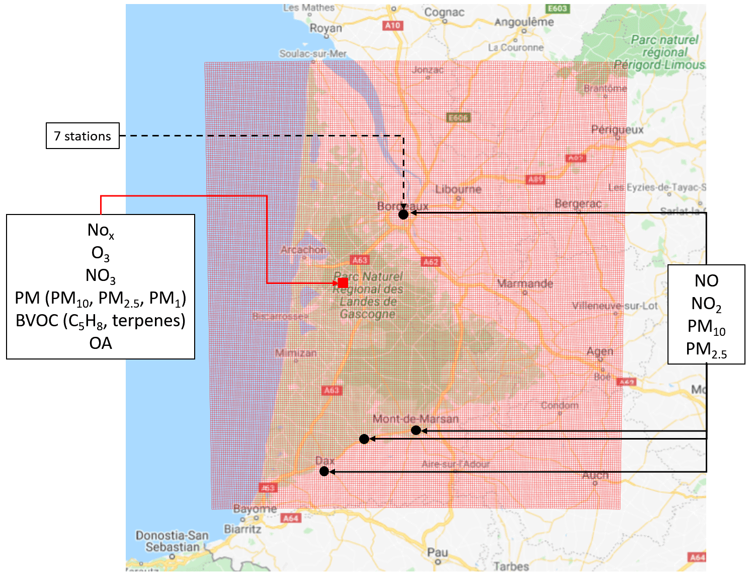
Figure 1 Measurements and monitoring stations in the Landes region and the high-resolution simulation domain (horizontal resolution of 1 km). Black dots represent where the air quality stations used are located, and the red circle shows the main measurement site at Salles-Bilos. Note that the northern point located in the city of Bordeaux includes seven stations (not shown separately because of their proximity). © OpenStreetMap contributors 2022. Distributed under the Open Data Commons Open Database License (ODbL) v1.0.

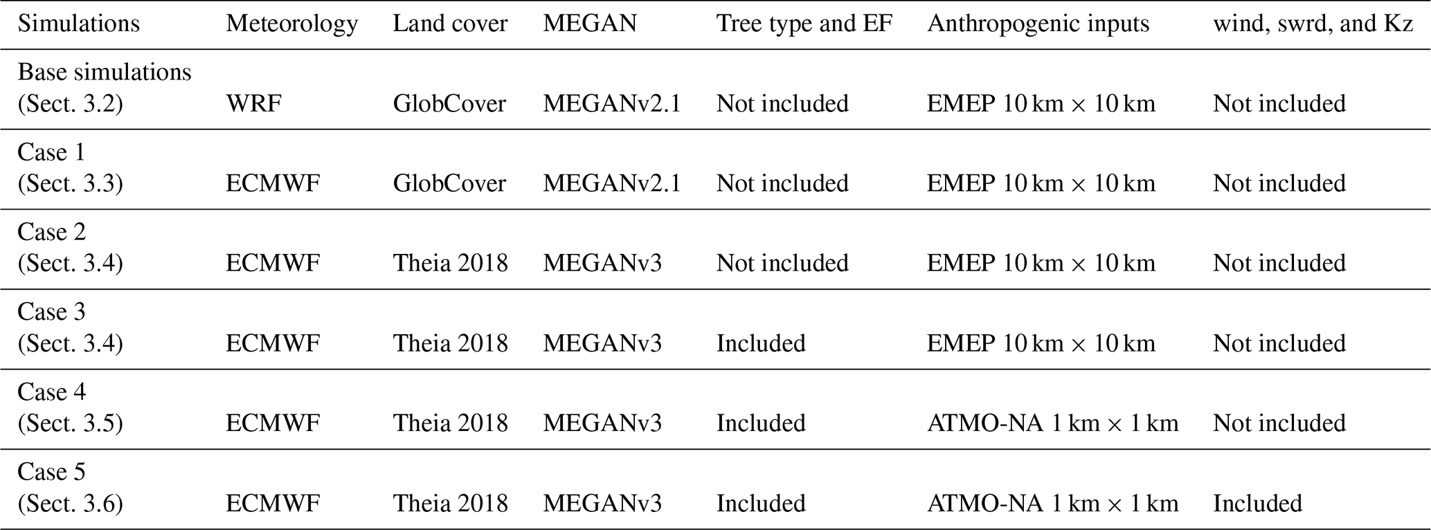
Table 1 Summary of changes in each test case. Each change is explained in more detail in Sects. 3.1 through 3.6. The “tree type and EF” column refers to changes in tree type inputs and their respective emission factors. The “wind, swrd, and K_z” column refers to the test case in which the inside-canopy wind speed, shortwave radiation, and vertical exchange coefficient parameters are modified. For each case the section of this paper in which the changes are explained is mentioned in the first column.

2.1 Characteristics of the main measurement site and measurements performed

The measurements site is located at Salles-Bilos (44${}^{\circ }{\mathrm{29}}^{\prime }{\mathrm{39.69}}^{\prime \prime }$ N, 0${}^{\circ }{\mathrm{57}}^{\prime }{\mathrm{21.75}}^{\prime \prime }$ W, 37 m a.s.l), about 50 km southwest of Bordeaux. It is located in the middle of the Landes forest (Fig. 1), a large forest consisting mainly of maritime pine (Pinus pinaster) trees. The forest parcels are interspersed with agricultural fields, and their character can change from year to year. The specific parcel where the measurements took place consists of pine trees planted in 2004. The height of the trees was around 10 m in 2017. Regarding biogenic emissions, the site is quite homogeneous in terms of tree types since the vast majority of the trees in the surrounding area are maritime pine. However, as mentioned above, since the forest is formed in parcels, the density of the forest and the geographical distribution of these emissions have a certain degree of heterogeneity; parcels can become agricultural fields or be replanted with pine trees, resulting in pine trees with different ages.

The intensive field campaign was carried out just next to the Salles-Bilos ICOS station, part of the European ecosystem monitoring network, where detailed measurements of greenhouse gases and meteorological parameters are obtained at 15 m above the ground on a measurement tower above the forest canopy (ICOS, 2023; Moreaux et al., 2011). During the LANDEX campaign, a large set of gaseous and aerosol measurements was added inside the forest canopy at 6 m height (Bsaibes et al., 2020; Mermet et al., 2021). For the purpose of this study, among gaseous species the measurements of O₃, nitrogen oxides (NO_x), and biogenic volatile organic compounds (BVOCs) will be used, and among the particulate compounds, the concentrations of PM₁₀, PM_2.5, and organic aerosols will be considered. A summary of the measurements used at this site is shown in Fig. 1.

O₃ measurements were performed inside the forest canopy, with the APOA-370 (HORIBA) UV absorption instrument using a temporal resolution of 5 min.

NO and NO₂ measurements were performed by chemiluminescence using an APNA-370 (HORIBA) with a resolution of 5 min and the same height as the O₃ measurements. As this measurement method is not specific for NO₂, the resulting NO₂ measurements may be overestimated, especially for background conditions when much of the concentration of NO_y species is oxidized.

VOCs were measured with an ensemble of different instruments (Mermet et al., 2019; Bsaibes et al., 2020; Mermet et al., 2021). A PTR-Tof-MS (proton-transfer-reaction time-of-flight mass spectrometer) allowed for the measurement of the total concentration of terpenoids (isoprene, monoterpenes, and sesquiterpenes) below the forest canopy at the same height as the previous measurements (around 6 m). Another PTR-Tof-MS was utilized for measurements above the canopy (results for these measurements were not available to the authors of this paper). In addition, gas chromatography–mass spectrometry (GC-MS) measurements were also performed for characterizing BVOC speciation. In this work, the sum of the terpene species resulting from these measurements and the individual concentrations of α-pinene, β-pinene, limonene, and ocimene are all used. Since the purpose of this article is to focus on organic aerosol formation from biogenic compounds and the effect of anthropogenic VOCs on the atmospheric chemistry of the region is limited, anthropogenic VOC measurements are not explored.

Attempts to measure radical species were also made, specifically for OH (using a FAGE instrument from the PC2A partner; Amedro et al., 2012) and NO₃ (IBBCEAS technique from the LISA laboratory, Univ. Paris-Est Créteil, Fouqueau et al., 2020). Because of technical problems, the measurements for OH were not available to be used in this paper. The observed NO₃ concentrations were too low to produce a detectable signal on the instrument; therefore, they were considered to be below the detection limit of the instrument, i.e., below 3–5 pptv.

Particulate matter was also measured during the campaign. PM₁₀, PM_2.5, and PM₁ concentrations were measured using a traditional tapered element oscillating microbalance–filter dynamics measurement system (TEOM-FDMS) (implemented by EPOC) and a FIDAS 200 analyzer (deployed by INERIS), which measures total aerosol concentration in the range of 0.18–100 µm (with three measuring ranges). INERIS also utilized an aethalometer at the same time as the FIDAS in order to measure the black carbon (BC) concentrations. They identified a strong biomass burning episode (on 5 to 6 July) near the measurement site, producing a peak of BC with concentrations as high as 80 µg m⁻³. The simulation of fire episodes using inputs from satellite data is implemented in CHIMERE, but this option was not activated for the runs performed in this study. Therefore, as SOA buildup from biomass burning is not the aim of this paper, this peak has been removed from the particulate matter (PM) data produced by the FIDAS.

A high-resolution time-of-flight aerosol mass spectrometer (HR-ToF-AMS, Aerodyne Research Inc.; DeCarlo et al., 2006) was used in order to measure the bulk chemical composition of the non-refractory fraction of the aerosol operated under standard conditions (i.e., temperature of the vaporizer set at 600 ^∘C and electronic ionization (EI) at 70 eV) with a temporal resolution of 8 min. The concentration of organic aerosol in the PM₁ fraction resulting from this instrument is used in this study.

It should be mentioned that all the measurements used in this work were performed inside the canopy, with the exception of meteorological parameters, which were measured both inside and above the canopy. For meteorological parameters, the above-canopy measurements have been used.

2.2 Other measurement data

The latest version of the E-OBS dataset (Cornes et al., 2018) was used for large-scale meteorological validations for the European and the French domains (see Fig. S1 in the Supplement). These data provide daily regridded information for temperature (daily average, minimum, and maximum), wind speed and direction, relative humidity, precipitation, and solar radiation for around 5000 stations for temperature-related variables and around 1800 for other parameters covering the present-day period going back to 1950s. The data can be downloaded in a regridded format (with a 0.25^∘ × 0.25^∘ horizontal resolution) or as point data (as in the data for each station); the second option is used in this study.

For more comparisons, data from 10 air quality monitoring stations from the ATMO network were also included. The location of these stations, generally at the edge of the forest, is shown in Fig. 1. The measurements available for most of these stations include nitrogen oxides (NO and NO₂) and PM (PM₁₀ and PM_2.5) mass concentrations. These datasets were provided by the local air quality monitoring agency, the ATMO-NA (Atmo-Nouvelle-Aquitaine, 2023); information on the instruments used for the measurements is provided on their site, and historic data are provided upon request. The data cover the entire period of the campaign.

3 The modeling chain

In this section, the reference simulation and sensitivity tests will be presented in detail, in each case documenting the choices made for the changes. The parameters common to all sensitivity tests are explained in Sect. 3.1. After the description of the base simulation (Sect. 3.2), Sect. 3.3 through 3.6 describe sensitivity tests in terms of their changing inputs and variable calculations. Keep in mind that each modification is added on top of the previous ones. The implemented changes are indicated in Table 1.

3.1 The CHIMERE chemistry transport model

The CHIMERE offline regional chemistry transport model (Menut et al., 2013) was developed initially in the early 2000s in order to simulate the concentrations of gaseous species (especially O₃). Later on, a module for the simulation of particulate matter (Pun and Seigneur, 2007; Bessagnet et al., 2008) was added to the model. The model is currently used extensively in air quality monitoring and forecasts for both research and operative purposes at regional and hemispheric levels (Cholakian et al., 2019b; Lachatre et al., 2019; Trewhela et al., 2019; Lapere et al., 2020). It has also been used in many model intercomparison studies, as well as model–observation comparisons within multi-model experiments, for example to investigate European particulate matter trends (Ciarelli et al., 2019). Mandatory input information includes meteorological fields, land cover parameters, biogenic and anthropogenic emissions factors, and boundary and limit conditions. Having access to these data, CHIMERE then simulates 3D concentration and deposition fields for a list of gaseous and size-resolved particulate species, depending on the selected chemical scheme. In this study, the 2017 version of the model has been used (Mailler et al., 2017). In the following section, information about the reference parametrization is provided.

3.2 Base case simulation

The simulations conducted in this study were performed on three domains: a continental domain with a horizontal resolution of 25 km, covering all of Europe and northern Africa (Fig. S1), an intermediary nested domain focused on France with a horizontal resolution of 5 km (Fig. S1), and a 1 km horizontal resolution domain focused on the Landes forest nested inside the intermediary domain (Fig. 1). The vertical resolution of the simulations is the same for each domain, 15 levels starting from 13 m to about 12 km (a.s.l.). Only for the canopy parametrization case (Sect. 3.6) were the vertical levels modified. The simulations were performed for the period of 1 June 2017 to 20 July 2017, with a spinup period of 5 d.

The SAPRC-07A (Carter, 2010) chemical scheme has been used for all the simulations since it provides more details for the terpenoid oxidation than the previously used MELCHIOR scheme. The aerosol size bins are the same for all simulations, a 10-bin logarithmic sectional distribution in a range of 40 nm to 40 µm. The chemical speciation of aerosols contains EC (elemental carbon), nitrates (NO${}_{\mathrm{3}}^{-}$), sulfates (SO${}_{\mathrm{4}}^{\mathrm{2}-}$), ammonium (NH${}_{\mathrm{4}}^{+}$), primary organic aerosols (POAs), secondary organic aerosols (SOAs), dust, sea salt, and PPM (primary mineral particulate matter that does not belong to the previously mentioned groups).

The selected SOA scheme allows differentiating between about 10 surrogate species of semi-volatile BVOC oxidation products with different composition, volatility, and solubility that have been created in a single oxidation step (Pun and Seigneur, 2007; Bessagnet et al., 2008). It takes into account an initial oxidant attack from OH, O₃, and NO₃. The scheme has been used and evaluated on multiple occasions (Lemaire et al., 2016; Cholakian et al., 2018, 2019a). Since this study relies heavily on SOA formation and comparison of this species to measurements, a brief introduction of this scheme will be provided here. The scheme is based on Odum et al. (1996), a simple two-product scheme with the advantage of being numerically light. In this scheme it is considered that the oxidation of BVOCs results in the formation of semi-volatile products with a yield specific to each BVOC family. Some BVOCs consist of specific species (isoprene, α-pinene, β-pinene); others are surrogate groups consisting of similar species lumped together (ocimene, limonene, sesquiterpenes, etc.). As mentioned above, it considers only one step of oxidation for the BVOCs. Assuming a homogeneous mixture, Raoult's law is applied combined with the Pankow theorem (Pankow, 1987), resulting in the calculation of the SOA production yield. The scheme is explained in more detail in Pun and Seigneur (2007). The oxidation reactions that are applied for the production of semi-volatile VOCs have been updated in order to take into account more recent (and more detailed) reactions and reaction rates. The values given on the Carter (2019) site (following Carter, 2010) were used in order to update the reaction rate constants of the BVOCs mentioned above with OH, O₃, and NO₃. The SOA yields have been kept the same as what is provided in Pun and Seigneur (2007), Bessagnet et al. (2008), and the CHIMERE (2023) documentation. We have also included the reactions of BVOCs with different oxidants in the Supplement (refer to Sect. S8).

Boundary and initial conditions are taken from climatological simulations of LMDz-INCA3 (Hauglustaine et al., 2014) for gaseous and particulate species and GOCART (Chin et al., 2002) for dust concentrations.

For each CHIMERE simulation domain, the meteorological parameters were obtained by running the Weather Research and Forecast (WRF) model (version 3.9.1.1; Wang et al., 2015) on the same domain and with the same horizontal resolution with the NCEP large-scale input data (National Centers for Environmental Prediction/National Weather Service/NOAA/US Department of Commerce, 2000). Several model configurations have been tested in the WRF model. A comparison of the model outputs with the E-OBS database (Cornes et al., 2018) and the measurements obtained at the Salles-Bilos measurement site was conducted for all the performed meteorological runs. For the base simulations, the WRF configuration showing the best comparison results (as detailed in Sect. S2) with the Salles-Bilos site was chosen (see Fig. 2 for time series and statistical information). All the parametrizations tested using WRF are presented in Sect. S2. The WRF parametrization that is retained is a two-way triple-nested run with a WSM six-class graupel microphysics scheme, Kain–Fritsch cumulus scheme, RRTMG scheme for both shortwave and longwave radiation, Noah-MP land surface, MYNN surface layer option, MYNN third-level TKE boundary layer height option, topological wind, urban physics, lake physics options, and nudging options activated. These options are all described in detail in the user guide for the WRF model (Wang et al., 2015).

The GlobCover (Arino et al., 2008) dataset with a resolution of 300 m × 300 m was used for the land cover parameters. Bearing in mind that the forest is structured into parcels and that some parcels can be transformed into agricultural fields, changing this database to a more recent one was considered to be beneficial for this study (see Sect. 3.4).

Biogenic emissions are provided by a reduced online version of the MEGAN (Guenther et al., 2012) model that has already been integrated into the CHIMERE model. For the base simulations, version 2.1 of the MEGAN model has been used. This version of MEGAN comes with pre-calculated BVOC emission factors for isoprene, α-pinene, β-pinene, limonene, ocimene, humulene, and β-caryophyllene (including the leaf area index (LAI) fields) with a horizontal resolution of 0.008^∘ × 0.008^∘. Therefore, any land-cover-related changes in the model will not affect the BVOC emission factors. These emission factors were calculated using the GlobCover land cover database. In a later sensitivity test (Sect. 3.4), a more recent version of the MEGAN model has been tested. Using this version, we have the possibility of recalculating the BVOC emission factors by changing the land cover, the vegetation-specific emission factors, and the LAI. A more detailed explanation of this model and its use is provided in Sect. 3.4.

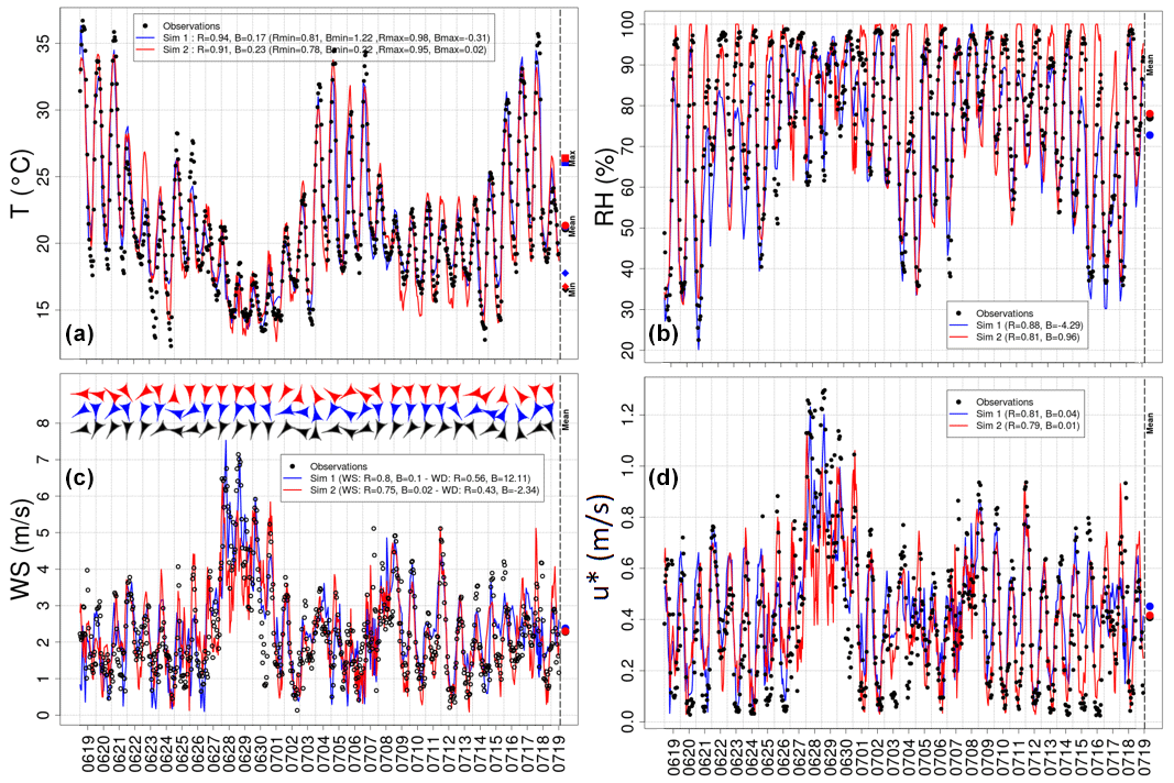
Figure 2 Meteorological comparisons for the two meteorological inputs. The blue series (SIM1) shows the ECMWF simulations, and the red series (SIM2) shows the WRF outputs. Statistical information is provided in the legend for each figure (R is the correlation coefficient, and B is bias (simulation–observation)). The name of each parameter is written on the side of each panel, and the points on the right side of each panel show the average data for each series. The comparisons are performed for the 1 km domain and for the Salles-Bilos measurement site. The comparisons are performed at surface level. Panels (a)–(d) show temperature (a, marked as T, in ^∘C), relative humidity (b, marked as RH, in %), wind speed and wind direction (c, Ws is wind speed in m s⁻¹, and directions are shown at the top of each day), and friction velocity (d, marked as u* in m s⁻¹). More information about all of the WRF simulations and the one that was chosen to be presented here (WRF3) is given in Sect. S2.

Anthropogenic emissions were taken from the EMEP (EMEP/EEA, 2022) emission database with a 10 km resolution for the year 2014. The emissions in this database for the years 2014, 2016, and 2017 were compared, and no major differences were observed in the levels of anthropogenic emissions between these years for this specific region (the data can be directly compared using the EMEP emissions data center, accessible from EMEP, 2023). The reason for using the 2014 emissions is explained in detail in Sect. 3.5, where a local high-resolution emission database is tested.

It is worth mentioning here that the CHIMERE model does not have an integrated forest canopy model; therefore, the model, while taking into account the biogenic emissions and the land cover information of the forest in different modules (for example for calculating the deposition of atmospheric species), will not take into account the dynamic physical changes introduced by the forest canopy into the concentrations of chemical species in the first two vertical layers of the simulations. These effects and the changes made in the model in order to address them are presented in detail in Sect. 3.6.

3.3 Meteorological inputs

In addition to the tested WRF parametrizations, another series of meteorological inputs was tested using the ECMWF high-resolution 3-hourly forecast dataset (Owens and Hewson, 2018). The global version of the ECMWF data (with lower resolution) is used for the continental domain, while for the other two domains the high-resolution (10 km) ECMWF run is used. The comparisons of the measurements from the Salles-Bilos site to a simulation run with the ECMWF meteorological inputs are shown in Fig. 2, and a comparison is also made using the WRF parametrization mentioned in Sect. 3.2. Before commenting on this comparison, we first briefly present the meteorological situation during the campaign, which is depicted by both models in a similar way. Rainfall events (not shown in Fig. 2) occurred between 26 June and 3 July and also in the 8 to 13 July 2017 period and were associated with low solar irradiance (<750 W m⁻²), mild summer temperatures (<25 ^∘C), high relative humidity (>75 %), and moderate winds. These periods are defined as “low-oxidation” periods. Two episodes of sunny conditions were observed during the campaign, i.e., from 4 to 7 July and then from 14 to 18 July. These periods were characterized by higher temperatures, relative humidity below 50 % (during the day), low wind speeds (<3 m s⁻¹) and friction velocity (<0.3 m s⁻¹), and no precipitation. These periods were favorable to plant emissions and strong oxidant formation and are called periods of “strong oxidation”. It appears that models adequately describe the broad meteorological situation during the campaign summarized by Mermet et al. (2021).

While both meteorological runs represent the measurement site in the smallest domain quite accurately, the ECMWF run shows a better representation for the two bigger domains for all of the tested parameters (mean, maximum, and minimum temperature; wind speed and direction; and relative humidity; see Sect. S2), thus providing more accurate meteorological patterns at the boundaries of the high-resolution domain. As for the high-resolution domain, the daily mean and maximum temperature values are well simulated in both meteorological inputs (Fig. 2a). However, both models have shortcomings in the representation of daily minimum temperature values: this problem is more significant in the WRF simulations (for daily minima, a bias (simulation–observation) of +0.22 and +1.22 ^∘C is observed in the ECMWF and WRF data, respectively). The wind speed simulations are accurate in both runs (Fig. 2c), while the wind direction is more representative of the domain in the ECMWF simulations. The friction velocity (u*, Fig. 2d) shows the same pattern and is well represented in both datasets; however, the nighttime minimum is better represented in the WRF simulations. Precipitation and the Bowen ratio β (the ratio of heat flux to moisture flux near the surface) were also compared and are presented in Sect. S3.

3.4 Land cover, tree type, and tree-specific emission factors

Since the forest is divided into parcels and goes through annual changes, it is important to use an up-to-date source of information on forest cover and density when performing high-resolution simulations. To this end, a detailed comparison of existing land cover data was conducted. It should be noted that trees are lumped into two main functional groups in most land cover databases: broadleaf trees and needleleaf trees. In addition to tree density (which varies upon the selected database), the broadleaf–needleleaf distribution is also a specific parameter of land cover datasets. This is why all databases in this exercise have been examined in terms of their total tree density (this section) and with respect to the BVOC emissions they induce, taking into account the broadleaf–needleleaf distribution (see Sect. 3.5).

In particular, from this point on, a more recent version of MEGAN (MEGAN3.0; Guenther et al., 2018) has been used that provides the possibility of modifying the land cover and the emission factors attached to different tree types and different regions. Therefore, all of the modifications mentioned here were made both in MEGAN and in CHIMERE simultaneously. We performed two separate test cases: one for changing the land cover data and another for changing the regional tree species and the emission factors tied to specific trees. Both of these modifications result in changes in the general BVOC emission factors; therefore, they are presented in the same place.

In the first test case, we considered the datasets provided by CHIMERE and WRF models and compared them to several other more recent or regionally specific datasets. CHIMERE allows the use of two datasets for land cover information: the GlobCover dataset (Arino et al., 2008), as selected for the base simulation, and the USGS dataset (Gutman et al., 2008). As for the WRF model, it provides the option of using MODIS (Giri et al., 2005) or USGS data. Also, the forest cover density information made available in MEGAN was also included in our comparisons. In addition to these data, three databases of major interest were added to our comparison (Fig. 3b, c, and d).

First, we considered the Copernicus database (Copernicus, 2023), which provides (among other parameters) information about the tree cover density over Europe for the years 2012 and 2015 with a horizontal resolution of 20 m. The Copernicus database also provides forest changes across Europe between the years 2012 and 2015. These changes are, on average, about +30 % forest growth in grid cells where the changes were positive and about −40 % in grid cells where the changes were negative. Given these important changes, only the most recent (2015) dataset was considered. This database was regridded to our 1 km resolution domain to have a common grid for comparisons (Fig. 3e).

We also collected data from the IGN (Institut national de l'information géographique et forestière), which provides detailed information on forest density (via the BDForêt database) and general land cover information (via the BDTopo database) in France. These data were downloaded from the IGN data portal (IGN, 2023a) for three administrative departments (Landes (40), Gironde (33), and Lot et Garonne (47)) in order to cover the entire Landes forest. Both the BDForêt and the BDTopo databases have high resolution (around 20 m); temporally, the BDTopo database is for the year 2017 (published in 2019), while the BDForêt database was updated in 2018 with data from 2017. The data for both databases were processed into a format that is usable in CHIMERE (i.e., projection of shapefiles onto a regular netcdf grid) and then regridded to the 1 km domain. This provides us with two more sources of comparison shown in Fig. 3f and g (denoted as BDForêt and BDTopo).

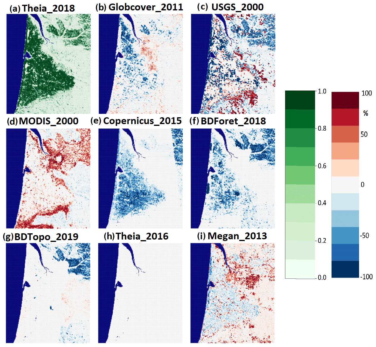
Figure 3 Forest density comparisons for different land cover databases. The name of each database is shown at the top of each image. The forest density is shown for the Theia2018 dataset in (a); the rest of the panels show the percentage differences between each database and the Theia2018 dataset. Two scales are provided for the figure. The first scale (shades of green) corresponds to the reference case (a), and the second scale shows the differences between the reference case and the indicated dataset (b through i).

There is also a land cover dataset provided by the French National Institute of Agriculture, Alimentation, and Environment (INRAE, Institut national de recherche pour l’agriculture, l’alimentation et l’environnement), called the Theia dataset (IGN, 2023b). This dataset includes several types (reflectance, snow mask, water level, etc.) of information gained from remote sensing observations of the Earth, including land cover data. The dataset was realized first in 2016 and then updated in 2018 with a horizontal resolution of 20 m. Both the 2016 dataset and the 2018 dataset are presented in this study (Fig. 3a and h). It is important to know that the base data used in order to generate the Theia datasets, apart from satellite information, is the BDTopo database presented in the previous paragraph. Comparing the two Theia datasets (2016 and 2018), a difference of 29 % is seen when conifer tree density is involved (although differences in total tree cover are small).

Since Theia 2018 is the most recent source of information we could acquire for the region at this time and is based on several independent data sources, it was taken as a reference in Fig. 3a. The upper-left frame shows the Theia 2018 tree cover density for the Landes forest in shades of green. It draws a strongly delimited triangle of dense forested area on the domain, which becomes irregular in the southern part of the domain and near the coastline. The other frames show the relative difference in each database with respect to Theia 2018. It can be seen that there are practically no differences between Theia 2018, BDTopo, and Theia 2016 (average density over the forest is 68.32 %, 68.95 % and 68.20 %, respectively) and only slightly lower densities in the BDForêt and MEGAN databases (63.2 % and 58.29 %, respectively), while strong differences appear with the MODIS, GlobCover, Copernicus, and USGS data. MODIS proposes a much higher forest density than Theia, especially in and around the edge of the Landes forest. A possible reason for this could be the data being outdated (the MODIS version used here dates from 2000) or the lower resolution of MODIS (1 km × 1 km) compared to the others. The Copernicus database shows a consistent underestimation of the forested area over the Landes forest. The same is true for the GlobCover database to a lesser degree. This is probably because its resolution is higher than MODIS, but it is still outdated (2000s). The USGS database shows either a strong overestimation or an underestimation for different 1 km grid cells. Since this database is quite old (2003), the changes between forest and agricultural fields could be responsible for these discrepancies. From this point on, the Theia 2018 land cover database is used both in CHIMERE and in MEGAN.

The second step in this section is to analyze the estimation of the BVOC emission factors when tree types in the region and tree-specific emission factors are changed in MEGAN. The BDForêt database mentioned above provides more detailed information about distribution of tree species inside the Landes forest as well as their density. It was considered necessary to modify the tree type distribution in the MEGAN v3 model since originally it assumes 28 % of maritime pine coverage for the Landes forest, while the BDForêt database shows around 95 % of the same species. The reason for this discrepancy is that MEGAN considers an average tree species distribution for western European forests up to 300 km from the Atlantic coast, which does not take into account the specificity of the Landes forest. Therefore, modifications were made in the MEGAN v3 model inputs in order to (i) create a specific ecosystem for the Landes forest containing 95 % of maritime pines and (ii) modify the emission factors for the maritime pine to experimental values obtained during the LANDEX campaign (Elena Ormeno, personal communication, 11 June 2019). The emission factor for maritime pines was measured on the canopy and also on the litter levels during the same campaign this study simulates. The measurements resulted in an average of 3.8 µg g⁻¹ h⁻¹ at the canopy level and an average of 1.6 m g g⁻¹ h⁻¹ at the litter level of total monoterpene emissions (individual emission factors for BVOCs are also available upon request from the source mentioned in the article). The values provided here for the canopy and the litter are almost 3 times and 2 times higher, respectively, than the original values used in MEGAN v3. The resulting emission factors were integrated into MEGAN v3. Total emission factors per BVOC were generated and integrated in CHIMERE, and a sensitivity case was run with this new configuration. The resulting emissions of isoprene and the sum of terpenoids (monoterpenes and sesquiterpenes) using these new emission factors are shown in Fig. 4 for both sensitivity tests detailed here. Figure 4 justifies a posteriori the importance of this sensitivity test, since the emissions of isoprene have dropped by about half, while the emissions of terpenoids have increased significantly, by about a factor of 2. In Sect. 4.1, we will explore the effect of these emission changes on BVOC concentrations and compare the results to observations. Taking into account that maritime pine emits terpene and that the forest is mostly covered by this species, these emissions are more realistic for the Landes forest than the original ones. Monoterpene emissions (averaged over the entire forest) increase by around 33 % when only land cover is changed (Fig. 4b), while emissions of isoprene decrease by around 30 % when there is a land cover data change (Fig. 4e). For the region being studied here it is important to notice that the effect of changing the type of trees and the experimental emission factors for these trees is more important for the emission of monoterpenes, while the change caused by modifying the land cover seems to be more important for isoprene emissions.

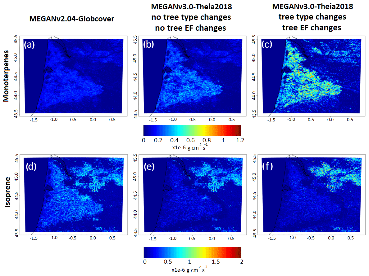
Figure 4 Changes to monoterpene (first row, a–c) and isoprene (second row, d–f) emissions in base case conditions (left column, a and d), changing only the land cover (middle column, b and e), and when both the land cover and MEGAN version are updated (right column, c and f). For each species one scale is provided under the three panels; keep in mind both scales should be multiplied by $\mathrm{1}\times {\mathrm{10}}^{-\mathrm{6}}$ (the unit for all panels is g cm⁻¹ s⁻¹).

It should be taken into account that a test was run by replacing the LAI used in the model with the Copernicus 1 km horizontal resolution global LAI-v2 databases (Copernicus Land services, 2023) for the year 2017, leading to no significant changes in the results of the simulations compared to when the LAI implemented in CHIMERE (from MEGAN v3) is used.

3.5 Anthropogenic emissions

For the reference simulation, anthropogenic emissions from the EMEP inventory that have a horizontal resolution of 10 km are used. This is assumed to be precise enough because the region has, at least when it comes to the forest, a low anthropogenic footprint. However, the transport of recently emitted compounds to the forest by the anthropized areas around the forest (including large cities such as the Bordeaux metropole to the north and smaller ones such as Dax to the south, as well as industrial sites located to the west and northwest of the forest) and motorway traffic passing through the forest need to be taken into account in more detail. To this end, in CHIMERE we have implemented the kilometric emission dataset provided by the regional air quality agency (ATMO-NA). This fifth sensitivity case revolves around changing the anthropogenic emissions from the reference EMEP emissions to the emissions provided by ATMO-NA. This modification, in addition to providing anthropogenic emissions with greatly increased horizontal resolution, has the advantage of being prepared from bottom-up data specific to this area. The comparison of these two emission datasets is shown in Sect. S4. In summary, the two databases show comparable emissions for all species, presenting the highest average bias (simulation–observation) for SO_x of around 20 %, with dominant SNAP sectors being always the same for each species group between the two emission inventories. It should be noted that the emissions provided by ATMO-NA are for the year 2014; therefore, in order to have consistent emission inventories, we have used the 2014 EMEP emission inventory for this test. The total national NO_x emissions differ around 9 % between 2014 and 2017 on average in the EMEP dataset.

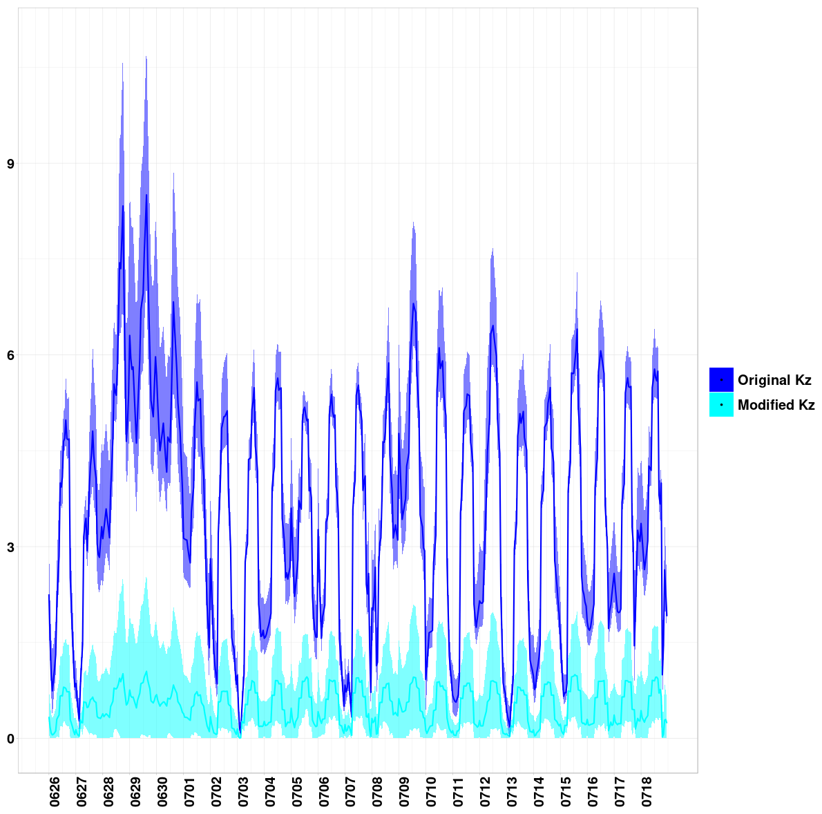
Figure 5 Changes in K_z (m² s⁻¹) between the first and second model layer in test cases without any modifications and the test case in which the K_z corrections are applied. The lines are for the grid cell corresponding to the Salles-Bilos site, and the envelope corresponds to grid cells in the 11 km × 11 km area surrounding the site. The reasoning for showing 11 km × 11 km is given in Sect. 4.

3.6 Vertical diffusion, wind speed, and shortwave radiation corrections

Since the CHIMERE model does not have a coupled canopy model, it cannot take into account the physical effects that the forest canopy might exert on concentrations of chemical species. The last sensitivity case is based on the corrections of the effects that the canopy can have on the simulation of physical parameters such as vertical diffusion (K_z, m² s⁻¹), wind speed, and shortwave radiation in the model (this will be referred to as the final test case from here on).

While the effect of the canopy on BVOC emissions is already taken into account in the MEGAN model, the effects of the canopy on wind speed and vertical diffusion inside the forest are not simulated in the CHIMERE model. In a large-scale simulation and outside of comparisons to inside-canopy measurements, this usually does not cause major issues. But since the goal of this work was to understand the atmospheric situation inside the canopy, almost all measurements are performed inside it. Furthermore, simulations performed here are high-resolution simulations; therefore, we have added corrections for the aforementioned physical parameters inside the canopy in order to simulate the physical conditions of the forest more realistically. These modifications will be presented as the sixth sensitivity test, which is theoretically the most realistic one. In this test, a small inconsistency subsists because deposition is only treated in the lowest layer in the model, while it could also affect the second layer that contains part of the canopy.

For this purpose, the vertical diffusion and the wind speed correction suggested by Ogée et al. (2003) and Leuning (2000) implemented within the MUSICA canopy model have been integrated into the fine domain of our simulation for the model grid cells where the forest density is higher than 70 %. The MUSICA canopy model is a 1D model developed in the early 2000s; it has been detailed by Ogée et al. (2003). The case study presented in the aforementioned study is also for the Landes forest and has been validated by comparisons against measurements.

In the standard version of the CHIMERE model, the vertical diffusion (K_z) is calculated by the parametrization suggested by Troen and Mahrt (1986). Depending on the atmospheric stability (determined by the Monin–Obukhov length), the K_z can relate to u* in different ways depending on atmospheric stability. The equation for K_z is

$$\begin{array}{}\text{(1)}& K_z=k{w}_{\mathrm{s}}{\displaystyle \frac{z}{h}}(\mathrm{1}-{\displaystyle \frac{z}{h}}{)}^{\mathrm{2}},\end{array}$$

where k represents the von Kármán constant and the factor w_s is calculated differently depending on the atmospheric stability.

$$\begin{array}{}\text{(2)}& {\displaystyle }& {\displaystyle }\text{stable conditions}:w_{\mathrm{s}}={\displaystyle \frac{u_{*}}{(\mathrm{1}+\mathrm{4.7}\frac{z}{L}))}}\text{(3)}& {\displaystyle }& {\displaystyle }\text{unstable conditions}:w_{\mathrm{s}}=(u_{*}^{\mathrm{3}}+\mathrm{2.8}e{w}_{*}^{\mathrm{3}}{)}^{\frac{\mathrm{1}}{\mathrm{3}}}\end{array}$$

Here $\frac{z}{L}$ is the ratio of altitude to the height of the boundary layer, u_* is the friction velocity, and L is the Monin–Obukhov length. A more detailed explanation of the calculation of K_z can be found in the CHIMERE model documentation (downloadable from the CHIMERE, 2023, site.).

In this work we have added the diffusivity and horizontal wind correction factors (ϕ_w(ξ) and ϕ_h(ξ), respectively) using the references mentioned above:

$$\begin{array}{}\text{(4)}& {\mathit{\varphi }}_{\mathrm{w}}\left(\mathit{\xi }\right)=\left\{\begin{array}{ll}& \mathrm{1.25}(\mathrm{1}+\mathrm{3}\left|\mathit{\xi }\right|{)}^{-}\frac{\mathrm{1}}{\mathrm{3}},-\mathrm{2}⩽\mathit{\xi }<\mathrm{0}\\ & \mathrm{1.25}(\mathrm{1}+\mathrm{0.2}\mathit{\xi }),\mathrm{0}⩽\mathit{\xi }<\mathrm{1}\end{array},\right.\end{array}$$

$$\begin{array}{}\text{(5)}& {\mathit{\varphi }}_{\mathrm{h}}\left(\mathit{\xi }\right)=\left\{\begin{array}{ll}& (\mathrm{1}+\mathrm{16}\left|\mathit{\xi }\right|{)}^{-\frac{\mathrm{1}}{\mathrm{2}}},-\mathrm{2}⩽\mathit{\xi }<\mathrm{0}\\ & (\mathrm{1}+\mathrm{5}\mathit{\xi }),\mathrm{0}⩽\mathit{\xi }<\mathrm{1}\end{array},\right.\end{array}$$

where ξ the stability factor is calculated by

$$\begin{array}{}\text{(6)}& \mathit{\xi }=\left\{\begin{array}{ll}& \frac{h_{\mathrm{c}}}{L},z<z_{\mathrm{ruf}}\\ & \frac{(z-d)}{L},z\ge z_{\mathrm{ruf}}\end{array},\right.\end{array}$$

where h_c is the canopy height (m), z is the altitude (m), d is the zero-plane displacement for momentum, and z_ruf≈2.3h_c.

In the end, K_z is calculated by the following equation (taking into account the diffusivity correction):

$$\begin{array}{}\text{(7)}& K_z={\mathit{\varphi }}_{\mathrm{w}}k{w}_{\mathrm{s}}{\displaystyle \frac{z}{h}}(\mathrm{1}-{\displaystyle \frac{z}{h}}{)}^{\mathrm{2}},\end{array}$$

and the horizontal wind speed components are multiplied by ϕ_h. The diffusion and wind corrections are affected only in the first level of the model, which has a height of 8 m specifically for this case, and in grid cells with a forest density greater than 70 %; a stability correction is also included at the same time (explained in Ogée et al., 2003).

The changes induced for the vertical diffusion are shown in Fig. 5. The line shows the K_z at the measurement site, and the ribbon around the line shows the regional changes around the measurement site up to a distance of 5 km on each side. The upper panel shows the standard vertical diffusion, and the lower panel shows the corrected K_z. Results indicate a strong decrease of roughly 1 order of magnitude in the vertical exchange coefficient between the first and second model layer when the canopy parametrization is taken into account.

The modification for shortwave radiation penetration inside the canopy comes from Hassika et al. (1997), which itself is a continuation of the work performed by Berbigier and Bonnefond (1995). Both studies revolve around the Landes forest, but they are more general in their formulation. The following variation of Beer's law is used to achieve this purpose:

$$\begin{array}{}\text{(8)}& \mathrm{swrd}\left(z\right)=\mathrm{swrd}\left(\mathrm{0}\right)e^{\frac{-k\times \mathrm{LAI}\left(z\right)}{\cos \mathit{\beta }}},\end{array}$$

where swrd(z) is the shortwave direct radiation at the altitude z, swrd(0) is the shortwave direct radiation above canopy level, LAI(λ) is the leaf area index at the altitude z, β is the zenithal angle, and finally k is the extinction factor, measured to be 0.33 for the Landes forest (calculated by Ogée et al., 2003, using experimental data). In the case of our simulation, we do not need a distribution of shortwave radiation for different altitudes within the canopy but rather a bulk decrease, which we calculate here for the middle of the lower part of the first model layer between 0 and 6 m height (because LAI is supposed to be distributed between 6 and 10 m above ground level). This simulated value can thus be observed at 6 m height at Salles-Bilos. According to visual inspection of the measurement site, most of the LAI is distributed in the last meters of the pine trees in that specific patch of the forest. This equation is also used on grid cells with higher than 70 % tree density. It is also important to take into account that the swrd changes affect only the chemistry modules of the model, and they do this by reducing photolysis frequencies. On the contrary, emissions of BVOCs are not affected by these modifications since the effect of the canopy on the decrease in swrd is already taken into account in the MEGAN model when calculating the BVOC emission factors.

These modifications were added in two steps. First, the K_z and the wind speed modifications are added. Second, the swrd modification is added. Therefore, it was possible to determine the changes made by K_z and wind speed modifications compared to the changes induced by the swrd changes. The changes made to the K_z before and after the correction are shown in Fig. 5.

It is important to keep in mind that this modification has been performed as a sensitivity case and not a functional parametrization for the model. The correction factors for diffusivity and wind speed have been calculated for this measurement site according to the work from Ogée et al. (2003). While they should be usable in other forests, the specific values should be adjusted to the specific conditions there (especially canopy height and LAI). Also, canopy-induced modifications in the vertical diffusion are considered at the top of the first model layer, which is fixed for this case at 8 m height and is thus well within the canopy (which is 10 m high at the measurement site). For the wind speed and radiation, modifications are considered for the middle of the first layer, i.e., at 4 m height.

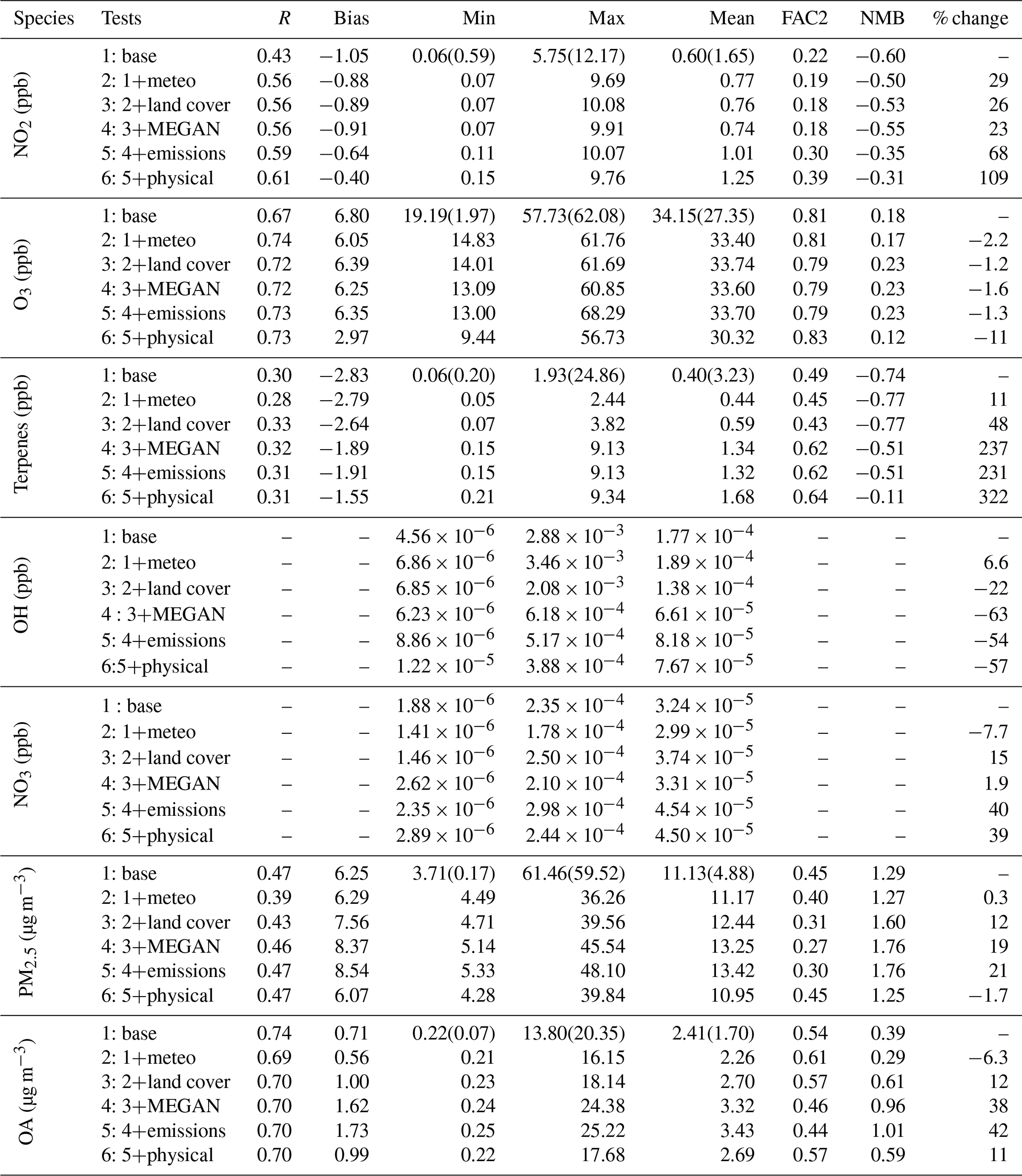
Table 2 Statistical information for test cases showing correlation coefficient to measurements (R, when possible); bias (absolute difference between model and measurement averages); minimum, maximum, and average values (min, max, and mean); fraction of predictions within a factor of 2 of observations (FAC2); normalized mean bias (NMB); and the percentage of change in the mean for each test case compared to the base simulation. When measurement data were available, their value is given in parentheses. The units and the species names are given on the left side of the table. Percentage (%) change indicates the relative change in simulated means with respect to the base case.

4 Effects of the model configuration on simulations of SOA, precursors, and oxidants

In this section, results from a series of sensitivity cases will be discussed, starting from a regional standard configuration of the CHIMERE model and moving to one updated for the local Landes forest conditions. The first primary gaseous species of biogenic and anthropogenic origins will be examined (Sect. 4.1), followed by O₃ as a secondary species (Sect. 4.2), radicals (Sect. 4.3), and finally particulate matter, with a focus on its organic fraction (Sect. 4.4). Changes induced by sensitivity tests will be compared to measurements at the Salles-Bilos site. In Sect. 4.5, the changes to the contribution of precursors and oxidants to BSOA formation will be assessed in the base case compared to the simulation with all the modifications. Keep in mind that whenever changes are discussed in this section, changes in averages over the entire period of each test case compared to average of the entire period of the base case are being discussed.

Several of the species being discussed in the following sections have high local sensitivity depending on the forest coverage of a given location. As well as showing the square in the model where the measurement site is, a range of simulated concentrations in a 11 km × 11 km square around that point is also added to the figures in order to convey the entire local conditions.

In Sects. 4.1 to 4.4, observed and simulated time series at the Salles-Bilos site will first be analyzed. The percentage change in the concentration of different species caused by each sensitivity test compared to the previous one will be indicated. Finally, the effect of the complete set of sensitivity studies on their comparison to observations in terms of bias (simulation–observation), mean error, and correlation will be addressed.

4.1 Biogenic and anthropogenic primary gaseous species

The sum of monoterpenes is the first group of species that we consider here. Measurements from PTR-Tof-MS are compared to the simulated sum of α-pinene, β-pinene, limonene, and ocimene concentrations. The $m/z$ 137 peak as the main fragment of monoterpenes and $m/z$ 81 values as the second-most-important fragment are both taken for the PTR-Tof-MS measurements (refer to Li et al., 2020, 2021, for detailed information about treatment of PTR-ToF-MS measurements). Figure 6 shows a comparison of O₃ and terpene concentrations with measurements in different sensitivity tests (both shown in ppb; NO₂ is shown in the Sect. S5). It should be noted that each of these BVOCs have been compared separately to measurements as well; the comparisons are presented in the Supplement (Figs. S6–S11).

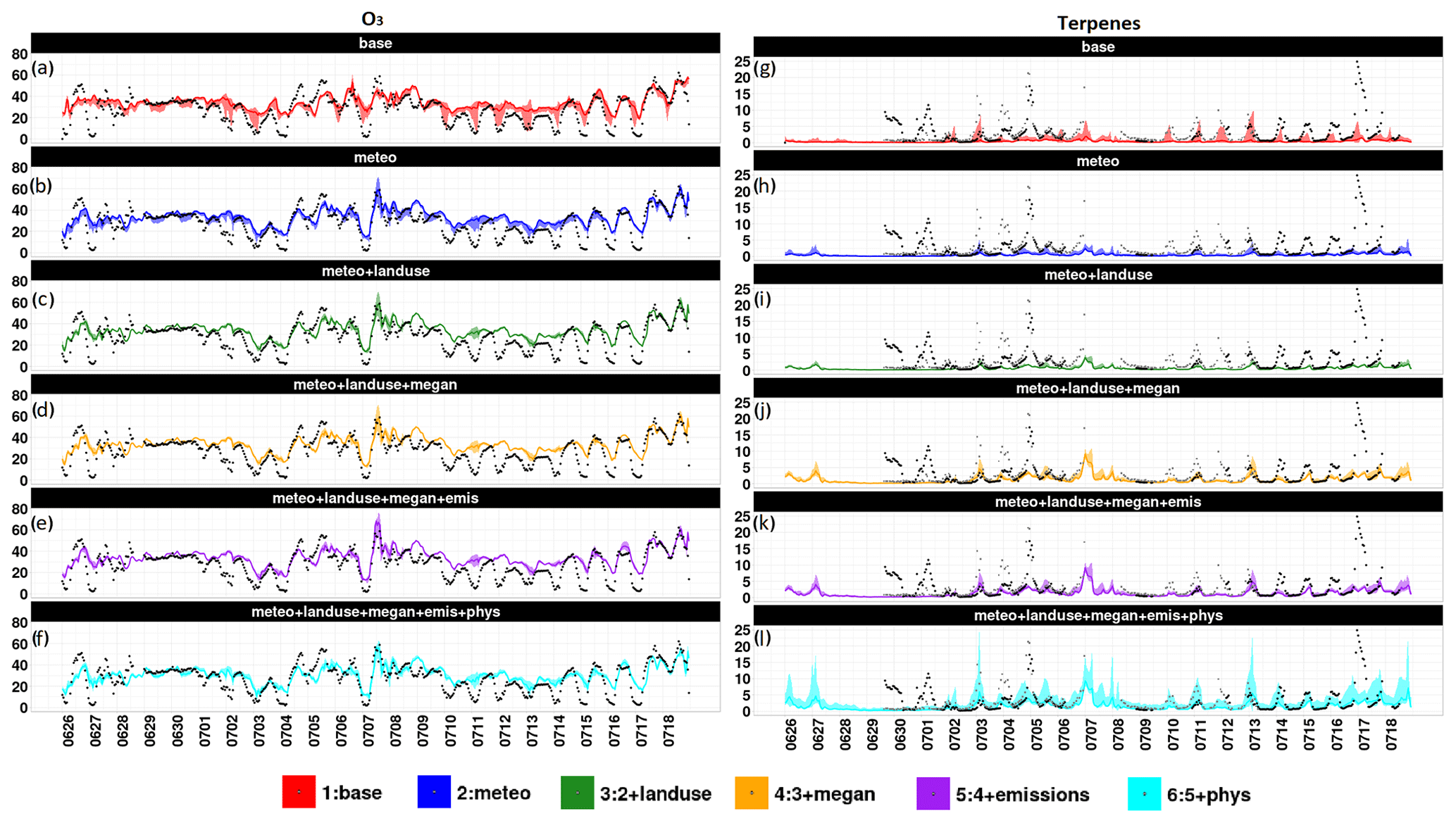
Figure 6 Time series for O₃ and terpene concentrations (all in ppb) for all the sensitivity cases explained in Sect. 3 and Table 2. The color scheme is shown at the bottom. The name of each case is written above each time series. Time series for other species are provided in the Supplement.

Terpene concentrations are source-dependent and enhanced locally; they are more important near emission sources throughout the forest area (Figs. 4 and 10). Observed and simulated terpene concentrations (Fig. 6g–l) show a marked diurnal cycle with increased nighttime levels due to decreased sink processes (less OH and O₃ but more NO₃) and decreased horizontal and vertical dispersion (nighttime wind speeds and exchange coefficients are minimal), as pointed out by Bsaibes et al. (2020) and Mermet et al. (2021). Observed nighttime terpene maxima range between 5 and 25 ppb. The largest concentrations are reached during nights of 2–3, 4–5, and 16–17 July. These peaks generally correspond to lower friction velocity observations (below 0.1 m s⁻¹) and larger temperatures, as pointed out by Bsaibes et al. (2020).

Simulated terpene maximum levels with the base case configuration barely exceed a few parts per billion and can reach up to about 10 ppb in the 11 km × 11 km area around the Salles-Bilos measurement site. The nighttime peaks during 4–5 and 16–17 July are not reproduced, which could probably be explained by an overestimation of friction velocity during these nights (as seen in Fig. 2d). Increased daytime concentrations are simulated during the two hot weather periods (4–8 and 16–18 July).

Some of the sensitivity cases explored in this study cause strong positive changes in the concentrations of terpenes: 11 % when changing land cover inputs, +103 % (always compared to the base case average) when updating biogenic emissions with local emission factors, and +145 % when changing the K_z parametrization. The 10 % increase while changing the land cover is related to the tree density changes in the region; however, it is interesting to keep in mind that changing the land cover may also decrease the tree density in the forest since some parcels were recently turned into agricultural fields. For the measurement cell, tree density increases by around 29 %. The increase in terpenes when updating the biogenic emissions occurs because both the tree types and the tree emission rates for the forest have been rectified in the emissions produced by the MEGAN model. Coherently, this also leads to a decrease (−73 %) in isoprene concentrations, since changing the majority of the Landes forest tree type in MEGAN to maritime pine means that the density of isoprene-emitting trees is significantly reduced. Including the canopy parametrization in the model causes emitted terpenes to be exchanged less between inside the canopy and above the canopy. It also increases the variation in terpene concentrations locally, seen in the larger envelope around the study area as part of the canopy-effect sensitivity case in Fig. 6. The other two test cases show slightly negative effects in terms of the terpene concentrations (−10 % and −2 % for the meteorological test case and the anthropogenic emission test case, respectively). Figure 7 shows the distribution of isoprene and terpene in the base case (Fig. 7a) and the final (Fig. 7b) sensitivity case for the measurement cell compared to the distribution of different monoterpene and sesquiterpene species in the measurements (Fig. 7c). It is important to note that this distribution changes substantially between the base case and the final case, being much closer to the observed distribution after the biogenic emission and land cover modifications. An overestimation of isoprene is still seen in the final case.

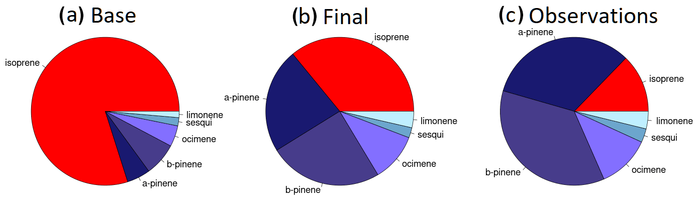
Figure 7 Pie charts of the distribution of BVOCs in the observations, the base case, and the final case. In the species presented here, every species represents only the species named apart from ocimene. Ocimene is the sum of myrcene and ocimene in the model, and the same sum is presented for the measurements.

Finally, and importantly, the different test cases lead to a clear improvement in the average and maximum simulated sum of terpene concentrations (see Fig. 6g–l). In particular, the negative biases are strongly reduced for maximum terpene concentrations, from 14.0 to 22.4 ppb, as compared to 25.2 ppb in the observations. It is also important to keep in mind that in the canopy test case the changes seen in the concentrations come almost entirely from the K_z modifications and not from the modification made to the shortwave radiation.

Following this, simulations of NO₂ as a tracer of anthropogenic emissions are discussed (see Fig. S5 in the Supplement). Observed NO₂ level is at its maximum mostly during the night and early morning hours, reaching peaks between 3 and 7 ppb (for the nights of 2–3, 3–4, 6–7, 15–16, and 16–17 July). Again, this is due to reduced local dispersion, in addition to suppressed NO₂ photolysis, and in spite of lower nighttime NO_x emissions. Its NO₂ changes most in two cases: the anthropogenic emissions test case (+26 %) and the meteorological test case (+20 %). The refined distribution of anthropogenic emissions explains the majority of the first case, as average emissions over the inner model domain increase by only 4 %. For the meteorological test case, the changes in the maximum values of NO₂ are attributed to the advection of air masses from the Bordeaux metropole (or the main highway crossing the southwest of France) towards the measurement site. For other scenarios, changes are all below 10 %.

On the whole, the average NO₂ concentrations of the model configuration made specifically for the Landes forest are in better agreement with observations compared to the standard version, with values of −0.69 instead of −0.99 ppb for the bias (simulation–observation) and 0.62 instead of 0.43 for correlation coefficient compared to observations (Table 2). Please note that due to the non-specificity of NO₂ measurements, they could overestimate actual concentrations. On a relative scale, this is expected to be less important for peak values indicating the presence of fresh NO_x than for unpolluted periods when the ${\mathrm{NO}}_x/{\mathrm{NO}}_y$ ratio may be low.

4.2 Secondary gaseous species: ozone

Changes in sensitivity tests for O₃ will be discussed here. O₃ can be considered a representative of gaseous secondary species, and it governs the oxidation of BVOC species, directly or indirectly leading to BSOA formation. O₃ concentration values show a strong diurnal variation due to photochemical formation during daytime and dry deposition and depletion by terpenes during nighttime. The largest daytime O₃ maxima levels during the campaign were between 55 and 60 ppb during the so-called “strong-oxidation” periods characterized by elevated temperatures, low relative humidity, and low wind speeds (<3 m s⁻¹) from 4 to 7 July and then from 14 to 18 July. The higher values of O₃ are due to continental advection under easterly wind conditions (visible when looking at the continental domain simulations). The lowest nighttime concentrations were observed for the nights of 2–4, 6–7, and 14–17 July, corresponding to reduced local dispersion and enhanced NO₂ concentrations. In the early morning hours of such nights, observed inside-canopy O₃ levels could even drop close to zero, mainly due to depletion by terpenes, dry deposition, and suppressed vertical mixing. While simulations with the standard model version correctly reproduce the daytime O₃ maxima, they significantly overestimate the O₃ minima; simulations never show values of below 20 ppb, while measurement minima can reach zero during nighttime.

Daily O₃ maxima are only slightly changed in sensitivity tests, with the largest impact being noted for the test with refined emissions, leading to enhanced NO_x emissions and an increase in the O₃ peak on 7 July from about 60 to about 70 ppb (Fig. 6 and Table 2). It should be mentioned that while the maximum change in maxima of O₃ is seen in the emissions test case, the maximum for the aforementioned day already changes when the meteorological inputs are modified in test case 2. The increase in terpene emissions does not lead to an increase in O₃ production, partly because it is compensated for by a decrease in isoprene.

Nighttime O₃ minima tend to decrease in different sensitivity tests. Here it is interesting to check if the simulations can reproduce the lowest nighttime values obtained on 2–4, 6–7, and 14–17 July. Alternative meteorology from ECMWF instead of NCEP or WRF leads to lower friction velocities during these nights and thus lower O₃ minima (from 19.2 to 14.8 ppb) for the average over these nights. Land cover and emission factor changes do not affect O₃ minima to a significant degree (only 0.8 ppb of decrease for both cases), probably because terpene increases are compensated for by isoprene decreases, resulting in rather unchanged O₃ depletion. Emission changes affect these minima slightly (1.5 ppb of decrease for the minima when emissions are changed), probably because increased titration with NO also leads to increased nighttime NO₂. Including the canopy parametrization leads to a decrease in O₃ minima (inside the canopy) due to decreased vertical exchange and less O₃ transfer from above (from 12.9 to 10.4 ppb).

However, even the refined model configuration still overestimates O₃ nightly minima (10.4 ppb instead of the observed 2.0 ppb for the three periods of 2–4, 6–7, and 14–17 July), although this overestimation has decreased with respect to the base case (19.2 ppb instead of 2.0 ppb). Also, the lowest simulated O₃ concentrations in the 11 km × 11 km domain around the Salles-Bilos site are still above the observed ones. This is not without consequences for oxidant supply for nighttime SOA buildup from terpenes, which is then overestimated for these nights. The reasons for this O₃ overestimation are unclear. Titration by terpenes and NO seems to be correctly taken into account, as nighttime peaks of these compounds seem well simulated (see Sect. 4.1 for a comparison to the measurements and Fig. 6 and Fig. S5 for O₃ and NO₂ comparisons, respectively). This could be due to missing sources for minor terpenoids, which even in low concentrations can be extremely reactive in the atmosphere, making them capable of consuming practically the entirety of nighttime O₃. Another plausible candidate for this issue could be an underestimation of the deposition of O₃ over forested zones. However, the dry-deposition velocity of this species was compared to calculated dry-deposition velocity using measured O₃ fluxes. This speed is well simulated, with an average value of 0.43 and 0.62 m s⁻¹ for the observations and simulations, respectively (Fig. S3).

Therefore, an additional unrealistic sensitivity test was performed, putting vertical exchange coefficients to zero during nighttime (between 22:00 and 05:00 LT every night for grid cells with a tree density higher than 70 %). This leads to closer O₃ nighttime values compared to measurements (1.9 ppb) but to unrealistically high terpene concentrations (concentrations of over 50 ppb). Still an overestimation of exchange from inside the canopy to outside the canopy could be a reason for not displaying the near-zero O₃ values.

4.3 Radical species

Radicals (shown in Fig. 8) play a major role in atmospheric chemistry. NO₃ has been recognized as a major oxidant of terpenes especially (for example, see Ng et al., 2017). The NO₃ IBBCEAS measurements available for this campaign were always below the detection limit of 3–5 ppt (Manuela Cirtog, personal communication, 20 June 2019). In the base simulation and the meteorological and the land cover test cases, nighttime maxima can reach 1–3 ppt. When the concentration of terpenes is increased (i.e., in the biogenic emissions test case), nighttime NO₃ concentration maxima are limited to below 0.5 ppt (with one exception). The canopy parametrization leads to an additional NO₃ decrease because of increased terpene concentrations (and probably minor effects due to the NO₂ + O₃ source reaction flux). The nighttime overestimation of O₃ minima probably leads to an overestimation in NO₃ concentrations. Interestingly, Mermet et al. (2021) calculated the NO₃ concentrations through steady-state equations inside the canopy using measured NO, NO₂, O₃, monoterpene, and isoprene concentrations and radiation parameters. They found daytime maxima of up to 0.1 ppt, which is in contrast to our simulated nighttime maxima (the reason for the calculation of daytime maxima by the aforementioned study for a species that should not have significant daytime concentrations is unclear). These changes and differences potentially affect SOA formation, as will be discussed in the next section.

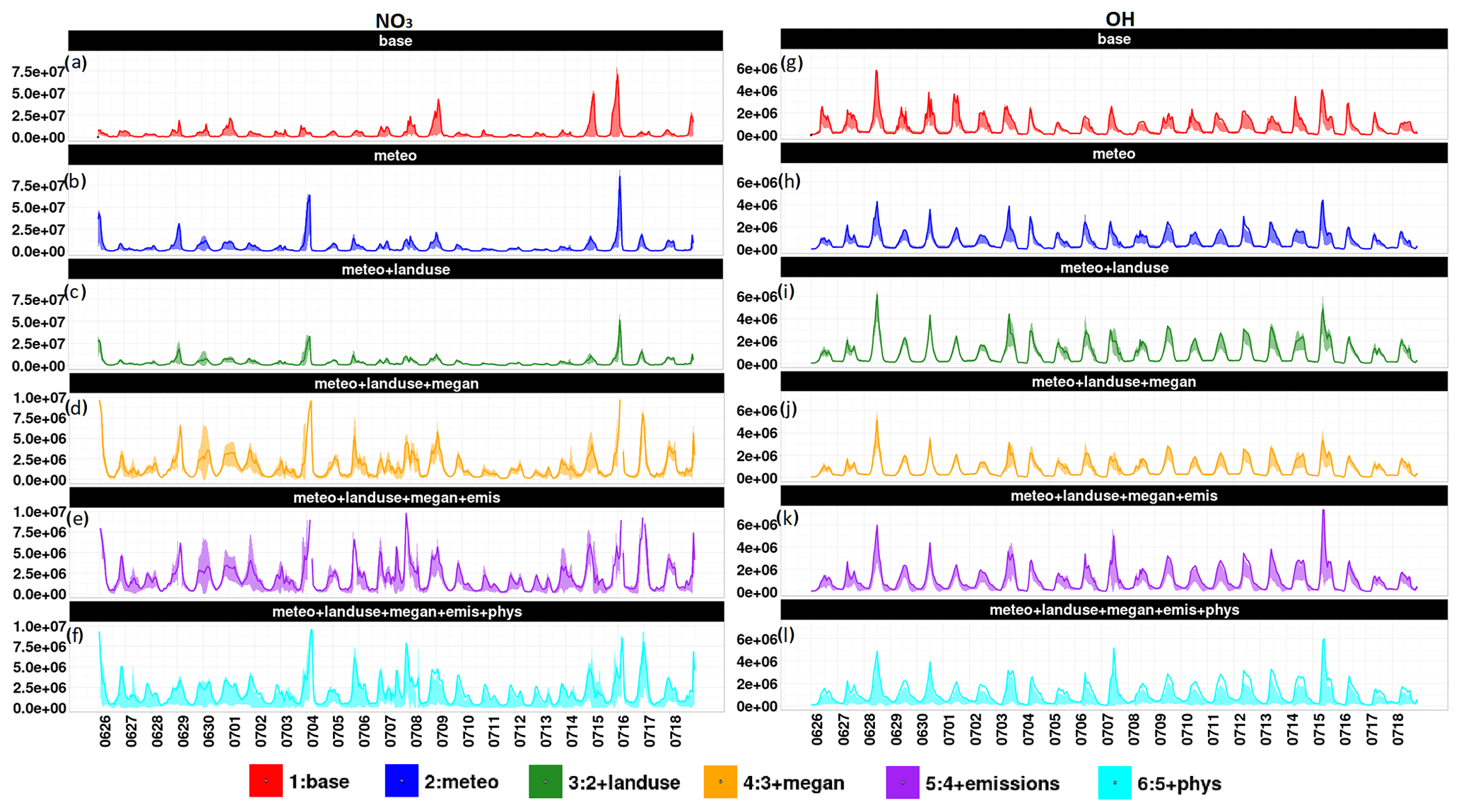
Figure 8 Time series for OH and NO₃ concentrations (both in ppb) for all of the sensitivity cases explained above. The color schemes are shown at the bottom. The name of each case is written above each time series. Note that the NO₃ columns have two different scales because of visibility issues. Both plots use the same units (molecules cm⁻³ s⁻¹), but the scale for NO₃ changes for certain test cases.

Compared to NO₃, OH concentrations remain more stable among in all sensitivity cases, changes being generally limited to several tenths of a percent. These changes are difficult to explain in the absence of a dedicated budget study, which is beyond the scope of this paper. For instance, the combined effect of land cover and BVOC emission changes is relatively small, probably because increased loss reactions with terpenes are compensated for by diminished losses with isoprene. Increases in daily maximum OH due to anthropogenic emission changes could be due to a more effective OH recycling via the NO + HO₂ reaction. When it comes to the canopy test case, the modification of swrd results in a decrease in OH concentration by a factor of 1.4 on average, while the K_z and wind speed modification does not result in any significant change in the concentration of OH. For more densely forested grid cells, the inside-canopy radiation has a higher reduction, and as a consequence the OH concentration also has a higher reduction. Since no OH concentration measurements were available from this campaign (the FAGE instrument deployed by the University of Lille having unfortunately encountered technical problems), they have been estimated from global inside-canopy radiation and a climatological (above-canopy) maximum OH concentration of 3–6×10⁶ molecules cm⁻³ (Mermet et al., 2021). Daily OH maxima estimated in this way were about a factor of 2 to 3 below our simulated inside-canopy concentrations.

4.4 Particulate species

Figure 9 shows a comparison of all performed sensitivity cases to measurements at the Salles-Bilos site for particulate species (in µg m⁻³). PM_2.5 observations during the campaign period culminate at more than 20 µg m⁻³ on 7 July. Some higher hourly values (also visible in OA) on 6 July are due to a local fire that is not further analyzed here. About half of PM_2.5 is composed of organic aerosol (10 µg m⁻³). The simulated concentrations of secondary inorganic aerosol (sulfate + nitrate + ammonium), sea salt, black carbon, and dust are about 3.0, 1.6, 0.9, and 7.6 µg m⁻³, respectively, in the model, pointing to a significant dust contribution at this time at Salles-Bilos. The base case simulations show large PM_2.5 concentrations around this date (from 6 to 9 July) at Salles-Bilos, reaching 60 µg m⁻³. This species is very sensitive to the chosen meteorology. With ECMWF meteorology, the peaks decrease to 40 µg m⁻³; however, another dust-related, yet unobserved, peak at Salles-Bilos occurs on 13 July. Both of these episodes were seen in aerosol optical depth (AOD) observations at the Arcachon AERONET station (a city on the coast to the west of Bordeaux).

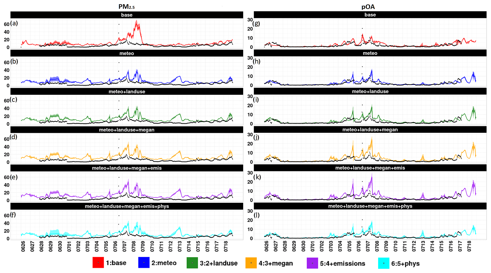
Figure 9 Time series for PM_2.5 and organic aerosols (OA) (both in µg m⁻³) for all the sensitivity cases explained above. The color schemes are shown at the bottom. The name of each case is written above each time series.

Besides dust, OA is the main driver of observed and simulated PM_2.5 variability. During the sunny, calm, and high-oxidation periods, from 4 to 7 July and then from 14 to 18 July, observed OA concentrations reach about 10 µg m⁻³. This time pattern is rather well reproduced by the base simulation; OA peaks are, however, overestimated (see below). It is concluded from the model results and known OA sources that most of this is biogenic SOA (84 % in simulations at Salles-Bilos over the campaign period). For instance, the concentration of anthropogenic (primary and secondary) OA is quite low at this site (with an average of 0.11 µg m⁻³ over all test cases).

Average OA concentrations (Fig. 9) are mostly impacted by the biogenic emissions sensitivity case (+26 %), the canopy test case (−24 %), the land cover changes (+22 %), and the meteorological test case (−7 %). The test case that has the least effect on the concentration of OA is the anthropogenic emission test (+3 %). Changing the biogenic emissions causes a significant increase in the concentrations of terpenoids (sum of monoterpenes and sesquiterpenes), which then increases the formation of biogenic OA. The land cover changes also impact the concentration of OA for the same reason. Changing the K_z parametrization and inside-canopy radiation decreases OA, BSOA, and the concentrations of the three oxidants (OH, NO₃, and O₃) that participate in the biogenic OA formation process, while increasing the concentrations of terpenes (its major precursors). Thus, a lesser portion of the emitted terpene is oxidized and less BSOA is therefore formed.

The final test case shows enhanced OA concentrations with respect to the base case, and an additional difference lies in the chemistry behind the production of OA, as will be discussed in Sect. 4.5. In the final test case the concentrations of precursors and radicals correspond better to observed data, as shown in Sects. 4.1 and 4.3. The remaining overestimation could be due to the already stated oxidant overestimation for O₃ and NO₃ (noting that OH cannot be verified). It could also be due to the scheme used for the simulation of OA; thus, forthcoming work should test the sensitivity due to different aerosol schemes.

4.5 BSOA formation from different precursors and oxidant pathways

As pointed out in the Introduction, different precursor and oxidant pathways for BSOA buildup have been found in the literature (e.g., Hallquist et al., 2009; Xu et al., 2015; Qin et al., 2018) for different types of forest, and it is interesting to address this question for a maritime pine forest. To do so, two sets of additional simulations have been performed for the base case and the final case, in which the formation of BSOA from each precursor and via each oxidant was followed individually during the model run. These results are presented in Figs. 11 and 12.

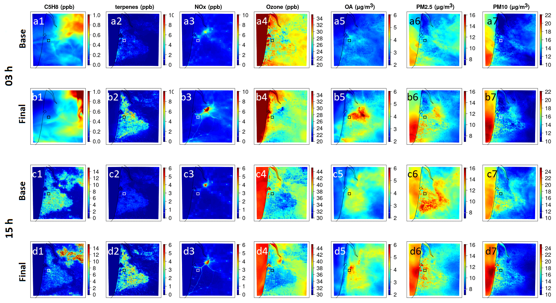
Figure 10 Average concentrations over the campaign period for species of importance for this study (compound names and associated units are written above each column) for 03:00 (first two rows) and 15:00 LT (second two rows) for the base simulation (first and third rows) and final simulation (second and fourth rows). Note that the scales are different for each plot. The measurement site at Salles-Bilos is located in the middle of the white or black rectangle in each plot.

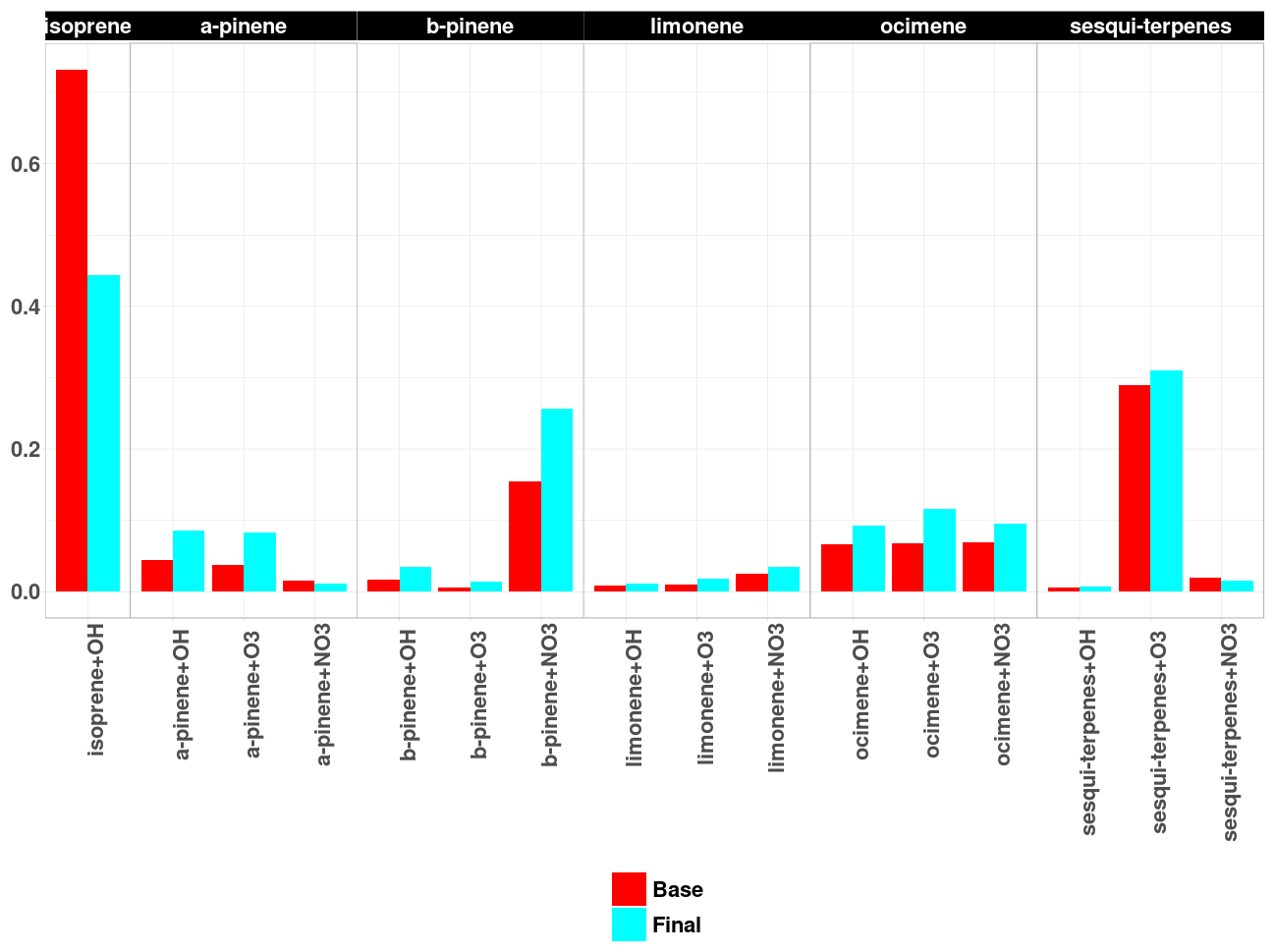
Figure 11 Bar plots showing the formation of BSOA averaged over the campaign period (in µg m⁻³) from all precursors and oxidants. The colors of the bars indicate which simulation they are from. The reactions are shown on the x axis.

For the base case scenario, the formation of BSOA is mostly achieved from isoprene oxidation by OH. After the corrections made for the land cover, the tree types, and the physical parameters (introduced in Sect. 3.6), in the final test case isoprene + OH stays the most important BSOA formation pathway, but monoterpenes become the dominant precursor group. The attack on β-pinene by NO₃ is noteworthy in this group, in accordance with results found, for example, as part of the 2013 SOAS study in the southeastern US (Xu et al., 2015). The reaction of sesquiterpenes with O₃ is a third important reaction pathway.

Figure 12 Daily averaged concentrations of BSOA per precursor and per oxidant (in µg m⁻³). The colors for each reaction are defined in the legend. The base case simulation results are shown in (a), while the final case results are shown in (b).

Looking at which oxidant is responsible for BSOA formation, the majority of BSOA in the base test case is formed from OH radical reactions (by about half, i.e., 47 %), followed by O₃ (nearly 30 %) and NO₃ (more than 20 %). In the final test case, the BSOA formation becomes more evenly distributed between the three precursors: OH stays in majority (by 36 %), while the other two oxidants follow closely (33 % for NO₃ and 31 % for O₃). These results can be compared to those reported by the BVOC reactivity study at Salles-Bilos (Mermet et al., 2021) based on measured BVOC species and O₃, OH, and NO₃ estimated from chemical equilibrium and solar radiation, even if this work addresses different features. In this study, the β-caryophyllene + O₃ reaction makes by far the largest contribution to BVOC reactivity. In our simulations, β-caryophyllene is part of the sesquiterpene species family, which still makes an important contribution. Also, monoterpenes strongly contribute to BVOC reactivity, while isoprene is only a minor contributor. In general, O₃ is the major oxidant, followed by OH, while NO₃ only makes small contributions. Differences with respect to the experimental study (Mermet et al., 2021) to our study can be explained by many factors that we do not attempt to quantify here. For example, (i) the experimental study considers local oxidation rates, and those within the canopy are used here, while our study considers contributions within air masses arriving at the receptor site; (ii) our study overestimates nighttime O₃, which leads to high NO₃ radical formation (see Fig. 8) and could explain the larger share of NO₃ oxidation pathways; (iii) in the experimental study estimated OH is smaller than that in our study (see Sect. 4.3); and (iv) the initial share of BVOC species might be different even if Fig. 7 shows broad agreement for major BVOC species in the final case.

Interesting insight can also be obtained from analyzing the daily averaged concentrations of BSOA being formed from the different reaction pathways of BVOCs with oxidants presented in Figs. 11 and 12. While the concentration of total BSOA stays quite similar between the two simulations (with the exception of some days, especially 7 July), the chemistry behind their formation changes significantly. The contribution of isoprene in the formation of BSOA becomes lower in the final case, while the contributions of the β-pinene + NO₃ pathway and the oxidation of other terpenes increase significantly. Figure 12 shows that this is especially true for 7 July when simulated BSOA was most overestimated. As terpene levels were well simulated on this day, this could most probably be due to an overestimation of radical concentrations (NO₃ and OH) and/or SOA yields. However, as many different pathways contribute to BSOA, it is difficult to pinpoint a specific one that is responsible for this BSOA overestimation.

5 Spatial distribution of BSOA, precursors, and oxidants over the Landes forest

5.1 Average spatial distribution during the LANDEX campaign

After this first analysis of time series at the measurement site where intensive campaign data were available, we now would like to extend the discussion to a broader spatial scale, covering the Landes forest and its surroundings. To achieve this, we first present near-surface 2D maps (of the high-resolution domain covering the Landes forest) of specific species pertaining to our study averaged over the campaign period (between 26 June and 20 July 2017). The interest here is to analyze how the changes in the model from the baseline test case to an updated local or regional configuration modify the concentrations seen in these 2D fields.

Due to the short lifetime of terpenes during daytime (a few hours in most cases), the area of enhanced total terpene concentrations (at 15:00 LT) closely corresponds to the high-emission zone of the Landes forest. In the high-resolution simulation (1 km) with the canopy parametrization and all other local databases, average terpene concentrations are heterogeneous, varying from several parts per billion to up to 10 ppb. During the night (03:00 LT), terpene levels are at their maximum near the northeast edge of the forest. This is due to larger emissions there (Fig. 4c) and lower O₃ concentrations leading to diminished loss (Fig. 10). The higher concentration of O₃ observed over the ocean in Fig. 10a4–d4 is because of the lower deposition of O₃ over bodies of water, since its dry-deposition speed is lower.

As expected, a strong increase is seen in the final case compared to the base case test over the whole domain. This is mainly due to enhanced terpene emissions in the local databases.

Isoprene concentrations in the final case simulation are also enhanced over the Landes forest; they are higher over forested areas to the northeast of Bordeaux that include more isoprene-emitting species like oaks.

The NO_x 2D fields display the largest concentration levels in the urban Bordeaux area, and these are even larger at night due to enhanced vertical stability. In the simulation using a high-resolution emission inventory, highways starting from Bordeaux are displayed, such as weak plumes in the surroundings of the city. It is also interesting to compare the difference in resolution between the base and final simulations, noticeable in the 2D images shown in Fig. 10a3–d3. Daytime NO_x concentrations in the Landes forest are relatively low (typically 2–3 ppb). According to this, photochemical O₃ production is not very active over the Landes forest, since daytime O₃ levels are lower there (35–45 ppb) than in surrounding areas (45–55 ppb), mainly due to loss by reactions with terpenes or by dry deposition, with the exception of an O₃ plume to the southwest of Bordeaux. Nighttime O₃ shows local minima in the surroundings of the metropole, below 20 ppb, due to NO titration. If the results seen in Salles-Bilos can be extrapolated to the whole Landes forest, then simulated nighttime O₃ levels are likely to be overestimated. Maximum values of NO_x do not change between the base case and final simulations; however, their spatial precision improves because of the increase in the resolution of the emissions inventory from the emission test case onwards.

Nighttime OA in the updated configuration shows a hot spot at the northeastern edge of the Landes forest, corresponding to regions with enhanced terpene concentration levels. This effect is not seen in the baseline simulations, where concentrations are higher in the center of the forest (Fig. 10). The nighttime concentrations for the base case simulations are also lower. Daytime OA is generally enhanced over the Landes forest, showing that large terpene emissions there lead to local OA buildup. In this averaged field, no BSOA export from the Landes forest can be distinguished. Maximal concentrations occur within the forest at about 25 km from the coastline. It is hypothesized that this is related to a sea breeze front forming along the Atlantic shoreline. This is also suggested by the temperature fields at 15:00 LT (not shown), which show large gradients (nearly 10 K) between the coast and about 20 km inland. This phenomenon will be addressed in more detail in the next section. This sea breeze is also seen in the baseline simulations when looking at hour-by-hour changes in OA concentration. In the base case simulations concentrations are lower during daytime as well (similar to what was seen at nighttime).

It can be noted that simulated BSOA concentrations alone are above the WHO target of 5 µg m⁻³ for PM_2.5, even if they are expected to be lower during other seasons (however, we have already shown that they are overestimated with respect to measurements at the Salles-Bilos site). The spatial structure of the PM_2.5 and PM₁₀ simulations broadly follows that of BSOA simulations with a major exception over the sea, where sea salt makes an additional contribution to PM₁₀.

The concentrations of the base sensitivity test and the final sensitivity case were compared to regional air quality station measurements discussed in Sect. 2 (Fig. 13). These comparisons (Fig. 13a) show that the bias (simulation–observation) for NO₂ for all stations (regardless of the type of station) for the final test drops to −1.4 ppb (from an initial −2.9 ppb for the base simulation), while the averaged correlation coefficient gets to 0.42 in the final test from 0.37 for the base case. NO_x concentrations show a bias (simulation–observation) and correlation coefficient of −2.4 ppb and 0.57, respectively, in the final test case compared to −3.1 ppb and 0.51 in the base simulation, respectively (Fig. 13b). Unfortunately, the concentrations of O₃ (while being measured) at the air quality stations were not available for comparison for the period of the simulations.

Figure 13c and d also illustrate the comparisons of PM_2.5 and PM₁₀ at air quality stations of the ATMO-NA network. It is interesting to notice that the profiles seen at all stations are quite similar to each other. For PM₁₀, the results show an average correlation coefficient of 0.3 and 0.42 and an average bias (simulation–observation) of −3.3 and −2.9 µg m⁻³ for PM₁₀ for the base and the final sensitivity test, respectively. For PM_2.5 in the base and the final sensitivity test, a correlation coefficient of 0.4 and 0.58 and a bias (simulation–observation) of +4.8 and +4.1 µg m⁻³ are seen, respectively. Apparently refining the simulations through the sensitivity tests adds physical information, as can be seen when looking at the improved correlation coefficients (for PM and NO_x).

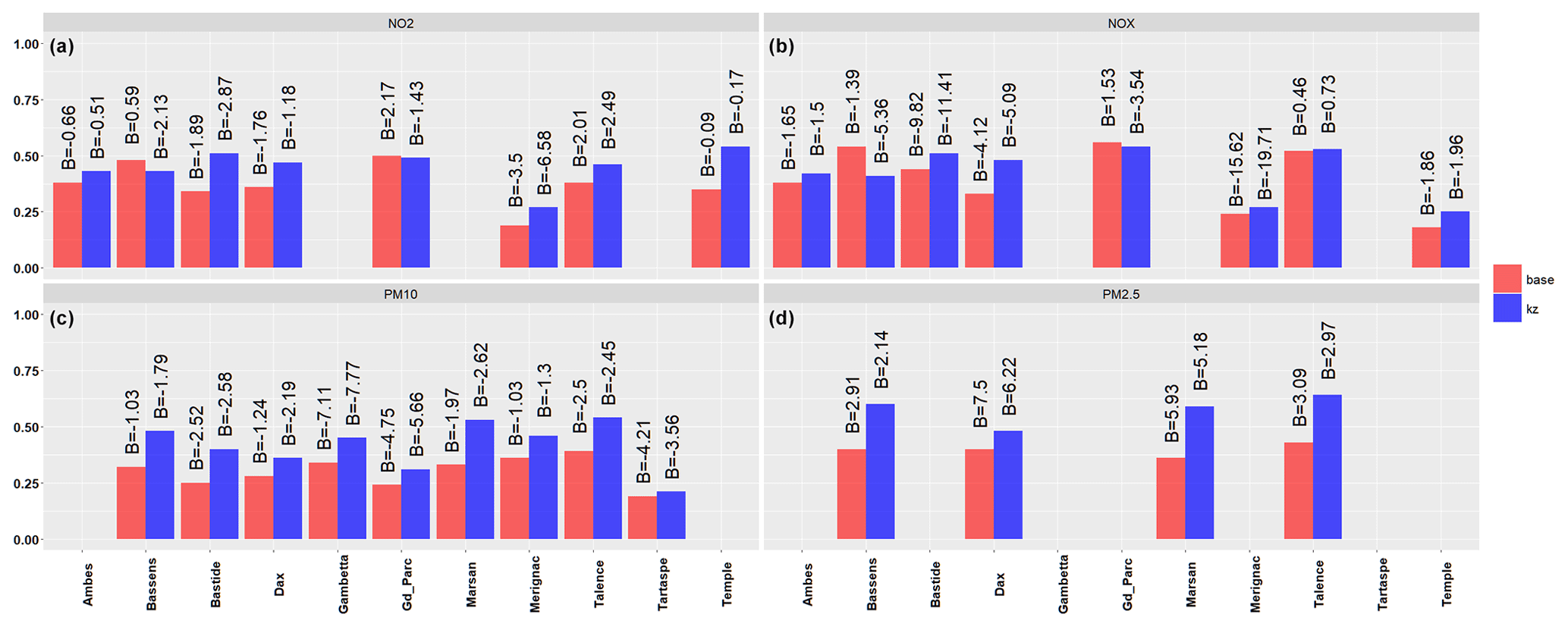
Figure 13 Statistics for the comparisons of measurements performed at air quality stations for NO₂, NO_x, PM₁₀, and PM_2.5 in the simulations. The y axis shows the correlation coefficient, while the bias (simulation–observation) for each station is written on each bar. The comparisons involve the base case (in red) and the final test case (in blue).

5.2 A case study for the impact of sea breeze fronts

In the previous section, mention was made of the crest of the high afternoon BSOA levels within the Landes forest about 25 km from the coastline, with the proposed hypothesis of a potential sea breeze front forming along the Atlantic coastline. Indeed, Planchon and Cautenet (1997) note that sea breeze fronts can go up to 40 km inland from the French Atlantic coast, and other references show similar values (i.e., Lerczak et al., 2001), while Hughes and Veron (2018) show a maximum of 200 km inland movement in specific situations. In this section, we wish to address this feature using a case study during the low wind period from 5 to 7 July, which should be prone to the development of sea breeze systems. Figure 14 shows the time evolution of BSOA (Fig. 14a1–a6 for 5 July and Fig. 14d1–d5 for 7 July) during both 5 and 7 July (a link to an animation is accessible in Sect. S7). This shows a tendency for BSOA to be transported to the coast by easterly winds during nighttime (shown only in animations). Then the development of a sea breeze front approximately starting at noon and progressing over the land during the afternoon can be seen. This front is materialized by pronounced gradients in temperature (warmer on the landward side, Fig.14b1–b6, e1–e5) and a ridge of high BSOA in the vicinity of the front. Wind fields depict this sea breeze system well (Fig. 14c1–c6, f1–f6). These figures dramatically show that, in addition to chemical BSOA formation, such transport processes are major drivers for the BSOA variability over the Landes forest; this is visible, for example, by comparing pictures of 11:00 and 14:00 LT on 5 July.

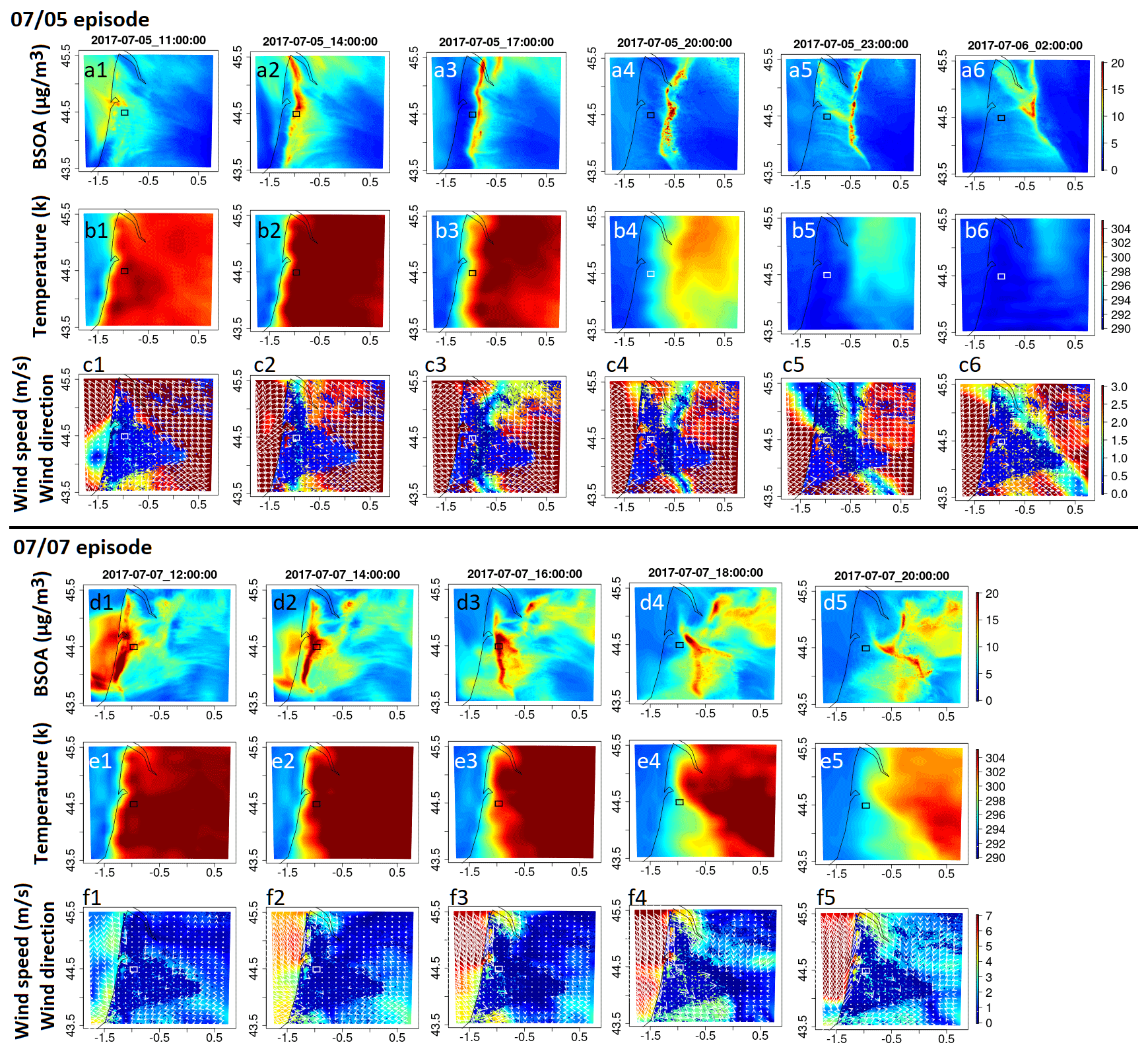
Figure 14 Sea breeze event for 5 and 7 July. The date and time of each panel are shown at the top of each panel, and each row represents one variable or species, with the name and the unity mentioned on the y axis.

This phenomenon also affects the species time series at the Salles-Bilos site and needs to be taken into account to interpret the LANDEX campaign data, in addition to the general synoptic situation and local dispersion conditions upon which previous studies have already focused (Kammer et al., 2018; Bsaibes et al., 2020; Mermet et al., 2021). Figure 15 shows the passage of the sea breeze front at Salles-Bilos as a concomitant sharp decrease in BSOA and temperature during afternoon hours. Differences in the exact timing of the frontal passages are especially visible for 7 July, when observed organic aerosol concentration at the Salles-Bilos site drops earlier than the simulated one. This could be due to other factors, e.g., an increase in boundary layer height not accounted for in the simulations.

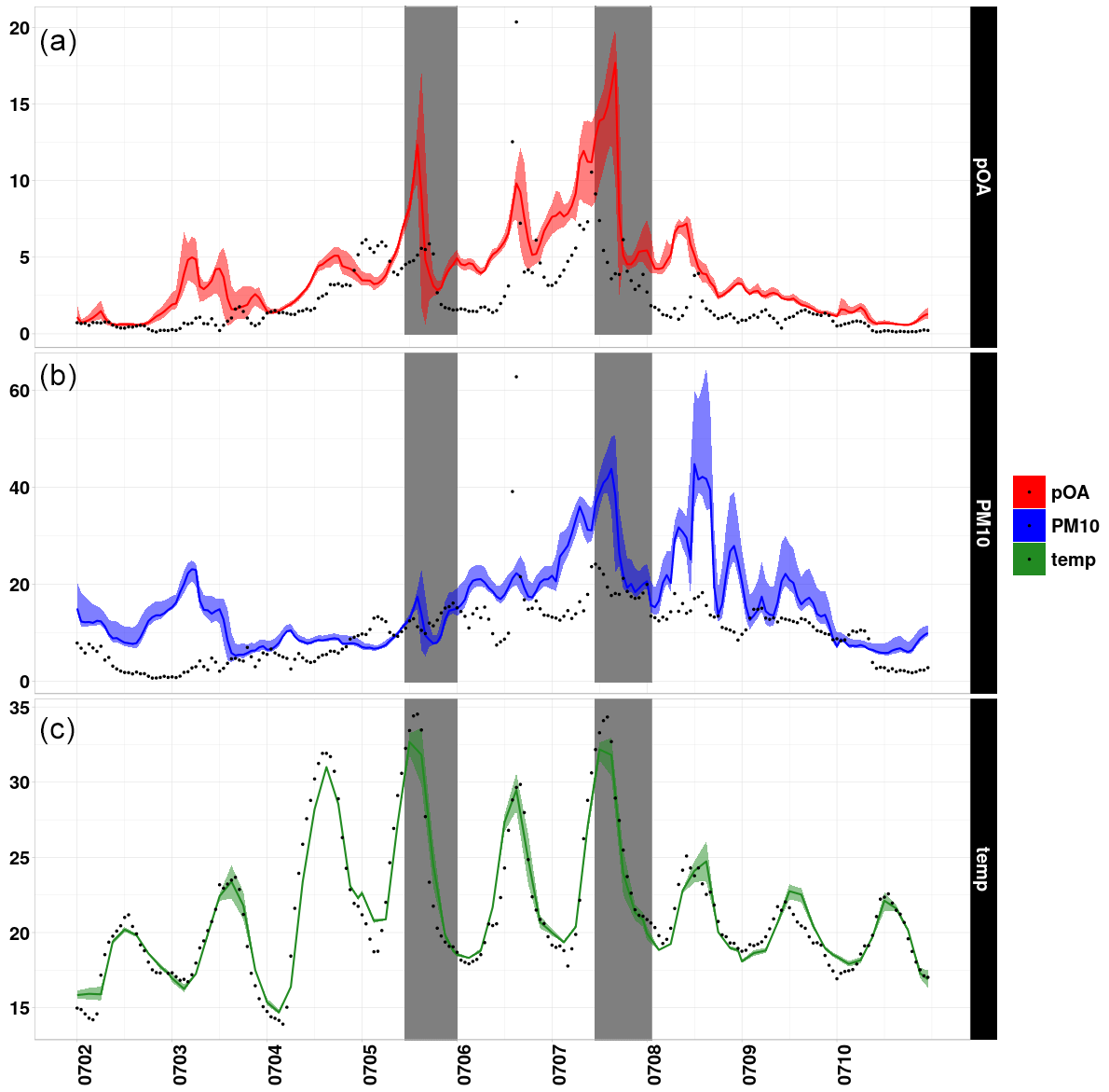
Figure 15 Time series for BSOA (µg m⁻³), PM₁₀ (µg m⁻³), and temperature (k) for the two sea breeze episodes compared to measurements. The episodes are highlighted in each panel. The confidence interval corresponds to the concentrations seen in a 11 km × 11 km square around the measurement site. The gray zones correspond to times of the passage of the sea breeze front.

6 Conclusions

This work aims to study the formation of BSOA in a forest canopy using the CHIMERE chemistry transport model. For this purpose, we have examined the Landes forest, one of the largest pine forests in Europe, located in southwestern France. The forest is populated by a 95 % majority of maritime pines, a monoterpene- and sesquiterpene-emitting tree species. It is also a region with rather homogeneous land cover and weak anthropogenic influences. The measurements used in this study were performed during the LANDEX episode 1 field campaign, carried out in the summer of 2017 with the goal of understanding the atmospheric chemistry related to biosphere–atmosphere interactions. At the Salles-Bilos site within the Landes forest, a set of detailed in situ measurements has been obtained to illustrate these features.

In order to study the formation of BSOA we had to first focus on the entire physicochemical system inside the forest canopy. Therefore, we performed multiple test cases updating the representation of the forest in the chemistry transport model. It has to be kept in mind that while the goal is partially improving the performance of the model for this specific region, the sensitivity cases are also meant to show the effects of changing inputs or the simulation of different physical parameters on the concentration of different atmospheric species. Since the CHIMERE chemistry transport model does not include an online canopy model, we have tried to mimic the simulation of a forest canopy by adding region-specific parametrizations.

The modeling chain consists of three nested domains, one covering the entirety of Europe, the intermediate domain focused on France, and the final nested domain focused entirely on the Landes forest with a horizontal resolution of 1 km. In total, six sensitivity cases were performed, focusing on measuring meteorological input fields and land cover inputs; improving the biogenic emission factors by correcting the type of trees present for this region in the MEGAN model; discerning anthropogenic emissions; and finally adding a parametrization prepared specifically for the Landes forest for the simulation of vertical diffusivity, wind speed, and penetration of radiation inside the forest canopy.

Each of the studied scenarios shows effects on different species; for example, not surprisingly NO_x is quite sensitive to changes in anthropogenic emission inputs, while terpenes show a double sensitivity to changing the emission factors or changing the vertical diffusivity and wind speed in the area. What has been noted is that the physical test case (taking into account physical changes in the simulations of vertical diffusivity, wind speed, and radiation penetration inside the canopy) presents a closer representation of the measurements observed at the Salles-Bilos site, as well as of several air quality measurement stations around the forest. Using the final test case and the base test case, we also simulated the formation of BSOA from different precursors and oxidants. This showed us that the formation of BSOA for the base case scenario comes from the wrong precursors, as BSOA is mostly formed from the oxidation of isoprene, which is not accurate for this region. The formation of BSOA changes to terpenes (specifically sesquiterpenes and β-pinene) in the final simulations, which is more in line with the observations in the Landes forest. These final results are more in line with what is seen in the measurements for the Landes forest as well.

We also make evident spatial gradients between the forest and the surrounding areas, especially for BSOA and short-lived species like terpenoids and isoprene. The formation of BSOA is quite localized inside the forest, consistent with high BVOC reactivity (which leads to BSOA formation in one step in our model, meaning that in reality BSOA formation could take some more time as a multi-step process). We also evaluated our simulations at a regional scale, which showed an improvement for all species measured at almost all air quality stations located around the forested area. Still, for PM_2.5 the positive bias (simulation–observation) subsides, probably due to the positive bias in OA, a major contributor to PM_2.5 concentration.

In addition, we analyzed the impact of transport processes within the forest area and focused on sea breeze effects. We found for a period with low winds, sunny conditions, and enhanced BSOA buildup that the sea breeze front passes over the Salles-Bilos measurement site and advects cleaner marine air masses. This manifests as a steep decline in temperature and BSOA at the Salles-Bilos measurements site during afternoon. Thus, advection is important to consider in addition to chemistry for understanding the observed time series well, even for a measurement site carefully chosen in an environment with a rather homogeneous land cover.

What we have tried to point out here is the necessity of a coupled canopy model or a sub-grid simulation scheme when it comes to simulating areas with a particular physical representation like a forest. This type of sub-grid information exists for urban areas or for deserts, but our results show that it is also important to investigate it for forested areas in chemistry transport models. The next steps for this study are to investigate the reasons for the overestimation of the minima concentrations of O₃ inside the forest and the overestimation of the BSOA (for some peaks) even after modifications are made. It is also important to understand the (still) overestimated concentrations of isoprene in the simulations, even after modifications to the tree types and land cover in the area. Further studies should also include the usage of different SOA simulation schemes in order to test their sensitivity to precursor or oxidant changes and the simulated concentrations of BSOA. It would be interesting to test the physical parametrization used in this study on other forests to see how the parametrization would perform elsewhere. Another interesting continuation of this work would be making hypotheses about the future of the forest: what effects would climate change modifying the land cover and potentially causing longer periods of drought have on a pine forest and its atmospheric chemistry? This question has become of even greater importance due to the sad reality of massive forest destruction caused by the July 2022 fires.