Estimating enhancement ratios of nitrogen dioxide, carbon monoxide and carbon dioxide using satellite observations

Using co-located space-based measurements of carbon dioxide (CO₂) from the Orbiting Carbon Observatory-2 and Orbiting Carbon Observatory-3 (OCO-2/3) and carbon monoxide (CO) and nitrogen dioxide (NO₂) from the TROPOspheric Monitoring Instrument (TROPOMI), we calculate total column enhancements for observations influenced by anthropogenic emissions from urban regions relative to clean background values. We apply this method to observations taken over or downwind of 27 large (population of >1 million) urban areas from around the world. Enhancement ratios between species are calculated and compared to emissions ratios derived from four globally gridded anthropogenic emissions inventories. We find that these global inventories underestimate CO emissions in many North American and European cities relative to our observed enhancement ratios, while smaller differences were found for NO₂ emissions. We further demonstrate that the calculation and intercomparison of enhancement ratios of multiple tracers can help to identify the underlying biases leading to disagreement between observations and inventories. Additionally, we use high-resolution CO₂ inventories for two cities (Los Angeles and Indianapolis) to estimate emissions of CO and NO₂ using our calculated enhancement ratios and find good agreement with both a previous modelling study for the megacity of Los Angeles and California Air Resources Board (CARB) inventory estimates.

1 Introduction

Improving air quality and reducing greenhouse gas emissions are focuses of environmental policy from global to municipal levels (Gurney et al., 2018a). Emissions inventories provide information about the distribution and sources of air pollution and greenhouse gas emissions as well as their trends over time. These inventories are constructed using bottom-up approaches: information on socio-economic activity is used alongside expected emissions factors for these activities to model emissions (Gurney et al., 2012; Janssens-Maenhout et al., 2019). Atmospheric measurements have been shown to be useful as part of top-down approaches in validating and refining these emissions inventories (McKain et al., 2012; Duren and Miller, 2012).

The expansion of the constellation of Earth-observing satellites taking measurements of greenhouse gases and air pollutants has led to observations over urban regions with unprecedented spatiotemporal coverage. Kort et al. (2012) used observations from the Greenhouse Gases Observing Satellite (GOSAT), launched in January 2009, to measure enhancements of atmospheric carbon dioxide (CO₂) over megacities. Since the launch of the Orbiting Carbon Observatory-2 (OCO-2) in July 2014 (Crisp et al., 2004), further studies have characterized emissions from urban regions (e.g., Wu et al., 2018; Reuter et al., 2019). The Orbiting Carbon Observatory-3 (OCO-3) aboard the International Space Station (ISS) since May 2019 (Eldering et al., 2019) has provided additional observations of CO₂ in urban areas (Kiel et al., 2021). Satellite remote sensing of additional air pollutants has been greatly expanded with the launch of the TROPOspheric Monitoring Instrument (TROPOMI) aboard the Sentinel-5 Precursor (S5P) satellite on 13 October 2017 (Veefkind et al., 2012). Early investigations into the TROPOMI carbon monoxide (CO) and nitrogen dioxide (NO₂) products have shown the ability of TROPOMI to map concentrations of these air pollutants at the city scale (e.g., Borsdorff et al., 2018; Zhao et al., 2020).

Enhancement ratios have been shown to be useful in evaluating the validity of emissions inventories and estimating emissions from a variety of anthropogenic sources of greenhouse gases and air pollutants. Wunch et al. (2009) used a ground-based remote sensing instrument to measure the diurnal variation in greenhouse gases within California’s South Coast Air Basin (SoCAB) and calculate enhancement ratios between CO₂, CO, CH₄ and N₂O. Hedelius et al. (2018) used a combination of ground-based and satellite-based remote sensing instruments and a Lagrangian particle dispersion model to derive improved enhancement and emissions ratios between CO₂, CO and CH₄ for the SoCAB while also demonstrating good agreement between ratios computed using different methods. Enhancement ratio methods involving both greenhouse gases (primarily CO₂) and air pollutants have also been used to investigate the combustion characteristics of anthropogenic activities; Silva and Arellano (2017) used satellite measurements of CO₂, NO₂ and CO to show a correlation between the dominant forms of combustion and both NO₂ : CO and CO : CO₂ enhancement ratios in 14 regions from around the world. More recently, Lama et al. (2020) used measurements from TROPOMI to investigate burning efficiencies in six megacities by computing NO₂ : CO enhancement ratios and comparing to emissions ratios from global inventories. Plant et al. (2022a) used TROPOMI methane and CO enhancements to assess methane emissions from several US cities.

In this paper, we describe a method to compute enhancement ratios between CO₂, CO and NO₂ over 27 large urban areas by combining measurements from three different space-based instruments. We use measurements of atmospheric CO₂ from OCO-2 and OCO-3 and measurements of CO and NO₂ from TROPOMI to measure anomalies over urban areas relative to a regional background. Results across multiple overpasses of these urban regions are used to derive enhancement ratios, which are then compared to ratios calculated from four global emissions inventories: the Emissions Database for Global Atmospheric Research (EDGAR), the Open-source Data Inventory for Anthropogenic CO₂ (ODIAC), the Fossil Fuel Data Assimilation System (FFDAS), and the Mapping Atmospheric Chemistry and Climate and CityZen (MACCity) inventory.

In Sect. 2, we will describe the datasets and global emissions inventories used in our analyses. In Sect. 3, we will describe our approach to derive enhancement ratios between gases from satellite measurements. Section 4 will present the results of this analysis, and Sect. 5 will discuss the implications of these findings. Finally, Sect. 6 will summarize our conclusions and suggest future work.

2 Data

2.1 OCO-2

We use measurements of the column-averaged dry-air mole fraction of carbon dioxide ($X_{{\mathrm{CO}}_{\mathrm{2}}}$) from OCO-2 (Crisp et al., 2004). OCO-2 was launched on 2 July 2014 into a Sun-synchronous orbit with an Equator crossing time of about 13:30 (ascending node) as part of the afternoon constellation (or A-train constellation) of satellites. OCO-2 has been collecting science measurements of $X_{{\mathrm{CO}}_{\mathrm{2}}}$ since 6 September 2014, collecting around 1 million total column observations per day (Crisp et al., 2017). The OCO-2 instrument includes three different grating spectrometers that measure reflected solar radiation in the near-infrared (NIR) and shortwave infrared (SWIR) spectral regions. The spectral bands include the O₂ A band from 0.7576–0.7726 µm, along with the “weak” and “strong” CO₂ bands measured at 1.5906–1.6218 and 2.0431–2.0834 µm, respectively. Measurements are taken in a horizontal row with eight cross-track footprints, with three rows of observations collected every second. Each individual footprint has dimensions of approximately 2.25 km in the along-track direction and up to 1.29 km in the cross-track direction (depending on the satellite orientation). OCO-2 observes in three different modes of operation. In nadir mode, the observations are taken at the sub-satellite point and measurements taken over water are typically filtered out. In glint mode, the satellite makes observations near the point of Earth's surface where sunlight is specularly reflected (Crisp et al., 2017; Eldering et al., 2019). Finally, OCO-2 can operate in target mode, where a small area of Earth is observed for several minutes while the satellite passes overhead. This mode is often used for the validation of measurements against ground-based remote sensing stations (e.g., Wunch et al., 2017).

For this study we use bias-corrected measurements of $X_{{\mathrm{CO}}_{\mathrm{2}}}$ from the OCO-2 Lite level 2 version 9 (Kiel et al., 2019) files accessed from the Goddard Earth Sciences Data and Information Services Center (GES DISC) (https://disc.gsfc.nasa.gov/, last access: 8 February 2020). The bias-correction process for OCO-2 adjusts $X_{{\mathrm{CO}}_{\mathrm{2}}}$ based on spurious correlations with retrieved aerosols, surface albedo, and the difference between the vertical gradients of the retrieved and a priori CO₂ profiles. Version 9 includes an additional surface-pressure-based bias correction to account for pointing offsets which can cause greater uncertainties in regions with considerable topographic changes. Binary quality flags are provided in the files to indicate high- and low-accuracy measurements; for this study we only use measurements that have been flagged as “good”.

2.2 OCO-3

We also use measurements of $X_{{\mathrm{CO}}_{\mathrm{2}}}$ from OCO-3 aboard the International Space Station (ISS). OCO-3 was launched to the ISS on 4 May 2019 and began providing science measurements on 6 August 2019. The OCO-3 instrument is a spectrometer nearly identical to OCO-2, measuring spectra in the O₂ A band and weak and strong CO₂ bands to provide an eight-footprint swath of parallelogram-shaped soundings measuring approximately 1.6 km in the cross-track direction by 2.2 km in the along-track direction, with three rows of observations taken every second (Eldering et al., 2019). OCO-2 pointing is carried out by manoeuvers to the spacecraft, which is not possible on the ISS; thus OCO-3 is equipped with a pointing mirror assembly (PMA). In addition to the three observation modes described for OCO-2, the PMA enables OCO-3 to scan in an additional “Snapshot Area Map” (SAM) mode, where a two-dimensional area is swept out by adjacent swaths of measurements. This mode measures across regions on the order of 100 km × 100 km, with the goal of capturing detailed maps of sources of CO₂ such as cities, fossil-fuel-burning power plants and volcanoes. According to the OCO-3 SAM web page (https://ocov3.jpl.nasa.gov/sams/index.php, last access: 10 March 2023), between 6 August 2019 and 30 June 2020 there were over 2000 SAM manoeuvers executed by OCO-3, with around half of these instances corresponding to sites influenced by anthropogenic sources of CO₂.

Bias-corrected measurements of $X_{{\mathrm{CO}}_{\mathrm{2}}}$ from the early (VEarly) release of the OCO-3 Lite version 10 files were accessed from the NASA GES DISC. We found that most instances of dense measurements over cities were obtained while the instrument was operating in SAM mode (Eldering et al., 2019).

2.3 TROPOMI

In our analysis, we use measurements of NO₂ and CO retrieved from TROPOMI observations. TROPOMI was launched on board the European Space Agency (ESA) Sentinel-5 Precursor (S5P) satellite on 13 October 2017 into a Sun-synchronous orbit with an Equator crossing time of about 13:30 (ascending node) and has been providing science measurements since 30 April 2018. TROPOMI is a nadir-viewing grating spectrometer that measures Earth-reflected solar irradiance in three spectral bands: in the ultra-violet and visible light (UV–Vis) band from 0.27–0.5 µm, an NIR band from 0.675–0.775 µm, and an SWIR band from 2.305–2.385 µm (Veefkind et al., 2012). Measurements in these bands enable quantification of CO and NO₂, as well as methane (CH₄; Hu et al., 2016), sulfur dioxide (SO₂; Theys et al., 2017), formaldehyde (HCHO; De Smedt et al., 2018), ozone (O₃; ESA, 2022) and additional aerosol properties. The 2600 km wide swath of TROPOMI allows for global coverage every day (van Geffen et al., 2020) (before loss of data due to clouds).

2.3.1 TROPOMI CO

A subset of TROPOMI measurements from the SWIR band (2.315–2.338 µm) are used to infer the total column of CO, along with corresponding column averaging kernels and error estimates under clear-sky conditions (Landgraf et al., 2016). From 30 April 2018 until 6 August 2019, TROPOMI CO pixels were 7 km × 7 km, with 215 cross-track pixels. From 6 August 2019 onward, the along-track resolution of the instrument was improved to 5.5 km. The TROPOMI data that we use are version 1 of the data product.

TROPOMI total column CO values exhibit a stripe bias between adjacent rows of along-track observations (Borsdorff et al., 2018). In addition to creating offsets to adjacent observations, the magnitude of the bias can change in the along-track direction. To remove this bias we use the Fourier filter destriping (FFD) method described by Borsdorff et al. (2019) as a non-uniformity correction. This algorithm involves taking the two-dimensional Fourier transform (FT) of the CO measurements from a single orbit and filtering out modes with high frequency in the cross-track direction and low frequency in the along-track direction. We identified a similar bias in the surface level values of the CO column averaging kernels, so FFD was applied to these values as well.

The quality of the measurements of the total column of CO from TROPOMI is denoted by a quality assurance value (“qa_value”) provided with each observation, with 0 indicating the lowest quality and 1 indicating the highest. Following the product user manual (https://sentinels.copernicus.eu/documents/247904/0/Sentinel-5P-Level-2-Product-User-Manual-Carbon-Monoxide/dc93c3ae-6c77-4673-8fe7-459635aba4a3, last access: 10 March 2023), we use measurements with a qa_value of 0.7 or greater, which indicates clear-sky conditions. Furthermore, we filter out measurements taken either entirely or partially over water. Finally, we convert the provided total column in moles per square metre to total column dry-air mole fractions (X_CO) in parts per billion as described in Wunch et al. (2016) using the retrieved total column of water and the provided surface pressure for each observation.

2.3.2 TROPOMI NO₂

Observations over 0.405–0.465 µm from the UV–Vis spectrometer in TROPOMI are used to infer the tropospheric vertical column densities of NO₂ (van Geffen et al., 2020). The TROPOMI NO₂ ground sampling distance is approximately 3.5 km in the cross-track direction, with the same along-track distance as the CO product. Similar to the TROPOMI CO product, the quality of measurements of the tropospheric column of NO₂ is described by a qa_value field. Following the NO₂ product user manual (https://sentinels.copernicus.eu/documents/247904/4682535/Sentinel-5P-Level-2-Product-User-Manual-Nitrogen-Dioxide/ad25ea4c-3a9a-3067-0d1c-aaa56eb1746b, last access: 10 March 2023), we use only NO₂ measurements with a qa_value of 0.75 or greater. No stripe bias correction is needed for the NO₂ product, as corrections have already been applied to the values provided in the NO₂ level 2 files. Again the column densities are converted to dry-air mole fractions using the retrieved column of water and reported surface pressure. Finally, tropospheric averaging kernels are derived from the provided total column averaging kernels following the method described by Eskes et al. (2019).

2.4 Cities

For information on the location and extent of cities from around the world, we use the European Commission Joint Research Centre's (EC JRC) Global Human Settlement Urban Centre Database (GHS-UCDB) (European Commission et al., 2019). Though “cities” in this database are often urban agglomerations composed of multiple municipalities, we refer to an urban agglomeration as a single city for convenience. Spatial extents of over 13 000 cities are determined based on the presence and density of buildings and from the population density of the region from the GHS built-up areas (GHS-BUILT) and GHS population density (GHS-POP) databases (Corbane et al., 2018), respectively. Polygons defining the boundaries of each city are provided on a 1 km × 1 km grid. We focus our attention primarily on cities with total populations greater than 1 million persons, where we typically observe average $X_{{\mathrm{CO}}_{\mathrm{2}}}$ enhancements on the order of 1 ppm compared to nearby measurements that are not influenced by anthropogenic sources. We also look at lower-population cities in North America and Europe which have high per capita emissions. While emissions for smaller cities are not investigated, their presence in the dataset is often useful in explaining additional enhancements or plumes observed within the data.

2.5 Emissions inventories

Bottom-up emissions inventories are used as a separate way to derive emissions ratios. Emissions inventories are typically on a mass basis and need to be converted to a molar basis for comparison with satellite-derived estimates. We derive the inventory-based ratio A : B from

$$\begin{array}{}\text{(1)}& \mathit{\alpha }=\left({\displaystyle \frac{M_{\mathrm{B}}}{M_{\mathrm{A}}}}\right){\displaystyle \frac{E_{\mathrm{A}}^{\mathrm{City},\mathrm{Inv}}}{E_{\mathrm{B}}^{\mathrm{City},\mathrm{Inv}}}},\end{array}$$

where M_A and M_B are the molar masses of the respective species and $E_{\mathrm{A}}^{\mathrm{City},\mathrm{Inv}}$ and $E_{\mathrm{B}}^{\mathrm{City},\mathrm{Inv}}$ are the total emissions estimates for the given city and inventory in mass per year. Total emissions for a city are derived by integrating the fluxes over the extent of the GHS polygon for the given city. We combine four different gridded global anthropogenic inventories to derive ratios for NO₂ : CO, NO₂ : CO₂ and CO : CO₂.

The Open-source Data Inventory for Anthropogenic CO₂ (ODIAC2018) is a high-resolution global emissions inventory for CO₂ that provides anthropogenic fluxes on an approximately 1 km × 1 km grid with a monthly temporal frequency from 2000–2019 (Oda and Maksyutov, 2011). Gridded fluxes are disaggregated from total country emissions using information on strong point sources and satellite observations of nightlight. We further disaggregate the monthly estimates provided by ODIAC to weekly and diurnal timescales using the Temporal Improvements for Modeling Emissions by Scaling (TIMES) scaling factors (Nassar et al., 2013), which provide gridded (0.25^∘ × 0.25^∘) scale factors based on both the day of the week and hour of the day.

The Fossil Fuel Data Assimilation System version 2.2 (FFDAS) is a high-resolution anthropogenic CO₂ emissions inventory which provides yearly fluxes for the period 1997–2015 on a 0.1^∘ × 0.1^∘ spatial grid (Asefi-Najafabady et al., 2014). Because the FFDAS time period does not extend to the operational period of TROPOMI, we use the 2015 values to derive our estimates. Similar to ODIAC, nightlight data are used to disaggregate national emissions data down to a finer resolution. We apply the TIMES scaling factors to the disaggregated data in the development of FFDAS. Before being integrated over the GHS polygon extent to get city-wide estimates, the FFDAS grid is downscaled to the ODIAC resolution, with uniform distribution across the original grid cell.

The EC JRC Emissions Database for Global Atmospheric Research version 5.0 (EDGARv5.0) is a global emissions inventory which provides gridded fluxes for many greenhouse gases and air pollutants for 1970–2015 (Crippa et al., 2020, 2019b). We use the inventories for CO₂, CO and NO_x (the combination of NO and NO₂). Emissions of NO₂ are approximated by dividing the provided NO_x emissions by a factor of 1.32 (Pandis and Seinfeld, 2006). EDGAR is provided on a 0.1^∘ × 0.1^∘ grid with yearly fluxes for the time period 1970–2015. Similar to FFDAS, we apply TIMES scaling factors to the CO₂ inventory and downscale the grid to the ODIAC resolution before integrating over a city region.

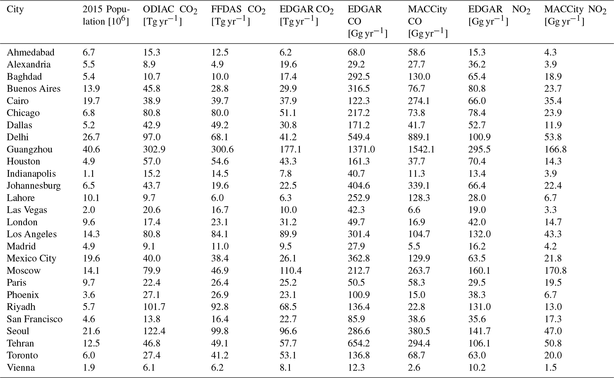
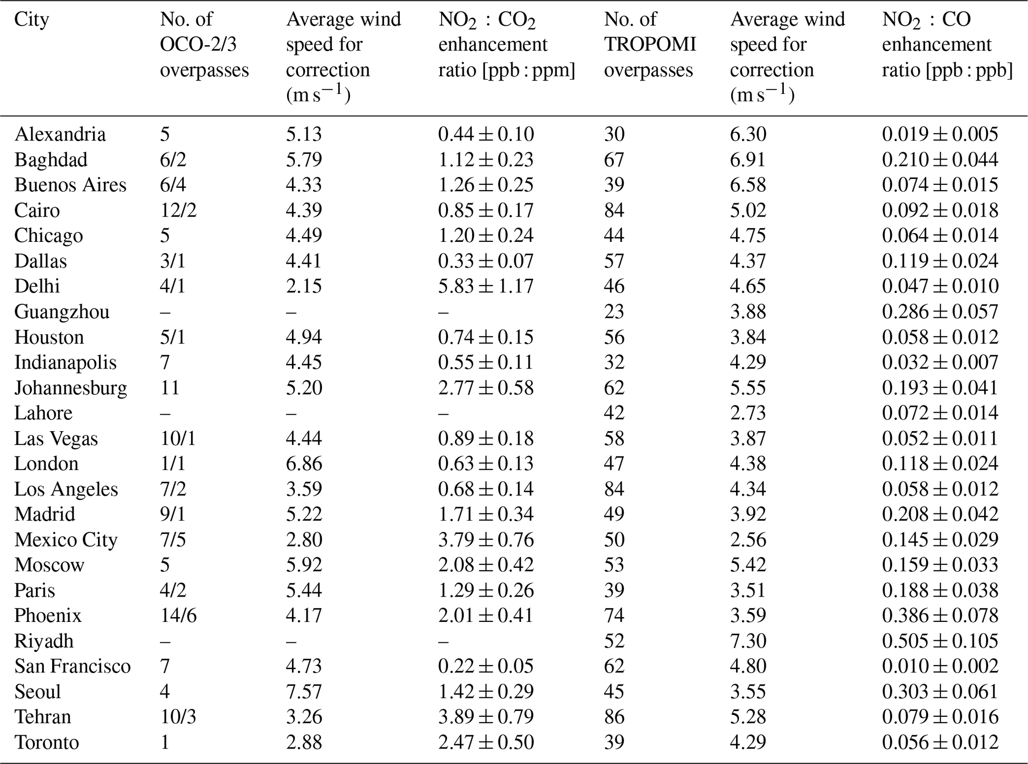
The final inventory that is used is Mapping Atmospheric Chemistry and Climate and CityZen (MACCity; Granier et al., 2011). MACCity provides yearly fluxes of CO and NO_x on a 0.5^∘ × 0.5^∘ global grid from 1990–2010. As with the other inventories, MACCity was downscaled to the resolution of ODIAC before city emissions were derived. Table 1 summarizes emissions estimates from these inventories for all cities that are considered in this study.

Table 1 Summary of inventory-based emissions estimates for all the cities that were considered. Gridded emissions are summed across the extent of the GHS polygon for each city. For the ODIAC and MACCity inventories, which are provided at a monthly temporal resolution, the estimate is the mean across all 12 months.

3 Methods

3.1 Co-location of OCO-2 and TROPOMI data

Because OCO-2 and S5P have Sun-synchronous orbits with similar Equator crossing times and repeat cycles, there is often overlap between observations from the two instruments. We locate overpasses of cities by searching for OCO-2 observations within 75 km of a city boundary of interest. Winds at 50 m are chosen to represent the boundary layer and are used to filter overpasses. We interpolate from the Modern-Era Retrospective analysis for Research and Applications version 2 (MERRA-2; Molod et al., 2015) at a spatial resolution of 0.5^∘ latitude × 0.625^∘ longitude and 3-hourly temporal resolution to the location and time of the overpass. When the boundary layer wind direction does not intersect the OCO-2 ground track, the overpass is rejected, as the pollution plume from the city will not be captured. Further filtering is performed to remove overpasses where the OCO-2 data downwind of the city is extremely sparse (>95 % of OCO-2 observations near the city are flagged as “bad”), which is often the case when there is significant cloud cover in the region. After these filtering steps, the OCO-2 data, along with the TROPOMI data from the same time period, are visualized and inspected to check for issues such as the presence of secondary sources of greenhouse gases or pollutants and to ensure there are spatially coincident measurements between the two satellites. Secondary sources from cities are identified using the European Commission Joint Research Centre's (EC JRC) Global Human Settlement Urban Centre Database (GHS-UCDB) (Corbane et al., 2018). Secondary sources from power plants are identified using the Carbon Monitoring for Action (CARMA) database (Ummel, 2012). During this step, corrections are applied to the MERRA-2 wind direction if considerable discrepancies are observed between the given wind bearing and the behaviour of the plume emanating from the city, which is generally most visible in the TROPOMI NO₂ product. Similar manual corrections have been employed in past studies using observations from OCO-2 (e.g., Nassar et al., 2017; Reuter et al., 2019; Nassar et al., 2021); these errors in wind direction can be caused by the inability of the coarse model resolution to resolve local topography or if the 50 m winds are not representative of the winds at the local plume height. The wind rotation we perform should at least partially correct for both these errors. To compute enhancement ratios, coincident TROPOMI CO and NO₂ enhancements are selected at the locations of the OCO-2 ground track (Fig. 1). At best, our manual inspections found that 83 % of the overpasses which passed the initial automatic filtering were viable in a city, and at worst, all of the overpasses were rejected for a city. The median retention rate is 31 % of the overpasses per city.

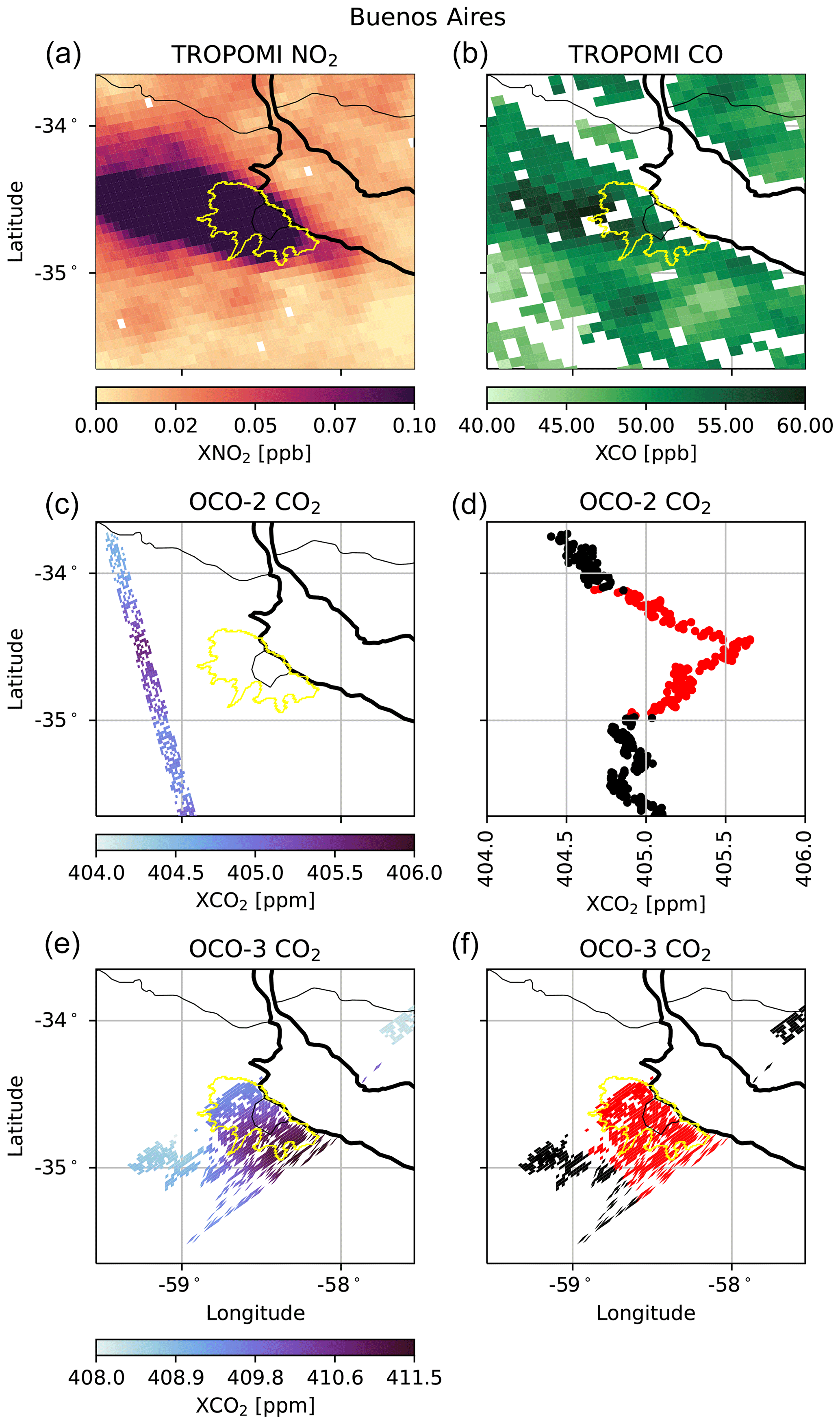
Figure 1 Examples of the various satellite instrument ground tracks over Buenos Aires taken on 11 January 2019 (a–d) and 19 September 2019 (e, f). The yellow outline indicates the city boundaries. The top two panels show the TROPOMI NO₂ (a) and CO (b). The middle two panels show the OCO-2 ground track downwind of Buenos Aires (c) and the CO₂ measurements as a function of latitude (d). Red points indicate the urban enhancement plume, and black points are considered outside the plume. The bottom two panels show the OCO-3 snapshot area mapping (SAM) mode measurements over Buenos Aires (e). Panel (f) distinguishes the region of enhanced CO₂ in red from the background region in black.

A similar approach is used to search for co-located measurements from OCO-3 and TROPOMI. This task is more complex as the ISS is in a different type of orbit than OCO-2 and S5P and thus does not consistently take co-located measurements with the instruments in Sun-synchronous orbits. This can lead to much greater time differences between co-located OCO-3 and TROPOMI measurements compared to the differences between observations from OCO-2 and TROPOMI. Upon identifying a favourable OCO-3 overpass map of a city, the TROPOMI track which lies closest to the city is selected. Time offsets are as large as 6 h between observations from the two instruments. This leads to greater uncertainties in cases where the wind direction has changed significantly in the time between overpasses, as the regions that are affected by the city's plume may no longer coincide with one another. Coincident TROPOMI enhancements are selected at the locations of the OCO-3 SAM measurements (Fig. 1).

Finding instances of co-located measurements of NO₂ and CO from TROPOMI is a far simpler task. Here we search for instances of measurements directly over each city of interest, leading to one or sometimes even two overpasses per day, depending on the longitude of the ground tracks. Due to this much higher data volume, only direct observation of the cities within their bounding areas are considered when deriving NO₂ : CO enhancement ratios to avoid including measurements which are not influenced by the cities due to wind direction errors and lifetime effects. Figure 1 provides example measurement footprints from OCO-2, OCO-3 and S5P's TROPOMI instrument.

3.2 Identifying enhancements

To identify the subset of measurements which are influenced by emissions from the city, we transform the latitude–longitude positions of the observations into along- and cross-wind distances from the city centre and use the equation for the spread of a vertically integrated Gaussian plume, defined by Krings et al. (2011) as

$$\begin{array}{}\text{(2)}& {\mathit{\sigma }}_y=a({\displaystyle \frac{x+x_{\mathrm{0}}}{x_{\mathrm{c}}}}{)}^{\mathrm{0.894}},\end{array}$$

where x is the downwind distance in metres; x_c=1000 m is a characteristic length scale; and a is the atmospheric stability parameter (Pasquill, 1961; Krings et al., 2011; Nassar et al., 2017, 2021), which controls the spread of the plume based on the observed MERRA-2 50 m wind speed so that the plume changes width depending on the wind speed and insolation. Following Nassar et al. (2017), we use the Pasquill–Gifford stability class to determine the atmospheric stability parameter (Martin, 1976), and as in Nassar et al. (2021), we assume solar insolation to be strong given the clear-sky requirements for dense OCO-2/3 observation. The distance x₀ is used to define the initial width of the plume and is defined by

$$\begin{array}{}\text{(3)}& x_{\mathrm{0}}=x_{\mathrm{c}}({\displaystyle \frac{y_{\mathrm{0}}}{\mathrm{4}a}}{)}^{\frac{\mathrm{1}}{\mathrm{0.894}}},\end{array}$$

where y₀ is the cross-wind extent of the city in metres. The factor of 4 in the definition of x₀ follows the method of Krings et al. (2011) so that the cross-wind extent of the city is associated with a ±2σ_y(x₀) spread of the plume. Downwind observations with cross-wind distances that are less than 2σ_y(x) from the mean path from the city y are considered to be in the plume. In cases where the winds point parallel to the affected OCO-2 track, a maximum downwind distance for the plume is determined manually, following Nassar et al. (2017, 2021), to visually identify a drop in $X_{{\mathrm{CO}}_{\mathrm{2}}}$, which limits the length of the plume to an area where significant enhancements are observed.

For comparisons between the TROPOMI NO₂ and CO products, where we do not consider a plume region, the enhancement area is taken as the bounding box of the GHS polygon for the city.

3.3 Anomaly calculation

3.3.1 Smoothing of urban-influenced data

To decrease the amount of noise in the OCO-2/3 and TROPOMI data, we apply a nearest-neighbour fit with a constant radius to smooth out the data (Altman, 1992). For the narrow swath width of OCO-2, we find that fitting a surface to the OCO-2 time series and using a radius of 2 s (equivalent to about six rows of OCO-2 measurements) leads to a fit that removes high-frequency noise but retains the overall trends (Fig. 2). Due to the wide swath width of TROPOMI, it is more appropriate to fit a spatial surface to the data. We find that using a radius of 15 km effectively smooths the data and is comparable in spatial extent to the smoothing applied to the OCO-2 data. Fitting these surfaces to the datasets has the added advantage that predictions can be made at locations which do not have direct measurements but have adequate nearby coverage. This lessens the impact of spurious missing data when trying to find co-located measurements.

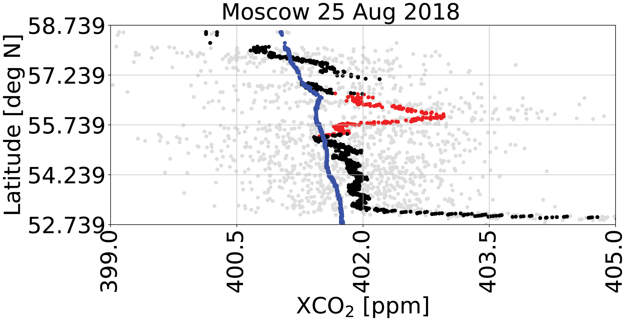
Figure 2 An example of the background and anomaly calculation procedure for OCO-2 data over Moscow (Russia) on 25 August 2018. The grey points represent the original measurements from the OCO-2 Lite files. The OCO-2 ground track in this example is downwind of the city and perpendicular to the wind direction. The black and red points indicate the smoothed data, with the red points corresponding to where the Gaussian plume intersects the OCO-2 track. We consider the red points to be within the urban enhancement plume of the city. The blue line shows the derived background using the lowest 75 % percent of data.

3.3.2 Background calculation

A regional background for $X_{{\mathrm{CO}}_{\mathrm{2}}}$ is determined using nearby measurements from OCO-2 that are free from anthropogenic influence. A nearest-neighbour fit similar to that used to smooth the urban-influenced data is applied here but with a much larger radius of 20 s (approximately 140 km). This choice of radius creates a background whose extent is similar to those in the simulations performed by Wu et al. (2018). The background fit is performed using typically the lowest 75 % of the retrievals so that potential enhancements are removed. For some individual overpasses, the choice of percentage must be tuned if the nearest-neighbour background fit gives a trend that appears to be too high or too low compared to nearby observations which are unaffected by any urban plumes. The performance of this method appears to be most accurate when winds run perpendicular to the OCO-2 track and there exist dense soundings both prior to and after crossing the plume of the city; however satisfactory results were still found in cases where soundings were missing on one side of the plume, which is often the case when cities close to a body of water are observed in nadir mode. Figure 2 shows an example of the process of smoothing the data, identifying an enhancement and calculating the background for an overpass of Moscow with OCO-2.

A similar method is used to define the background for TROPOMI. A radius of 150 km is used for this fit, again using only the lowest 75 % of data to avoid the influence of anthropogenic enhancements on the background. Due to the larger swath width and generally more dense measurements of the TROPOMI products, we find the value does not need to be tuned from 75 % for individual overpasses.

3.3.3 Calculation of anomalies

Anomalies are calculated by subtracting the background estimates from the smoothed urban-influenced values. Coincident observation locations are then chosen using the locations from the sparser of the two species being investigated. For example, if a ratio between CO and CO₂ is being determined, the observation locations from OCO-2 or OCO-3 are used, as their spatial coverage is much smaller than that of the TROPOMI CO product (Fig. 1).

The CO₂ anomalies are divided by the column averaging-kernel values at the surface pressure of the measurement, which is similar to the method used by Wunch et al. (2009) to account for the sensitivities of the instruments to changes in trace gas concentrations near the surface of Earth, where the emissions from cities originate. We must also account for the fact that the TROPOMI a priori profiles of NO₂ and CO are extracted from the Tracer Model version 5 (TM5-MP, Williams et al., 2017) chemical transport model and thus contain spatial information such as urban enhancements. This requires that an additional correction term is added when inferring the true enhancement Δc^t from the retrieved enhancement $\mathrm{\Delta }\widehat{c}$ if the urban and background a priori total columns $c_{\mathrm{u}}^{\mathrm{a}}$ and $c_{\mathrm{b}}^{\mathrm{a}}$ and the surface pressure column averaging kernels a⁰ are known:

$$\begin{array}{}\text{(4)}& \mathrm{\Delta }{c}^{\mathrm{t}}={\displaystyle \frac{\mathrm{\Delta }\widehat{c}}{a^{\mathrm{0}}}}-{\displaystyle \frac{(\mathrm{1}-a^{\mathrm{0}})(c_{\mathrm{u}}^{\mathrm{a}}-c_{\mathrm{b}}^{\mathrm{a}})}{a^{\mathrm{0}}}}.\end{array}$$

Figure 3 demonstrates this anomaly calculation procedure, and Fig. 4 shows an example of the distributions of surface averaging kernels for the three gases that are considered. Appendix C describes the averaging-kernel correction in detail.

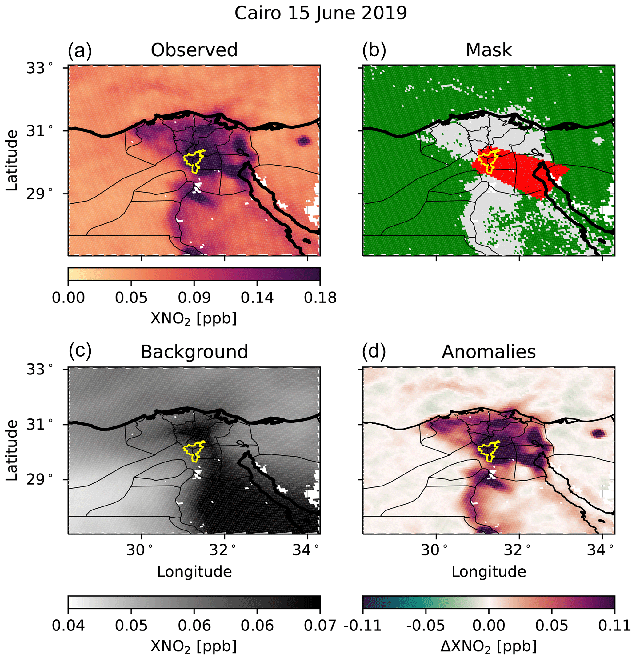
Figure 3 An example of the background and anomaly calculation procedure for TROPOMI NO₂ observations over Cairo on 15 June 2019. Panel (a) shows the smoothed set of observations. Panel (b) shows the mask for the background calculation; green points are below the 75th percentile and used in the calculation, while grey points are omitted, and red points indicate observations in the enhancement. The selection of the enhancement region is done liberally, as the location of OCO-2/3 observations is often a more limiting factor. Panel (c) then shows the derived background, and panel (d) shows the calculated anomalies. The extent of the GHS polygon for Cairo is shown in yellow. Thick black lines mark coastlines, and thin black lines indicate geopolitical boundaries.

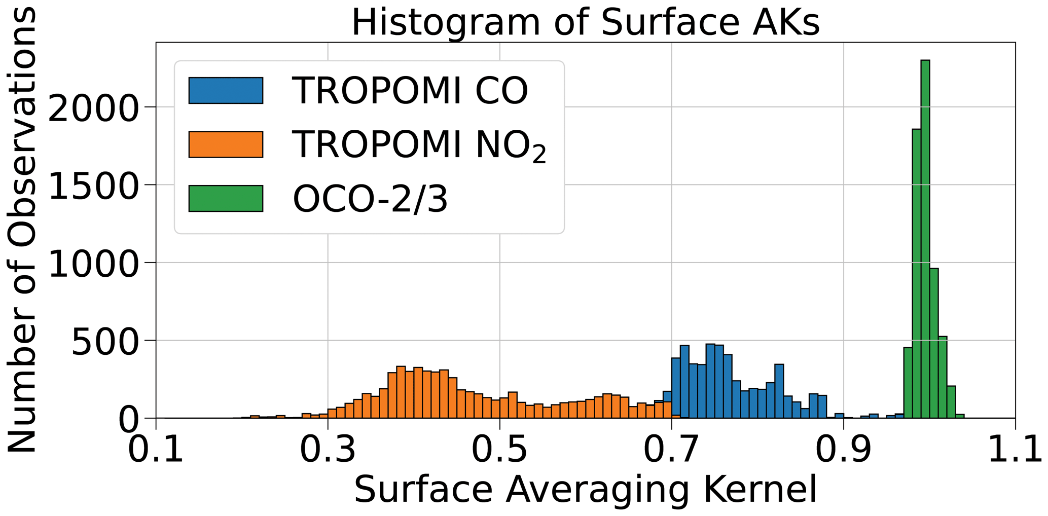
Figure 4 Example histograms of the averaging-kernel (AK) values at the surface pressure for OCO-2/3 and TROPOMI from all the data collected over Phoenix (USA), which are used to account for the sensitivity of the instruments to concentration changes at the surface.

3.4 Determination of enhancement ratios

To determine enhancement ratios, we aggregate all overpasses for a given city and regress one set of anomalies onto the other using a reduced major-axis regression as described by York et al. (2004), as shown in Fig. 5. The variance of the samples is used as the uncertainty for each observation. Reduced major-axis regression has the property that the resulting slope is independent of which variable is chosen to be on the abscissa and which is chosen to be on the ordinate axis. Furthermore, the calculated slope is unaffected by the scaling of axes by a constant value so that the calculated slopes are independent of the choice of mixing ratio units that are used (i.e., ppm or ppb). This method is then bootstrapped (Efron and Gong, 1983) 500 times to get an error estimate for the fit. Bootstrapping is a resampling technique in which random pairs of anomalies are drawn with replacement and fit independently and has been used in previous enhancement ratio studies (e.g., Wunch et al., 2009, 2016; Lama et al., 2020). We take twice the standard deviation of the resulting set of slopes as the uncertainty estimate for the fit.

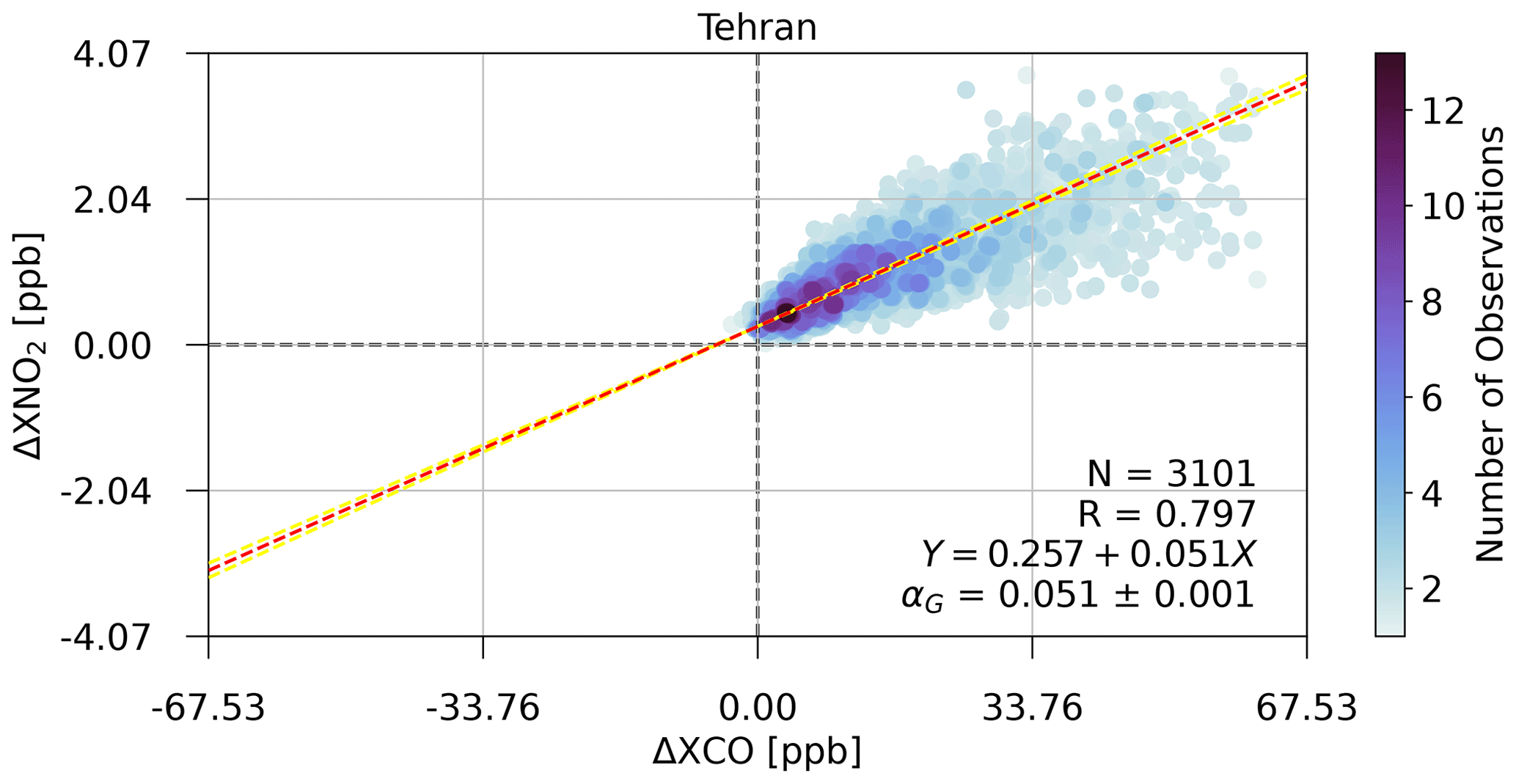
Figure 5 Regression of anomalies of $X_{{\mathrm{NO}}_{\mathrm{2}}}$ onto anomalies of X_CO over Tehran using TROPOMI data from June–August 2018. The dashed red line indicates the estimated enhancement ratio, while the yellow lines represent ±2σ uncertainties in the ratio. Each data point represents a single observation and is assigned a colour to indicate the density of points by binning the observations into 100 bins across each axis and counting the number of points in the bin in which the observation resides. N is the total number of points included in the regression, R is the correlation coefficient, Y is the equation of best fit, and α_G is the slope and 2σ uncertainty determined by bootstrapping.

3.5 NO₂ lifetime correction

NO₂ has a short atmospheric lifetime compared to those of both CO₂ and CO and can be on the same order as the advective timescales associated with emissions on the scale of large cities. To account for this, we apply a correction to the observed enhancement ratios to model the effect of NO₂ lifetime. Following Lutsch et al. (2020), the multiplicative correction takes the form

$$\begin{array}{}\text{(5)}& C=\exp ({\mathit{\tau }}_{\mathrm{A}}/{\mathit{\tau }}_{{\mathrm{NO}}_{\mathrm{2}}}),\end{array}$$

where τ_A is a timescale for advection and ${\mathit{\tau }}_{{\mathrm{NO}}_{\mathrm{2}}}$ is the lifetime of NO₂. This uses the fact that the chemical loss of NO₂ can be modelled as ${\mathrm{NO}}_{\mathrm{2},\mathrm{orig}}\cdot \exp (-t/{\mathit{\tau }}_{{\mathrm{NO}}_{\mathrm{2}}})$. Thus, when t=τ_A, the ratio is ${\mathrm{NO}}_{\mathrm{2},\mathrm{orig}}/{\mathrm{NO}}_{\mathrm{2},\mathrm{downwind}}=C$. We use the method described in Laughner and Cohen (2019) to calculate NO₂ lifetimes for each city separately for summer and winter (details given in Appendix B). We apply a single lifetime correction by scaling the observed enhancement ratio so that α_Corrected=Cα, with an advection timescale given by

$$\begin{array}{}\text{(6)}& {\mathit{\tau }}_{\mathrm{A}}={\displaystyle \frac{\mathrm{1}}{\stackrel{\mathrm{‾}}{U}}}({\displaystyle \frac{A}{\mathit{\pi }}}{)}^{\mathrm{1}/\mathrm{2}},\end{array}$$

where $\stackrel{\mathrm{‾}}{U}$ is the average wind speed averaged across all overpasses of the city and weighted by the number of observations in each overpass and A is the area of the city provided in GHS-UCDB so that the relevant length scale is the radius of the city if it were a perfect circle with area A. In applying these corrections, we have neglected the lifetimes of CO and CO₂, which are on the order of months and centuries, respectively, and therefore will have a negligible effect on the observed enhancement ratios. To account for errors in the NO₂ lifetimes as well as the wind speeds used to calculate the advective timescales, we add an additional 20 % in quadrature to the initial enhancement ratio uncertainty when the lifetime correction is applied.

4 Results

4.1 NO₂ : CO₂ and CO : CO₂ ratios

Using these methods, we are able to quantify NO₂ : CO₂ ratios from 22 cities and CO : CO₂ ratios from 21 cities using co-located observations from TROPOMI, OCO-2 and OCO-3. A total of 174 overpasses occurring from April 2018 to May 2020 are used to derive NO₂ : CO₂ ratios, with 140 consisting of observations from TROPOMI and OCO-2 and the remaining 34 involving TROPOMI and OCO-3. The most overpasses for an individual city are found for Phoenix (USA), where we found 20 usable overpasses; Toronto has the fewest, where only a single overpass is used. In many cases, overpasses involving OCO-3 had to be filtered out due to observed non-linear relations between the derived $X_{{\mathrm{CO}}_{\mathrm{2}}}$ anomalies and those from the two TROPOMI products for a given day. This issue is most likely caused by the greater time differences between overpasses of the ISS and S5P – the location and distribution of the plumes could change significantly between the two times at which measurements are made so that the measurements are no longer approximately co-located in time and space.

Cities located in the southwestern United States (Los Angeles, San Francisco, Phoenix and Las Vegas) and in the Middle East (Tehran, Baghdad and Cairo) generally yielded more usable overpasses than cities located elsewhere in the world due to the greater number of cloud-free daylight hours in these regions. Few good overpasses were found for cities located in East Asia and Southeast Asia, as observations from OCO-2/3 are often very sparse due to persistent clouds; other than Guangzhou (China) and Seoul (South Korea), megacities in these regions of the globe are not considered in this study. Overpasses were also generally better for inland cities compared to those situated next to large bodies of water, where loss of data from nadir viewing in the OCO-2/3 product and data filtering in the TROPOMI CO product led to more limited opportunities to make observations downwind of the city. The presence of mountains near cities also presented some problems; in such cases large corrections to the reported MERRA-2 wind directions were often required to properly capture the plume. In the unique case of Los Angeles and the SoCAB in which the city resides, we considered only measurements directly above the SoCAB in our analysis, as the surrounding mountain ranges prevent air in the urban boundary layer from easily leaving the basin.

Figure 6 CO : CO₂ enhancement ratios derived using observations from OCO-2/3 and TROPOMI compared to inventory estimates using CO emissions from EDGAR and CO₂ emissions from EDGAR, FFDAS and ODIAC. The numbers on top of the bars denote the correlation coefficient between the two sets of observed anomalies. The error bars atop the bars represent the uncertainty in the measured ratios.

Figure 6 shows the derived CO : CO₂ enhancement ratios from our analysis compared to inventory-based estimates of the enhancement ratios derived from the ODIAC, FFDAS and EDGAR emissions inventories. For cities across the United States, Canada and Europe, we find that apart from the Dallas–Fort Worth area, our measured enhancement ratios are higher than the inventory-based estimates, with our results ranging from around 1.1 (Phoenix) to 4.7 (Paris) times greater than the respective EDGAR estimates. Results for the remainder of the cities show a less consistent picture, with the largest underestimate being for Baghdad (Iraq), where we find an enhancement ratio that is around 3 times lower than that of the EDGAR estimate and the largest overestimate for Tehran, where the measured enhancement ratio is around 1.6 times greater than the EDGAR value. When comparing to ratios calculated using CO emissions from the MACCity inventory, shown in Appendix A, we find a more pronounced underestimation compared to observations across North America and Europe.

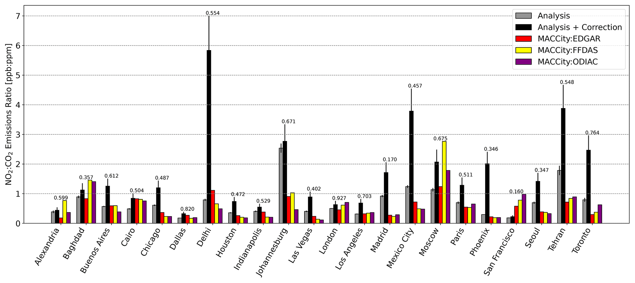
Figure 7 Same as in Fig. 6 but for NO₂ : CO₂ ratios derived using OCO-2/3 and TROPOMI observations. NO₂ enhancements calculated without a lifetime correction are in grey and labelled “analysis”, and those with a lifetime correction are in black and labelled “analysis + correction”.

Figure 7 similarly shows results for the derived NO₂ : CO₂ ratios, both with and without the correction for NO₂ lifetime. Here we find that without any NO₂ lifetime correction, almost all of the cities considered have derived ratios that are smaller than the inventory-based estimates. As with the CO : CO₂ results, this discrepancy is most pronounced in the United States and Europe. Upon applying our lifetime correction to the ratios, the ratios in many of these cities are brought closer to the inventory-based estimates, with a few cities (Delhi, Mexico City and Tehran) having ratios that are higher than any of the inventory estimates. Delhi has a particularly low wind speed (Table 3), which may cause the NO₂ lifetime correction to be overestimated. Additionally, correlation coefficients between the two sets of anomalies were generally found to be greater in this case when compared to the CO : CO₂ enhancement ratio results. Ratios calculated using the MACCity inventory, shown in Appendix A, show better agreement with those derived using satellite observations prior to the application of the lifetime correction, but observed enhancements are generally higher than the inventory estimates after the atmospheric lifetime correction is applied.

4.2 NO₂ : CO ratios

We also derive NO₂ : CO ratios for the same cities using only measurements from TROPOMI. Because NO₂ : CO enhancement ratios do not use observations from OCO-2/3, which have more limited coverage, there are far more opportunities for calculating these ratios. In the absence of cloud cover, we obtain one to two overpasses per day for each city. We consider a smaller subset of the TROPOMI product from June–August 2018, which is the same subset of data used by Lama et al. (2020) so that our enhancement ratios are derived from 23–86 overpasses for each city. Because there are more overpasses averaged into the NO₂ : CO estimates of enhancement ratios, we expect them to be more robust than those involving OCO-2/3.

Figure 8 shows the derived NO₂ : CO ratios compared to inventory-based estimates from EDGAR and MACCity. Here we observe ratios that are significantly lower than inventory-based estimates both before and after the lifetime correction has been applied. Again these differences are generally more significant over cities in North America and Europe, and Johannesburg and Baghdad are outliers, with observed enhancement ratios higher than either of the inventory estimates. Tables 2 and 3 summarize the results of all three sets of emissions ratios for all the cities considered. Figure 10 shows the median relative difference between our enhancement ratios and those derived from inventories.

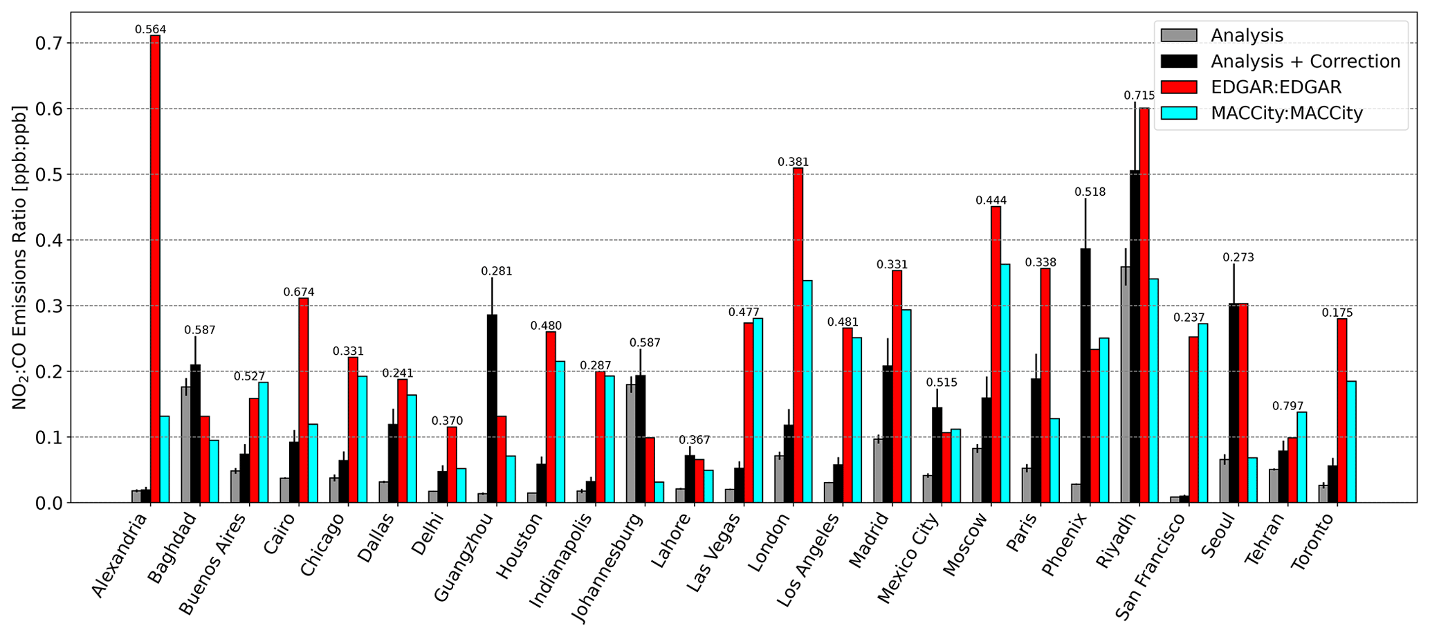
Figure 8 Same as in Fig. 6 but for NO₂ : CO ratios derived using observations from TROPOMI. EDGAR and MACCity are used to calculate inventory-based estimates of the emissions ratios.

Table 2 All enhancement ratios derived using OCO-2/3 and TROPOMI. Overpasses must individually have sufficient linear dependence (R>0.2). Cities without any such overpasses are marked by a dash.

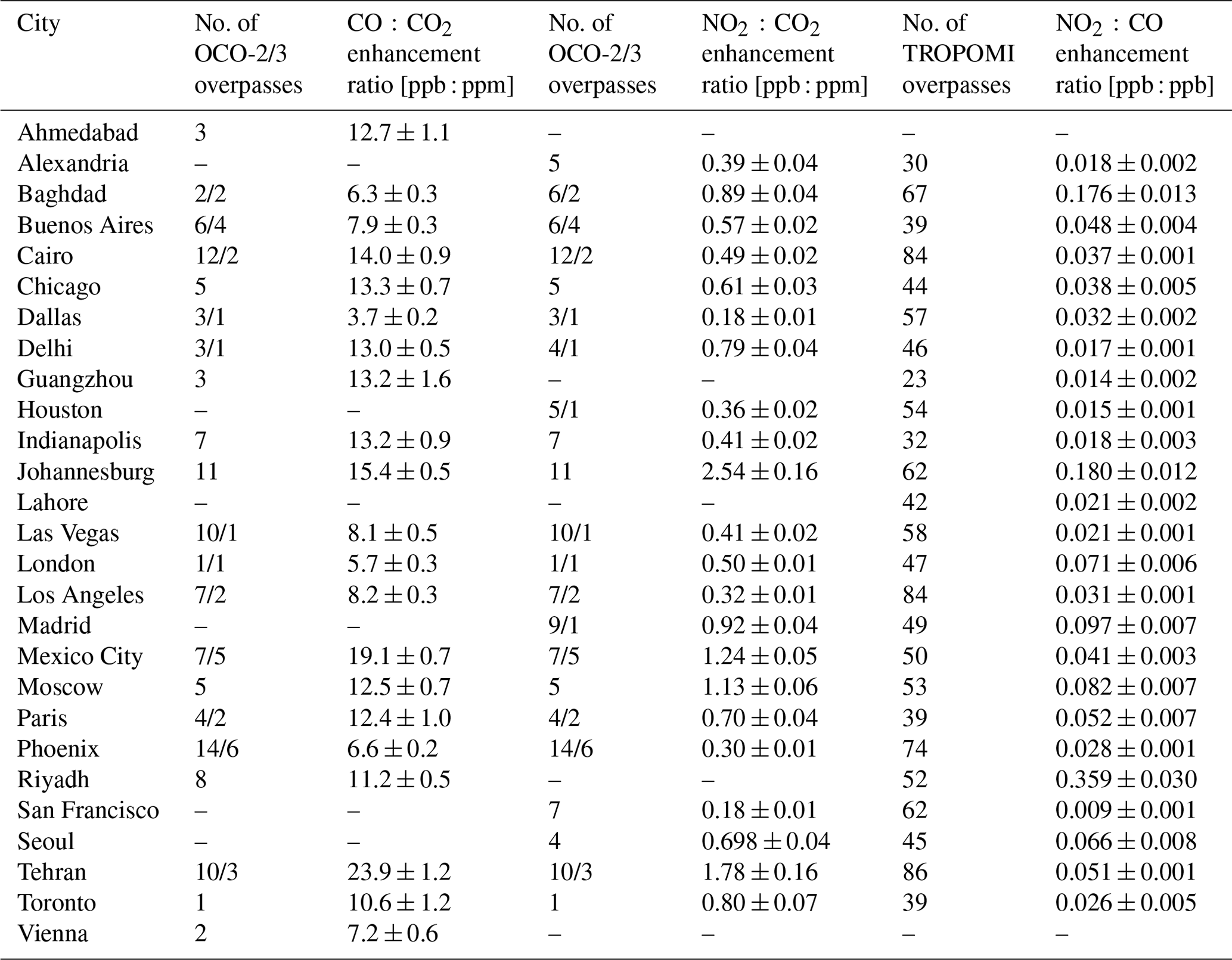
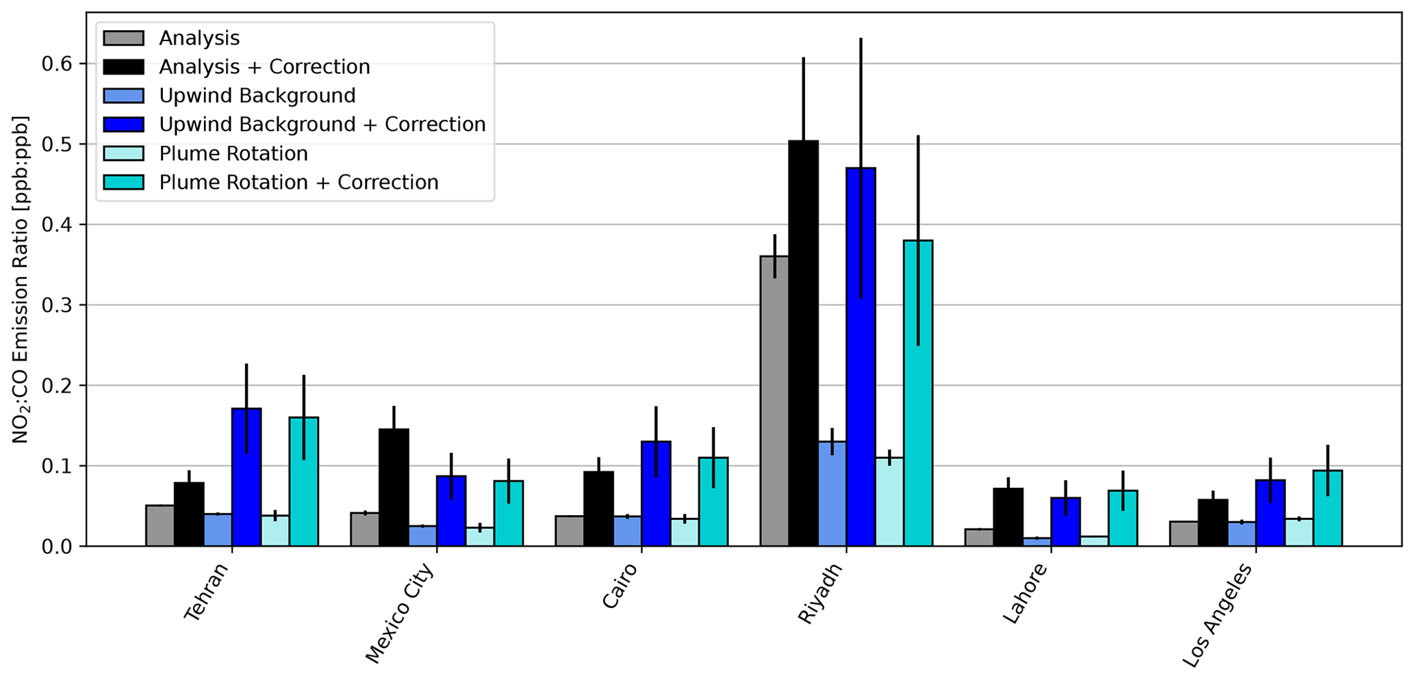
Figure 9 Comparison of our observed NO₂ : CO ratios (analysis and analysis + correction) to those calculated by Lama et al. (2020). Lama et al. (2020) use two different methods to compute enhancements: their “upwind background” method and their “plume rotation” method. Both are shown here, with and without their respective lifetime corrections.

We also compare our NO₂ : CO results to those of Lama et al. (2020) in Fig. 9. Lama et al. (2020) applied two different methods to calculate NO₂ : CO enhancement ratios in six megacities (Tehran, Mexico City, Cairo, Riyadh, Lahore and Los Angeles) using measurements from TROPOMI. Lama et al. (2020) also use an averaging-kernel correction with their ratios, except with a different methodology; they apply column averaging kernels to reported profiles of NO₂ and CO from the Copernicus Atmospheric Monitoring Service (CAMS) to determine the impact on $X_{{\mathrm{NO}}_{\mathrm{2}}}$ and X_CO. Lama et al. (2020) also apply a correction which accounts for the short lifetime of NO₂ due to chemical reactions with hydroxyl (OH) in the atmosphere by constructing a correcting scale factor using CAMS-reported OH concentrations and the observed wind speed. Comparing the results of Lama et al. (2020) to our calculated values without their respective NO₂ lifetime corrections, we find good agreement, within the uncertainties, in the ratios for all cities except Riyadh. After the application of the respective NO₂ lifetime corrections, all cities except Tehran show agreement within the uncertainties. Our NO₂ lifetime correction is significantly smaller in Tehran than the Lama et al. (2020) correction.

Table 3 All NO₂ : CO₂ and NO₂ : CO enhancement ratios derived using OCO-2/3 and TROPOMI, including the NO₂ lifetime correction. Overpasses must individually have sufficient linear dependence (R>0.2). Cities without any such overpasses are marked by a dash.

5 Discussion

5.1 Analysis of measured ratios

The CO : CO₂ ratios that we derive using TROPOMI and OCO-2/3 are larger than the inventory-based estimates calculated from EDGAR, ODIAC and FFDAS in 71 % of the cities we studied (Fig. 6). This is the case for nearly all cities in North America and Europe, though mixed results are observed for the rest of the world; in cities such as Tehran (Iran) and Cairo (Egypt) we observe high ratios relative to inventory estimates, while in Johannesburg (South Africa), Baghdad (Iraq) and Buenos Aires (Argentina), we observe ratios that are lower than the inventory values. We also observe larger CO : CO₂ enhancement ratios relative to reported emissions ratios when using CO emissions from the MACCity inventory (Fig. A1 in Appendix A). Here, the low bias for inventory estimates appears to be even stronger for cities in North America and Europe, while Johannesburg and Baghdad remain as outliers with lower observed enhancement ratios.

Figure 10 The median relative difference in percent between the observed enhancement ratios and those from the inventories (inventory − observed). The leftmost set of bars is for the CO : CO₂ enhancement ratios. The middle set of bars is for lifetime-corrected NO₂ : CO₂ enhancement ratios, and the right set of bars is for lifetime-corrected NO₂ : CO enhancement correction. The error bars show the standard deviation in the spread in inventory differences from the measurements over all cities divided by the square root of the number of cities.

For the NO₂ : CO₂ ratios that we calculate (Fig. 7), we find that without any correction for NO₂ lifetime, this trend is reversed: we observe ratios that are considerably lower than those derived from EDGAR, ODIAC and FFDAS in 91 % of the cities. Upon application of our correction for NO₂ lifetime, the ratios for many of these cities are brought in closer agreement with the inventory estimates. Johannesburg is a notable outlier, with an observed ratio that is comparable to the EDGAR and FFDAS estimates both before and after correction yet is around twice the EDGAR : ODIAC estimated ratio. Delhi, Mexico City and Tehran also have ratios that exceed inventory-based estimates by a similar amount after the lifetime correction has been applied. An added complication for the specific case of Johannesburg is the presence of a collection of large coal-fired power plants located ∼ 100 km east of the city which together emit >10 Tg CO₂ yr⁻¹ and an additional two power plants located ∼ 50 km to the south according to the Carbon Monitoring for Action (CARMA) database (Ummel, 2012). Plumes from these sites are clearly visible in CO and NO₂ measurements from TROPOMI and depending on the wind direction and distance from the city could influence the measurements in the OCO-2 swath. Interestingly, the positions of these four cities (Delhi, Johannesburg, Mexico City, Tehran) as outliers appears to be consistent for both EDGAR NO_x emissions and those from MACCity.

In general, we find that measured NO₂ : CO enhancement ratios are smaller than those inferred from the inventories, while measured CO : CO₂ ratios are generally larger than those from the EDGAR, FFDAS and ODIAC inventories (Fig. 10). Measured NO₂ : CO₂ ratios are in reasonable agreement with the inferred inventory enhancement ratios using EDGAR NO₂ (Fig. 10). From our observed CO : CO₂ ratios, which are generally larger than the inventory ratios, we infer that the inventories we considered tend to either underestimate CO emissions, overestimate CO₂ emissions or both. Similarly, the lifetime-corrected NO₂ : CO₂ ratios that are observed to generally agree with the EDGAR NO_x-based estimates suggest either that the inventories accurately capture emissions of both NO₂ and CO₂ or that emissions of these two gases are both biased either high or low by a similar magnitude. Given that the spread provided by the three CO₂ inventories (which is on average about 20 % around the mean of the three and exceeds 30 % for only Alexandria, Delhi, Johannesburg and Moscow) coincides with the uncertainty range for the NO₂ : CO₂ enhancement ratio in 8 out of 22 cities and is close for another 7 cities, the NO₂ : CO₂ emissions ratios do not appear to be affected by systematic biases as much as the CO : CO₂ ratios. From this, we infer that the discrepancies in the NO₂ : CO ratios are likely caused by an underestimation of CO emissions within the EDGAR inventory. The MACCity NO₂ : CO ratios are also larger on average than the measured enhancements, but both CO : CO₂ and NO₂ : CO₂ enhancement ratios are smaller than the measured enhancements (Figs. 10, A1 and A2). This is consistent with the mean MACCity CO emissions being lower than EDGAR CO emissions by about 20 % in the cities we have studied, while its mean NO₂ emissions are less than half of those reported by EDGAR in these cities (Table 1).

If we were to rescale the CO inventory emissions so that their emissions ratios matched the observed CO : CO₂ enhancement ratios, EDGAR CO emissions would have to be about doubled on average. For MACCity, the required rescaling factor is considerably higher; this was driven in part by the CO emissions estimates in Riyadh (Saudi Arabia), Las Vegas (USA) and Phoenix (USA). This suggests that MACCity may systematically underestimate CO emissions in desert cities. Even when neglecting these three cities, the low-biased emissions in MACCity would still require a rescaling factor of around 4 on average to match the observed enhancement ratios.

One potential source of error in this analysis is from biogenic emissions of CO and cycling of CO₂, but we expect these effects will be small. Under the assumption that there is less vegetation within urban boundaries than outside the urban region, biogenic CO and CO₂ emissions have the potential to affect the urban–rural gradients, especially during the growing season. According to recent studies, however, these gradients are significantly smaller than the enhancements we measure, suggesting that urban CO and CO₂ enhancements are dominated by fossil fuel emissions (Plant et al., 2022b; Wu et al., 2022). Further modelling will be necessary to apply this kind of analysis to smaller emissions sources.

A second possible source of error is the temporal representativeness of the satellite data used in this analysis. The overpasses that successfully pass our filtering criteria are biased toward sunnier conditions and are most often collected in summertime, and some sites have very few overpasses (e.g., Toronto). If the enhancement ratios change seasonally, as might be expected, this type of analysis could cause a representativeness error, in which the comparisons between the measured enhancement ratios and the reported annual inventory ratios are systematically biased. Currently, the EDGAR and MACCity inventories, which provide CO and NO₂ emissions, do not report sub-annual emissions, so comparison to seasonal inventory ratios is not possible. With longer satellite time series providing more opportunities for wintertime enhancement ratios, we will be able to compute robust annual enhancement ratios to compare with the annual inventories.

5.2 Emissions estimates using high-resolution inventories

In addition to the global, gridded inventories that we have employed up to this point, the cities of Indianapolis (USA) and Los Angeles (USA) also have high-resolution anthropogenic CO₂ inventories. The Hestia inventory provides gridded CO₂ fluxes for the cities of Los Angeles, Indianapolis, Salt Lake City and Baltimore at both hourly and annual temporal resolutions for the years 2010–2015 (Gurney et al., 2018b, 2019). The inventory for Los Angeles is provided at a spatial resolution of 1 km × 1 km for the SoCAB and the surrounding area, and the inventory for Indianapolis is given on a 200 m × 200 m grid. When summed across the GHS polygons for each city, the annual emissions for Los Angeles and Indianapolis from the Hestia inventory are 120.9 and 13.5 Tg CO₂ yr⁻¹, respectively. For Los Angeles, the annual estimates of the global gridded inventories (EDGAR, ODIAC and FFDAS) are between 25 %–33 % lower than this high-resolution estimate, while, for Indianapolis, the Hestia estimate is similar to the mean of the three global inventories. When comparing these with the TIMES-corrected emissions rates from the global inventories for Los Angeles, the estimates are brought into better agreement with the Hestia inventory, with emissions rates that are now only 6 %–17 % lower than Hestia. For Indianapolis, the TIMES-corrected EDGAR estimate of 9.5 Tg CO₂ yr⁻¹ is about 30 % lower than the Hestia estimate, while the ODIAC and FFDAS values are around 30 % higher.

Using the CO : CO₂ enhancement ratio that was calculated for Los Angeles along with the Hestia CO₂ emissions estimate and Eq. (1), we estimate CO emissions to be 635 ± 127 Gg CO yr⁻¹ after assuming a 20 % uncertainty in the Hestia emissions estimate, which has good overlap with the estimate of 487 ± 122 Gg CO yr⁻¹ found by Hedelius et al. (2018) for 2013–2016, as well as the value of 581 Gg CO yr⁻¹ for the SoCAB which is reported by the California Air Resources Board (CARB) for the year 2015 in the CARB2017 database (https://www.arb.ca.gov/app/emsinv/2017/emssumcat.php, last access: 10 March 2023). CARB2017 projections for the year 2020 estimate that SoCAB emissions of CO should decrease by 21 %. The EDGAR and MACCity CO emissions estimates for Los Angeles are significantly lower at 301.4 and 104.7 Gg CO yr⁻¹, respectively (Table 1).

In a similar way, we estimate emissions of NO₂ within the SoCAB to be 89 ± 17 Gg NO₂ yr⁻¹ (after the NO₂ lifetime correction is applied), which agrees with the CARB estimate for 2015 of 105 Gg NO₂ yr⁻¹. CARB2017 projections for the year 2020 estimate that SoCAB emissions of NO_x should decrease by 26 %. However, our estimated emissions are smaller than the annual EDGAR estimate of 132 Gg NO₂ yr⁻¹ and larger than the MACCity estimate of 43.3 Gg NO₂ yr⁻¹.

A similar approach using the Hestia CO₂ inventory for Indianapolis yields estimated CO emissions of 115 ± 23 Gg CO yr⁻¹, much higher than both the EDGAR and MACCity estimates of 40.7 Gg CO yr⁻¹ and 11.7 Gg CO, respectively. Using the lifetime-corrected NO₂ : CO₂ ratio, emissions of NO₂ are estimated to be 7.8 ± 1.6 Gg NO₂ yr⁻¹, which is considerably higher than the MACCity estimate of 3.9 Gg NO₂ yr⁻¹ but lower than the EDGAR estimate of 13.4 Gg NO₂ yr⁻¹.

These investigations of Los Angeles and Indianapolis illustrate how the high MACCity NO₂ : CO ratios observed in Fig. 8 are driven by a strong underestimation of CO emissions, even though the NO_x emissions are also underestimated in MACCity compared to the estimate derived from enhancement ratios and Hestia.

6 Conclusions

This study demonstrates a method to derive enhancement ratios between CO₂, CO and NO₂ using measurements from the OCO-2, OCO-3 and TROPOMI satellite instruments located downwind of or over large urban areas. This method is applied to derive enhancement ratios for 27 cities from around the world. These ratios are then compared to enhancement ratios derived from the EDGAR, ODIAC, FFDAS and MACCity global inventories. We find that CO : CO₂ ratios from these inventories are generally lower in cities across Europe and North America compared to the satellite-based ratios. After applying a correction to account for the short atmospheric lifetime of NO₂, observed NO₂ : CO₂ ratios are mostly higher than inventory ratios when using NO_x emissions from MACCity but generally show good agreement when using emissions from EDGAR, apart from a few outlier cities where observed ratios were high compared to inventory estimates. Lifetime-corrected NO₂ : CO ratios retrieved from TROPOMI observations over these cities show low values relative to inventory estimates and good agreement with the lifetime-corrected NO₂ : CO ratios derived in a previous study by Lama et al. (2020).

We demonstrate that deriving enhancement ratios between more than two species can aid in the interpretation of results. By measuring ratios of CO : CO₂, NO₂ : CO₂ and NO₂ : CO, we are able to better diagnose which emissions lead to discrepancies between satellite- and inventory-derived ratios. For the EDGAR inventory, this analysis suggests an underestimation of CO emissions by around 50 % on average, while for the MACCity inventory, we infer a more significant underestimation of CO emissions of about 75 % on average, alongside a smaller underestimation of NO_x emissions. In both EDGAR and MACCity, many of the largest underestimations of CO are observed for cities in Europe and North America, with MACCity showing significant underestimation in desert cities (Riyadh, Phoenix, Las Vegas). Further, we show that by combining these enhancement ratios with high-resolution CO₂ inventories, emissions of CO and NO₂ can be calculated, which, in the case of Los Angeles, shows good agreement with both region-specific inventories and previous modelling studies. These analyses with high-resolution inventories additionally provide further support for the underestimation of urban CO emissions in EDGAR and MACCity.

There is considerable potential for further study using the methodology that has been laid out here. In particular, these methods could be applied to other anthropogenic co-emitters of CO₂, CO and NO₂. Fossil-fuel-burning power plants are a candidate for future investigations, as other studies have already used multi-sensor techniques involving NO₂ and CO₂ to estimate power plant emissions (e.g., Reuter et al., 2019; Hakkarainen et al., 2021). Furthermore, enhancement ratios involving other species observed by TROPOMI, such as CH₄, HCHO and SO₂, over urban regions could be explored using the framework that has been described here.

Due to the limited number of usable co-locations between OCO-2/3 and TROPOMI that were available in this study, we have limited our enhancement ratio results to single values across the full time periods. As the constellation of CO₂-observing satellites expands in the coming years, there will be greater potential for co-locations of observations, which could provide reliable information on long-term trends of these enhancement ratios and open up the possibility for comparison to trends in ratios derived from emissions inventories. When paired with state-of-the-art CO₂ inventories, these enhancement ratios could provide a flexible framework to determine whether emissions reduction targets for a wide array of greenhouse gases and pollutants are being met on schedule by cities around the world.

Appendix A: Comparison of CO : CO₂ and NO₂ : CO₂ ratios with emissions ratios derived from MACCity

Comparison of our observed CO : CO₂ enhancement ratios with emissions ratios calculated using CO emissions from the MACCity inventory are shown in Fig. A1. Results are similar to those using the EDGAR CO emissions, with underestimation by the inventories relative to the observations even more pronounced for many cities in Europe and North America. Similarly, Fig. A2 shows a comparison of observed NO₂ : CO₂ with MACCity-derived emissions ratios. These emissions ratios are characterized by a greater underestimation relative to the observed enhancement ratios when compared with the EDGAR emissions. As with the EDGAR emissions ratios, the cities of Delhi, Johannesburg, Mexico City and Tehran stand out as the cases where this underestimation is the most pronounced.

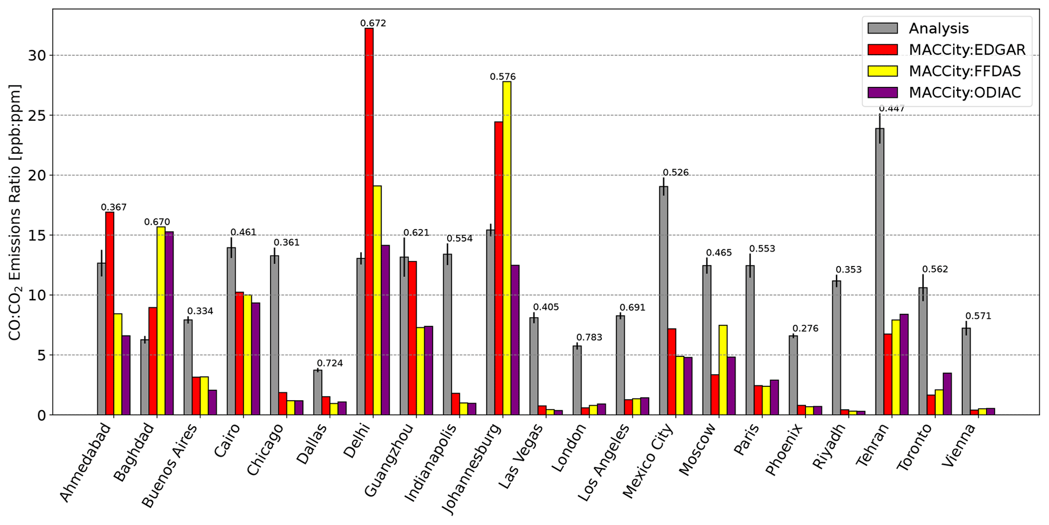
Figure A1 Same as is Fig. 6 but for enhancement ratios calculated using CO emissions from the MACCity inventory.

Figure A2 Same as in Fig. 7 but for enhancement ratios calculated using NO_x emissions from the MACCity inventory.

Appendix B: NO₂ lifetime calculation

We compute NO₂ lifetimes similarly to Laughner and Cohen (2019) using NO₂ column densities from offline TROPOMI data (processor version 1.3). Wind direction for each day is calculated from GEOS-5 FP-IT (forward processing for instrument teams) reanalysis data (Lucchesi, 2015) by interpolating the bottom five levels of the wind fields to 13:30 local time. Horizontal averaging uses a flat-topped Gaussian (fourth-power) function centred on each city, with a width chosen based on the city size. NO₂ column densities from each day are rotated so that the wind directions are aligned, and pixels with qa_value >0.75 are averaged in time, weighted by the pixel area. Line densities are computed by integrating the rotated line densities perpendicular to the wind direction. The exponentially modified Gaussian function

$$\begin{array}{}\text{(B1)}& \begin{array}{rl}F\left(x\right|a,x_{\mathrm{0}},{\mathit{\mu }}_x,{\mathit{\sigma }}_x,B)& ={\displaystyle \frac{a}{\mathrm{2}{x}_{\mathrm{0}}}}\exp \left({\displaystyle \frac{{\mathit{\mu }}_x}{x_{\mathrm{0}}}}+{\displaystyle \frac{{\mathit{\sigma }}_x^{\mathrm{2}}}{\mathrm{2}{x}_{\mathrm{0}}^{\mathrm{2}}}}-{\displaystyle \frac{x}{x_{\mathrm{0}}}}\right)\\ & \cdot \mathrm{erfc}\left(-{\displaystyle \frac{\mathrm{1}}{\sqrt{\mathrm{2}}}}\left[{\displaystyle \frac{x-{\mathit{\mu }}_x}{{\mathit{\sigma }}_x}}-{\displaystyle \frac{{\mathit{\sigma }}_x}{x_{\mathrm{0}}}}\right]\right)\end{array}\end{array}$$

is fit to the line densities. x is the along-wind distance, and a, x₀, μ_x, σ_x and B are fitting parameters; erfc is the error function complement. Lifetime is calculated as $x_{\mathrm{0}}/\stackrel{\mathrm{‾}}{u}$, where $\stackrel{\mathrm{‾}}{u}$ is the average wind speed from GEOS FP-IT.

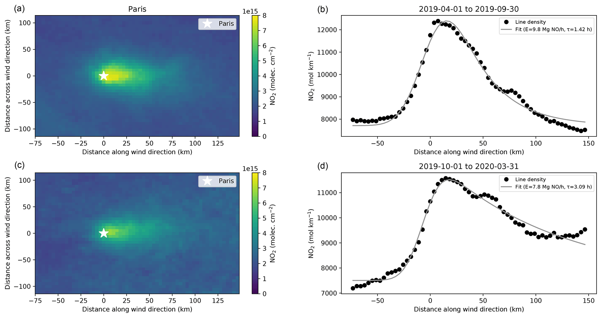
Figure B1 Example of lifetime fitting using Paris for demonstrative purposes. Panels (a) and (b) show summer fits, and panels (c) and (d) show winter fits, with the specific dates used given in the title of (b) and (d). Panels (a) and (c) show the average NO₂ column density after aligning wind direction (right is downwind). Panels (b) and (d) show the line densities (black circles) and fits (grey lines) computed from the wind-aligned column densities.

Appendix C: Column averaging-kernel corrections

To compute accurate surface enhancements, we need to take into account the sensitivity of the measurement to changes in trace gas concentrations near the surface. In previous work, a simple scaling of the measured anomalies by the surface pressure averaging kernel is performed (e.g., Wunch et al., 2009), which is a valid approach when the a priori enhancement between the source region and background region is zero and the averaging kernels do not vary spatially, but that approach is not generally applicable. In this appendix, we will derive the general case, describe some simplifying assumptions and identify the correct approach for retrievals with a priori profiles that vary spatially, like for the TROPOMI NO₂ and CO retrievals.

Starting with Eq. (4) of Rodgers and Connor (2003), we can write down that the retrieved profile $\widehat{\mathit{x}}$ is related to the true profile x^t through a smoothing by the averaging-kernel matrix A and the a priori profile x^a. Integrating both sides of this equation using the pressure weighting function h^T produces the same equation but for the total column c (similar to Eq. 22 of Rodgers and Connor, 2003).

$$\begin{array}{}\text{(C1)}& {\displaystyle }\widehat{\mathit{x}}={\mathit{x}}^{\mathrm{a}}+\mathbf{A}({\mathit{x}}^{\mathrm{t}}-{\mathit{x}}^{\mathrm{a}}),\text{(C2)}& {\displaystyle }\widehat{c}=c^{\mathrm{a}}+{\mathit{h}}^{\mathrm{T}}\mathbf{A}({\mathit{x}}^{\mathrm{t}}-{\mathit{x}}^{\mathrm{a}})\end{array}$$

The h^T vector is the pressure weighting function such that h^Tx=c, and the column averaging kernel a is defined by Eq. (8) of Connor et al. (2008) as $a_j=({\mathit{h}}^{\mathrm{T}}\mathbf{A}{)}_j\frac{\mathrm{1}}{h_j}$ such that ${\mathit{h}}^{\mathrm{T}}\mathbf{A}({\mathit{x}}^{\mathrm{t}}-{\mathit{x}}^{\mathrm{a}})=\sum _j{a}_j{h}_j(x_j^{\mathrm{t}}-x_j^{\mathrm{a}})$.

In our analyses, we collect two sets of total column measurements: one inside and one outside the urban plume. The measurements will be called ${\widehat{c}}_{\mathrm{u}}$ and ${\widehat{c}}_{\mathrm{b}}$ for urban and background, respectively. Each will have its column averaging kernel a_u and a_b, its prior profile ${\mathit{x}}_{\mathrm{u}}^{\mathrm{a}}$ and ${\mathit{x}}_{\mathrm{b}}^{\mathrm{a}}$, and its prior column $c_{\mathrm{u}}^{\mathrm{a}}$ and $c_{\mathrm{b}}^{\mathrm{a}}$.

$$\begin{array}{}\text{(C3)}& {\displaystyle }{\widehat{c}}_{\mathrm{u}}=c_{\mathrm{u}}^{\mathrm{a}}+\sum _j{a}_{j\mathrm{u}}{h}_j(x_{j\mathrm{u}}^{\mathrm{t}}-x_{j\mathrm{u}}^{\mathrm{a}}),\text{(C4)}& {\displaystyle }{\widehat{c}}_{\mathrm{b}}=c_{\mathrm{b}}^{\mathrm{a}}+\sum _j{a}_{j\mathrm{b}}{h}_j(x_{j\mathrm{b}}^{\mathrm{t}}-x_{j\mathrm{b}}^{\mathrm{a}})\end{array}$$

We are interested in finding the true enhancement between the urban and background columns, i.e., $\mathrm{\Delta }{c}^{\mathrm{t}}=c_{\mathrm{u}}^{\mathrm{t}}-c_{\mathrm{b}}^{\mathrm{t}}$, which we assume is entirely constrained to the surface layer. Computing the measured anomalies using Eqs. (C3) and (C4), we get

$$\begin{array}{}\text{(C5)}& \begin{array}{rl}\mathrm{\Delta }\widehat{c}& ={\widehat{c}}_{\mathrm{u}}-{\widehat{c}}_{\mathrm{b}}\\ & =c_{\mathrm{u}}^{\mathrm{a}}+\sum _j{a}_{j\mathrm{u}}{h}_j(x_{j\mathrm{u}}^{\mathrm{t}}-x_{j\mathrm{u}}^{\mathrm{a}})-c_{\mathrm{b}}^{\mathrm{a}}-\sum _j{a}_{j\mathrm{b}}{h}_j(x_{j\mathrm{b}}^{\mathrm{t}}-x_{j\mathrm{b}}^{\mathrm{a}})\\ & =\mathrm{\Delta }{c}^{\mathrm{a}}+\sum _j\left(a_{j\mathrm{u}}{h}_j(x_{j\mathrm{u}}^{\mathrm{t}}-x_{j\mathrm{u}}^{\mathrm{a}})-a_{j\mathrm{b}}{h}_j(x_{j\mathrm{b}}^{\mathrm{t}}-x_{j\mathrm{b}}^{\mathrm{a}})\right),\end{array}\end{array}$$

where $\mathrm{\Delta }{c}^{\mathrm{a}}=c_{\mathrm{u}}^{\mathrm{a}}-c_{\mathrm{b}}^{\mathrm{a}}$.

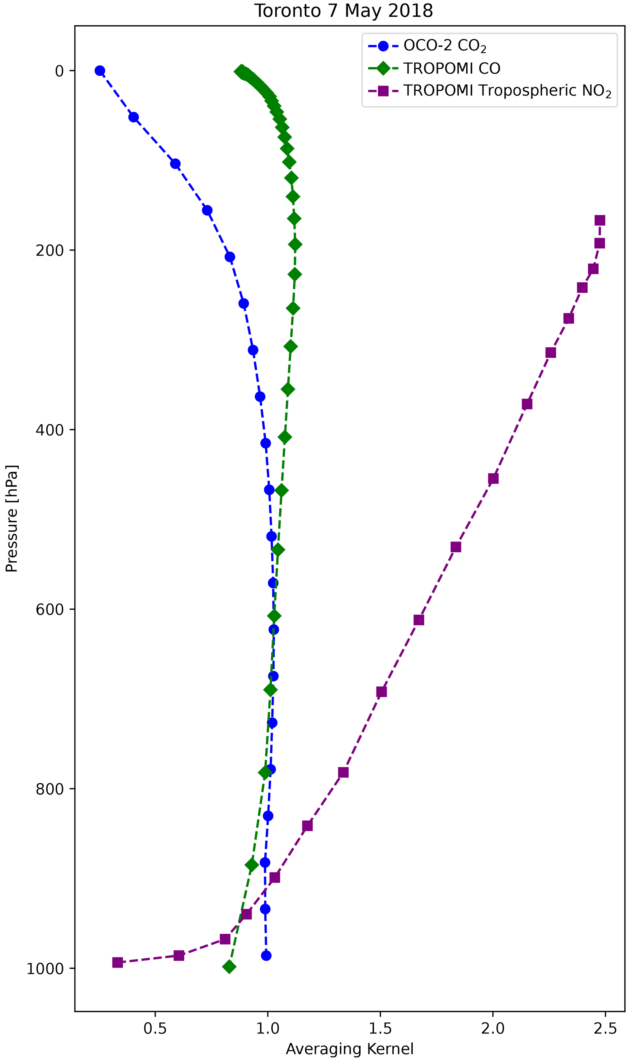
Figure C1 Averaging-kernel profiles for OCO-2 CO₂, TROPOMI CO and TROPOMI NO₂ over Toronto on 7 May 2018.

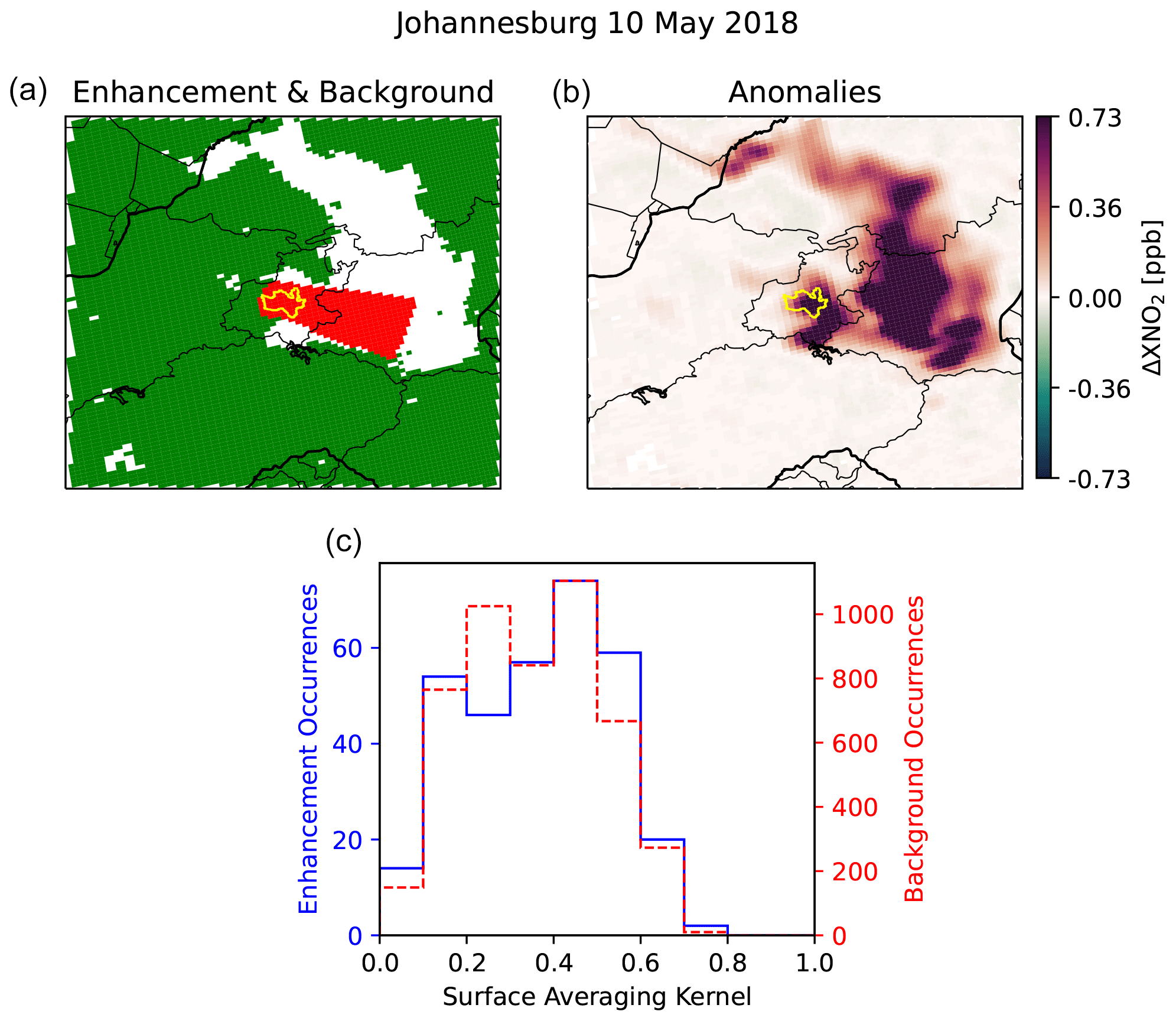
Figure C2 Panel (c) shows the similarity of the distribution of TROPOMI NO₂ surface column averaging-kernel values in the enhancement (solid blue histogram) and in the background (dashed red histogram). The geographical distribution of these surface column averaging kernels are shown in (a), where green points indicate the background region and red points indicate the enhancement region. The solid yellow line outlines the city. Panel (b) shows the NO₂ anomalies in the vicinity of the city.

To isolate the true column difference in Eq. (C5), we need to make an assumption, as it is otherwise intractable. We can assume any combination of the following under the correct conditions:

1. The averaging kernels are the same inside and outside the plume: ${\mathit{a}}_{\mathrm{u}}={\mathit{a}}_{\mathrm{b}}=\mathit{a}$.

2. The priors are the same inside and outside the plume: $c_{\mathrm{u}}^{\mathrm{a}}=c_{\mathrm{b}}^{\mathrm{a}}=c^{\mathrm{a}}$ and ${\mathit{x}}_{\mathrm{u}}^{\mathrm{a}}={\mathit{x}}_{\mathrm{b}}^{\mathrm{a}}={\mathit{x}}^{\mathrm{a}}$.

3. The a priori data are perfect: $c_{\mathrm{u}}^{\mathrm{t}}=c_{\mathrm{u}}^{\mathrm{a}}$, $c_{\mathrm{b}}^{\mathrm{t}}=c_{\mathrm{b}}^{\mathrm{a}}$, ${\mathit{x}}_{\mathrm{u}}^{\mathrm{t}}={\mathit{x}}_{\mathrm{u}}^{\mathrm{a}}$ and ${\mathit{x}}_{\mathrm{b}}^{\mathrm{t}}={\mathit{x}}_{\mathrm{b}}^{\mathrm{a}}$.

If we can reasonably assume that the averaging kernels are the same inside and outside the plume (${\mathit{a}}_{\mathrm{u}}={\mathit{a}}_{\mathrm{b}}=\mathit{a}$), then we can simplify Eq. (C5):

$$\begin{array}{}\text{(C6)}& \begin{array}{rl}\mathrm{\Delta }\widehat{c}& =\mathrm{\Delta }{c}^{\mathrm{a}}+\sum _j\left(a_j{h}_j\right(x_{j\mathrm{u}}^{\mathrm{t}}-x_{j\mathrm{b}}^{\mathrm{t}})-a_j{h}_j(x_{j\mathrm{u}}^{\mathrm{a}}-x_{j\mathrm{b}}^{\mathrm{a}})\\ & =\mathrm{\Delta }{c}^{\mathrm{a}}+\sum _j{a}_j{h}_j(\mathrm{\Delta }{x}_j^{\mathrm{t}}-\mathrm{\Delta }{x}_j^{\mathrm{a}}).\end{array}\end{array}$$

If we can reasonably assume that the priors are the same inside and outside the plume, then Eq. (C5) simplifies but remains intractable:

$$\begin{array}{}\text{(C7)}& \mathrm{\Delta }\widehat{c}=\sum _j\left(a_{j\mathrm{u}}{h}_j{x}_{j\mathrm{u}}^{\mathrm{t}}-a_{j\mathrm{u}}{h}_j{x}_j^{\mathrm{a}}-a_{j\mathrm{b}}{h}_j{x}_j^{\mathrm{t}}+a_{j\mathrm{b}}{h}_j{x}_j^{\mathrm{a}}\right).\end{array}$$

However, if we assume that ${\mathit{a}}_{\mathrm{u}}={\mathit{a}}_{\mathrm{b}}=\mathit{a}$ and ${\mathit{x}}_{\mathrm{u}}^{\mathrm{a}}={\mathit{x}}_{\mathrm{b}}^{\mathrm{a}}={\mathit{x}}^{\mathrm{a}}$, this simplifies further:

$$\begin{array}{}\text{(C8)}& \begin{array}{rl}\mathrm{\Delta }\widehat{c}& =\sum _j\left(a_j{h}_j{x}_{j\mathrm{u}}^{\mathrm{t}}-a_j{h}_j{x}_j^{\mathrm{a}}-a_j{h}_j{x}_{j\mathrm{b}}^{\mathrm{t}}+a_j{h}_j{x}_j^{\mathrm{a}}\right)\\ & =\sum _j{a}_j{h}_j(x_{j\mathrm{u}}^{\mathrm{t}}-x_{j\mathrm{b}}^{\mathrm{t}}).\end{array}\end{array}$$

The equation above is what is often assumed, and rearranging Eq. (C8) to solve for the true enhancement ($\mathrm{\Delta }{c}^{\mathrm{t}}=c_{\mathrm{u}}^{\mathrm{t}}-c_{\mathrm{b}}^{\mathrm{t}}$) gives Eq. (C9), under the assumption that the enhancement is constrained to the surface layer, and therefore $\mathrm{\Delta }{x}_j^{\mathrm{t}}=\mathrm{0}$, $\forall j>\mathrm{1}$. We therefore need only the value of the column averaging kernel at the surface, which we will call a⁰, and we recall that $\sum _j{h}_j{x}_j=c$ to write

$$\begin{array}{}\text{(C9)}& \mathrm{\Delta }{c}^{\mathrm{t}}={\displaystyle \frac{\mathrm{\Delta }\widehat{c}}{a^{\mathrm{0}}}}.\end{array}$$

For the OCO-2 and OCO-3 retrievals, the averaging kernels and a priori profiles inside and outside the plume are negligibly different, and so Eq. (C9) is the correct one to use. For the TROPOMI NO₂ and CO retrievals, we cannot assume that the a priori profiles are the same inside and outside the plume. However, the reported averaging kernels do not differ significantly inside and outside the urban plume, so it is appropriate to use Eq. (C6) under most conditions. (Exceptions to this might be found, for example, in cities with significantly different surface albedo compared with the surrounding region.) Starting with Eq. (C6), again assuming that the enhancements are constrained to the surface layer, we can isolate Δc^t and rearrange:

$$\begin{array}{}\text{(C10)}& \begin{array}{rl}\mathrm{\Delta }\widehat{c}& =\mathrm{\Delta }{c}^{\mathrm{a}}+\sum _j{a}_j{h}_j(\mathrm{\Delta }{x}_j^{\mathrm{t}}-\mathrm{\Delta }{x}_j^{\mathrm{a}})\\ & =\mathrm{\Delta }{c}^{\mathrm{a}}+a^{\mathrm{0}}(\mathrm{\Delta }{c}^{\mathrm{t}}-\mathrm{\Delta }{c}^{\mathrm{a}})\\ \mathrm{\Delta }{c}^{\mathrm{t}}& ={\displaystyle \frac{\mathrm{\Delta }\widehat{c}}{a^{\mathrm{0}}}}-{\displaystyle \frac{(\mathrm{1}-a^{\mathrm{0}})\mathrm{\Delta }{c}^{\mathrm{a}}}{a^{\mathrm{0}}}}.\end{array}\end{array}$$

This equation includes an extra correction term compared with Eq. (C9), which adjusts the measured anomalies by the difference between the urban and rural priors (the prior enhancement), weighted by their contribution to the retrieval (1−a⁰) and divided by the surface pressure averaging kernel. If $c_{\mathrm{u}}^{\mathrm{a}}=c_{\mathrm{b}}^{\mathrm{a}}$, then Eq. (C10) reduces to Eq. (C9).

We include sample averaging-kernel profiles for reference (Fig. C1) and an example of distribution of surface averaging-kernel values in the enhancement/background (Fig. C2).