the Creative Commons Attribution 4.0 License.
the Creative Commons Attribution 4.0 License.
 | 17 Mar 2023
A three-dimensional simulation and process analysis of tropospheric ozone depletion events (ODEs) during the springtime in the Arctic using CMAQ (Community Multiscale Air Quality Modeling System)
Le Cao
Yicheng Gu
Yuhan Luo
The tropospheric ozone depletion event (ODE), first observed at Barrow (now known as Utqiaġvik), Alaska, is a phenomenon that frequently occurs during the springtime in the Arctic. In this study, we performed a three-dimensional model study on ODEs occurring at Barrow and its surrounding areas between 28 March and 6 April 2019 using a 3-D multi-scale air quality model, CMAQ (Community Multiscale Air Quality Modeling System). Several ODEs observed at Barrow were captured, and two of them were thoroughly analyzed using the process analysis method to estimate contributions of horizontal transport, vertical transport, dry deposition, and the overall chemical process to the variations in ozone and bromine species during ODEs. We found that the ODE occurring between 30 and 31 March 2019 (referred to as ODE1) was primarily caused by the horizontal transport of low-ozone air from the Beaufort Sea to Barrow. The formation of this low-ozone air over the sea was largely attributed to a release of sea-salt aerosols from the Bering Strait under strong wind conditions, stemming from a cyclone generated on the Chukotka Peninsula. It was also discovered that the surface ozone dropped to less than 5 ppb over the Beaufort Sea, and the overall chemical process contributed up to 10 ppb to the ozone loss. Moreover, BrO over the sea reached a maximum of approximately 80 ppt. This low-ozone air over the sea was then horizontally transported to Barrow, leading to the occurrence of ODE1. Regarding another ODE on 2 April (ODE2), we found that its occurrence was also dominated by the horizontal transport from the sea, but under the control of an anticyclone. The termination of this ODE was mainly attributed to the replenishment of ozone-rich air from the free troposphere by a strong vertical transport.
- Article
(14219 KB) - Full-text XML
-
Supplement
(39429 KB) - BibTeX
- EndNote


Ozone, one of the most important atmospheric constituents in the atmosphere of the Arctic, has historically attracted much attention from the scientific community. The background level of ozone in the Arctic is approximately 40–60 ppb (parts per billion by volume) (Seinfeld and Pandis, 2016), and the long-range transport of anthropogenic emissions of ozone precursors from North America and East Asia has generally increased the tropospheric ozone in the Arctic since the 1990s (Sharma et al., 2019). However, Oltmans (1981) observed an abnormal decrease in surface ozone at Barrow (now known as Utqiaġvik; 71.3230∘ N, 156.6114∘ W), Alaska, in the springtime. The surface ozone was found to drop from the background level to a few parts per billion within a couple of days or even hours, which is commonly called ozone depletion events (ODEs).
After that, Barrie et al. (1988) found that the tropospheric ODEs are formed due to the occurrence of an auto-catalytic reaction cycle involving bromine chemistry, the major reactions of which are shown below (Barrie et al., 1988; Platt and Hönninger, 2003; von Glasow and Crutzen, 2014):
In this reaction cycle, the total amount of bromine stays constant, which means that the bromine acts as a catalyst for the ozone depletion. Aside from the reaction cycle (Eq. 1), Br and BrO can also react with HO2 radicals, forming HBr and HOBr, respectively. HBr and HOBr are relatively inert, so the formation of these two species tends to terminate the reaction cycle. HBr can also be generated from reactions between Br atoms and olefins or aldehydes, and then it leaves the atmosphere due to its tendency to dissolve (Platt and Hönninger, 2003).
However, heterogeneous reactions taking place at the surface of substrates (such as frost flowers or sea-salt aerosols) lead to the liberation of inert bromine (McConnell et al., 1992; Fan and Jacob, 1992), which is essential for the re-emission of bromine, the so-called “bromine explosion” mechanism (Platt and Lehrer, 1997; Wennberg, 1999). Reaction (R1) represents one of these heterogeneous reactions, which forms active Br2 from bromine ions (Br−):
A similar heterogeneous reaction involving Cl− also occurs:
forming another active bromine species, BrCl. Therefore, additional bromine can be rapidly released into the atmosphere, causing a fast ozone depletion in the boundary layer. Under this condition, the dominant oxidant in the atmosphere shifts from OH, the major product of ozone photolysis, to bromine species. Because the bromine species are capable of accelerating the deposition of mercury from the air, more mercury can enter the ocean and then influence the biosphere through marine wildlife (Simpson et al., 2007; Steffen et al., 2008).
Many researchers have contributed to the study of ODEs. The internal relationship between the ozone depletion and the bromine explosion was established through observations and experiments (Oltmans, 1981; Barrie et al., 1988; Bottenheim et al., 1990; McConnell et al., 1992; Fan and Jacob, 1992; Hausmann and Platt, 1994; Boylan et al., 2014). Furthermore, scientists attempted to reproduce ODEs through parameterizations or model simulations. For example, Lehrer et al. (2004) used a one-dimensional model to identify weather conditions and underlying surface properties necessary for the occurrence of ODEs. They concluded that the sunlight, bromine-containing surface, and strong conversion on the top of the boundary layer are essential conditions for the occurrence of ODEs. These requirements can only be met in the springtime, which is the main reason that ODEs are mostly observed in spring. Thomas et al. (2011, 2012) used a one-dimensional atmospheric boundary layer model named MISTRA-SNOW to study the chemistry on the snow at Summit, Greenland. They concluded that the bromine- and nitrate-containing surfaces help to maintain the concentrations of NO and BrO during the study time.
The first three-dimensional simulation of ODEs was implemented by Zeng et al. (2003, 2006), who found that low surface ozone (<20 ppb) and high BrO were present in about 60 % of the northern high-altitude region. Zeng et al. (2006) also concluded that a strong anti-correlation exists between the tropospheric BrO and the surface temperature. Furthermore, they found that the concentration of BrO is relevant to movements of air masses and the variation in temperature rather than the absolute value of the temperature. Later, by using a global chemistry transport model, p-TOMCAT, Yang et al. (2008, 2010, 2019) proposed that the bromine in polar areas mostly comes from sea-salt aerosols. A release of active bromine into the atmosphere then results in an average of 8 % of the tropospheric ozone loss.
Recently, Herrmann et al. (2021, 2022) and Marelle et al. (2021) tried to reproduce ODEs using a mesoscale forecasting model, WRF-Chem. These studies are a major advancement in 3-D simulations of ODEs. In the study of Herrmann et al. (2021), they concluded that the bromine explosion mechanism alone is unable to maintain enough BrO. Instead, a heterogeneous reaction involving ozone and bromine ions makes the bromine explosion possible. Moreover, Marelle et al. (2021) found that the surface snow and blowing snow are both able to initialize the ODEs. It was also suggested by Marelle et al. (2021) that, although blowing snow is the major source of sea-salt aerosols, it only exerts a weak impact on ODEs. Both studies contribute largely to the 3-D simulations of ODEs.
However, in previous simulations of ODEs, due to the use of self-constructed chemical mechanisms without validations, uncertainties may be induced into chemical simulations. Moreover, contributions of physical and chemical processes to the occurrence of ODEs need to be studied more thoroughly. Therefore, in this study, we conducted simulations of ODEs using a 3-D multi-scale air quality model, CMAQ (Community Multiscale Air Quality Modeling System), focusing on Barrow and the surrounding areas (see Fig. 1a). We used a validated chemical mechanism originally implemented in CMAQ, CB05eh51_ae6_aq, which includes the halogen chemistry (Sarwar et al., 2015; Sherwen et al., 2016; Yarwood et al., 2012). In addition, we performed a process analysis (Gipson, 1999) to estimate the contribution of each physical or chemical process to the variations in ozone and bromine species during ODEs. By doing that, we were able to quantitatively analyze the variations in selected species and evaluate the importance of influencing factors for ODEs.
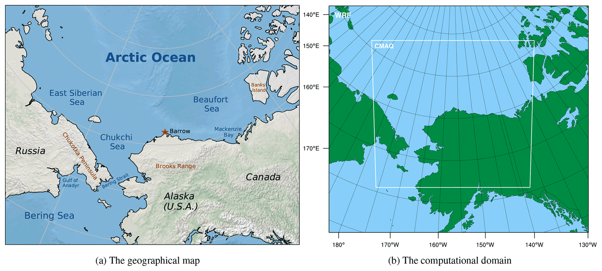
Figure 1The geographical map of the research area and the computational domain used in WRF and CMAQ. The red asterisk in the figure denotes the location of Barrow.
We introduce the configurations of our simulations in Sect. 2 and then present the validations and quantitative analysis of two ODEs in Sect. 3. At last, conclusions and future work are given in Sect. 4.
In this study, the CMAQ model (US EPA Office of Research and Development, 2018) was used to reproduce the ODEs. The WRF model (Weather Research and Forecasting; Skamarock et al., 2008) was used to capture the meteorological parameters and drive the CMAQ model. Hourly measurements of in situ meteorological parameters and ozone were used to validate the simulations.
2.1 Model settings
CMAQ requires the input of meteorological fields including temperature, wind, and pressure to drive the chemical simulations. In this study, outputs of the WRF model were used to drive the CMAQ model.
2.1.1 WRF
The WRF model version 3.9.1, developed by the National Center for Atmospheric Research (NCAR) and National Oceanic and Atmospheric Administration (NOAA), was used to simulate the meteorological fields (Skamarock et al., 2008). The initial conditions and boundary conditions of WRF were given by GDAS/FNL (the Global Data Administration System/Final) re-analysis dataset (National Centers for Environmental Prediction et al., 2015), with a spatial resolution of 0.25∘ × 0.25∘ and a temporal resolution of 6 h. The computational domain used in WRF and CMAQ is shown in Fig. 1b, the center of which is 70.0∘ N, 156.8∘ W. The spatial resolution was set to 9 km. Along the vertical direction, 35 layers were distributed. The time period of the WRF simulation ranges from 25 March to 10 April 2019. The detailed settings of the WRF model are given in Table 1.
Thompson et al. (2008)Janjić (1994)Chen et al. (1997)Janjić (1994)Tiedtke (1989)Iacono et al. (2008)Iacono et al. (2008)Sarwar et al. (2015)Crippa et al. (2020)Buchholz et al. (2019)Mellberg (2014)
2.1.2 CMAQ
In this study, a 3-D regional air quality model, CMAQ, developed by the United States Environmental Protection Agency (EPA), was used to capture the ODEs. CMAQ combines atmospheric science and air quality models together and uses multi-processor technology for three-dimensional simulations of ozone, particulates, and acid deposition (US EPA Office of Research and Development, 2020). In the present study, CMAQ version 5.2.1 (US EPA Office of Research and Development, 2018) was used to capture the variations in ozone and other atmospheric constituents during ODEs. The equation denoting the change in each chemical species in CMAQ is shown below:
In Eq. (2), denotes the temporal change in chemical species. The terms on the right-hand side of Eq. (2) represent advection, diffusion, chemical conversion of species c, emissions of species c, and loss of species c, respectively (US EPA Office of Research and Development, 2018). Equation (2) also covers processes elucidated by the process analysis method adopted in this study, which is presented in a later context. The time period simulated in CMAQ ranges from 28 March to 6 April 2019. More details of the CMAQ configuration can be found in Table 1.
The chemical mechanism originally incorporated in CMAQ, CB05eh51_ae6_aq, was used in this study, and the mechanism includes the halogen chemistry (Sarwar et al., 2015; Sherwen et al., 2016; Yarwood et al., 2012). A complete list of reactions in this mechanism can be found on the website of CMAQ (EPA, 2023). However, the important heterogeneous reaction that determines the bromine explosion mentioned above is still lacking in this mechanism. Thus, we added one reaction into this mechanism:
In Reaction (R3), ASEACAT represents the number concentration of sea-salt aerosols in the model. Based on the study of Mellberg (2014), a reaction coefficient molec.−1 cm3 s−1 was given to Reaction (R3) in the mechanism. This reaction coefficient used in the present study is 10 times larger than that proposed by Mellberg (2014). This is because in the study of Mellberg (2014) bromine concentrations were reported to be underestimated by a factor of 5 to 10 compared to observations. In order to clarify the role of this added heterogeneous reaction, we performed sensitivity tests by altering the rate coefficient of this reaction, which is presented in Sect. 3.4 “Sensitivity tests”.
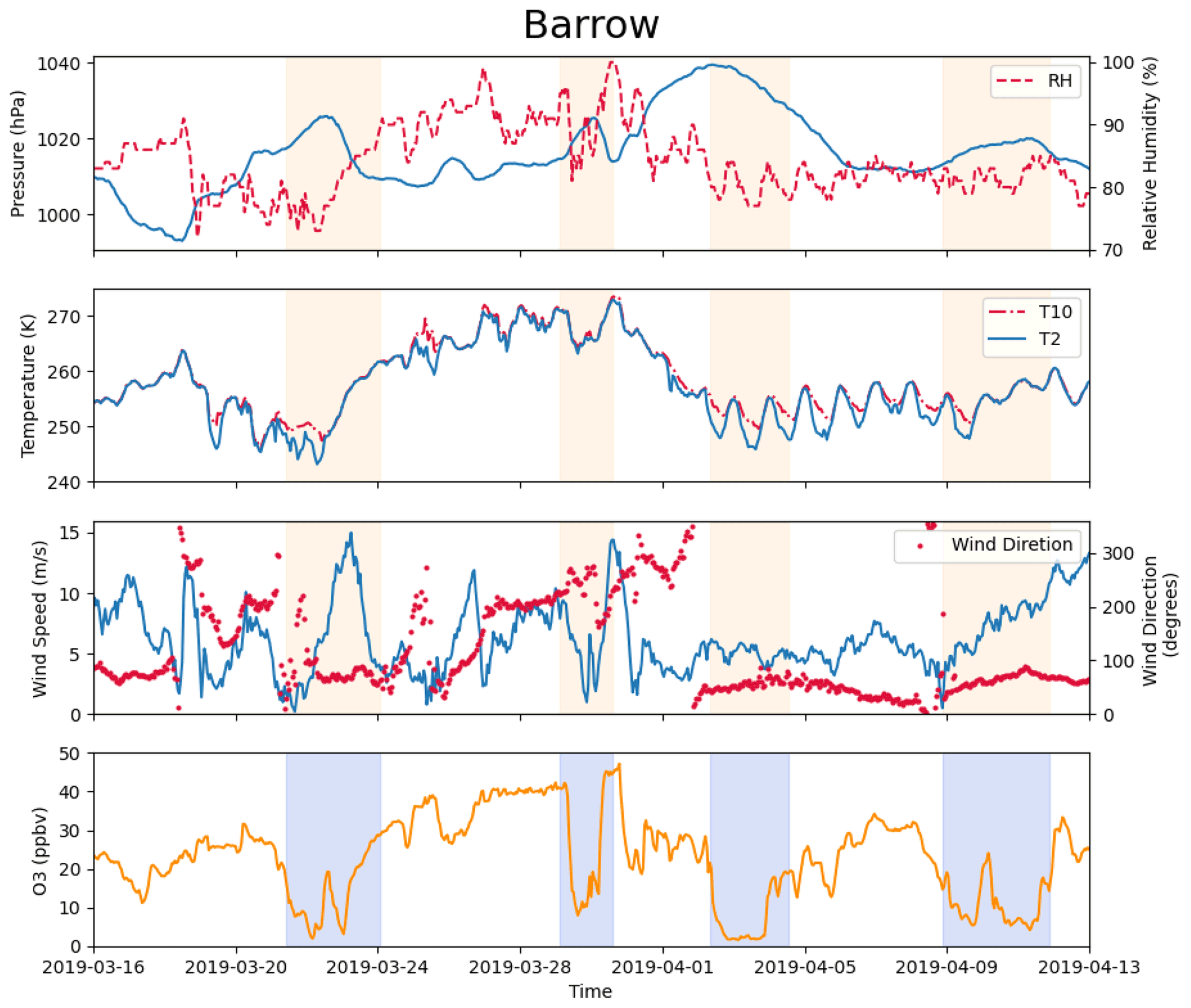
Figure 2Measurements of pressure, relative humidity, temperature at 2 and 10 m, wind direction, wind speed at 10 m, and surface ozone at Barrow (now known as Utqiaġvik) from 16 March to 13 April 2019. The shaded areas denote the occurrence of complete ODEs, the minimum ozone of which is less than 10 ppb.
In addition, we found that in simulations, ozone and other species in the computational domain can be greatly affected by the implemented boundary conditions. Thus, we used a time-dependent boundary condition taken from outputs of an earth system model, the Community Atmosphere Model with Chemistry (CAM-Chem) (Buchholz et al., 2019). However, the chemical mechanism used in CAM-Chem does not consider the influence of the bromine explosion mechanism (Emmons et al., 2020). Therefore, we modified the boundary condition of ozone according to observations (Bottenheim and Chan, 2006). In the study of Bottenheim and Chan (2006), air with low ozone was found to have passed over the Arctic Ocean. Moreover, they found that over the Beaufort Sea and the Chukchi Sea, where the sea ice is frequently formed, the ozone value in the lower troposphere is normally in a range of 0–5.2 ppb. Thus, in the boundary condition of our model, when the air is in the boundary layer and over the sea ice, we set the ozone value to 3 ppb. Meanwhile, in the study of Bottenheim and Chan (2006), the ranges of ozone over the open sea and the coastal area were found to be 5.2–13.85 and 5.2–24.45 ppb, respectively. Thus, in our model, if the air is over the sea, the boundary layer ozone was set to 10 ppb, and if the air is at a coastal area, the boundary layer ozone was set to 15 ppb. In addition, Bottenheim and Chan (2006) also suggested that the free-tropospheric air can be remarkably affected by the bromine explosion, and ODEs can also be influenced by the air transported from the free troposphere. Thus, in the boundary condition of our model, ozone in the free troposphere was also reduced to half of the original value to consider the influence of the bromine explosion. Due to the uncertainty in simulations caused by implementing this modified boundary condition, sensitivity tests were also performed by switching this boundary condition on and off in the CMAQ model, the results of which are presented in Sect. 3.4. The detailed settings of the boundary conditions can also be found in the “Code and data availability” section.
Emissions used in CMAQ were generated by Sparse Matrix Operator Kernel Emissions (SMOKE) developed by EPA (Baek and Seppanen, 2019). EDGAR (Emissions Database for Global Atmospheric Research) version 5.0 was implemented in SMOKE as the emission inventory (Crippa et al., 2018, 2020; Pesaresi et al., 2019; Monforti-Ferrario et al., 2019). A surf zone of 50 m was also set up in the present model due to the existence of ocean in our computational domain. By doing that, more sea spray can be released from the surf zone.
Aside from studying the temporal variations in chemical species, we also used PA, i.e., process analysis (Gipson, 1999), to quantitatively estimate the contribution from each physical or chemical process to the variations in selected air constituents. PA is a module originally included in CMAQ. By performing PA, we were able to analyze the changes in selected species and quantitatively assess the importance of influencing factors. Integrated process rate (IPR) and integrated reaction rate (IRR) were calculated in the PA module. The former includes the net change in species contributed by advection, diffusion, emissions, deposition, and the overall effect of chemical processes. The latter calculates the variation caused by each chemical reaction in the mechanism (Gipson, 1999).
2.2 Measurements
2.2.1 Ground-based observations
The observational data were obtained from the Global Monitoring Laboratory (GML; https://gml.noaa.gov/aftp/data/barrow/, last access: 1 March 2023), which belongs to the National Oceanic and Atmospheric Administration (NOAA). The observational data included surface ozone (McClure-Begley and Oltmans, 2023) and meteorological parameters such as wind direction, wind speed at 10 m, pressure, temperature at 2 and 10 m, and relative humidity (Mefford et al., 1996; Herbert et al., 1986a, b, 1990, 1994). In this study, we focused on the spring of 2019, the measurements of which are shown in Fig. 2. We chose 25 March to 10 April 2019 to simulate. In this time period, several complete ODEs, the minimum ozone of which is less than 10 ppb, are included (see the shaded areas in Fig. 2). Synoptic charts during this period with the surface analysis were also obtained from the Weather Prediction Center, shown in Fig. S1 in the Supplement.
To validate the simulations, we used the Pearson correlation coefficient (R) and the root-mean-square error (RMSE) calculated as follows:
In Eqs. (3) and (4), Si and Oi represent the simulated value and the observed value at the ith time point, respectively. N represents the total number of the time points. and stand for the time-averaged values during this time period. R ranges from −1 to 1. The closer the absolute value of R is to 1, the better the simulations match the observational data. When the value of R is larger than 0.7, it indicates a very strong positive correlation. For RMSE, a smaller RMSE represents less deviation between simulations and observations.
2.2.2 Satellite data
We also compared the tropospheric BrO column density simulated by the model with the satellite data. The simulated tropospheric BrO column density was calculated as follows:
In Eq. (5), ρBrO denotes the column density of the tropospheric BrO (unit: nmol m−2). The right-hand side of Eq. (5) represents an integration of the BrO concentration from the ground to the top of the troposphere, in which p, cBrO, R*, T, and h denote the pressure at this height (unit: Pa), the BrO concentration (unit: ppb), the molar gas constant (unit: ), the temperature (unit: K), and the height (unit: m), respectively. The satellite observations of the tropospheric BrO column density were obtained from EUMETSAT SAF on Atmospheric Composition Monitoring (AC SAF, 2022).
The detailed simulation results are shown in the following section.
In this section, we demonstrate the reliability of the simulations first and then discuss the simulated ODEs in detail. Later, uncertainties in our simulations are illustrated through sensitivity tests by changing the rate of the heterogeneous reaction and switching the implemented boundary condition on and off. At last, a comprehensive process analysis of each ODE is conducted. All geographic names mentioned in the following content can be found in Fig. 1a.
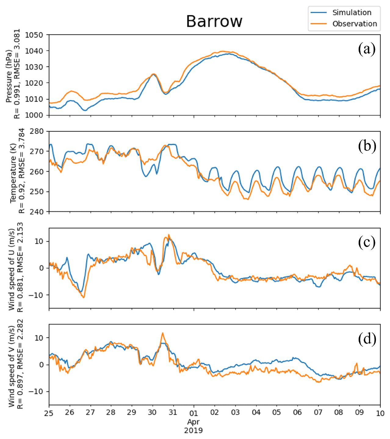
Figure 3Pressure, temperature, and horizontal components of 10 m wind (U and V) obtained from simulations and observations in Barrow from 25 March to 10 April 2019. The correlation coefficient R and the root-mean-square error RMSE are also presented on the vertical axis.
3.1 Validation of the simulations
The temporal variations in meteorological parameters including temperature, horizontal components of the wind speed, and pressure at Barrow simulated by WRF were compared with the observational data, shown in Fig. 3. It can be seen that during this period, the pressure of Barrow (71.3230∘ N, 156.6114∘ W) exhibits a generally increasing trend first, then a decreasing trend, with an abrupt decrease from 30 to 31 March (Fig. 3a). This significant decline in the pressure corresponds to a remarkable change in temperature and horizontal components of wind speed, U and V (see Fig. 3c and d). Values of all the statistical parameters can be found in Table S1 of the Supplement. The correlation coefficients (R) of pressure, temperature, U, and V between simulations and observations are 0.991, 0.920, 0.881, and 0.897, respectively. These correlation coefficients are all very close to 1.0, indicating a high agreement between observations and simulations. The RMSEs of pressure, temperature, U, and V are 3.081 hPa, 3.784 K, 2.153 m s−1, and 2.282 m s−1, respectively. They also denote small deviations between observations and simulations. Thus, we can conclude that the simulated meteorological fields are accurate so that they can be used to drive the chemical simulations of CMAQ during this time period.
The temporal variation in the surface ozone at Barrow simulated by CMAQ was then compared with the observational data, shown in Fig. 4. During this period, the surface ozone at Barrow changed dramatically, and three ODEs were observed.
-
On 29 March, from 07:00 to 16:00 UTC, ozone declined from 41.6 to 9.0 ppb. Then on 30 March from 05:00 to 10:00 UTC, ozone recovered from 13.6 to 45.2 ppb.
-
Later, from 19:00 UTC on 30 March to 04:00 UTC on 31 March, a partial ODE occurred. The surface ozone declined from 47.2 to 19.9 ppb. Then at 10:00 UTC on 31 March, ozone recovered from 18.7 to 32.6 ppb within 3 h.
-
A complete ODE occurred on 2 April. From 05:00 to 22:00 UTC, ozone decreased from 28.4 to 1.8 ppb. After a whole day of low values, ozone recovered from 2.8 to 17.9 ppb.
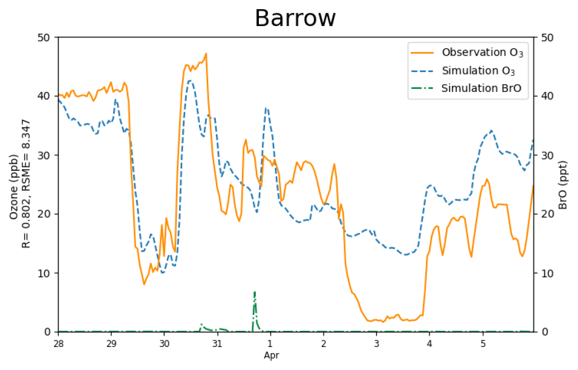
Figure 4The surface ozone (ppb) obtained from simulations and observations together with the simulated BrO at Barrow from 28 March to 5 April 2019. The correlation coefficient R and the root-mean-square error RMSE are also presented on the vertical axis.
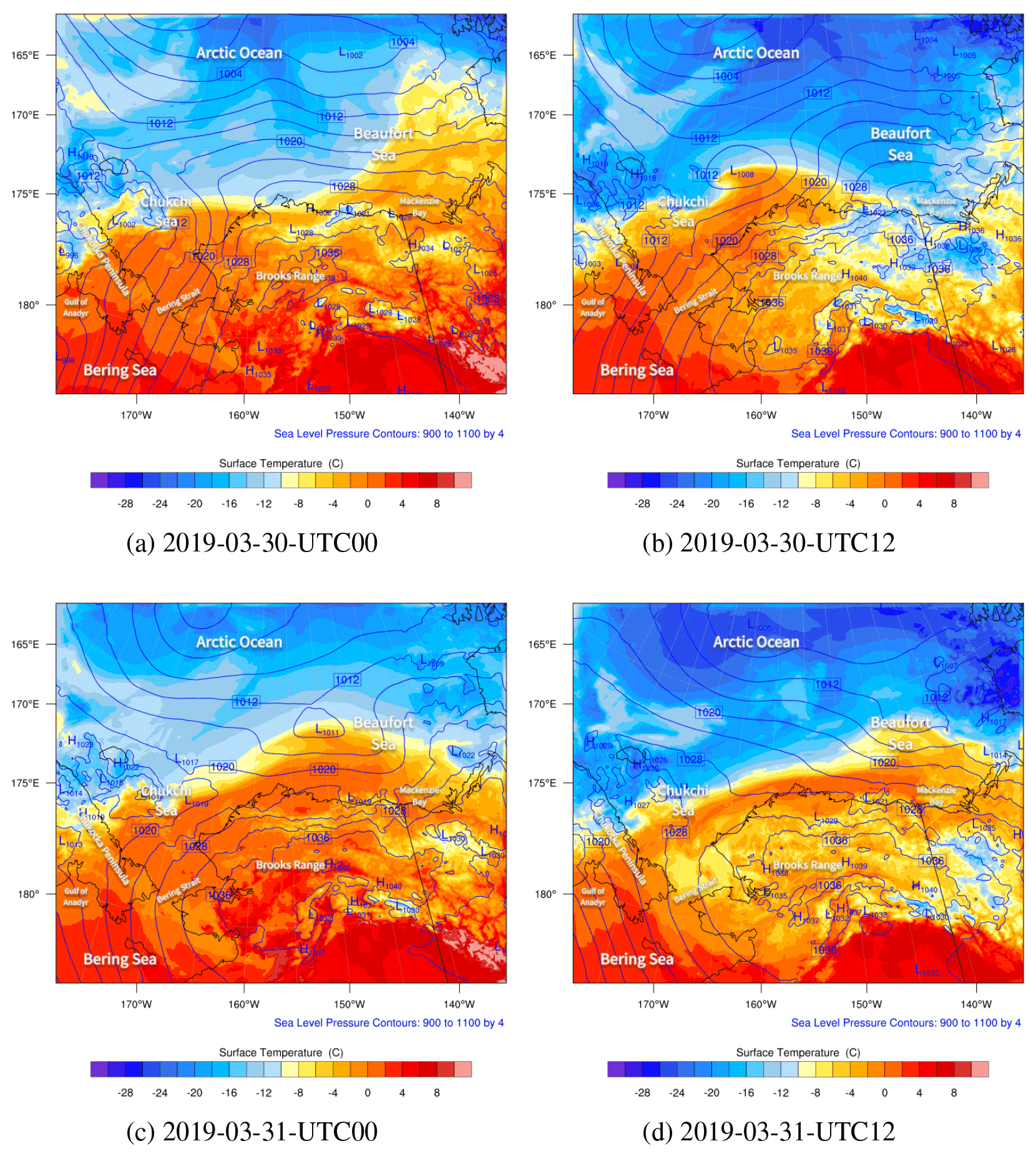
Figure 5The spatial distributions of the sea level pressure (hPa; contour lines) and surface temperature (∘C; contour fills) simulated by WRF from 30 to 31 March 2019.
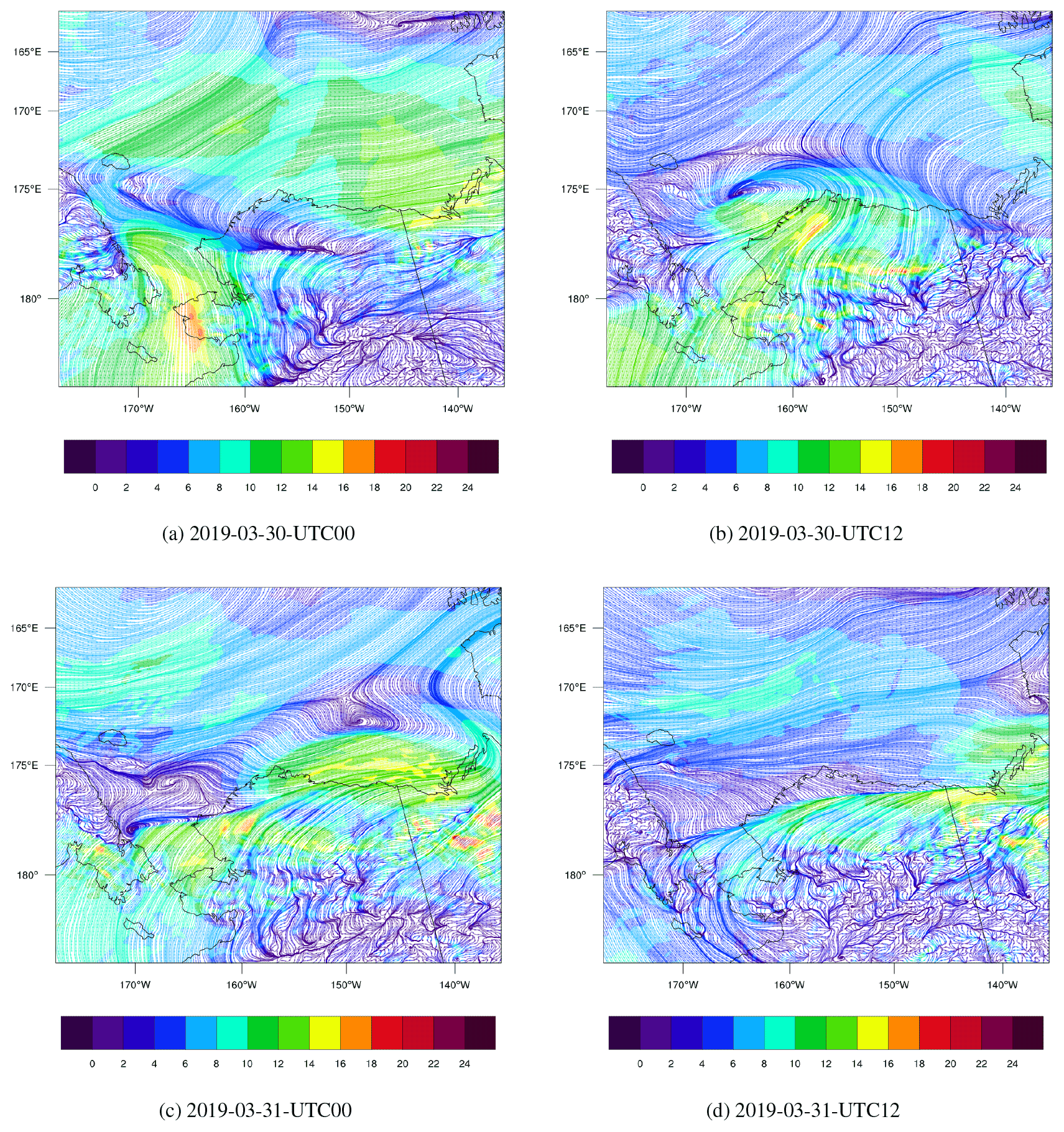
Figure 6The spatial distribution of surface wind (m s−1) and the streamline simulated by WRF from 30 to 31 March 2019.
The correlation coefficient and the root-mean-square error (RMSE) of the surface ozone between the simulations and the observations are 0.802 and 8.347 ppb, respectively. Thus, the variation tendency of the surface ozone was generally reproduced (see Fig. 4), including those dramatic changes discussed above. In particular, not only the start but also the recovery of the ODEs was captured in simulations. However, it should be noted that a fraction of mismatches still exist between simulations and observations. For example, for the complete ODE on 2 April, the model overestimated the surface ozone by approximately 10 ppb. After performing many sensitivity tests (shown in Sect. 3.4), we found this ODE to be greatly contributed by a transport of low-ozone air from the Arctic Ocean, which is located to the north of Barrow. As a result, the simulation of this ODE is heavily influenced by the implemented boundary condition of the model. Although we have modified the boundary condition based on observations, which is described in Sect. 2.1.2, the simulation results still show some deviations from the observations, indicating that improvements of the implemented boundary condition and the adopted chemical mechanism are still needed. Moreover, for the ODE on 29 March, from the satellite measurements (Fig. S2), we found a high BrO level in regions of the Chukchi Sea and the Chukotka Peninsula (66.8∘ N, 176.6∘ W) at 22:44:15 UTC on 28 March 2019 (see Fig. S2a). These high-BrO regions were also found in satellite measurements at the next time point (see Fig. S2b). Because the elevated BrO may reflect a depletion of ozone in these regions, we also modified the boundary condition of our model by reducing the ozone over the Chukotka Peninsula to 40 % of its original value during this time. Simulation results without this modification are shown in Fig. S3. It can be seen that without this modification, the simulated ozone on 29 March would be largely different from observations. More results about the uncertainties caused by the implemented boundary condition are presented and discussed in Sect. 3.4.
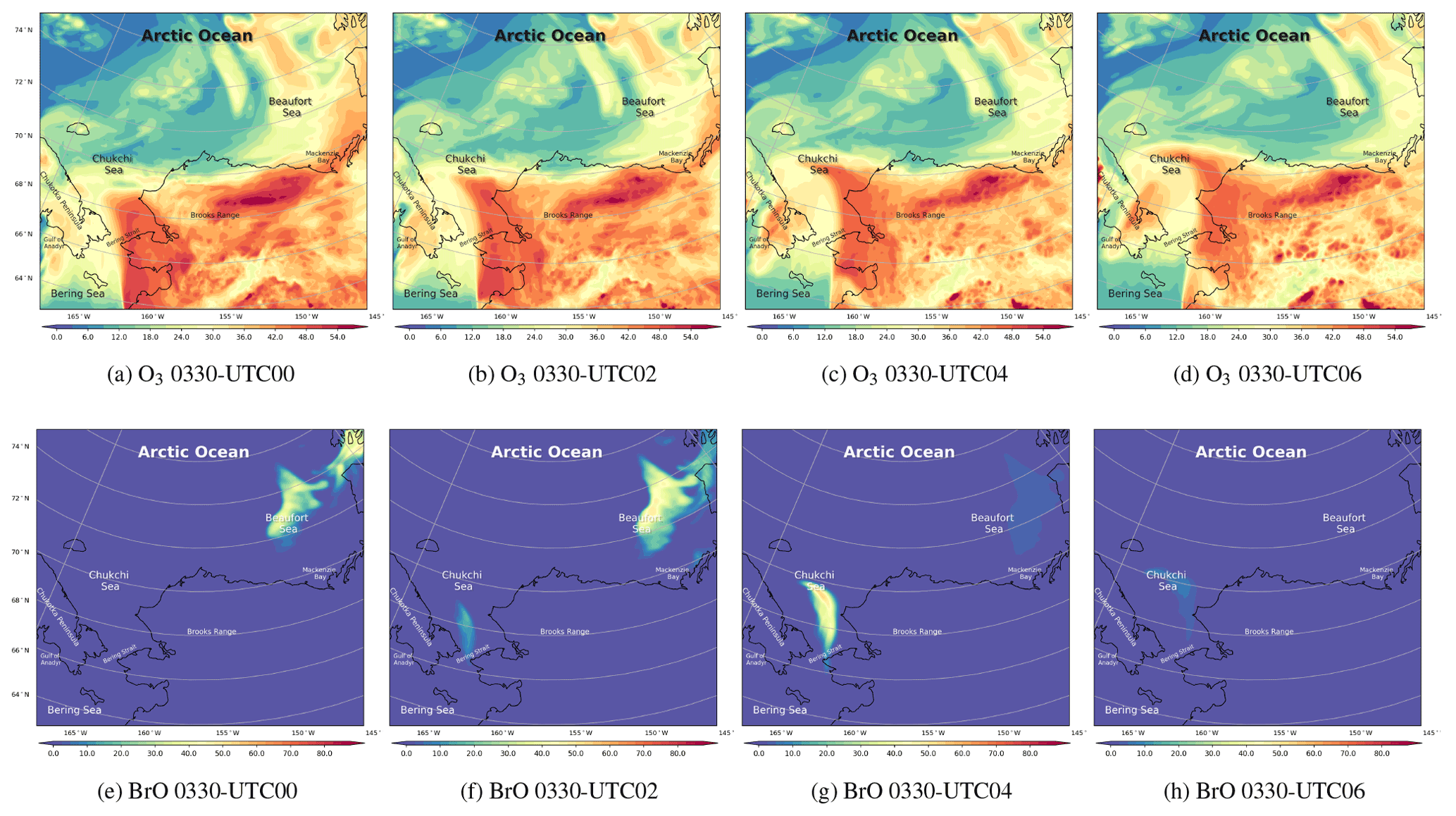
Figure 7The spatial distribution of the surface ozone (ppb) and BrO (ppt) simulated by CMAQ on 30 March 2019.
We also used satellite data to validate our BrO simulations. However, only a qualitative agreement between the simulated BrO and the observations can be achieved. For example, in both simulations and observations, regions with high BrO column density were found to the northwest of Barrow on 30 March (see Fig. S4). Furthermore, in simulations, the maximum of BrO was found to be approximately 2000 nmol m−2, which is similar to the peak value in satellite observations. For a better comparison, improvements to the model, such as adding the iodine chemistry and more heterogeneous reactions, need to be made, which is attributed to a future work.
3.2 Comprehensive analysis of each ODE
In the previous section, we mention that during this period, the pressure of Barrow first exhibits a generally increasing trend, then a decreasing trend, with an abrupt decrease from 30 to 31 March (see Fig. 3a). These meteorological changes at Barrow mainly resulted from two weather conditions, a cyclone and an anticyclone, respectively. Under these circumstances, three ODEs occurred. From our simulations, we found that the ODE on 29 March at Barrow mainly formed by a transport of low-ozone air masses to the west of the Chukchi Sea (71.7∘ N, 169.9∘ W) so that the simulation of this ODE is heavily determined by the applied boundary conditions of the model. Thus, we do not investigate it in more depth in this study. The following two ODEs, occurring on 31 March (named ODE1) and 2 April (named ODE2), are analyzed in detail below.
3.2.1 ODE1 (on 31 March)
The spatial distributions of the surface temperature and the pressure from 30 to 31 March are shown in Fig. 5. Globally, during this period, the Arctic Ocean (79.0∘ N, 156.9∘ W) was dominated by the Arctic vortex, the center pressure of which was low (1002 hPa), and the center temperature was less than −24 ∘C. In contrast, the mainland of Alaska was covered by a uniform pressure field. Figure 5a shows that at 00:00 UTC on 30 March, the gradient of the air temperature on the Beaufort Sea (73.7∘ N, 146.6∘ W) was very large. This large temperature gradient was formed due to the passing-by of a cold front in this area (see Fig. S1b denoting the weather patterns). At the same time, the temperature field around the Chukotka Peninsula became deformed (see Fig. 5a). A low-pressure system (i.e., a cyclone) was also formed over the Chukchi Sea. Then, the low-pressure system developed rapidly and moved northeastward. Meanwhile, the meteorological fields around the cyclone were distorted accordingly, especially the temperature. At 12:00 UTC on 30 March, shown in Fig. 5b, the center of the low-pressure system reached 1008 hPa. This low-pressure system also generated a cold font on the left and a stationary front on the right (see Fig. S1d), leading to a strong temperature gradient around this low pressure. Then, at 00:00 UTC on 31 March (Fig. 5c), the low-pressure system moved to the north of Barrow, and its center pressure increased to 1011 hPa, which indicates a weakening of the low-pressure system. Within a couple of hours (see Fig. 5d), the cyclone continued moving eastward, but a front remained over the sea. For the meteorological field with a finer time interval, please refer to Fig. S5.

Figure 8The spatial distribution of the surface ozone (ppb) and BrO (ppt) simulated by CMAQ from 30 to 31 March.
The spatial distribution of the surface wind from 30 to 31 March is shown in Fig. 6. Figure 6a shows that at 00:00 UTC on 30 March, the wind speed over the Bering Strait (66.0∘ N, 168.9∘ W) was very large; the maximum reached 18 m s-1. With such a high wind speed, sea-salt aerosols can be rapidly released into the atmosphere (shown in Fig. S6b). The liberation of sea-salt aerosols is able to release the reactive bromine into the atmosphere, which can deplete the surface ozone. At 12:00 UTC on 30 March, shown in Fig. 6b, the wind was cyclonic over the Chukchi Sea, and the wind speed was quite large between the two fronts mentioned above. Then, in Fig. 6c, at 00:00 UTC on 31 March the cyclone moved eastward and the wind speed decreased. After 12 h (see Fig. 6d), the wind speed in this area was low. The cyclone moved to the south of Banks Island (73.48∘ N, 121.8∘ W), which indicates the end of this process. For the surface wind with a finer time interval, please refer to Fig. S7. This process is similar to the “bromine cyclone transport event” described by Blechschmidt et al. (2016), but the scale of the process discussed in this study is smaller than that of Blechschmidt et al. (2016).
The spatiotemporal distributions of the simulated ozone and BrO on 30 March are shown in Fig. 7. We mention above that under the high-wind-speed conditions, a large quantity of sea-salt aerosols can be carried into the atmosphere as early as 29 March (see Fig. S6a). However, changes in ozone and BrO were not revealed until 00:00 UTC on 30 March, which means that the response of the chemical field to the change in meteorology is delayed. Figure 7a shows that, over the Arctic Ocean, the surface ozone was at a low level at 00:00 UTC on 30 March. In contrast, over the mainland of Alaska, the surface ozone remained at a background level. BrO is an indicator of ODEs because it increases rapidly during the depletion of ozone. Thus, when ozone near the Chukchi Sea and the Beaufort Sea began to decrease (Fig. 7a and b), the surface BrO started to generate (Fig. 7e and f). In the next 4 h, the surface ozone at the Bering Strait near the Chukchi Sea declined continuously, as shown in Fig. 7c, leading to a strong ozone gradient there. Meanwhile, BrO at this place is explosively generated, shown in Fig. 7g. The maximum of BrO over the Bering Strait was larger than 60 ppt; the high-value areas were consistent with the regions abundant in sea-salt aerosols (Fig. S6). Then, under the control of the strong wind, the air mass with depleted ozone and abundant bromine moved northeastward. Moreover, because of the cyclonic wind discussed above, the air mass containing the depleted ozone and abundant bromine was deformed. At 06:00 UTC on 30 March, the sun was setting. The low-ozone area stopped expanding. The high-BrO area also disappeared due to the absence of Br2 photolysis.
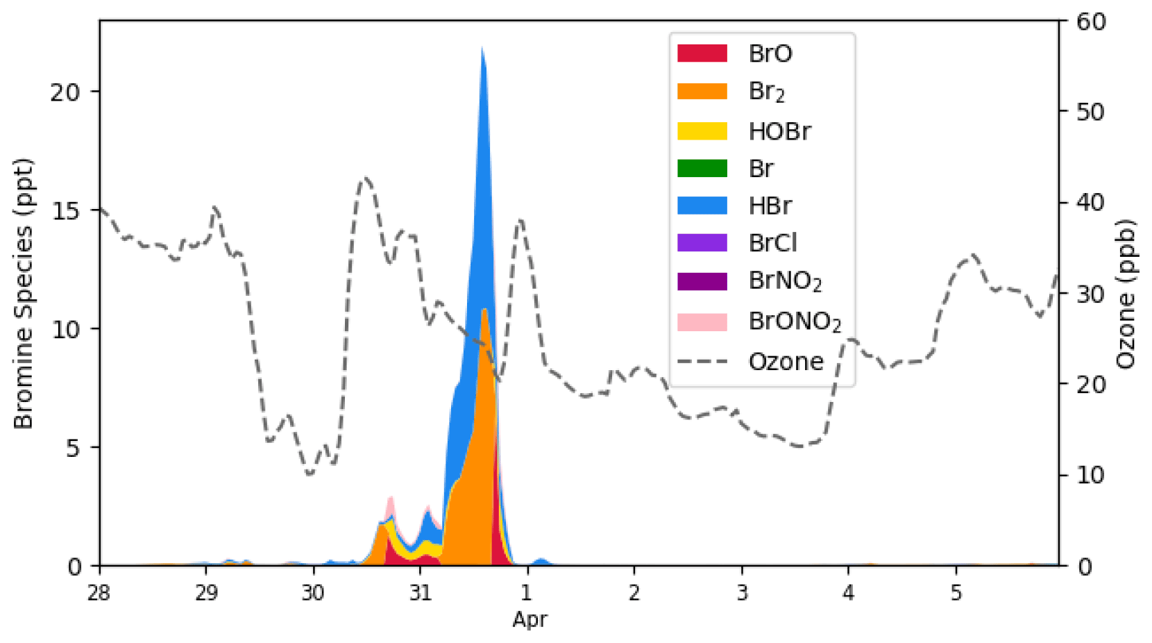
Figure 9The temporal behavior of bromine species (ppt) and ozone (ppb) simulated by CMAQ at Barrow from 28 March to 6 April 2019.
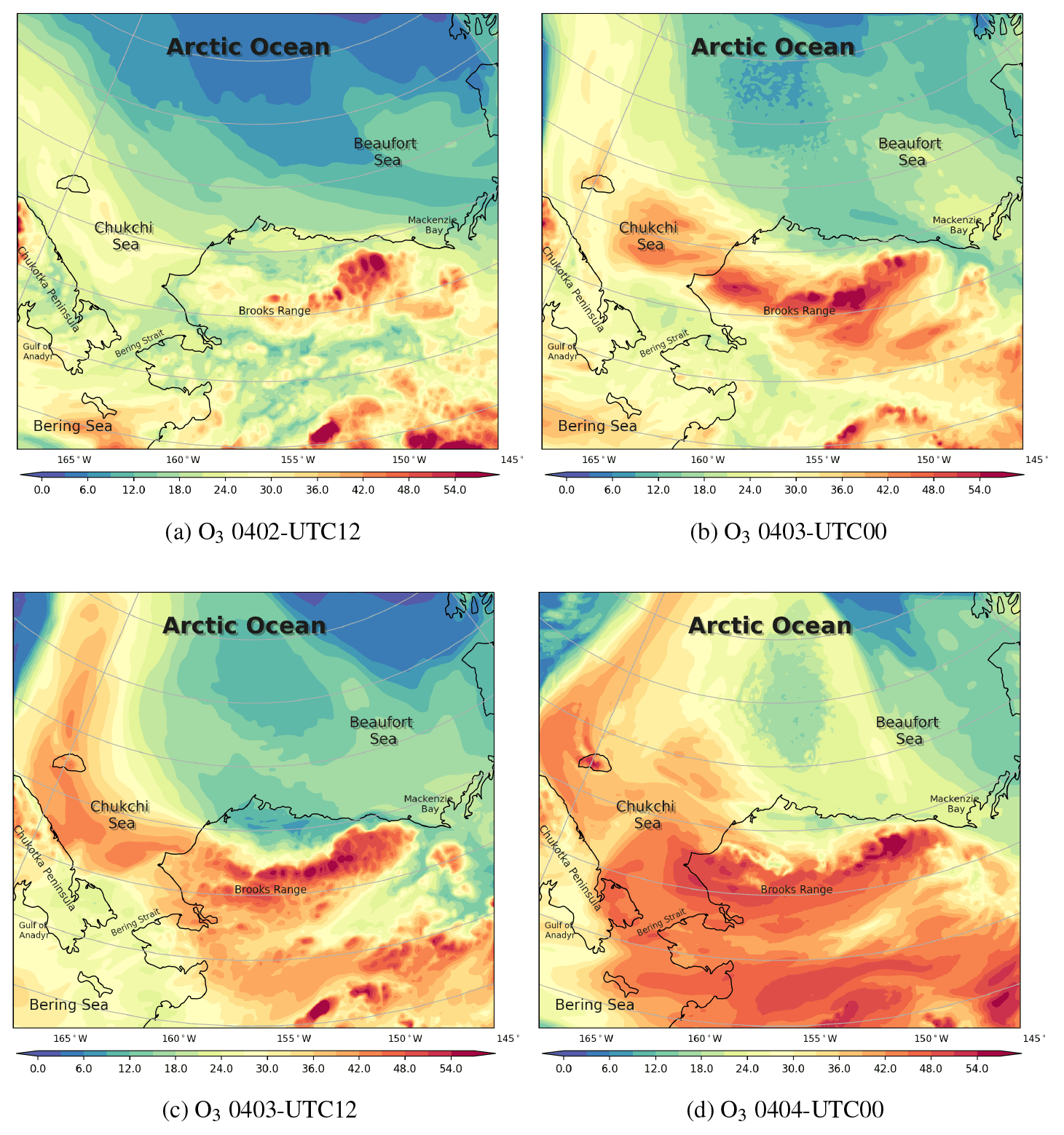
Figure 10The spatial distribution of the surface ozone (ppb) simulated by CMAQ from 2 to 4 April 2019.
The spatiotemporal distributions of the surface ozone and BrO from 30 March to 31 March are also shown in Fig. 8. At 22:00 UTC on 30 March (Fig. 8a), the sun rose again, and the photochemistry started. It can be seen in Fig. 8a and b that the field of ozone was deformed strongly under the control of the cyclonic wind to the north of Barrow. Meanwhile, the reactive bromine returned to the atmosphere due to the bromine explosion mechanism (Fig. 8e). Then at 00:00 and 02:00 UTC on 31 March (see Fig. 8f and g), BrO increased explosively over time. Within 4 h, the surface BrO reached a maximum larger than 80 ppt over the Beaufort Sea, which is consistent with the spatial distribution of sea-salt aerosols (see Fig. S6f and g). Correspondingly, the surface ozone decreased continuously (see Fig. 8c), but the decrease was slightly behind the increase in BrO. At 04:00 UTC on 31 March (see Fig. 8h), the source of BrO was again cut off due to the sunset. In places where the sun set, the level of BrO was significantly lower than that in places where the sun did not set. In contrast, the change in the surface ozone is slightly delayed.
In general, during the time period between 29 and 31 March, the local chemical process, i.e., bromine chemistry, contributed to the partial ODE and the increase in bromine over the Beaufort Sea because of the high-wind conditions and the release of sea-salt aerosols. A maximum of BrO larger than 80 ppt and a minimum of the surface ozone smaller than 15 ppb were found over the sea during this ODE. In contrast, the BrO level observed at Barrow during this time was less than 10 ppt. Thus, we suggested that BrO in the center of the ODE was much larger than that observed at Barrow. Hence, more observations of ozone and bromine over the ocean in the Arctic are required to better understand the properties of ODEs and the bromine explosion mechanism.
The temporal profiles of bromine species and ozone at Barrow in simulations are shown in Fig. 9. We can see that the bromine species, especially Br2, began to increase on 30 March. After sunrise, Br2 photolyzed immediately, releasing two bromine atoms. These bromine atoms then react with the surface ozone and form BrO. Moreover, bromine is continuously released into the atmosphere due to the bromine explosion mechanism. As a result, under this circumstance, ozone began to decrease, while BrO burst into the atmosphere. Meanwhile, as BrO also reacts with HO2 and forms HOBr, the amount of HOBr also increased during this time. When the sun set, due to the absence of Br2 photolysis, BrO declined, while HBr and Br2 accumulated rapidly. The concentration of HBr and Br2 peaked at 10.8 and 11.1 ppt, respectively. Ozone remained at a relatively low level at this time. Then, when the sun rose again, Br2 photolyzed rapidly, and BrO was formed again, reaching a peak of 6.64 ppt in the daytime. Afterwards, the air mass at Barrow was carried eastward; the bromine species at Barrow thus declined, and the ozone recovered.
3.2.2 ODE2 (on 2 April)
Regarding the ODE on 2 April (ODE2), we first focused on the weather conditions. During this time, Barrow and its surrounding areas were occupied by a high-pressure system with a cold center from 2 to 4 April (see surface temperature and pressure in Fig. S8). Under the control of this high-pressure system, a stable stratification with light anticyclonic winds (less than 5 m s−1) was formed in this area. A clear sky, which is a typical weather condition during ODEs (Rancher and Kritz, 1980; Simpson et al., 2007; Anderson and Neff, 2008; Bottenheim et al., 2009; Boylan et al., 2014; Swanson et al., 2020), was also observed. After that, the center of the anticyclone moved slowly southeastward (see Fig. S9 for the surface wind).
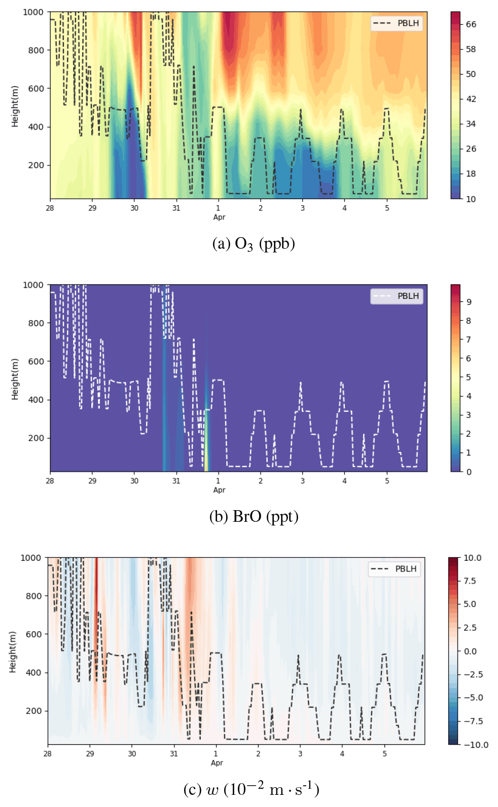
Figure 11Vertical profiles of ozone (ppb), BrO (ppt), and vertical wind speed w (10−2 m s−1) from 28 March to 6 April 2019 at Barrow. The dotted line represents the local planetary boundary layer height (PBLH). A positive w represents an ascending tendency of air parcels, while a negative w denotes a descending tendency of air parcels.
Under this circumstance, ODEs occurred over the Beaufort Sea and Barrow (see Fig. 10). On 2 April, due to the existence of the high-pressure system over the Arctic Ocean (see Fig. 10a), Barrow and its surrounding areas were controlled by a northerly wind so that air masses with low ozone from the Arctic Ocean were transported to Barrow. The situation with a low-level surface ozone at Barrow lasted for about 1 d (Fig. 10b and c). In the study of Bottenheim and Chan (2006), they also found that under the condition of a strong, stable stratification in the Arctic, it may take more time for the surface ozone to recover from the depleted status so that the air parcel with depleted ozone can travel a long distance, such as from the Arctic Ocean to Barrow. Then, the surface ozone of Barrow recovered to the background level, shown in Fig. 10d. It should be noted that some inconsistencies exist between ODE2 simulations and observations. Following many sensitivity tests and the process analysis, which are presented in Sect. 3.4 and 3.5, we conclude that this ODE detected at Barrow was mainly caused by a transport of low-ozone air from the Arctic Ocean, the simulation of which is heavily affected by the implemented boundary condition. In contrast, the recovery of this ODE was mainly caused by a vertical transport of ozone-rich air from the free atmosphere into the boundary layer, which is shown and discussed in a later context. For the variation in the surface ozone with a finer time interval, please refer to Fig. S10.
3.3 Vertical characteristics
The vertical profiles of ozone, BrO, and the vertical wind speed w at Barrow below the height of 1000 m are shown in Fig. 11. As described above, during ODE1, a cyclone formed over the Chukchi Sea and moved northeastward. Thus, at this time stage (on 30 March), the atmospheric activity is intense, and the boundary layer height at Barrow reached 1000 m (see Fig. 11a and b), significantly higher than the typical boundary layer height in the Arctic, 100–500 m (Stull, 1988). Meanwhile, the vertical wind speed w changed dramatically; it was negative in the first half of the day of 30 March (see Fig. 11c). Then in the second half of the day, w became positive. This dramatic change in w indicates a vigorous turbulence in the boundary layer so that BrO can be rapidly mixed aloft (see Fig. 11b). On 31 March, w was mostly positive within the whole 1000 m height. BrO was thus carried outside the boundary layer, leading to the occurrence of the partial ODE1 ubiquitously below the height of 1000 m. Therefore, at this time, the depletion of ozone is not limited within the boundary layer, and the ozone in the free atmosphere can also be influenced.
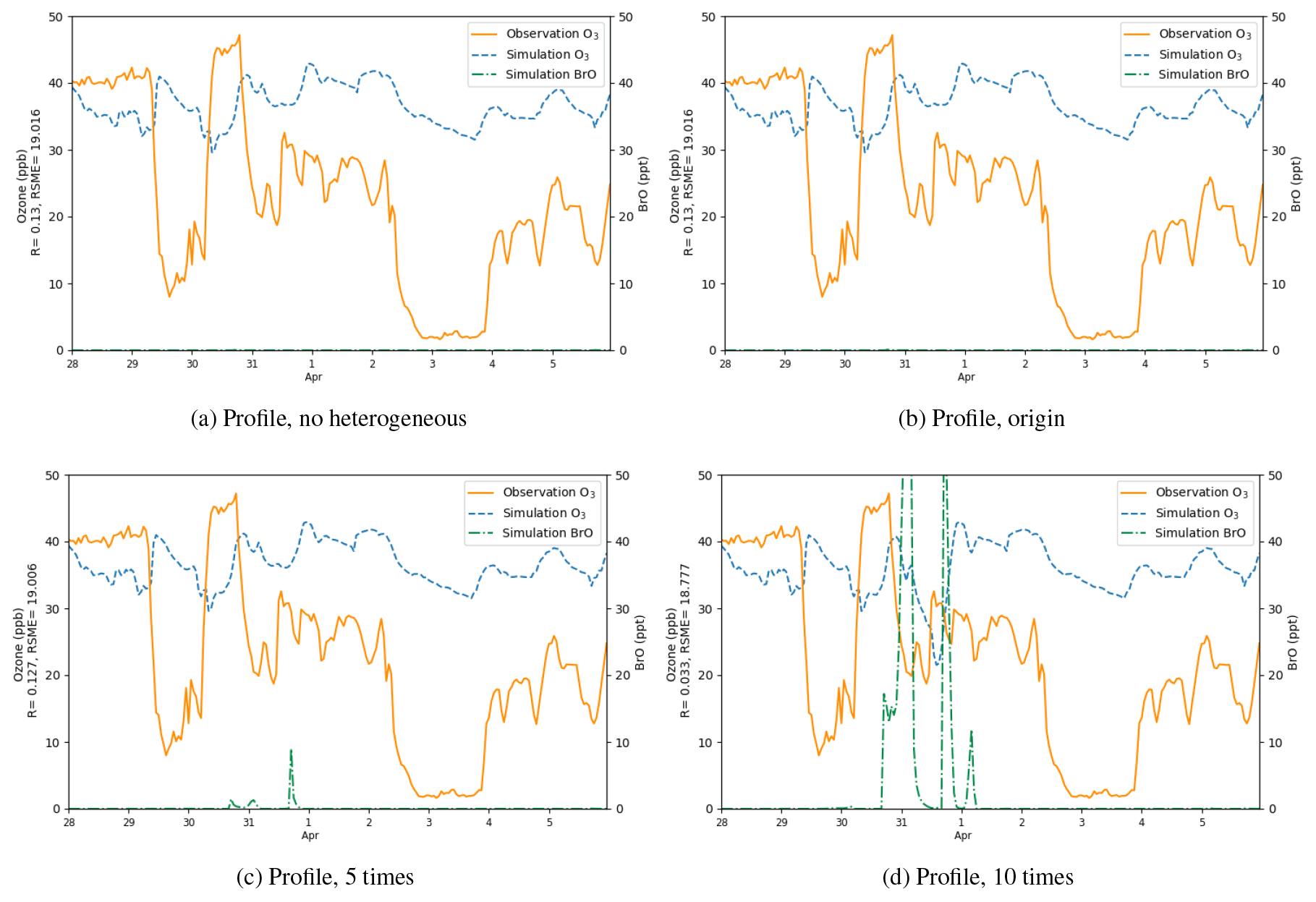
Figure 12Surface ozone (ppb) and BrO (ppt) at Barrow from 28 March to 5 April 2019, obtained from CMAQ simulations using different heterogeneous reaction rates and the default boundary condition, i.e., a static ozone profile. The correlation coefficient R and the root-mean-square error RMSE are also presented on the vertical axis.
With respect to ODE2 during 2–3 April, from the discussions above, Barrow and its surrounding areas were occupied by a high-pressure system. The boundary layer height at Barrow during this time was lower than that in March and shows a distinct diurnal variation (see Fig. 11a). Moreover, ozone shows a strong concentration gradient, especially around the top of the boundary layer (see Fig. 11a). This strong concentration gradient was maintained by the weak vertical diffusion under the stable stratification. In the study of Bottenheim and Chan (2006), they suggested that the stable stratification would inhibit the recovery of the low-ozone status, which corresponded to the case of ODE2. At the end of ODE2, as shown in Fig. 11c, the vertical wind speed was small but negative within these days. As time went by, ozone in the free troposphere was eventually mixed into the boundary layer, and the gradient of ozone was weakened, denoting the end of ODE2.
3.4 Sensitivity tests
Because the present simulations can be greatly affected by the rate of the heterogeneous reaction and the implemented boundary condition (BC), we conducted a series of sensitivity tests and then analyzed the uncertainties induced by these two factors.
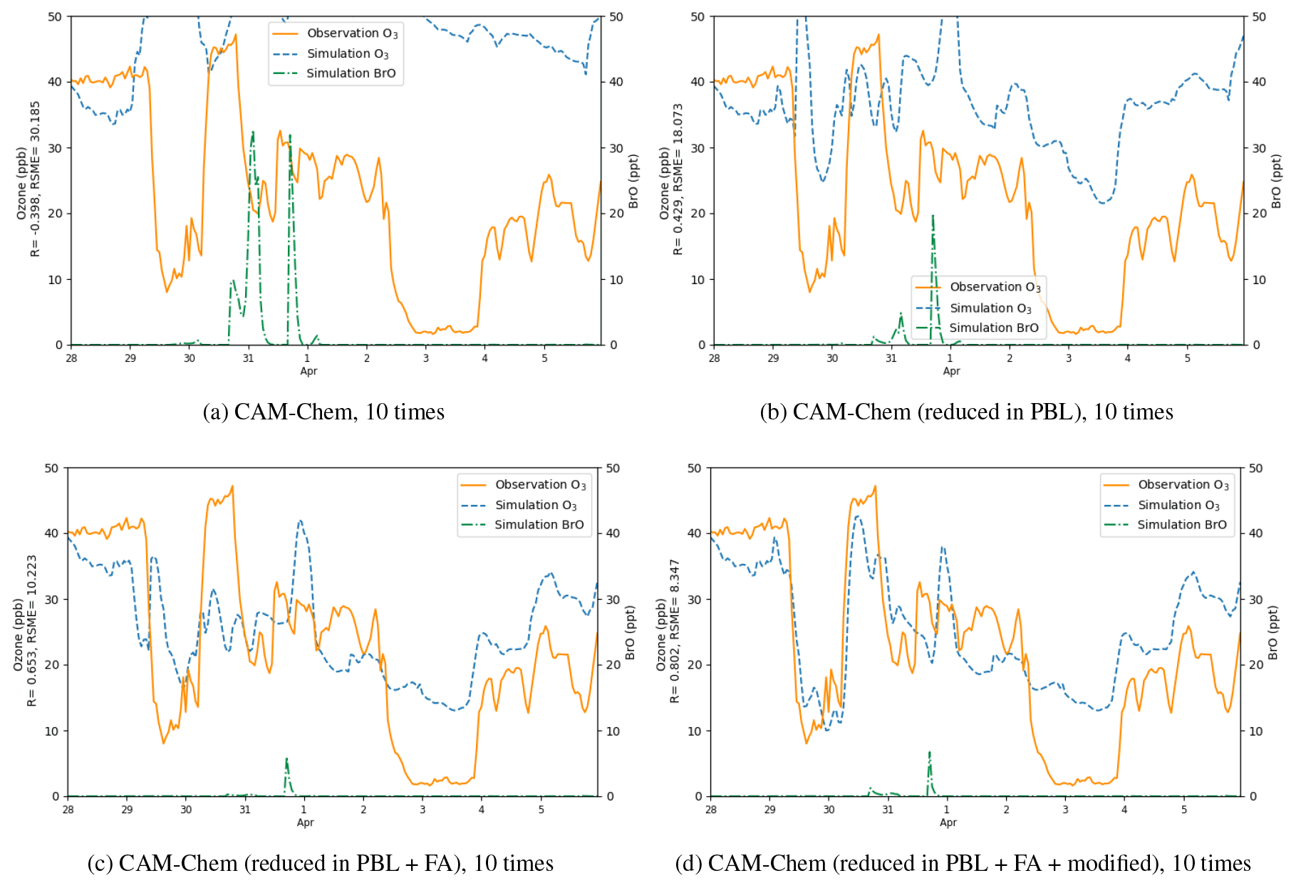
Figure 13Surface ozone (ppb) obtained from simulations and observations together with the simulated BrO at Barrow from 28 March to 5 April 2019. The correlation coefficient R and the root-mean-square error RMSE are also presented on the vertical axis. Simulations were performed using different boundary conditions: (a) time-dependent boundary condition adopted from the outputs of CAM-Chem, (b) outputs of CAM-Chem with a reduction in ozone in the PBL, (c) outputs of CAM-Chem with a reduction in ozone in the PBL and the free atmosphere, (d) outputs of CAM-Chem with a reduction in ozone in the PBL and the free atmosphere as well as a modification of ozone over the Chukotka Peninsula.
Table 2Values of the Pearson correlation coefficient (R) and the root-mean-square error (RMSE; unit: ppb) for the simulated surface ozone at Barrow under different conditions (the heterogeneous reaction rate and boundary conditions). The rate constant of the heterogeneous reaction suggested by Mellberg (2014) was multiplied by 0.0, 1.0, 5.0, and 10.0 and then tested in different simulations. In addition, different boundary conditions (default BC in CMAQ, original CAM-Chem outputs, reduced CAM-Chem outputs but without the modification over the Chukotka Peninsula, reduced and modified CAM-Chem outputs) were also tested.
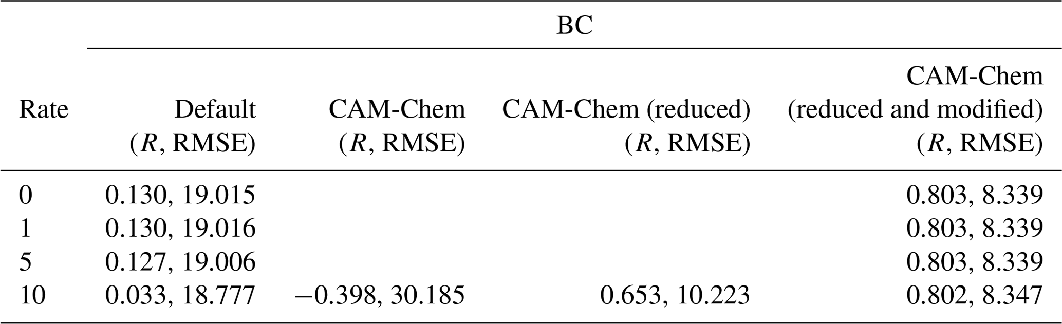
Results of the sensitivity tests in which the heterogeneous reaction rate was altered are shown in Fig. 12. In this series of sensitivity tests, we used the default BC of ozone in CMAQ. This default BC in CMAQ is generated by a static profile, which represents annual average concentrations over the Pacific for the year 2016. This BC reflects conditions in a remote marine environment. From Fig. 12a, we found that with the default BC but without the heterogeneous reaction for the bromine explosion, the simulated ozone did not show any obvious depletion, and the level of BrO was close to zero. Then we added the heterogeneous reaction (Reaction R3) responsible for the bromine explosion into the mechanism with the reaction rate suggested by Mellberg (2014) (Fig. 12b) but found the changes in ozone and BrO to be negligible. Thus, we continued to enlarge the heterogeneous reaction rate. In Fig. 12c, the reaction rate was 5 times larger than that suggested by Mellberg (2014). In this simulation, we found that the BrO level at Barrow elevated to a value range of 0–10 ppt. However, ozone did not show any remarkable change, and the simulated ozone was still higher than the observations. In Fig. 12d, we enlarged the heterogeneous reaction rate to a value that is 10 times that suggested by Mellberg (2014), and we found the ozone during the time period of ODE1 (i.e., 31 March) to decrease to a level similar to observations. Moreover, BrO was also substantially elevated, with a peak higher than 50 ppt. However, ozone concentrations in other time periods were still not significantly influenced by the change in the reaction rate.
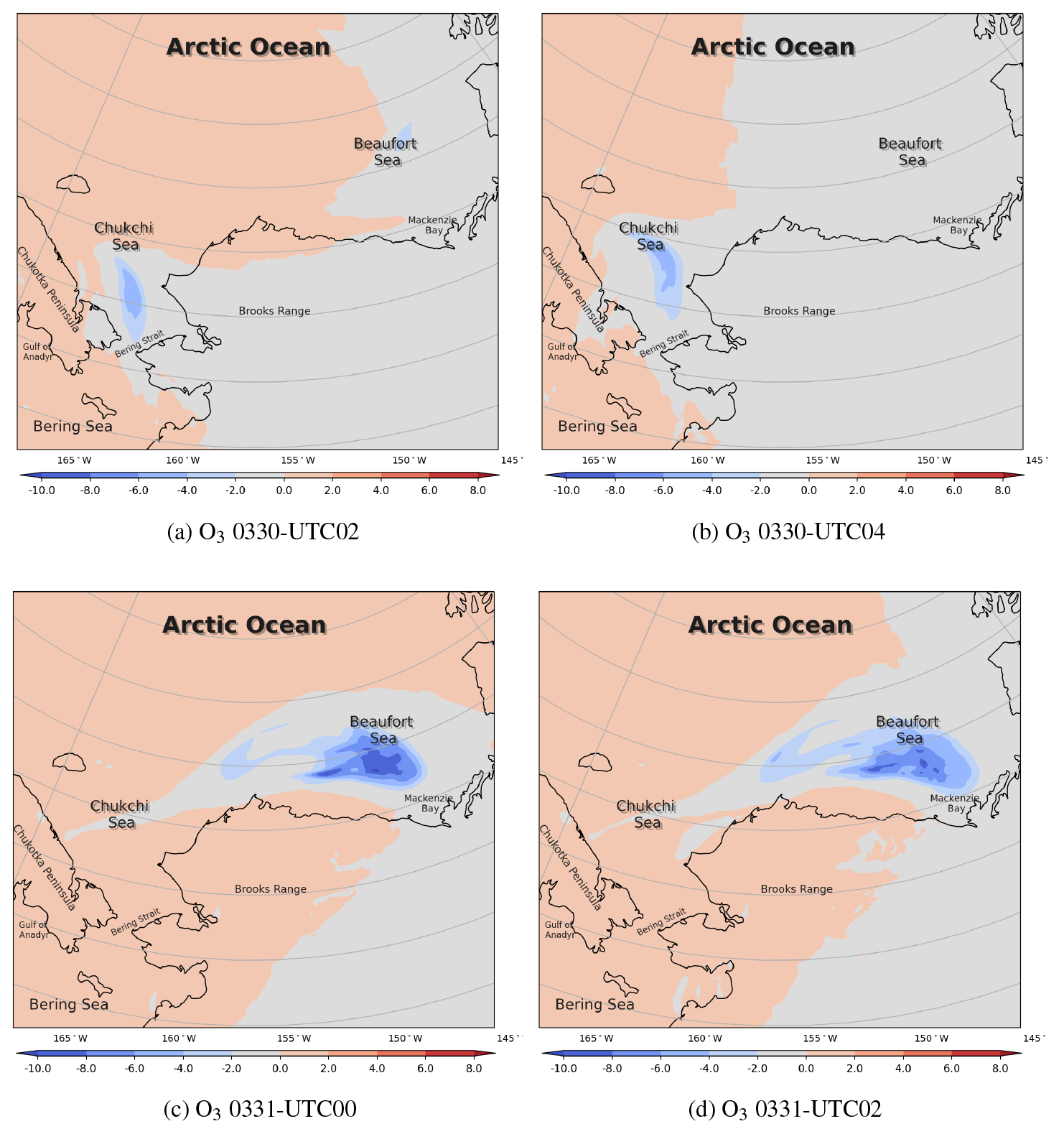
Figure 14The change in surface ozone (ppb) caused by local chemistry, i.e., bromine chemistry, from 30 to 31 March 2019. The positive value represents a chemical production of ozone, while the negative value represents a chemical consumption of ozone.
The statistical parameters for the simulated surface ozone at Barrow using different heterogeneous reaction rates are listed in Table 2. We can see that when the default static BC was used, the correlation coefficients were all close to 0.1. Furthermore, the RMSEs were also large. We also performed a simulation using a reaction rate that is 15 times the rate proposed by Mellberg (2014), and the simulation results even show a negative correlation with the observations. Thus, from this series of sensitivity tests, we concluded that the heterogeneous reaction is only able to affect the simulated ozone and BrO during the time period of ODE1 (i.e., 31 March). For other time periods, other factors such as the implemented boundary condition (BC) might play important roles.

Figure 15The process analysis of surface ozone and bromine species (Br, Br2, BrO, BrCl, HBr, HOBr, BrNO2, and BrONO2) at Barrow from 28 March to 6 April 2019.
Then we tested different boundary conditions in simulations (Fig. 13). We first replaced the default BC with the outputs of the CAM-Chem model (Fig. 13a) but found the simulated ozone to be significantly higher than the observed values. As shown in Table 2, the correlation coefficient for this simulation is negative, and the RMSE reaches 30.185 ppb. The reason for this large deviation might be that the BC of ozone adopted from the CAM-Chem model does not take the influence of the bromine chemistry into account. Thus, we modified the outputs of the CAM-Chem model based on observations (Bottenheim and Chan, 2006) by reducing the ozone in the PBL in the BC according to types of underlying surfaces. Figure 13b shows that after this modification, compared with the previous simulation, the simulated ozone is lower during the whole time period, and the RMSE also decreases. This means that the BC of the model can substantially affect the simulation of ODEs at Barrow. However, the difference between the simulation results and the observations is still moderate. Then we discovered that the ODEs are not only affected by the air in the PBL but also influenced by the air in the free atmosphere. Moreover, ozone in the free atmosphere can also be influenced by the bromine explosion (Bottenheim and Chan, 2006). Thus, we continued to reduce the free-atmospheric ozone in the BC of the model (see Fig. 13c). It was found that the simulated ozone becomes lower than the previous simulation, denoting that the air transported from the free atmosphere also contributed to the ozone decline observed at Barrow. At last, we found that the ozone value over the Chukotka Peninsula in the BC of the model may have a significant impact on the ODE on 29 March. Therefore, we modified the ozone over the Chukotka Peninsula in the BC of the model (see Fig. 13d). As a result, the simulation of the ODE on 29 March becomes more consistent with the observations, especially the termination of this ODE. Thus, we suggested that this ODE at Barrow is highly associated with the air transported from the Chukotka Peninsula.
3.5 Process analysis
In order to study these ODEs in more depth, we then applied the process analysis (PA) to estimate the contribution from each physical or chemical process to the changes in ozone and bromine species. We first show the ozone change during ODE1 caused by the overall chemistry (see Fig. 14). It can be seen that the chemistry forms ozone in the presence of sunlight during the daytime in most areas. However, in places where bromine species were activated, the local chemistry, which is mainly dominated by the bromine chemistry, causes a decrease in ozone. At 02:00 UTC on 30 March, the chemical consumption of surface ozone reached 4 ppb (see Fig. 14a). At 04:00 UTC, when the sun set, the chemical influence disappeared along with the skyline of the sunset (see Fig. 14b). When the sun rose again (Fig. 14c), bromine species began to form again under sunny conditions, and the chemical consumption of the surface ozone reached 10 ppb over the Beaufort Sea. However, this strong consumption lasted only a few hours and declined to 8 ppb at 02:00 UTC, shown in Fig. 14d. For the chemical contribution to the surface ozone with a finer time interval, please refer to Fig. S11.
In contrast to ODE1, the occurrence of ODE2 is not significantly influenced by the local chemistry so that the chemical contribution to the occurrence of ODE2 is negligible. Thus, we do not show it in this paper.
We then calculated the contributions from all the physical and chemical processes to the changes in ozone and bromine species at Barrow from 28 March to 6 April 2019 (Fig. 15). The vertical transport (including vertical diffusion and vertical advection), horizontal transport (including horizontal diffusion and horizontal advection), and dry deposition were contained.
From Fig. 15a, it can be seen that the occurrence of ODE1 at Barrow on 31 March was mainly caused by the horizontal transport, which contributed to approximately 6 ppb of the ozone loss. Thus, we suggest that ozone-depleted air from the ocean was horizontally advected to Barrow, leading to the ozone decline during ODE1. In contrast, the recovery of this ODE on 31 March was attributed to the combined effect of the horizontal transport and the vertical transport, replenishing the boundary layer with ozone-rich air from other areas and the free atmosphere. With respect to ODE2 on 2 April, the ozone loss was also found to be largely contributed by the horizontal transport. A strong vertical transport contributed approximately 7 ppb to the ozone recovery at the end of ODE2 on 3 April, allowing surface ozone to recover to the background level. Thus, vertical transport was primarily responsible for the recovery of ODE2 at Barrow.
Figure 15b shows the contributions of physical and chemical processes to the change in bromine species during the simulated period. On 30 March, it was found that the variations in bromine species were mainly affected by the chemical process, vertical transport, and dry deposition. The chemical process and the vertical transport caused an increase in bromine species by approximately 4 ppt. In contrast, the deposition contributed at most 5 ppt to the bromine loss. This is because during ODE1, the cyclone dominated, leading to a strong wind and a vigorous convection within the boundary layer. As a result, the dry deposition of bromine species was enhanced remarkably. Then, on 31 March, bromine species were horizontally transported to Barrow, contributing approximately 8 ppb to the increase in the total bromine amount. Later, bromine species left Barrow mainly due to the combined effect of the horizontal transport and the vertical transport, which is consistent with the cause of the termination of ODE1 discussed above.
In this study, we conducted a three-dimensional simulation of ozone depletion events (ODEs) over Barrow and its surrounding areas by using a mesoscale air quality model, CMAQ, from 28 March to 6 April 2019. Several ODEs observed at Barrow were captured by the model, and two of them (ODE1 and ODE2) were analyzed thoroughly using process analysis.
During ODE 1, which occurred between 30 and 31 March, a cyclone that moved from the Chukchi Sea to the Beaufort Sea led to strong wind along its trajectory. As a result, a large number of sea-salt aerosols were released from the Bering Strait, liberating active bromine by the bromine explosion mechanism. The bromine-rich air was then carried to the Beaufort Sea with the movement of the cyclone, contributing to a rapid depletion of the surface ozone over the sea. Then, due to the horizontal transport of low-ozone air from the sea, a partial ODE was observed at Barrow. Later, the termination of this ODE was found to be caused by the horizontal advection of ozone-rich air to Barrow and the vertical mixing of the air from layers aloft into the boundary layer. At Barrow on 2 April, ODE2 was found to result from the transport of a low-ozone center from the Arctic Sea to Barrow under the influence of a high-pressure system. This low-ozone status at Barrow then recovered to normal due to the vertical transport of ozone-rich air from the free atmosphere.
From the vertical profiles of ozone, bromine species, and wind during these two ODEs, we found that in the presence of a strong uplift, the low-ozone but bromine-rich air can be carried to an altitude above the top of the boundary layer, which then influenced the air in the free atmosphere. In contrast, when a stable stratification and a temperature inversion occurred, the low-ozone status would last longer and the air containing depleted ozone was able to travel further. However, as time passed by, under the influence of the high-pressure system, the impact of the descending air accumulated so that ozone in the free troposphere was eventually mixed into the boundary layer, ending this ODE.
A process analysis (PA) was also used to quantitatively evaluate the contributions of physical and chemical processes to these two ODEs. It showed that the ODE1 at Barrow was mainly caused by the horizontal transport, which contributed to about 6 ppb of the ozone loss. The recovery of this ODE was largely attributed to the combined effect of the horizontal transport and the vertical transport. In contrast, over the sea, the chemical process significantly contributed to the ozone depletion, reaching 10 ppb at most. The process analysis also showed that the ODE on 2 April (i.e., ODE2) was mainly formed by the horizontal transport. In contrast, at the end stage of ODE2, a strong vertical transport contributed approximately 7 ppb to the ozone recovery so that the ozone recovered to the background level. Thus, the recovery of ODE2 was mainly attributed to the vertical transport.
Although we reproduced the ODEs during the springtime of 2019 and analyzed the contributions of physical and chemical processes to these ODEs, the present study still has some limitations. For instance, the heterogeneous reaction representing the bromine explosion mechanism needs a better parameterization. Moreover, the overestimation of ozone by the model needs further improvements. From the study of Benavent et al. (2022), ozone depletion was suggested to be strongly connected to the enhancement of iodine. Thus, the deviation between simulations and observations in the present simulation may come from the missing iodine chemistry in the chemical mechanism of the model. In the future, we will use a chemical mechanism including a more comprehensive halogen chemistry (i.e., CB6r3m), which has been implemented in CMAQ 5.3 and more recent versions. Furthermore, we would improve the boundary condition used in this study and may also enlarge the computational domain to include more observational sites in the Arctic so that the conclusions reached in this study can be further verified. In addition, more observational data would help to further validate our simulations.
The code of the WRF software was obtained from https://www2.mmm.ucar.edu/wrf/users/download/get_sources.html (last access: 9 March 2023; WRF, 2023). The code of the CMAQ software was taken from https://github.com/USEPA/CMAQ/ (last access: 9 March 2023; USEPA, 2023). The FNL data were adopted from https://doi.org/10.5065/D65Q4T4Z. Outputs of CAM-Chem model for the implemented boundary conditions of CMAQ were obtained from https://www.acom.ucar.edu/cam-chem/cam-chem.shtml (last access: 9 March 2023; Buchholz et al., 2019). The observational data of in situ meteorology and ozone were provided by the Global Monitoring Laboratory (GML) (https://gml.noaa.gov/aftp/data/barrow/, last access: 9 March 2023; NOAA, 2023), belonging to the National Oceanic and Atmospheric Administration (NOAA). The GOME-2 satellite data of the tropospheric BrO column density were taken from https://navigator.eumetsat.int/product/EO:EUM:DAT:0604 (last access: 9 March 2023; AC SAF, 2022). The surface analysis was obtained from Weather Prediction Center (http://www.wpc.ncep.noaa.gov/html/sfc-zoom.php, last access: 9 March 2023; WPC, 2023). The code for changing the boundary conditions of CMAQ can be found in https://github.com/Simeng-unique/acp-supplements (last access: 9 March 2023; Simeng-unique, 2023).
The Video supplement related to this article can be found at https://github.com/Simeng-unique/acp-supplements.
The supplement related to this article is available online at: https://doi.org/10.5194/acp-23-3363-2023-supplement.
LC conceived the idea of the article and extensively revised the manuscript. SL configured and performed the computations. SL also revised the chemical mechanisms and wrote the paper together with LC. YG and YL participated in discussions and gave valuable suggestions on the improvement of the manuscript. All the authors listed read and approved the final paper.
The authors declare that they have no conflict of interest.
Publisher’s note: Copernicus Publications remains neutral with regard to jurisdictional claims in published maps and institutional affiliations.
Numerical calculations in this paper have been performed on the high-performance computing system at the High Performance Computing Center, Nanjing University of Information Science and Technology. The authors would also like to sincerely thank Barron Henderson and Golam Sarwar from the US EPA for helping us deal with the ocean file, which is to be used in a future study using CMAQ v5.3.2.
This research has been supported by the National Key Research and Development Program of China (grant no. 2022YFC3701204) and the National Natural Science Foundation of China (grant no. 41705103).
This paper was edited by Jens-Uwe Grooß and reviewed by Anoop Mahajan and one anonymous referee.
AC SAF: GOME-2 Tropospheric BrO Column Data Record Release 1 – Metop, EUMETSAT [data set], https://doi.org/10.15770/EUM_SAF_O3M_0012, 2022. a, b
Anderson, P. S. and Neff, W. D.: Boundary layer physics over snow and ice, Atmos. Chem. Phys., 8, 3563–3582, https://doi.org/10.5194/acp-8-3563-2008, 2008. a
Baek, B. and Seppanen, C.: CEMPD/SMOKE: SMOKE v4.7 Public Release, Zenodo, (October 2019), https://doi.org/10.5281/zenodo.3476744, 2019. a
Barrie, L. A., Bottenheim, J. W., Schnell, R. C., Crutzen, P. J., and Rasmussen, R. A.: Ozone destruction and photochemical reactions at polar sunrise in the lower Arctic atmosphere, Nature, 334, 138–141, https://doi.org/10.1038/334138a0, 1988. a, b, c
Benavent, N., Mahajan, A. S., Li, Q., Cuevas, C. A., Schmale, J., Angot, H., Jokinen, T., Quéléver, L. L. J., Blechschmidt, A. M., Zilker, B., Richter, A., Serna, J. A., Garcia-Nieto, D., Fernandez, R. P., Skov, H., Dumitrascu, A., oes Pereira, P. S., Abrahamsson, K., Bucci, S., Duetsch, M., Stohl, A., Beck, I., Laurila, T., Blomquist, B., Howard, D., Archer, S. D., Bariteau, L., Helmig, D., Hueber, J., Jacobi, H.-W., Posman, K., Dada, L., Daellenbach, K. R., and Saiz-Lopez, A.: Substantial contribution of iodine to Arctic ozone destruction, Nat. Geosci., 15, 770–773, https://doi.org/10.1038/s41561-022-01018-w, 2022. a
Blechschmidt, A.-M., Richter, A., Burrows, J. P., Kaleschke, L., Strong, K., Theys, N., Weber, M., Zhao, X., and Zien, A.: An exemplary case of a bromine explosion event linked to cyclone development in the Arctic, Atmos. Chem. Phys., 16, 1773–1788, https://doi.org/10.5194/acp-16-1773-2016, 2016. a, b
Bottenheim, J. W. and Chan, E.: A trajectory study into the origin of spring time Arctic boundary layer ozone depletion, J. Geophys. Res.-Atmos., 111, D19301, https://doi.org/10.1029/2006JD007055, 2006. a, b, c, d, e, f, g, h
Bottenheim, J. W., Barrie, L. A., Atlas, E., Heidt, L. E., Niki, H., Rasmussen, R. A., and Shepson, P. B.: Depletion of lower tropospheric ozone during Arctic spring: The Polar Sunrise Experiment 1988, J. Geophys. Res.-Atmos., 95, 18555–18568, https://doi.org/10.1029/JD095iD11p18555, 1990. a
Bottenheim, J. W., Netcheva, S., Morin, S., and Nghiem, S. V.: Ozone in the boundary layer air over the Arctic Ocean: measurements during the TARA transpolar drift 2006–2008, Atmos. Chem. Phys., 9, 4545–4557, https://doi.org/10.5194/acp-9-4545-2009, 2009. a
Boylan, P., Helmig, D., Staebler, R., Turnipseed, A., Fairall, C., and Neff, W.: Boundary layer dynamics during the Ocean-Atmosphere-Sea-Ice-Snow (OASIS) 2009 experiment at Barrow, AK, J. Geophys. Res.-Atmos., 119, 2261–2278, https://doi.org/10.1002/2013JD020299, 2014. a, b
Buchholz, R. R., Emmon, L. K., Tilmes, S., and The CESM2 Development Team: CESM2.1/CAM-chem Instantaneous Output for Boundary Conditions, Tech. rep., UCAR/NCAR – Atmospheric Chemistry Observations and Modeling Laboratory, https://doi.org/10.5065/NMP7-EP60, subset used Lat: 20 to 88, Lon: −180 to −130, March–April, NCAR UCAR [data set], https://www.acom.ucar.edu/cam-chem/cam-chem.shtml (last access: 9 March 2023), 2019. a, b, c
Chen, F., Janjić, Z., and Mitchell, K.: Impact of Atmospheric Surface-layer Parameterizations in the new Land-surface Scheme of the NCEP Mesoscale Eta Model, Bound.-Lay. Meteorol., 85, 391–421, https://doi.org/10.1023/A:1000531001463, 1997. a
Crippa, M., Guizzardi, D., Muntean, M., Schaaf, E., Dentener, F., van Aardenne, J. A., Monni, S., Doering, U., Olivier, J. G. J., Pagliari, V., and Janssens-Maenhout, G.: Gridded emissions of air pollutants for the period 1970–2012 within EDGAR v4.3.2, Earth Syst. Sci. Data, 10, 1987–2013, https://doi.org/10.5194/essd-10-1987-2018, 2018. a
Crippa, M., Solazzo, E., Huang, G., Guizzardi, D., Koffi, E., Muntean, M., Schieberle, C., Friedrich, R., and Janssens-Maenhout, G.: High resolution temporal profiles in the Emissions Database for Global Atmospheric Research, Sci. Data, 7, 121, https://doi.org/10.1038/s41597-020-0462-2, 2020. a, b
Emmons, L. K., Schwantes, R. H., Orlando, J. J., Tyndall, G., Kinnison, D., Lamarque, J.-F., Marsh, D., Mills, M. J., Tilmes, S., Bardeen, C., Buchholz, R. R., Conley, A., Gettelman, A., Garcia, R., Simpson, I., Blake, D. R., Meinardi, S., and Pétron, G.: The Chemistry Mechanism in the Community Earth System Model Version 2 (CESM2), J. Adv. Model. Earth Syst., 12, e2019MS001882, https://doi.org/10.1029/2019MS001882, 2020. a
EPA: Code base for the U.S. EPA's Community Multiscale Air Quality Model (CMAQ), Tech. rep., EPA, https://github.com/USEPA/CMAQ/blob/5.2.1/CCTM/src/MECHS/cb05eh51_ae6_aq/mech_cb05eh51_ae6_aq.def (last access: 9 March 2023), 2023. a
Fan, S.-M. and Jacob, D.: Surface ozone depletion in Arctic spring sustained by bromine reactions on aerosols, Nature, 359, 522–524, https://doi.org/10.1038/359522a0, 1992. a, b
Gipson, G. L.: Chapter 16: Process analysis, Science Algorithms of the EPA Models-3 Community Multiscale Air Quality (CMAQ) Modeling System, https://nepis.epa.gov/Exe/ZyPURL.cgi?Dockey=30003R9Y.txt (last access: 9 March 2023), ePA/600/R-99/030, 1999. a, b, c
Hausmann, M. and Platt, U.: Spectroscopic measurement of bromine oxide and ozone in the high Arctic during Polar Sunrise Experiment 1992, J. Geophys. Res.-Atmos., 99, 25399–25413, https://doi.org/10.1029/94JD01314, 1994. a
Herbert, G., Green, E., Harris, J., Koenig, G., Roughton, S., and Thaut, K.: Control and Monitoring Instrumentation for the Continuous Measurement of Atmospheric CO2 and Meteorological Variables, J. Atmos. Ocean. Technol., 3, 414–421, 1986a. a
Herbert, G., Green, E., Koenig, G., and Thaut, K.: Monitoring instrumentation for the continuous measurement and quality assurance of meteorological observations, Tech. rep., NOAA Tech. Memo. ERL ARL-148, Environmental Research Laboratories (U.S.), 1986b. a
Herbert, G., Harris, J., Bieniulis, M., and McCutcheon, J.: Acquisition and Data Management, in CMDL Summary Report 1989, Tech. Rep. 18, 50 pp., https://gml.noaa.gov/publications/summary_reports/summary_report_18.pdf (last access: 14 March 2013), 1990. a
Herbert, G., Bieniulis, M., Mefford, T., and Thaut, K.: Acquisition and Data Management Division, in CMDL Summary Report 1993, Tech. Rep. 22, https://gml.noaa.gov/publications/summary_reports/summary_report_22.pdf (last access: 14 March 2013), 1994. a
Herrmann, M., Sihler, H., Frieß, U., Wagner, T., Platt, U., and Gutheil, E.: Time-dependent 3D simulations of tropospheric ozone depletion events in the Arctic spring using the Weather Research and Forecasting model coupled with Chemistry (WRF-Chem), Atmos. Chem. Phys., 21, 7611–7638, https://doi.org/10.5194/acp-21-7611-2021, 2021. a, b
Herrmann, M., Schöne, M., Borger, C., Warnach, S., Wagner, T., Platt, U., and Gutheil, E.: Ozone depletion events in the Arctic spring of 2019: a new modeling approach to bromine emissions, Atmos. Chem. Phys., 22, 13495–13526, https://doi.org/10.5194/acp-22-13495-2022, 2022. a
Iacono, M. J., Delamere, J. S., Mlawer, E. J., Shephard, M. W., Clough, S. A., and Collins, W. D.: Radiative forcing by long-lived greenhouse gases: Calculations with the AER radiative transfer models, J. Geophys. Res.-Atmos., 113, D13103, https://doi.org/10.1029/2008JD009944, 2008. a, b
Janjić, Z. I.: The Step-Mountain Eta Coordinate Model: Further Developments of the Convection, Viscous Sublayer Turbulence Closure Schemes, Mon. Weather Rev., 122, 927–945, https://doi.org/10.1175/1520-0493(1994)122<0927:TSMECM>2.0.CO;2, 1994. a, b
Lehrer, E., Hönninger, G., and Platt, U.: A one dimensional model study of the mechanism of halogen liberation and vertical transport in the polar troposphere, Atmos. Chem. Phys., 4, 2427–2440, https://doi.org/10.5194/acp-4-2427-2004, 2004. a
Marelle, L., Thomas, J. L., Ahmed, S., Tuite, K., Stutz, J., Dommergue, A., Simpson, W. R., Frey, M. M., and Baladima, F.: Implementation and Impacts of Surface and Blowing Snow Sources of Arctic Bromine Activation Within WRF-Chem 4.1.1, J. Adv. Model. Earth Syst., 13, e2020MS002391, https://doi.org/10.1029/2020MS002391, 2021. a, b, c
McClure-Begley, A. and Oltmans. S.: NOAA Global Monitoring Surface Ozone Network, National Centers for Environmental Information, NESDIS, NOAA, U.S. Department of Commerce, [data set], ISO 19115-2 Metadata, 2023. a
McConnell, J. C., Henderson, G. S., Barrie, L., Bottenheim, J., Niki, H., Langford, C. H., and Templeton, E. M. J.: Photochemical bromine production implicated in Arctic boundary-layer ozone depletion, Nature, 355, 150–152, https://doi.org/10.1038/355150a0, 1992. a, b
Mefford, T., Bieniulis, M., Halter, B., and Peterson, J.: Meteorological Measurements, in CMDL Summary Report 1994–1995, Tech. Rep. 23, 17 pp., https://gml.noaa.gov/publications/summary_reports/summary_report_23.pdf (last access: 14 March 2013), 1996. a
Mellberg, J.: Final Report Ozone Depletion by Bromine and Iodine over the Gulf of Mexico, Tech. rep., Texas Commission on Environmental Quality, 51 pp., https://wayback.archive-it.org/414/20210529064609/https://www.tceq.texas.gov/assets/public/implementation/air/am/contracts/reports/pm/5821110365FY1412-20141109-environ-bromine.pdf (last access: 14 March 2013), 2014. a, b, c, d, e, f, g, h, i
Monforti-Ferrario, F., Oreggioni, G., Schaaf, E., Guizzardi, D., Olivier, J., Solazzo, E., Lo Vullo, E., Crippa, M., Muntean, M., and Vignati, E.: Fossil CO2 and GHG emissions of all world countries, 2019 report, Publications Office, 2019, 251 pp., https://doi.org/10.2760/687800, 2019. a
National Centers for Environmental Prediction, National Weather Service, NOAA, and U.S. Department of Commerce: NCEP GDAS/FNL 0.25 Degree Global Tropospheric Analyses and Forecast Grids, https://doi.org/10.5065/D65Q4T4Z (last access: 9 March 2023), 2015. a
NOAA: Index of /aftp/data/barrow/, Global Monitoring Laboratory, NOAA [data set], https://gml.noaa.gov/aftp/data/barrow/, last access: 9 March 2023. a
Oltmans, S. J.: Surface ozone measurements in clean air, J. Geophys. Res.-Oceans, 86, 1174–1180, https://doi.org/10.1029/JC086iC02p01174, 1981. a, b
Pesaresi, M., Florczyk, A., Schiavina, M., Melchiorri, M., and Maffenini, L.: GHS-SMOD R2019A – GHS settlement layers, updated and refined REGIO model 2014 in application to GHS-BUILT R2018A and GHS-POP R2019A, multitemporal (1975-1990-2000-2015), Tech. rep., European Commission, Joint Research Centre (JRC), https://doi.org/10.2905/42E8BE89-54FF-464E-BE7B-BF9E64DA5218, 2019. a
Platt, U. and Hönninger, G.: The role of halogen species in the troposphere, Chemosphere, 52, 325–338, https://doi.org/10.1016/S0045-6535(03)00216-9, naturally Produced Organohalogens, 2003. a, b
Platt, U. and Lehrer, E.: Arctic tropospheric ozone chemistry – ARCTOC: results from field, laboratory and modelling studies: final report of the EU project Contract No EV5V-V-CT93-0318(DTEF), Luxembourg, ISBN 92-828-2350-4, 1997. a
Rancher, J. and Kritz, M. A.: Diurnal fluctuations of Br and I in the tropical marine atmosphere, J. Geophys. Res.-Oceans, 85, 5581–5587, https://doi.org/10.1029/JC085iC10p05581, 1980. a
Sarwar, G., Gantt, B., Schwede, D., Foley, K., Mathur, R., and Saiz-Lopez, A.: Impact of Enhanced Ozone Deposition and Halogen Chemistry on Tropospheric Ozone over the Northern Hemisphere, Environ. Sci. Technol., 49, 9203–9211, https://doi.org/10.1021/acs.est.5b01657, 2015. a, b, c
Seinfeld, J. H. and Pandis, S. N.: Atmospheric Chemistry and Physics: From Air Pollution to Climate Change, John Wiley & Sons, 3rd Edn., ISBN 978-1-118-94740-1, 2016. a
Sharma, S., Barrie, L., Magnusson, E., Brattström, G., Leaitch, W., Steffen, A., and Landsberger, S.: A Factor and Trends Analysis of Multidecadal Lower Tropospheric Observations of Arctic Aerosol Composition, Black Carbon, Ozone, and Mercury at Alert, Canada, J. Geophys. Res.-Atmos., 124, 14133–14161, https://doi.org/10.1029/2019JD030844, 2019. a
Sherwen, T., Evans, M. J., Carpenter, L. J., Andrews, S. J., Lidster, R. T., Dix, B., Koenig, T. K., Sinreich, R., Ortega, I., Volkamer, R., Saiz-Lopez, A., Prados-Roman, C., Mahajan, A. S., and Ordóñez, C.: Iodine's impact on tropospheric oxidants: a global model study in GEOS-Chem, Atmos. Chem. Phys., 16, 1161–1186, https://doi.org/10.5194/acp-16-1161-2016, 2016. a, b
Simeng-unique: acp-supplements, GitHub [data set], https://github.com/Simeng-unique/acp-supplements, last access: 9 March 2023. a
Simpson, W. R., von Glasow, R., Riedel, K., Anderson, P., Ariya, P., Bottenheim, J., Burrows, J., Carpenter, L. J., Frieß, U., Goodsite, M. E., Heard, D., Hutterli, M., Jacobi, H.-W., Kaleschke, L., Neff, B., Plane, J., Platt, U., Richter, A., Roscoe, H., Sander, R., Shepson, P., Sodeau, J., Steffen, A., Wagner, T., and Wolff, E.: Halogens and their role in polar boundary-layer ozone depletion, Atmos. Chem. Phys., 7, 4375–4418, https://doi.org/10.5194/acp-7-4375-2007, 2007. a, b
Skamarock, W. C., Klemp, J. B., and J. Dudhia, e. a.: A Description of the Advanced Research WRF Version 3, Tech. rep., University Corporation for Atmospheric Research, https://doi.org/10.5065/D68S4MVH, 2008. a, b
Steffen, A., Douglas, T., Amyot, M., Ariya, P., Aspmo, K., Berg, T., Bottenheim, J., Brooks, S., Cobbett, F., Dastoor, A., Dommergue, A., Ebinghaus, R., Ferrari, C., Gardfeldt, K., Goodsite, M. E., Lean, D., Poulain, A. J., Scherz, C., Skov, H., Sommar, J., and Temme, C.: A synthesis of atmospheric mercury depletion event chemistry in the atmosphere and snow, Atmos. Chem. Phys., 8, 1445–1482, https://doi.org/10.5194/acp-8-1445-2008, 2008. a
Stull, R. B.: An Introduction to Boundary Layer Meteorology, Springer, Dordrecht, 670, https://doi.org/10.1007/978-94-009-3027-8, 1988. a
Swanson, W., Graham, K. A., Halfacre, J. W., Holmes, C. D., Shepson, P. B., and Simpson, W. R.: Arctic Reactive Bromine Events Occur in Two Distinct Sets of Environmental Conditions: A Statistical Analysis of 6 Years of Observations, J. Geophys. Res.-Atmos., 125, e2019JD032139, https://doi.org/10.1029/2019JD032139, 2020. a
Thomas, J. L., Stutz, J., Lefer, B., Huey, L. G., Toyota, K., Dibb, J. E., and von Glasow, R.: Modeling chemistry in and above snow at Summit, Greenland – Part 1: Model description and results, Atmos. Chem. Phys., 11, 4899–4914, https://doi.org/10.5194/acp-11-4899-2011, 2011. a
Thomas, J. L., Dibb, J. E., Huey, L. G., Liao, J., Tanner, D., Lefer, B., von Glasow, R., and Stutz, J.: Modeling chemistry in and above snow at Summit, Greenland – Part 2: Impact of snowpack chemistry on the oxidation capacity of the boundary layer, Atmos. Chem. Phys., 12, 6537–6554, https://doi.org/10.5194/acp-12-6537-2012, 2012. a
Thompson, G., Field, P. R., Rasmussen, R. M., and Hall, W. D.: Explicit Forecasts of Winter Precipitation Using an Improved Bulk Microphysics Scheme. Part II: Implementation of a New Snow Parameterization, Mon. Weather Rev., 136, 5095–5115, https://doi.org/10.1175/2008MWR2387.1, 2008. a
Tiedtke, M.: A Comprehensive Mass Flux Scheme for Cumulus Parameterization in Large-Scale Models, Mon. Weather Rev., 117, 1779–1800, https://doi.org/10.1175/1520-0493(1989)117<1779:ACMFSF>2.0.CO;2, 1989. a
USEPA: CMAQ, Github [data set], https://github.com/USEPA/CMAQ/ (last access: last access: 9 March 2023. a
US EPA Office of Research and Development: CMAQ, https://doi.org/10.5281/zenodo.1212601, For up-to-date documentation, source code, and sample run scripts, please clone or download the CMAQ git repository available through GitHub: https://github.com/USEPA/CMAQ/tree/5.2.1 (last access: 9 March 2023), 2018. a, b, c
US EPA Office of Research and Development: CMAQ, https://doi.org/10.5281/zenodo.4081737, For up-to-date documentation, source code, and sample run scripts, please clone or download the CMAQ git repository available through GitHub: https://github.com/USEPA/CMAQ (last access: 9 March 2023), 2020. a
von Glasow, R. and Crutzen, P.: 5.2 – Tropospheric Halogen Chemistry, in: Treatise on Geochemistry (Second Edition), edited by: Holland, H. D. and Turekian, K. K., 19–69, Elsevier, Oxford, 2nd Edn., https://doi.org/10.1016/B978-0-08-095975-7.00402-2, 2014. a
Wennberg, P. O.: Bromine Explosion, Nature, 397, 299–301, https://doi.org/10.1038/16805, 1999. a
WPC: Surface analysis 06Z Tue Feb 28 2023, http://www.wpc.ncep.noaa.gov/html/sfc-zoom.php, last access: 9 March 2023. a
WRF: WRF Source Codes and Graphics Software Download Page, WRF [data set], https://www2.mmm.ucar.edu/wrf/users/download/get_sources.html, last access: 9 March 2023. a
Yang, X., Pyle, J. A., and Cox, R. A.: Sea salt aerosol production and bromine release: Role of snow on sea ice, Geophys. Res. Lett., 35, L16815, https://doi.org/10.1029/2008GL034536, 2008. a
Yang, X., Pyle, J. A., Cox, R. A., Theys, N., and Van Roozendael, M.: Snow-sourced bromine and its implications for polar tropospheric ozone, Atmos. Chem. Phys., 10, 7763–7773, https://doi.org/10.5194/acp-10-7763-2010, 2010. a
Yang, X., Frey, M. M., Rhodes, R. H., Norris, S. J., Brooks, I. M., Anderson, P. S., Nishimura, K., Jones, A. E., and Wolff, E. W.: Sea salt aerosol production via sublimating wind-blown saline snow particles over sea ice: parameterizations and relevant microphysical mechanisms, Atmos. Chem. Phys., 19, 8407–8424, https://doi.org/10.5194/acp-19-8407-2019, 2019. a
Yarwood, G., Jung, J., Nopmongcol, O., and Emery, C.: Final Report Improving CAMx Performance in Simulating Ozone Transport from the Gulf of Mexico, Tech. rep., Texas Commission on Environmental Quality, https://www.epa.gov/sites/default/files/2015-08/documents/gulfofmexico.pdf (last access: 14 March 2013), 2012. a, b
Zeng, T., Wang, Y., Chance, K., Browell, E. V., Ridley, B. A., and Atlas, E. L.: Widespread persistent near-surface ozone depletion at northern high latitudes in spring, Geophys. Res. Lett., 30, 2298, https://doi.org/10.1029/2003GL018587, 2003. a
Zeng, T., Wang, Y., Chance, K., Blake, N., Blake, D., and Ridley, B.: Halogen-driven low-altitude O3 and hydrocarbon losses in spring at northern high latitudes, J. Geophys. Res.-Atmos., 111, D17313, https://doi.org/10.1029/2005JD006706, 2006. a, b