the Creative Commons Attribution 4.0 License.
the Creative Commons Attribution 4.0 License.
 | 17 Mar 2023
A high-resolution satellite-based map of global methane emissions reveals missing wetland, fossil fuel, and monsoon sources
Xueying Yu
Daven K. Henze
Alexander J. Turner
Alba Lorente Delgado
A. Anthony Bloom
Jianxiong Sheng
We interpret space-borne observations from the TROPOspheric Monitoring Instrument (TROPOMI) in a multi-inversion framework to characterize the 2018–2019 global methane budget. Evaluation of the inverse solutions indicates that simultaneous source + sink optimization using methane observations alone remains an ill-posed problem – even with the dense TROPOMI sampling coverage. Employing remote carbon monoxide (CO) and hydroxyl radical (OH) observations with independent methane measurements to distinguish between candidate solutions, we infer from TROPOMI a global methane source of 587 (586–589) Tg yr−1 and sink of 571 Tg yr−1 for our analysis period. We apply a new downscaling method to map the derived monthly emissions to 0.1∘ × 0.1∘ resolution, using the results to uncover key gaps in the prior methane budget. The TROPOMI data point to an underestimate of tropical wetland emissions (a posteriori increase of +13 % [6 %–25 %] or 20 [7–25] Tg yr−1), with adjustments following regional hydrology. Some simple wetland parameterizations represent these patterns as accurately as more sophisticated process-based models. Emissions from fossil fuel activities are strongly underestimated over the Middle East (+5 [2–6] Tg yr−1 a posteriori increase) and over Venezuela. The TROPOMI observations also reveal many fossil fuel emission hotspots missing from the prior inventory, including over Mexico, Oman, Yemen, Turkmenistan, Iran, Iraq, Libya, and Algeria. Agricultural methane sources are underestimated in India, Brazil, the California Central Valley, and Asia. Overall, anthropogenic sources worldwide are increased by +19 [11–31] Tg yr−1 over the prior estimate. More than 45 % of this adjustment occurs over India and Southeast Asia during the summer monsoon (+8.5 [3.1–10.7] Tg in July–October), likely due to rainfall-enhanced emissions from rice, manure, and landfills/sewers, which increase during this season along with the natural wetland source.
- Article
(4464 KB) - Full-text XML
-
Supplement
(8301 KB) - BibTeX
- EndNote


Methane (CH4) has a 20-year global warming potential 85 times that of carbon dioxide (CO2) and is an important driver of decadal climate changes (IPCC, 2021). Global mean methane mole fractions reached 1879 ppb in 2020, 2.6× pre-industrial levels, with a recent growth rate acceleration (+10–15 ppb yr−1 in 2019–2020) whose cause is not well understood (NOAA, 2022; Peng et al., 2022; Saunois et al., 2020; Stevenson et al., 2022). Strong spatial and temporal heterogeneity in methane emissions and limited observational coverage have historically challenged our ability to explain such trends in terms of underlying sources. However, the recent availability of high-resolution, near-global, and daily methane measurements from the TROPOspheric Monitoring Instrument (TROPOMI) provides a transformative advance in this area. Here, we apply these data in a 4D-Var inversion + spatial downscaling framework to quantify the 2018–2019 global methane budget and determine the importance of missing and unexpected sources.
The atmospheric methane burden increased by an average of 18 (17–19) Tg yr−1 during 2008–2017 (Saunois et al., 2020), with conflicting explanations proposed. Top-down studies have inferred a ∼ 30 Tg yr−1 emission increase over tropical regions between 2000–2006 and 2017 (Bergamaschi et al., 2013; Lunt et al., 2019; Jackson et al., 2020). However, such inferences can be highly sensitive to even modest uncertainties in the atmospheric hydroxyl radical (OH, the main methane sink) – particularly over the tropics with their sparse observations (Mcnorton et al., 2016; Rigby et al., 2017; Turner et al., 2017). Some top-down studies have approached this problem by co-optimizing methane emissions and sinks (Lu et al., 2021; Maasakkers et al., 2019; Qu et al., 2021; Turner et al., 2017; Zhang et al., 2018). Unfortunately, these terms may be insufficiently resolved for robust inverse analysis when using methane data alone, leading to aliasing between the optimized source and sink terms (Lu et al., 2021; Zhang et al., 2021). Isotopic analyses invoke increased biogenic sources (Nisbet et al., 2016; Schaefer et al., 2016) to explain the post-2016 13C depletion, whereas ethane-based constraints indicate a fossil fuel emission underestimate (Franco et al., 2016; Kort et al., 2016; Peischl et al., 2016; Xiao et al., 2008). Unfortunately, the latter approach is limited by the large variability in methane-to-ethane emission ratios.
Bottom-up inventories also point to substantial uncertainties in the spatial distribution of methane sources. For instance, the two most commonly used anthropogenic inventories for the US (EDGAR v5, 2019, and GEPA, Maasakkers et al., 2016) are essentially uncorrelated (R=0.1) at 0.1∘ × 0.1∘ resolution. Meanwhile, current inventories also lack the ability to predict emission sporadicity (e.g., Irakulis-Loitxate et al., 2022; Pandey et al., 2019), while temporal representation errors can also arise between inventories due to time lags associated with their development. Such biases, when coupled with sparse observations, model transport errors, and source/sink ambiguity, degrade the accuracy of observation-based (top-down) emission estimates – which as a consequence often arrive at inconsistent emission allocations (Alexe et al., 2015; Bruhwiler et al., 2014; Jackson et al., 2020; Lu et al., 2021; Maasakkers et al., 2019; Mcnorton et al., 2018; Monteil et al., 2013; Qu et al., 2021; Yu et al., 2020, 2021a, c; Zhang et al., 2021).
TROPOMI provides an unprecedented observational expansion for addressing these science gaps, offering sub-10 km global monitoring of total column methane concentrations with dense overland coverage (Bousserez et al., 2016; Jacob et al., 2016; Maasakkers et al., 2022; Turner et al., 2018b). Here, we interpret 2 years of TROPOMI data in an analysis framework that couples multiple 4D-Var adjoint inversions with a novel spatial downscaling approach to derive emissions at 0.1∘ × 0.1∘ horizontal resolution. This yields a suite of candidate solutions for the 2018–2019 methane budget, which we evaluate a posteriori against independent observations of methane, carbon monoxide (CO), and OH. In this way we identify the most robust solution set based on the ensemble of observational constraints and use this new spatial information to better understand regional and sectoral contributions to the methane budget and the underlying drivers of those emissions.
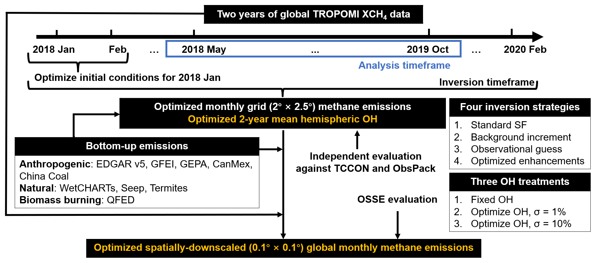
Figure 1 summarizes our inversion framework. We employ TROPOMI measurements from January 2018–February 2020 with the GEOS-Chem adjoint model in a suite of 4D-Var inversions to optimize monthly total methane emissions at 2∘ × 2.5∘ (latitude × longitude) resolution. These derived emissions are then spatially downscaled to 0.1∘ × 0.1∘. We omit the first and final 4 months from interpretation to further minimize initial condition errors and to ensure that all derived fluxes are adequately informed by subsequent observations. Our final analysis timeframe thus spans 18 months from May 2018 through to October 2019.
2.1 TROPOMI observations and independent evaluation datasets
TROPOMI was launched in October 2017 on board the Copernicus Sentinel-5 Precursor satellite into a low-Earth polar orbit and monitors greenhouse gases and air pollutants with daily near-global coverage at ∼ 13:30 LT (Equator overpass) on the ascending node (Hu et al., 2018). We use the SRON-corrected retrieval described in Lorente et al. (2021), which is based on the S5P-RemoTeC full-physics algorithm with albedo correction and updated regularization scheme, spectroscopic information, and surface treatment. This updated algorithm mitigates the albedo bias that affected earlier versions (Qu et al., 2021). Relative to the albedo-corrected product, the prior TROPOMI version exhibits high biases over North Africa, the Middle East, and the western US and low biases over Amazonia, the eastern US, central Africa, and eastern China (Lorente et al., 2021).
The TROPOMI total column (XCH4 in ppb) retrievals employ combined solar backscatter measurements in the near infrared (NIR; 0.8 µm) and shortwave infrared (SWIR; 2.3 µm) and have × 7 km2 nadir resolution on a 2600 km swath. The data have < 1 % nominal bias, 0.6 % instrument noise, and an estimated 0.8 % forward model error (Hu et al., 2016). We omit high-latitude (> 60∘) observations and require quality filter QA > 0.5 (Sentinel-5 Precursor/TROPOMI Level 2 Product User Manual: Methane, 2022) to avoid errors associated with high solar or viewing zenith angles, low surface albedo, excessive aerosol loading, clouds, terrain roughness, and measurement noise (Lorente et al., 2021). Figure 2 shows the resulting TROPOMI XCH4 data for March 2018–February 2020, gridded to 0.1∘ × 0.1∘ using the method described by Sun et al. (2018). In total, 91 million retrievals during May 2018–October 2019 pass quality filtering and are available for analysis, an average of 31 000 per 2∘ × 2.5∘ GEOS-Chem grid cell (Fig. S1). For inversions on the 2∘ × 2.5∘ model grid, we first average the TROPOMI observations to this resolution.
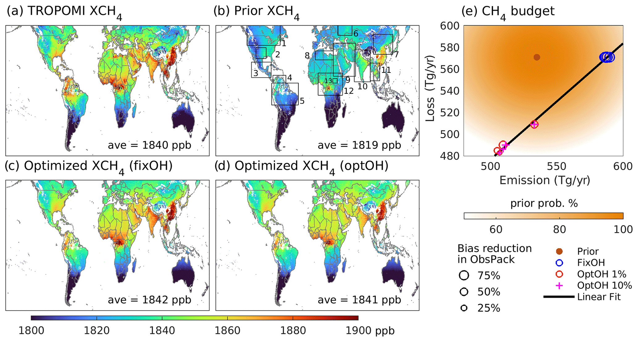
Figure 2Observed and simulated methane distributions for March 2018–February 2020. (a) TROPOMI methane column (XCH4) observations oversampled to 0.1∘ × 0.1∘. (b) Methane column distribution predicted by the prior model sampled according to the TROPOMI observation operator with numbered regions described in the text. (c) The same as panel (b) but for the fixOH optimized ensemble mean. (d) The same as panel (b) but for the optOH optimized ensemble mean. (e) Prior and optimized methane budgets. Prior probabilities (orange) equate 1 standard deviation to 25 % of the bottom-up range from Saunois et al. (2020), following Hozo et al. (2005). The black line shows a linear fit to the solution, emission = 0.93 × loss + 55.26 (units: Tg yr−1). Symbol sizes indicate the mean bias reduction against ObsPack independent measurements. Annual values are for November 2018–April 2019 plus the average of May–October 2018 and May–October 2019.
Figure S2 shows that TROPOMI measurements within our inversion timeframe agree well with independent measurements from the Total Carbon Column Observing Network (TCCON, 2014) and the Greenhouse Gases Observing Satellite (GOSAT, 2022), with major axis regression slopes of 1.02 (R=0.82) and 0.99 (R=0.88), respectively. The inter-dataset mean biases are −7.1 ppb (0.4 %, TROPOMI – GOSAT) and −5.4 ppb (0.3 %, TROPOMI – TCCON; see Text S1). Our initial condition optimization further ensures that the model and TROPOMI are unbiased with respect to each other so that mismatches arising during the simulation timeframe reflect source–sink disparities rather than any systematic observational bias.
We use a large suite of independent measurements to evaluate the inversions. These include methane columns from the TCCON (2014) network of Fourier transform spectrometers and methane mole fractions from the ObsPack (near-real time version v2.0; 2021) compilation of ground-based and airborne measurements. We further use CO and OH measurements from the Atmospheric Tomography (ATom) airborne campaign (Wofsy et al., 2018) to test inversion success at separately optimizing methane sources and sinks. ATom featured pole-to-pole profiling (0.2 to 12 km) during four seasons over 4 years. The flight design is thus well suited to determine whether the optimized OH fields improve or degrade global model simulations of OH itself and of CO (whose dominant sink is reaction with OH). Measurements of CO during ATom were performed using the NOAA Picarro instrument with an estimated uncertainty of 3.6 ppb (Chen et al., 2013). OH measurements during ATom employed the Airborne Tropospheric Hydrogen Oxides Sensor (ATHOS), with an estimated uncertainty of 0.018 ppt (1 min average; Brune et al., 2020).
2.2 Forward model and initial conditions
We use the GEOS-Chem adjoint model (v35), on a 2∘ × 2.5∘ grid with 47 vertical layers, to perform the global 4D-Var inversions. The model uses GEOS-FP meteorological fields from the National Aeronautics and Space Administration (NASA) Global Modeling and Assimilation Office (GMAO, 2013), with 5 and 10 min time steps for transport and emissions, respectively. Transport employs fully instantaneous boundary layer mixing (Wu et al., 2007), a relaxed Arakawa–Schubert convection scheme (Moorthi and Suarez, 1992), and a multi-dimensional flux-form semi-Lagrangian (FFSL) treatment for advection (Lin and Rood, 1996). For all model-satellite comparisons (and at each inversion iteration) the GEOS-Chem output is sampled according to the TROPOMI observation operator at the overpass time and location.
We optimize the model initial conditions for 1 January 2018 in three steps, first starting with a 25-year global spin-up to achieve a globally representative methane field. We then apply a latitude-dependent correction based on the TROPOMI–model difference for November 2017–January 2018 to speed up the optimization process in the next step. Correction over land employs the median TROPOMI–model difference by latitude; over oceans (which lack TROPOMI XCH4 data) we use the 0.1 quantile difference. Finally, we optimize the resulting fields in a 4D-Var inversion based on TROPOMI data for January–February 2018. The optimized global methane burden is 0.99× that in the original 25-year spin-up, and the north : south hemispheric (NH : SH) XCH4 ratio increases from 1.11 to 1.13.
2.3 Prior model sources and sinks
Global anthropogenic methane emissions in the prior model use the gridded United Nations Framework Convention on Climate Change (UNFCCC) inventory for fossil fuels (year 2016; GFEI, Scarpelli et al., 2020) and Emissions Database for Global Atmospheric Research (EDGAR) v5 for other sources (year 2015; Crippa et al., 2019, 2020). These are superseded by the 2012 GEPA inventory for US anthropogenic emissions (Maasakkers et al., 2016), the CanMex inventory for Canadian (year 2013) and Mexican (year 2010) oil and gas emissions (Sheng et al., 2017), and for Chinese coal mine emissions (year 2011) (Sheng et al., 2019). Wetland emissions use the 2018–2019 WetCHARTs ensemble mean flux (Text S2; Bloom et al., 2017), scaling the total to 149 Tg yr−1 to match the 2008–2017 global methane budget from Saunois et al. (2020). We apply Fung et al. (1991) and Maasakkers et al. (2019) for termite and geological seep emissions, respectively, and employ biomass burning emissions for 2018–2019 from the Quick Fire Emissions Dataset (QFED, Darmenov and Silva, 2015; Koster et al., 2015). Figure S3 maps these prior emissions, which total 535 Tg yr−1 and include 356 Tg yr−1 from anthropogenic sources (119 Tg yr−1 livestock, + 101 Tg yr−1 fossil fuel, + 80 Tg yr−1 waste, + 37 Tg yr−1 rice, + 19 Tg yr−1 other), 165 Tg yr−1 from natural sources (149 Tg yr−1 wetlands, + 16 Tg yr−1 geological seeps and termites), and 14 Tg yr−1 from biomass burning. Emissions from EDGAR v5 vary monthly based on national and sub-national sectoral activity levels. GEPA includes monthly emission profiles for US rice and manure management, and we assume aseasonal emissions for indoor animal husbandry following Crippa et al. (2020). The WetCHARTs emissions are monthly, reflecting temporal changes in wetland extent, respiration, and temperature. QFED emissions are daily with an hourly diel profile applied.
Atmospheric methane removal by OH (87 % of the total sink, 494 Tg yr−1) in the prior model uses archived monthly oxidant fields from GEOS-Chem (v5) benchmark simulations (Wecht et al., 2014), which have an annual tropospheric air-mass-weighted mean of 1.03 × 10⁶ molec. cm−3 and a 1.04 NH : SH ratio. Other minor sinks include stratospheric oxidation (6 %, 33 Tg yr−1) based on NASA's Global Modeling Initiative monthly loss frequencies (Murray et al., 2013), soil uptake (6 %, 34 Tg yr−1) following Fung et al. (1991), and tropospheric oxidation by chlorine (2 %, 10 Tg yr−1) using 3D monthly Cl fields from Sherwen et al. (2016). The above sinks total 571 Tg yr−1 (Fig. 2e) and yield a 9.1-year methane lifetime in our prior simulations.
Simulations to evaluate posterior model performance for CO and OH employ anthropogenic emissions (for CO, NOx, and VOCs) from the Community Emissions Data System (Hoesly et al., 2018), the 2016 EPA National Emissions Inventory (NEI) v1 (NEIC, 2019), and the Air Pollutant Emission Inventory (APEI, 2020). Corresponding biogenic and biomass burning emissions are obtained from the Model of Emissions of Gases and Aerosols from Nature (MEGANv2.1; Hu et al., 2015), and QFED (Koster et al., 2015).
2.4 Inversion frameworks and sensitivity to OH
Optimizations are performed in the GEOS-Chem adjoint model (Henze et al., 2007) through iterative minimization of the Bayesian cost function J(x):
The first right-hand term imposes a penalty based on the deviation of x (the state vector to be optimized) from xa (the prior estimates), weighted by the prior error matrix Sa. The state vector x includes monthly 2∘ × 2.5∘ grid-level emissions and (in some cases) the 2-year-mean hemispheric loss to OH. This penalty is counteracted by the second right-hand term, which reflects the mismatch between the observations y and model predictions F(x) sampled in the same manner, weighted by the observing system error matrix So. The regulation parameter γ is applied to balance the influence of the above two terms in the overall cost function J(x). Our inversions run continuously from January 2018 to February 2020, optimizing monthly grid-total methane emissions and 26-month mean hemispheric OH concentrations. To minimize any effects from initial conditions and to allow for sufficient observational constraints throughout the analysis period, we focus interpretation on the 18-month period from May 2018 to October 2019. Annual values discussed later are for November 2018–April 2019 plus the mean of May–October 2018 and May–October 2019.
The prior error covariance matrix Sa for methane emissions is constructed as follows. We use Maasakkers et al.'s (2016) scale-dependent uncertainties for anthropogenic emissions over the GEPA and CanMex domain, as well as Sheng et al.'s (2019) province-level error estimates for Chinese coal mine emissions. For other global anthropogenic emissions we use the gridded fossil fuel uncertainty estimates from Scarpelli et al. (2020) and assume 50 % uncertainty in the remaining sources (Maasakkers et al., 2019; Yu et al., 2021c). Uncertainties for wetland emissions are derived as 1 standard deviation across the WetCHARTs ensemble, averaging 105 % at the grid level. Other sources employ a prior error standard deviation of 50 %, consistent with earlier studies (Maasakkers et al., 2019; Sheng et al., 2018; Turner et al., 2015; Wecht et al., 2014; Yu et al., 2021c). The diagonal of the prior error matrix combines the above flux-weighted terms in quadrature and averages 66 %. We find that the spatial covariance in the total prior emissions decreases by 50 % over a mean distance of approximately 300 km, and we populate the exponentially decaying off-diagonal elements of Sa accordingly. This is comparable to the 200–500 km correlation length scales applied in previous methane studies (Monteil et al., 2013; Wecht et al., 2014; Yu et al., 2021c).
We test the impacts of OH on our results through three separate inversion treatments: the first uses the prior OH with no optimization, while the second and third optimize methane loss to OH on a hemispheric basis with an assigned uncertainty (included in Sa) of either 1 % or 10 % (Prather et al., 2012; Saunois et al., 2020). We find that both the 1 % and 10 % uncertainty assumptions for OH give effectively identical inversion solutions: in both cases the optimization has sufficient OH flexibility to correct a global mean budget imbalance on that basis, with the remaining spatial errors resolved through grid-level emission adjustments (Fig. S4). We therefore mainly discuss results from the 1 % optimization (referred to as optOH), along with those from the fixed OH (fixOH) inversion. Other minor sinks, such as soil uptake, are also uncertain but not addressed here.
Observing system errors combine measurement errors and forward model errors. Building on Heald et al. (2004), we compute the elements of So (which is diagonal) from the residual standard deviation between the observations and the prior simulations within a 2∘ × 2∘ moving window, further imposing a lower bound of 56 ppb2 (0.25 quantile of the overall results). The resulting observing system errors average 11 ppb, mainly reflecting instrument noise, and are comparable to previous estimates for GOSAT and TROPOMI (11–13 ppb; Maasakkers et al., 2019; Zhang et al., 2020).
The regulation parameter γ is defined through sensitivity inversions for January 2018 with γ varying from 10−5 to 103. The optimal monthly value is selected based on the resulting L curve and total error reductions (Fig. S5) and then scaled to the number of observations for the full 2-year inversion period. The result (γ=0.03) is consistent with previous TROPOMI inversions by Qu et al. (2021) (γ=0.002) given their optimization of annual rather than monthly emissions.
Adjoint 4D-Var inversions do not directly provide posterior error estimates. Methods are available to indirectly derive such estimates (Bousserez et al., 2015; Yu et al., 2021a); however, our previous observing system simulation experiments (OSSEs; Yu et al., 2021a) showed that for methane the computed posterior error reductions do not correlate with more accurate flux estimates in the presence of model transport errors and spatially inaccurate prior emissions. Here, we instead combine multiple inversion strategies (Sect. 2.5) with an ensemble of independent observations (Sects. 2.1, 3) to test the robustness of our results and characterize the associated uncertainties.
Recent inverse analyses by Qu et al. (2021) likewise examined the global methane budget using TROPOMI (and GOSAT) observations. Our study advances on that work in several ways. First, we optimize monthly rather than annual fluxes to identify seasonal patterns of variability. Second, in place of a traditional analytical optimization we combine 4D-Var with new inverse formalisms for better identification of missing sources. Third, we develop a new downscaling approach to constrain emissions at high resolution and use this framework to elucidate flux mechanisms and missing sources. Finally, our analysis leverages an updated TROPOMI methane product (Lorente et al., 2021) that corrects an albedo-dependent bias present in the version used by Qu et al. (2021).
2.5 Inversion ensemble to explore sensitivity to missing sources
Our previous OSSE-based work (Yu et al., 2021a) emphasized that classical scaling factor (SF)-based inversions have limited ability to recover missing sources. Here, we apply multiple inversion formalisms to diagnose and address this issue:
-
Classical SF inversions (SF). SF inversions employ the bottom-up inventories described earlier as prior. These inversions solve for scale factors s in .
-
Background increment inversions (BI). BI inversions employ a revised prior consisting of the above inventories scaled by 90 % plus the remaining 10 % as a uniform overland flux. This revised prior is then subjected to SF optimization.
-
Observational guess inversions (OG). OG inversions employ a revised prior informed by long-term TROPOMI data for better recovery of missing sources. Specifically, we find from sensitivity simulations that adding 75 Tg yr−1 to the bottom-up emissions results in a globally unbiased simulation across 2018–2020. We distribute this 75 Tg yr−1 spatially based on the observation-model enhancement mismatches, where the grid-level enhancements are computed as the local XCH4 value minus the zonal mean (2∘ bins). Figure S6 shows the resulting grid-level emission increments.
-
Emission enhancement inversions (EE). EE inversions solve for absolute flux increments rather than scale factors via . We define xbase as 2600 kg per box per time step, which is the mean emission for grid cells exceeding 1 kg per box per time step. We showed previously that this approach has better performance for missing sources than the above three SF inversions (Yu et al., 2021a).
In the following, we interpret the multi-inversion mean as our base-case solution and the range as the corresponding uncertainty estimate.
2.6 Emission downscaling
We present here a new method to spatially downscale the satellite-derived emissions from 2∘ × 2.5∘ to 0.1∘ × 0.1∘ for potential use in models. The downscaling, which combines information from the TROPOMI column enhancements, the prior emission estimates, and their uncertainties, is necessitated by the fact that the current GEOS-Chem adjoint model does not have global simulation capability at finer than 2∘ × 2.5∘ resolution. Furthermore, each of the 2-year inversions performed here required > 12 000 CPU hours (> 80 d on multiple processors) to converge, making higher-resolution optimizations computationally impractical. However, the inventories employed as prior, as well as the TROPOMI observations themselves, contain information at much finer scales (e.g., 0.1∘ × 0.1∘ and 7 × 7 km2) – and thus contain additional high-resolution constraints that are neglected by the 2∘ × 2.5∘ inversions. We therefore leverage this information to spatially downscale the optimized emissions to 0.1∘ × 0.1∘ via
Equation (2) downscales the original optimized emissions from a given 2∘ × 2.5∘ parent grid cell i to the subgrid scale (xj′ at 0.1∘ × 0.1∘) by combining spatial information from the observations (first right-hand term) and the prior (second right-hand term). Here, ωi is a weighting factor to balance these two terms; and are spatial downscaling operators representing the observational and prior information, respectively; represents the 0.1∘ × 0.1∘ prior emissions for subgrid j; and si is the 2∘ × 2.5∘ scale factor derived for parent grid cell i.
The observational downscaling operator spatially allocates the subgrid-level emissions according to the distribution of column enhancements over the regional background:
where y2y,j is the 2-year mean (March 2018–February 2020) TROPOMI methane column sampled to 0.1∘ × 0.1∘ (Sun et al., 2018), and ybg,i is the methane background defined as 95 % of the y2y,j 0.1 quantile across the parent 2∘ × 2.5∘ grid cell i. This background definition was determined via OSSE analysis (described below), with the corresponding parameters varied systematically over a wide range to identify values yielding the best consistency with the true underlying fine-scale emissions. fk quantifies the prior fraction of total 2∘ × 2.5∘ emissions contained in each subgrid k∈j.
The prior downscaling operator spatially allocates the derived flux enhancement si−1 based on the prior emission magnitudes and their uncertainties:
where is the prior emission error estimate at 0.1∘ × 0.1∘. In this way larger corrections are preferentially assigned to locations with higher prior emissions and uncertainties.
When summed to 2∘ × 2.5∘, both the prior and observational downscaling terms maintain the original adjoint-derived emissions. Weighting between these terms is computed as
where εa,i is the prior emission error estimate at 2∘ × 2.5∘, and is the log-transformed standard deviation of all 0.1∘ × 0.1∘ prior emissions contained in that parent grid cell (with an imposed zero lower bound). As shown in Fig. S7, the resulting downscaling relies most frequently on the prior information, particularly for low-emission areas, but hotspots and locations with higher prior uncertainties are preferentially informed by the observations.
Compared to existing emission downscaling methods that rely on prior and posterior error covariance estimates (Cusworth et al., 2021), or are based solely on satellite data (Liu et al., 2021), our approach is unique in combining the prior emission information (and its uncertainty) with the oversampled TROPOMI observations themselves. Variable weighting between these terms permits greater influence from the observations when the prior emissions are more uncertain. The method thus assumes robust prior error estimates, a caveat that also applies to Cusworth et al. (2021) and similar methods.
We tested the effectiveness of this downscaling approach in a 1-month OSSE analysis over North America (which features all relevant source types and a computationally tractable model domain). These synthetic inversions follow Yu et al. (2021a) in prescribing true and prior emissions from distinct inventories (true: gridded EPA + WetCHARTs ensemble mean; prior: EDGAR v5 + a single WetCHARTs member) that differ by 76 Gg d−1 domain-wide and have spatial R=0.51 at 0.25∘ × 0.3125∘. The OSSEs were performed at 2∘ × 2.5∘ by sampling the true-state model according to the TROPOMI coverage for August 2018 (with measurement noise applied), followed by 4D-Var optimization as detailed by Yu et al. (2021a). The 2∘ × 2.5∘ adjoint solution was then spatially downscaled to 0.25∘ × 0.3125∘ following Eq. (2) and compared to both the true fluxes and to the adjoint solution performed directly on the fine-scale grid. Tests were performed both in the presence and absence of model transport error (Yu et al., 2021a).
Table 1 shows that in the absence of transport error our downscaling approach outperforms the coarse-grid solution and approaches the skill of the native fine-scale inversion in representing the true fluxes. The benefits of the 4D-Var + downscaling approach are even more pronounced when accounting for transport error. Specifically, our previous OSSE analyses showed that high-resolution 4D-Var inversions failed to improve methane emission estimates at 25 km for scenarios with both transport error and spatially biased emissions (Yu et al., 2021a). Our tests here show that spatial downscaling of the 2∘ × 2.5∘ adjoint solution strongly mitigates these effects (Table 1), yielding a larger bias reduction (98 % versus just 16 %) and more accurate flux distribution (R=0.70 versus 0.60) than the native fine-grid 4D-Var solution. Figure S8 further shows that the downscaled OSSE solution reduces the prior bias by 17 %–56 % for sources exceeding 1000 kg CH4 per box per day (accounting for 99 % of the domain-wide emissions) when not subject to transport error. In the presence of transport error, the downscaling method has limited improvement for the very largest sources (> 2× 10⁵ kg per box per day) but nevertheless exhibits strong bias reduction (21 %–50 %) for sources between 1 × 10³–2× 10⁵ kg per box per day (which account for 96 % of domain-wide emissions). Given these results and the finer-scale information available here, for the present work we apply Eq. (2) to spatially downscale our inversion solutions to 0.1∘ × 0.1∘.
Table 1Downscaling performance evaluation via OSSE1.
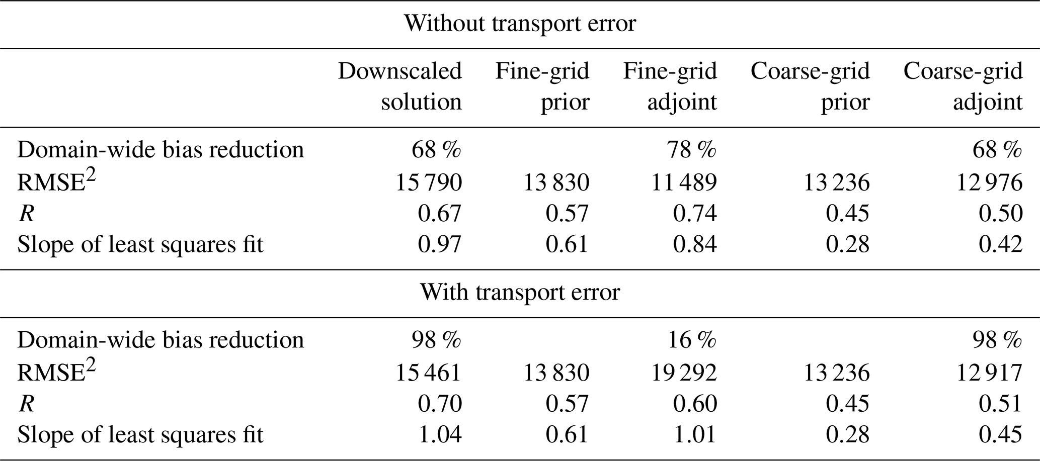
1 Observing system simulation experiments performed for 1 month over North America. 2 Root mean square error, units: kg per day per box.
3.1 Methane source–sink ambiguity
The set of inversion configurations includes multiple formalisms for emission adjustment and two separate treatments for methane loss: fixOH inversions use the prior OH as a fixed constraint, while optOH inversions optimize both OH concentrations (as a 2-year hemispheric mean) and methane emissions. Figure 2 shows that the fixOH and optOH multi-model means yield similar atmospheric methane distributions, with the strongest enhancements over central Africa, South and East Asia, the Middle East, Amazonia, and the southern US and the lowest column concentrations over high southern latitudes in Australia, South America, and Africa. The two approaches also provide comparable improvement with respect to the TROPOMI observations, with > 97 % mean bias reduction and > 45 % root mean square error (RMSE) reduction.
Despite the above patterns of agreement, the fixOH and optOH inversions lead to opposing methane emission changes relative to the prior budget. The fixOH multi-model mean provides a global methane source of 587 Tg yr−1 (10 % higher than the prior) and a sink of 571 Tg yr−1. The optOH multi-model mean yields a 514 Tg yr−1 source (4 % below the prior) and a 492 Tg yr−1 sink; the latter is driven by updated OH fields with an air-mass-weighted NH:SH ratio of 0.98. Figure 2e shows that the fixOH and optOH solution sets adhere closely to a linear relationship between global sources and sinks, in all cases with a ∼ 20 Tg yr−1 growth rate in the atmospheric methane burden.
While mutually inconsistent, the fixOH and optOH global methane sink terms are each physically tenable, falling, respectively, towards the high- and low-end estimates of Saunois et al. (2020) top-down budget assessment for 2008–2017 (501–574 Tg yr−1). The OH fields dominating methane removal in these two scenarios are likewise physically viable based on available independent constraints. If we attribute the optOH methane loss correction entirely to OH, we arrive at global mean [OH] = 8.27 × 10⁵ molec. cm−3, placing the fixOH (1.03 × 10⁶ molec. cm−3) and optOH solutions near the middle and lower end of the range indicated by prior assessments (0.85–1.30 × 10⁶ molec. cm−3; Krol and Lelieveld, 2003; Li et al., 2018; Montzka et al., 2011; Naik et al., 2013; Patra et al., 2021; Prinn et al., 2001, 2005; Rigby et al., 2017; Zhao et al., 2019). Our 2018–2019 analysis timeframe also spans an El Niño, which has been tied both to global OH decreases and to methane growth rate acceleration (Anderson et al., 2021; Turner et al., 2018a) – further complicating a differentiation between the fixOH and optOH solutions.
Additional ambiguity arises from the fact that the optOH methane sink adjustments could partly reflect uncertainty in the CH4+ OH rate coefficient, which here follows Burkholder et al. (2020). While the rate at 298 K has been verified to within 1 % across many lab experiments, uncertainties increase for higher and lower temperatures (up to 13 % within 273–313 K, Burkholder et al., 2020). Given all of the above considerations, we turn to independent measurements of methane, CO, and OH to assess the fixOH versus optOH solution fidelity.
3.2 Independent model assessments to discriminate between conflicting methane budgets
Ground-based methane column (XCH4) observations from the TCCON network (GGG2014; 2014) show comparable improvements over the prior for both the fixOH and optOH solutions (and for their individual member inversions), with 71 % (from −12.9 ppb to 3.8 ppb) and 66 % (to 4.3 ppb) mean bias reductions, respectively (Fig. 3, Table S1). However, global in situ measurements from ObsPack (near-real time version v2.0; 2021) reveal a 93 % (from −13.8 to −0.9 ppb) absolute mean bias improvement for the fixOH framework compared to just 39 % (to 8.4 ppb) for optOH (Fig. 3, Table S1). Figure 3 further shows that the optOH solutions overcorrect the prior negative bias with respect to ObsPack, providing a first piece of evidence for a methane sink underestimate in this inversion.
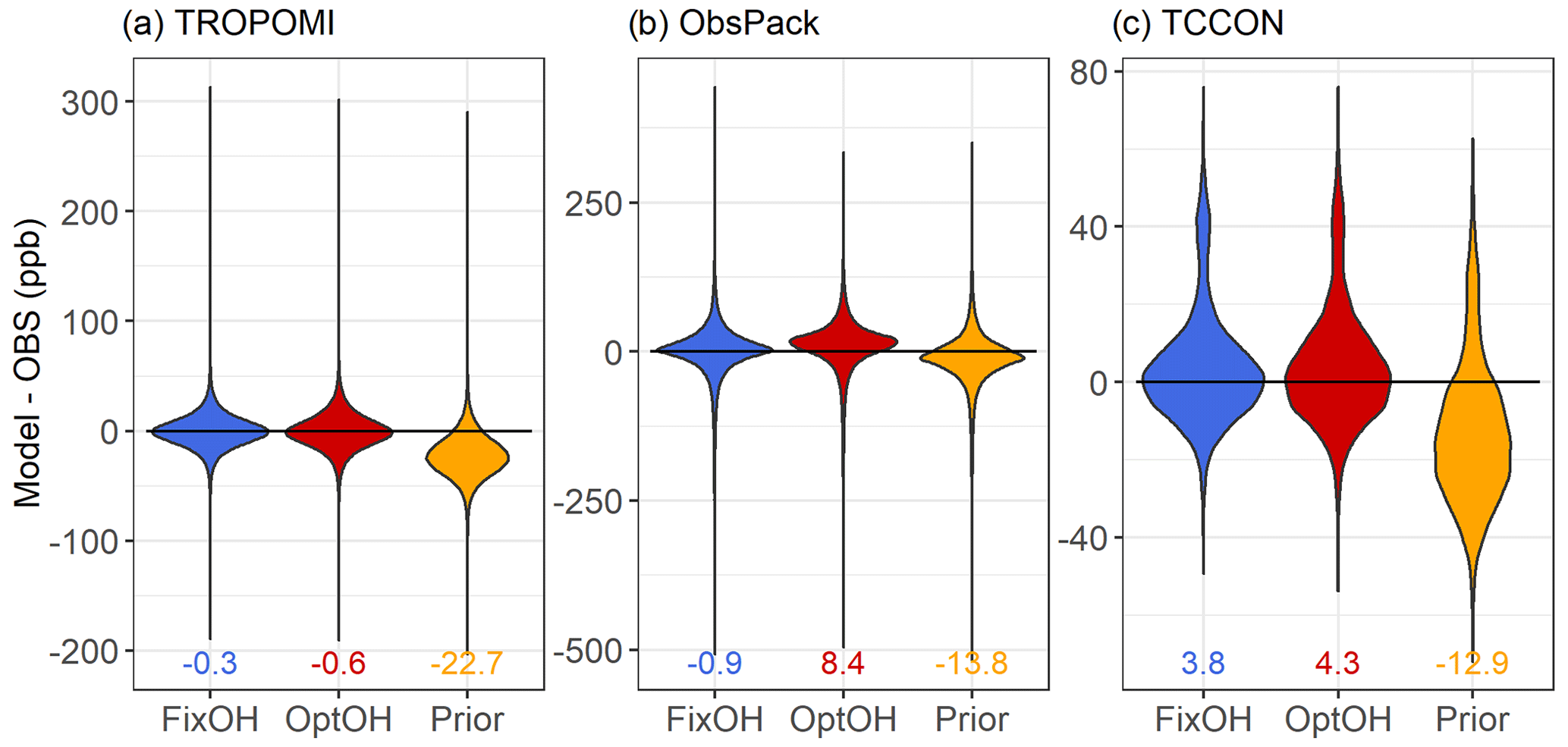
Figure 3Evaluation of the prior and optimized methane simulations (May 2018–October 2019) against (a) TROPOMI XCH4 observations, (b) ObsPack in situ methane measurements, and (c) TCCON ground-based methane column observations. Numbers inset indicate the mean model-observation bias (unit: ppb).
Remote observations of OH and CO (the primary OH sink) from the ATom airborne campaign (Wofsy et al., 2018) also point to an OH underestimate in the optOH solution. Figure S9 compares the ATom observations for these species with predictions from supplemental GEOS-Chem simulations (configured as in Gonzalez et al., 2021) constrained to the fixOH and optOH oxidant fields. With the exception of ATom 3, the mean model OH biases with respect to ATom observations are ∼ 80 % lower for fixOH than for optOH (mean differences are all significant based on a paired t test at 95 % confidence). These optOH results exhibit a consistent OH underestimate (averaging 0.020–0.044 ppt) that exceeds the 0.018 ppt measurement uncertainty. Biases in the simulated background CO levels are likewise lower (by 7 %–87 %) in the fixOH simulations, with a clear CO overestimate for optOH (Fig. S9). Again, the mean fixOH optOH differences are all statistically significant at the 95 % confidence level, with model-measurement discrepancies for optOH (7–12 ppb) exceeding the 3.6 ppb measurement uncertainty. While the ATom timeframe (2016–2018) is distinct from that of the TROPOMI inversions (2018–2019), the model is sampled at the time of measurement for both comparisons. We therefore expect the OH and CO biases highlighted above to likewise manifest for 2018–2019 – an expectation that is supported by the ObsPack comparison.
When co-optimizing methane emissions and loss we thus find that the solutions can achieve a good fit to the TROPOMI data themselves but degrade model agreement with other observations of methane, OH and CO. We conclude that solving for global methane sources and sinks based solely on satellite observations of methane itself remains an unconstrained problem – even with the dense TROPOMI data coverage. In the same way, previous studies using methane data to optimize OH alongside emissions are likely subject to strong error correlations between the derived sources and sinks (Lu et al., 2021; Maasakkers et al., 2019; Qu et al., 2021; Zhang et al., 2018, 2021). On the other hand, the comparisons here provide robust support for the fixOH inversion solutions based on their fidelity against independent atmospheric observations.
We thus focus the remainder of this paper on the fixOH results and treat the corresponding multi-model mean as our base-case solution. The fixOH constituent inversions (scale factor – SF, background increment – BI, observational guess – OG, and emission enhancement – EE) each employ an alternative framework for spatial emission correction, as described earlier. Figure S10 shows that these individual members converge closely (within 0.5 %) in terms of the total derived methane flux, with a high degree of spatial similarity in their derived emissions. Differences in adjustment magnitudes emerge, with the OG and EE frameworks generally yielding the largest and smallest emission corrections, respectively. Overall, the derived grid-level emissions agree to within 30 % for 42 % of the emitting model grid cells, with consistent adjustment direction over areas encompassing 65 % of the total optimized emissions. In what follows we focus discussion on these areas of consistency and use the multi-model spread to draw insights into some of the key disparities.
We infer from the TROPOMI observations an optimized global methane flux of 587 (586–589) Tg yr−1 for 2018–2019, including 375 (367–387) Tg yr−1 from anthropogenic sources, 197 (185–207) Tg yr−1 from natural sources, and 15 (14–15) Tg yr−1 from biomass burning. Values listed reflect the fixOH multi-model mean and range, with emissions partitioned to individual sources according to the prior grid-level sectoral fractions. Our derived natural source falls at the low end of the 2017 Global Methane Project estimates (GMP; 194–489 Tg yr−1), whereas we infer a larger source from agriculture and waste than GMP does (253–262 versus 198–246 Tg yr−1) (Jackson et al., 2020). The TROPOMI-derived methane emissions from fossil fuel and industry of 118 (112–127) Tg yr−1 lie between the GMP top-down (91–121 Tg yr−1) and bottom-up (121–164 Tg yr−1) estimates for that sector. Jackson et al. (2020) attributed the global methane emission increase between 2000–2006 and 2017 mainly to anthropogenic sources, with similar contributions from agriculture/waste and fossil fuel. Here, we find that emissions from agriculture and waste are even larger than estimated by GMP.
Table 2 lists the top 10 national contributors to global anthropogenic methane emissions (see Table S2 for natural and total emissions). Together, we find that these contributors account for 58 % of the global anthropogenic flux, and they similarly represent 60 % of the global population. However, within this group there are large differences in per capita emissions, which are 72 %–286 % higher than the global average in Brazil, the US, Russia, and Iran but 17 % lower in China and 45 % lower in India. Table 2 also includes three of the five countries with the largest natural methane emissions, largely from wetlands: Brazil (39 Tg yr−1), the US (16 Tg yr−1), and Russia (12 Tg yr−1). Together with the Republic of the Congo (22 Tg yr−1) and Canada (15 Tg yr−1) these countries account for 53 % of natural methane sources globally. This places Brazil (59 Tg yr−1) and the US (43 Tg yr−1) as the second- and third-largest methane emitters in terms of total flux, after China (61 Tg yr−1, 94 % anthropogenic; Table S2).
Table 2Top 10 contributors to global anthropogenic methane emissions.1,2
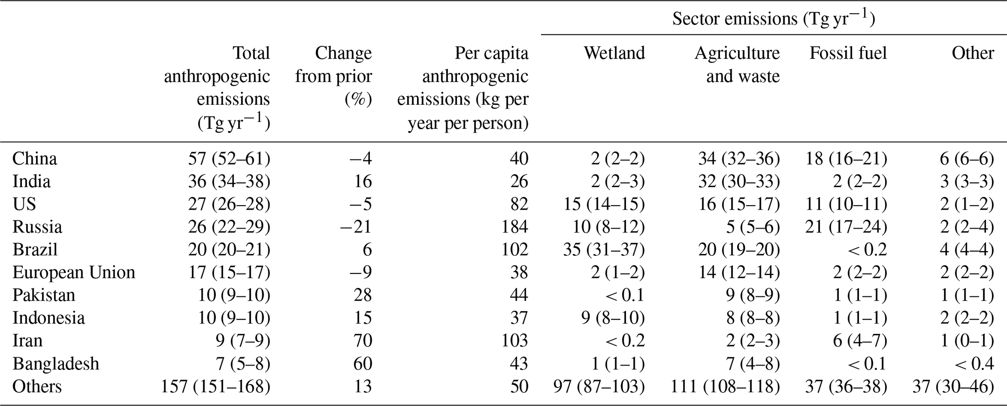
1 This is based on the fixOH inversion ensemble mean and range. 2 Values in parentheses indicate the range in emission estimates across the suite of inversions.
In total 8 of the 10 nations in Table 2 (China, India, the US, Russia, Brazil, the European Union, Pakistan, Indonesia) are likewise identified by Worden et al. (2022) as among the top 10 anthropogenic emitters globally. Our inferred anthropogenic fluxes for the US and China agree well (within ∼ 10 %) with the GOSAT-based results from Worden et al. (2022) and with the GOSAT + TROPOMI results from Qu et al. (2021). Anthropogenic emissions derived here are likewise within 10 % of Worden et al.'s (2022) results for India and the European Union, with both studies lower (20 %–50 %) than Qu et al. (2021). Our results for Russia and Iran are 21 %–28 % higher than the GOSAT-based estimates, mainly reflecting oil, gas, and coal emissions and ∼ 40 % lower for Brazil, mainly due to livestock. Emissions for Pakistan and Indonesia agree to within 1 % for the TROPOMI- and GOSAT-based results (Worden et al., 2022). However, we find here that anthropogenic emissions from Bangladesh (7 Tg yr−1 versus a prior of 4 Tg yr−1) are 3× higher than the GOSAT estimate (2 Tg yr−1), while adjacent emissions from Myanmar (4 Tg yr−1) are half the GOSAT estimate. Worden et al. (2022) conclude that the GOSAT-derived emissions for Myanmar are anonymously high due to impacts from their prior assumptions; we attribute much of that flux to Bangladesh and show later that it mainly arises during the South Asian monsoon.
The TROPOMI-derived wetland fluxes (excluding rice) total 173 (155–182) Tg yr−1 globally, representing 29 %(26 %–31 %) of the total methane source and 88 % (84 %–91 %) of the natural source. Figures S3, S11, and 4e show that global wetland emissions are lowest during October–February (12–13 Tg per month) and highest in July (17 Tg per month) due to strong Northern Hemisphere seasonality. We find through the inversions that global wetland fluxes are 24 Tg yr−1 higher than the prior estimate, with the increase mainly originating in the tropics (82 % within ± 23.5∘ latitude). The tropics thus account for 70 % (68 %–72 %) of our optimized wetland emissions. Northern temperate wetlands contribute most of the remainder (46 Tg yr−1 from 23.5–66.5∘ N) with a magnitude that is in line with the prior bottom-up estimate (44 Tg yr−1). Our derived global wetland fluxes are ∼ 20 % higher than previous GOSAT-based estimates (145–148 Tg yr−1: Ma et al., 2021; Zhang et al., 2021), with similar latitudinal distribution to that found by Ma et al. (2021).
Over Amazonia (box 5 in Fig. 2b), we obtain wetland fluxes of 51 (44–54) Tg yr−1, 29 % of the global wetland total. These fluxes are underestimated in the WetCHARTs prior inventory by 9 (2–11) Tg yr−1; the true disparity is likely even larger, since the inversions do not fully mitigate the prior regional XCH4 bias (Fig. 2c). Low observation density due to clouds (Fig. S1) leads to some ambiguity in the spatial distribution of these derived fluxes: the SF and BI inversions allocate the upward corrections according to the prior spatial patterns over Amazonia, while the OG inversion identifies broader sources extending to northern Brazil (Figs. 4 and S10). Upward corrections occur mainly during the wet season (December–April) and are temporally correlated with runoff (mean monthly R=0.85, ERA5, 2019). This strong dependence on hydrology is likewise seen in the GOSAT-inferred flux increases over Amazonia that has been linked to increased flooding with strengthening Walker circulation (Barichivich et al., 2018; Zhang et al., 2021). However, eastern Brazil is also an agricultural frontier with forests transitioning to agricultural lands (Nepstad et al., 2019; Zhang et al., 2021), and our inversions point to a 9 % (5 %–15 %) underestimate of Amazonian livestock sources. Bottom-up calculations suggest a 33 % increase in this source from 2010–2018 (EDGAR v6, 2021); if such trends are in fact underestimated then our prior-based partitioning would imply an even larger livestock contribution to the derived regional emission corrections.
The inversions also point to a substantial (26 % [5 %–36 %]) upward correction for central African wetlands (box 12 in Fig. 2b) that is concentrated during December–May (Fig. S12). The optimized regional emissions are then 33 (28–36) Tg yr−1, 19 % of the global wetland total. However, while these adjustments effectively correct the prior model bias for this latitude band, there is a clear XCH4 overcorrection for the Democratic Republic of the Congo (DRC; Fig. 2c). Here, the modeled XCH4 enhancement over the background (Fig. S13) is degraded from a prior model-observation mismatch of +3 to +11 ppb. The low data density over central Africa and Amazonia (Fig. S1) thus appears to cause some tropical flux misattribution – with the DRC overcorrection offset by under-corrections over Amazonia (as discussed above), Nigeria, and the nearby Sudd wetlands (Fig. 2c). The latter region is examined further below.
Figure 2a shows that the south Sudd wetlands (box 13 in Fig. 2b) are a major methane hotspot that is underestimated in the prior model by a column average of 41 (21–65) ppb. Despite this, we derive a regional upward emission correction of just 13 % (optimized flux: 1.3 [1.2–1.4] Tg yr−1). This yields a residual underestimate (Fig. 2c), reflecting the aliasing discussed above and showing that the optimized south Sudd fluxes are still too low. Anomalous hydrology may contribute to these elevated Sudd fluxes: wetland extent for this area was ∼ 10 % higher in 2019 than the 2010–2019 mean (Jensen and Mcdonald, 2019), and ERA5 reanalysis (2019) points to elevated precipitation over central Africa during September–November (22 % above the 2010–2019 mean). This interpretation is consistent with a previous study by Lunt et al. (2021) linking anomalous East Africa rainfall during the 2018 long rains (March–May) and 2019 short rains (October–December) with 10 %–40 % methane emission increases over the south Sudd. Over longer timescales, GOSAT analysis has pointed to a 3 Tg yr−1 emission increase over the broader Sudd region caused by increased inflow from the White Nile and Sobat rivers (Lunt et al., 2019; Maasakkers et al., 2019; Parker et al., 2020). Previous SCIAMACHY- and TROPOMI-based analyses have likewise identified concentration hotspots over this area (Hu et al., 2018; Frankenberg et al., 2011).
North American wetlands in Alberta, Saskatchewan, and the US Upper Midwest are revised downward (by −1.6 [−0.7 to −2.6] Tg yr−1 for box 1 in Fig. 2b), with most of the adjustment occurring during early summer (−18 % for June–July vs. −1 % for August–September; Fig. 4). We thus obtain optimized regional wetland emissions of 16 [15–17] Tg yr−1, 9 % of the global flux from this source. Wetland emissions over this area are highly sensitive to soil temperature and surface water extent (R> 0.7 and R> 0.4, respectively; Fig. 5). The stronger June–July adjustment derived here suggests that the post-thaw onset of northern wetland fluxes occurs too early in WetCHARTs, which uses surface skin rather than soil temperatures to predict emissions. Similar downward emission corrections have been inferred from GOSAT (Zhang et al., 2021), aircraft, and long-term eddy covariance measurements (Yu et al., 2021c).
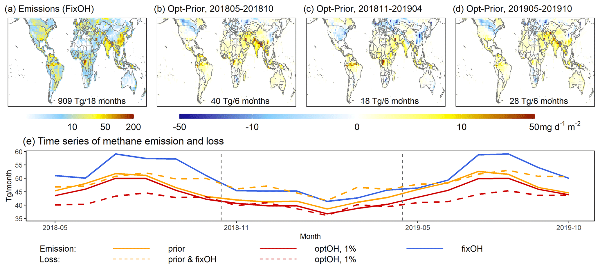
Figure 4(a) Optimized global methane emissions based on the fixOH inversion ensemble. (b–d) Seasonal fixOH emission corrections. Dots indicate missing sources where the EE and BI inversions point to positive corrections that the SF inversion misses. (e) Time series of prior and optimized methane sources and sinks.
Across the wetland regions examined above, Fig. S14 shows that our optimized emissions fall towards the middle of the land-surface model estimates from the Global Carbon Project (GCP; details on these bottom-up models and their differences are provided by Saunois et al., 2020). Among the GCP bottom-up estimates, we see in Fig. S14 that simple model parameterizations can obtain comparable agreement with the TROPOMI-optimized emissions as more complete process-based models. For example, LPJ-WSL, a parsimonious model that predicts net emissions based on soil characteristics without explicitly representing oxidation, transport, or wetland plant types, achieves similar fidelity (in terms of bias and RMSE versus the optimized values) as JSBACH (Kleinen et al., 2020), which features more sophisticated treatment of soil carbon, roots, and plant-mediated processes. Many simple wetland models rely on reanalysis-based wetland extent estimates such as the Global Lakes and Wetlands Database (GLWD) (Lehner and Döll, 2004); within the WetCHARTs ensemble we find here that GLWD-based flux predictions overestimate emissions in northern North America, while underestimating those in central Africa (Fig. S15).
Figure 5c explores the environmental sensitivities of the TROPOMI-derived wetland sources to gauge how future rainfall or temperature changes may alter emission magnitudes and to motivate further analyses. We see that the optimized tropical and subtropical wetland methane emissions exhibit only modest sensitivity to soil temperature (0–7 cm, ERA5, 2019) but have a strong (R> 0.7) correlation with surface water extent (SWAMPS, Jensen and Mcdonald, 2019) for key areas of India, Bangladesh, Brazil, Bolivia, Mexico, and Africa. Conversely, northern temperate wetland emissions in the US Upper Midwest and southeastern China respond more directly to temperature changes, while those in Canada and Russia show strong sensitivity to both hydrology and temperature. Projected precipitation increases for mid-to-high latitudes and decreases for the subtropics (IPCC, 2021) may thus increase the importance of temperate and boreal wetland fluxes in the coming years.
We derive global anthropogenic methane sources of 375 Tg yr−1, with 132 (127–136) Tg yr−1 from livestock, 98 (93–104) Tg yr−1 from fossil fuel, 83 (79–87) Tg yr−1 from waste, 42 (40–45) Tg yr−1 from rice, and 20 (19–23) from other sources. This represents a 19 Tg yr−1 increase over the prior flux that on a global basis is mainly driven by upward corrections for livestock (+11 %) and rice (+15 %). The 2019 global anthropogenic methane emissions obtained here are modestly (12 %) higher than GOSAT-based results for 2010–2018 (336 Tg yr−1; Zhang et al., 2021), with both results pointing to higher-than-predicted biotic emissions (consistent with isotopic constraints; Nisbet et al., 2016). Since our prior anthropogenic emissions are based on inventories for 2010–2016, the derived flux corrections could reflect inventory errors, temporal changes between 2010 and 2019, or some combination of the two. Below, we employ the spatially downscaled TROPOMI-derived emissions to elucidate key anthropogenic sources and to identify missing and underreported flux hotspots.
6.1 The Middle East and North Africa: missing and underestimated emission hotspots from fossil fuel activities
The largest fossil fuel emission corrections occur over the Middle East, where total fluxes increase throughout the year by 48 % (34 %–60 %) over the prior (+12 [9–16] Tg yr−1, box 9 in Fig. 2b). These upward corrections successfully reduce the mean regional model bias from −29 to 0 ppb and are attributed to a combination of fossil fuel (41 %), livestock (23 %), and waste (20 %). The Middle East possesses approximately ∼ 50 % of global oil reserves and ∼ 40 % of global natural gas reserves, with increasing production over the past 3 decades (BP, 2021; Schneising et al., 2020; UNFCCC, 2021). Bottom-up information (EDGAR v6, 2021) accordingly points to a significant increase in methane hotspots for this area over the recent decade (Fig. 5a) and to an overall 26 % regional emission increase from 2010 to 2018. The 1.8× larger adjustment revealed here by the TROPOMI observations points to both temporal increases and inventory underestimates for this area.
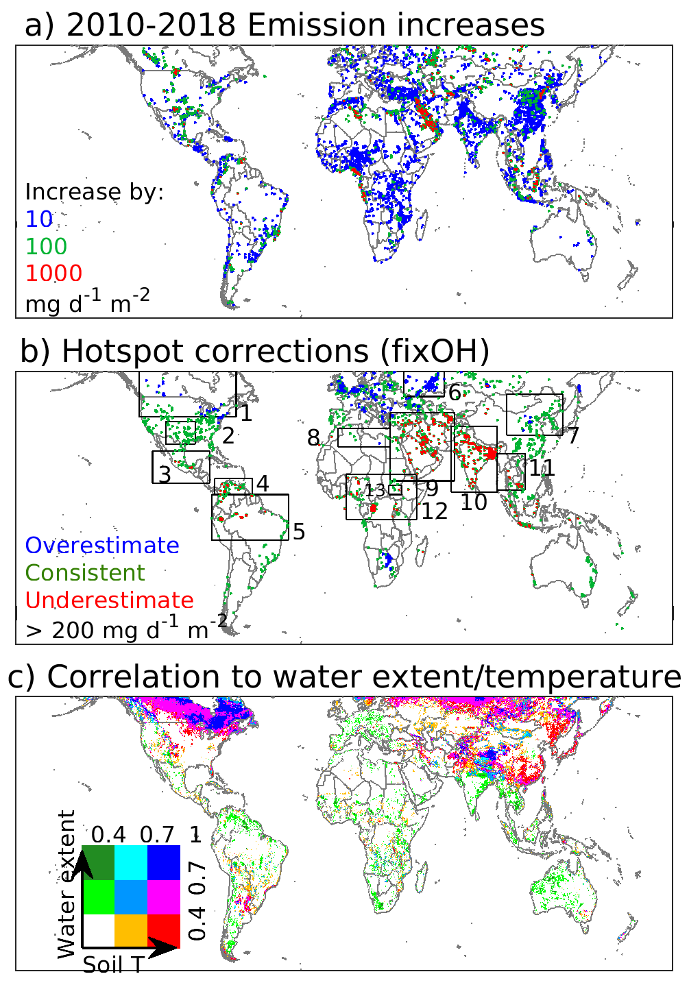
Figure 5(a) Methane emission increases during 2010–2018 estimated from bottom-up information (EDGAR v6, 2022). (b) Methane source hotspots (> 200 kg d−1 km−2) and their TROPOMI-derived emission corrections (blue: > 30 % overestimate; green: accurate to ± 30 %; red: > 30 % underestimate). (c) Correlations between the optimized wetland emissions, soil temperature (0–7 cm; ERA5 2019), and surface water extent (Jensen et al., 2019).
Middle East methane emissions are highly localized, with just 5 % of model grid cells (at 0.1∘ × 0.1∘) accounting for 70 % of the prior regional emissions and 60 % of the derived adjustments. Our multi-model inversion results point to consistent prior underestimates for high emitters in Azerbaijan, Turkmenistan, and Iran, supporting previous satellite-based analyses (Buchwitz et al., 2017; Lauvaux et al., 2022; Schneising et al., 2020; Varon et al., 2019). However, TROPOMI also reveals a large number of hotspots (over Oman, Yemen, Saudi Arabia, Iraq, Turkmenistan, and Iran; Figs. 2a, 5b, and S16) that are entirely missing from the prior inventory. Many of these missing emission hotspots are consistent with facilities on the ground. For example, missing sources in Oman identified through the OG inversion (Figs. S10 and S16) match the location of the Khazzan gas field – one of the Middle East's largest natural gas fields producing ∼ 1–1.5 billion cubic feet per day of natural gas and ∼ 35 000 barrels per day of light oil (NS Energy, 2022). Other detected hotspots correspond to the Masila Basin in Yemen (EIA, 2022), oil fields in Saudi Arabia (e.g., the Ghawar Field, Maps Saudi Arabia, 2022), and super-emitters in Iraq (Lauvaux et al., 2022).
Over northern Africa, TROPOMI identifies large XCH4 enhancements extending from the Libyan coast to Algeria (box 8 in Fig. 2b). These sources are not well represented in the prior inventory but correspond to oil fields in Libya and to part of the Greenstream pipeline system. The OG inversion is partially able to identify these sources, but the attribution is limited to a single 2∘ × 2.5∘ grid cell (Fig. S10).
6.2 Western Russia and North China Plain: an overestimate of fossil fuel emissions
We find from the TROPOMI data that emissions are overestimated in northern Asia, mainly reflecting fossil fuel sources. Specifically, fossil fuel methane emissions are overestimated by 27 % (11 %–40 %) over western Russia (box 6 in Fig. 2b) and by 17 % (1 %–29 %) over the North China Plain (box 7), with these downward corrections reducing the regional model bias to < 6 ppb. The UNFCCC 2016 emissions used a prior account for accidental and intentional methane releases not considered in previous inventories (Scarpelli et al., 2020), leading to a > 2-fold increase over western Russia compared to EDGAR v5. Our results indicate that these emission pathways may be overestimated in UNFCCC 2016 and that the actual fossil fuel methane source from Russia for 2018–2019 lay between the UNFCCC 2016 and EDGAR v5 values. Indeed, subsequent revisions (year 2019; Scarpelli et al., 2022) to the UNFCCC 2016 inventory used here have strongly reduced fossil fuel emission estimates for Russia (e.g., 21 Tg yr−1 from oil in the year 2016 vs. 2 Tg yr−1 in the year 2019) due to updated emission factor assumptions.
Methane emissions in the North China Plain are primarily from coal mines; prior work suggests that these facilities have lower emission factors than in southern China and that their emissions have been declining since 2012 (Sheng et al., 2019). Satellite-based and in situ measurements have pointed to EDGAR v4.3.2 and GFEI emission overestimates for this area (Alexe et al., 2015; Lu et al., 2021; Maasakkers et al., 2019; Monteil et al., 2013; Qu et al., 2021; Turner et al., 2015; Zhang et al., 2021). Here, we use a detailed new inventory for China coal emissions (Sheng et al., 2019) that has > 50 % lower fluxes than EDGAR v4.3.2 over the North China Plain – but find that these are still overestimated. By contrast, upward adjustments are derived over other regions in China such as Xinjiang, where TROPOMI XCH4 enhancements are attributed by the OG and EE inversions to underestimated fossil fuel sources (Fig. S10). Recent work by Lorente et al. (2022) points to some erroneous emission hotspots for this area associated with surface reflectance; we therefore restrict our interpretation here to the regional scale. Positive corrections are also derived for fossil fuel sources in southern China, but their emissions are difficult to isolate from those of nearby rice fields.
6.3 South and Southeast Asia: Major methane emissions during summer monsoon
Methane emissions from South and Southeast Asia are dominated by agriculture (livestock, rice) and waste. The largest emission correction for this area occurs over India, where we find a 23 % (10 %–30 %) underestimate (mainly due to those two sources) and derive total national emissions of 61 [55–64] Tg yr−1. India contains over 35 % and 20 % of the world's cattle and water buffalo, respectively, with both populations increasing over the past decade (Sonavale et al., 2020). Such changes are reflected in both the EDGAR bottom-up inventory (+0.4 Tg yr−1 annual livestock+waste emission increase for 2010–2018, EDGAR v6, 2021) and in analyses based on GOSAT observations (+0.2–0.7 Tg yr−1 inferred annual increase for Indian livestock, Maasakkers et al., 2019; Miller et al., 2019; Zhang et al., 2021). Our inversion for 2018–2019 uses an EDGAR v5 prior estimate for the year 2015, but the inferred +23 % (11 Tg yr−1) correction is too large to be explained solely by intervening trends and thus indicates an emission underestimate for this source.
Over 90 % of the world's rice production occurs in India and Southeast Asia, and we find that the associated methane emissions are underestimated by 39 % (7 %–53 %) and 17 % (7 %–28 %), respectively (boxes 10 and 11 in Fig. 2b). Bottom-up statistics from FAOSTAT (2021) indicate an 8 % increase in crop production over these areas for 2010–2019 due to a 10 % yield increase combined with a 2 % cropland area decrease. Expected emission trends between the timeframe of the EDGAR v5 emissions (2015) and our inversions (2018–2019) can therefore not fully explain the TROPOMI observations, indicating that the prior emissions for this source are too low. The emission corrections mainly occur during the July–October rice growing season that coincides with the summer monsoon. The TROPOMI data reveal several other connections between the East Asian summer monsoon and the regional methane budget, which we explore next based on our monthly downscaled top-down emissions.
Approximately 80 % of India's annual rain falls during the summer monsoon (IPCC, 2021), and across this July–October season we find that methane emissions from the India and Southeast Asia boxes in Fig. 2b are underestimated by 37 % (15 %–45 %). The resulting seasonal flux increase then accounts for over 68 % of the total annual emission correction. While clouds reduce the TROPOMI sampling coverage during this time, we still obtain > 370 000 and > 9000 observations per monsoon season over India and Southeast Asia, respectively, after applying the data quality filters described in Sect. 2.1. The above emission corrections strongly reduce the prior model biases (from −28 to 3 ppb over India and from −41 to −7 ppb over Southeast Asia), with the individual inversions pointing to consistent spatial adjustments. Prior work using GOSAT and in situ measurements has also identified a peak in Indian emissions during July–October that was not well captured by bottom-up predictions (Palmer et al., 2021).
Figure 6 shows that the TROPOMI-derived South Asian emission corrections are spatially and temporally coherent with the summer monsoon onset and withdrawal. Strong upward adjustments are first derived over Bangladesh and East India following monsoon arrival over these areas (early June 2018; late June 2019). As the monsoon advances, the emission corrections then extend more broadly over northern India during July–September. In concert with the monsoon, the upward corrections subsequently withdraw south and east to Bangladesh in October. Only minor emission adjustments are derived for this region outside of the summer monsoon.
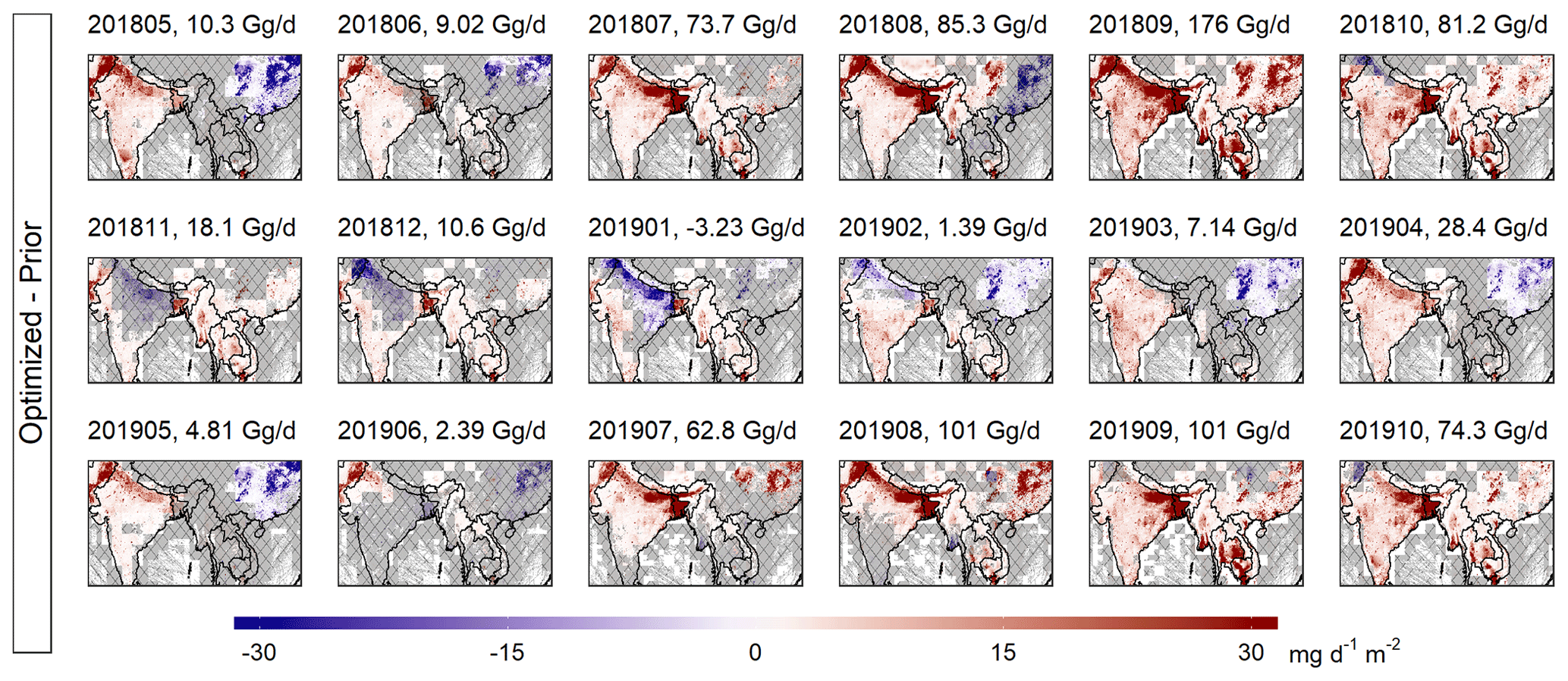
Figure 6TROPOMI-derived emission corrections over South and East Asia based on the fixOH ensemble mean. Shading indicates areas where corrections are not distinguishable from zero (i.e., inversion ensemble includes both positive and negative adjustments).
The above patterns likely reflect hydrologic influences on methane emissions from biotic sources such as wetlands, rice fields, manure, landfills, and sewers. The derived emission corrections exhibit a strong temporal correlation with runoff (R=0.82 in eastern India; R=0.62 in western India), supporting the underlying role of hydrology. Baker et al. (2012) similarly concluded on the basis of aircraft measurements that 64 % of Indian methane emissions during this season reflect monsoon-driven biogenic sources. Increases in Indian summer monsoon precipitation that are projected over the 21st century (Katzenberger et al., 2021) thus raise the strong possibility of enhanced regional methane emissions in the years to come.
6.4 North and South America: increases for fossil fuel sources
We turn next to key oil and gas production fields in North and South America. This includes the US Permian, Barnett, and Eagle Ford region (box 2 in Fig. 5b), previously shown to be the largest US oil- and gas-related methane source (Zhang et al., 2020). Here we infer methane fossil fuel emissions for 2018–2019 that are within 2 % of the prior GEPA estimate. The GEPA estimates are for the year 2016, but based on EDGAR v6 there was no significant regional trend between 2016 and the 2018–2019 inversion period. Over northern Venezuela (box 4 in Fig. 5b), we derive a 28 % (2 %–41 %) upward correction for fossil fuel exploration activities that is consistent across the year, in agreement with the +32 % bottom-up increase for that source that is estimated to have occurred between the prior inventory and inversion timeframes (2016–2018; EDGAR v6, 2021).
Extensive TROPOMI XCH4 enhancements are seen over southern Mexico (Fig. 2b, box 3), and our inversions reveal a 15 % (9 %–25 %) emission underestimate for this area (optimized flux 10 [9–10] Tg yr−1). Trend information from EDGAR v6 (2021) suggests a regional 25 % emission increase for 2016–2020, which could in theory fully explain the derived upward adjustments. However, the observed hotspot locations are largely missing in the prior inventory, and as a result the SF inversion falsely attributes the corrections to upwind waste/landfill sources in Sinaloa. The OG inversion solution aligns more closely with the actual locations of these sources based on the oversampled TROPOMI data (Fig. S10) and is supported by previous regional-scale TROPOMI inversions (Shen et al., 2021) that point to a > 2× emission underestimate of onshore/offshore oil and gas production in the UNFCCC 2016 inventory used here. Aircraft measurements in 2018 also revealed substantial (29 000 kg h−1) methane emissions in the same general region (Zavala-Araiza et al., 2021).
A suite of two-year 4D-Var inversions using satellite-based data from TROPOMI places new constraints on global methane sources. We obtain in this way optimized global emissions of 587 (586–589) Tg yr−1 for 2018–2019. Compared to the most recent GCP estimates (Jackson et al., 2020), our 2018–2019 results point to a larger role for anthropogenic sources, mainly tied to agriculture and waste. We further develop a new framework to map the derived monthly emissions to 0.1∘ × 0.1∘ resolution, enabling the identification of key missing and underestimated sources as highlighted below.
We derive a +24 Tg yr−1 increase in wetland emissions over the prior estimate of 149 Tg yr−1 that mainly (82 %) occurs over the tropics and appears to be related to positive hydrologic anomalies in Amazonia and the Sudd. Meanwhile, fossil fuel emissions in the Middle East are underestimated by 47 % (23 %–57 %) and reached 15.7 (13.2–16.8) Tg yr−1 during our analysis period. Our inversions further uncover missing emission hotspots over Turkmenistan, Iran, Oman, Yemen, Iraq, Libya, Algeria, and Mexico. We estimate long-standing fossil fuel sources in Venezuela at 4.8 (3.8–5.3) Tg yr−1, 28 % (2 %–41 %) higher than the prior estimate (which is for the year 2016).
Inversions point to underestimated agricultural sources in India, the Amazon Basin, central Africa, the US California Central Valley, and Asia. However, more than 45 % (8.5 [3–11] Tg) of the global anthropogenic source adjustment derived here occurs over India and Southeast Asia during the summer monsoon (July–October). We postulate that this reflects the influence of monsoon rainfall on methane emissions from rice, manure, waste, and landfills. Given the projected increase in monsoon precipitation over the coming century (IPCC, 2021), a better understanding of these effects is crucially needed.
Finally, our analyses show that even the dense TROPOMI data coverage does not fully resolve variability in methane sources from that in its sinks. We address the issue in this work by employing validated OH fields from a chemical transport model, but future methane inversions can benefit from incorporating additional datasets (e.g., CO, methyl chloroform, formaldehyde) as constraints on the methane sink (McNorton et al., 2016; Rigby et al., 2017; Turner et al., 2017; Wolfe et al., 2019). Quantitative evaluation of the influence of the 2018–2019 El Niño and the 2021 Hunga Tonga–Hunga Ha'apai eruption on OH variability will also help to advance the accuracy of contemporary methane budget estimates.
TROPOMI data are publicly available online at http://www.tropomi.eu/data-products/level-2-products (Sentinel-5 Precursor/TROPOMI Level 2 Product User Manual: Methane, 2022). TCCON data were obtained from the TCCON Data Archive hosted by CaltechDATA at https://tccondata.org (TCCON, 2014). The GEOS-Chem adjoint code is available at http://adjoint.colorado.edu:8080/gcadj_std.git (last access: 14 February 2023). The modified code used here is archived at https://doi.org/10.13020/g5xc-nj81 (Yu et al., 2021b).
The supplement related to this article is available online at: https://doi.org/10.5194/acp-23-3325-2023-supplement.
XY performed the 4D-Var inversions with help from DBM and DKH. XY, DBM, and DKH designed this study. All authors contributed to the analyses. XY and DBM wrote the manuscript, with comments from all authors.
The contact author has declared that none of the authors has any competing interests.
Publisher’s note: Copernicus Publications remains neutral with regard to jurisdictional claims in published maps and institutional affiliations.
We thank Ilse Aben for assistance with the TROPOMI data; Lee Murray, Benjamin Poulter, Marielle Saunois, and Tia Scarpelli for helpful discussions; and William Brune, David Miller, and Alexander Thames for the ATom OH measurements. We also thank the TCCON, ObsPack, and ATom teams for providing observations used here. This work was supported by NASA's Interdisciplinary Research in Earth Science program (IDS grant no. NNX17AK18G), the US EPA (assistance agreement no. R835873; Center for Air, Climate, and Energy Solutions (CACES)), and the Minnesota Supercomputing Institute. Xueying Yu acknowledges support from a NASA Earth and Space Science Fellowship (grant no. 80NSSC18K1393). Part of this work was carried out at the Jet Propulsion Laboratory, California Institute of Technology, under a contract with the National Aeronautics and Space Administration (NASA). The research has not been formally reviewed by the funders. The views expressed in this document are solely those of the authors and do not necessarily reflect those of the funders. Funders do not endorse any products or commercial services mentioned in this publication.
This research has been supported by the National Aeronautics and Space Administration (grant nos. NNX17AK18G and 80NSSC18K1393) and the U.S. Environmental Protection Agency (grant no. R835873).
This paper was edited by Bryan N. Duncan and reviewed by John Worden and one anonymous referee.
Alexe, M., Bergamaschi, P., Segers, A., Detmers, R., Butz, A., Hasekamp, O., Guerlet, S., Parker, R., Boesch, H., Frankenberg, C., Scheepmaker, R. A., Dlugokencky, E., Sweeney, C., Wofsy, S. C., and Kort, E. A.: Inverse modelling of CH4 emissions for 2010–2011 using different satellite retrieval products from GOSAT and SCIAMACHY, Atmos. Chem. Phys., 15, 113–133, https://doi.org/10.5194/acp-15-113-2015, 2015.
Anderson, D. C., Duncan, B. N., Fiore, A. M., Baublitz, C. B., Follette-Cook, M. B., Nicely, J. M., and Wolfe, G. M.: Spatial and temporal variability in the hydroxyl (OH) radical: understanding the role of large-scale climate features and their influence on OH through its dynamical and photochemical drivers, Atmos. Chem. Phys., 21, 6481–6508, https://doi.org/10.5194/acp-21-6481-2021, 2021.
APEI: Canada's air pollutant emissions inventory, https://open.canada.ca/data/en/dataset/fa1c88a8-bf78-4fcb-9c1e-2a5534b92131, 2020 (last access: 3 March 2023).
Baker, A. K., Schuck, T. J., Brenninkmeijer, C. A. M., Rauthe-Schöch, A., Slemr, F., van Velthoven, P. F. J., and Lelieveld, J.: Estimating the contribution of monsoon-related biogenic production to methane emissions from South Asia using CARIBIC observations, Geophys. Res. Lett., 39, L10813, https://doi.org/10.1029/2012GL051756, 2012.
Barichivich, J., Gloor, E., Peylin, P., Brienen, R. J. W., Schöngart, J., Espinoza, J. C., and Pattnayak, K. C.: Recent intensification of Amazon flooding extremes driven by strengthened Walker circulation, Sci. Adv., 4, eaat8785, https://doi.org/10.1126/sciadv.aat8785, 2018.
Bergamaschi, P., Houweling, S., Segers, A., Krol, M., Frankenberg, C., Scheepmaker, R. A., Dlugokencky, E., Wofsy, S. C., Kort, E. A., Sweeney, C., Schuck, T., Brenninkmeijer, C., Chen, H., Beck, V., and Gerbig, C.: Atmospheric CH4 in the first decade of the 21st century: Inverse modeling analysis using SCIAMACHY satellite retrievals and NOAA surface measurements, J. Geophys. Res.-Atmos., 118, 7350–7369, https://doi.org/10.1002/jgrd.50480, 2013.
Bloom, A. A., Bowman, K. W., Lee, M., Turner, A. J., Schroeder, R., Worden, J. R., Weidner, R., McDonald, K. C., and Jacob, D. J.: A global wetland methane emissions and uncertainty dataset for atmospheric chemical transport models (WetCHARTs version 1.0), Geosci. Model Dev., 10, 2141–2156, https://doi.org/10.5194/gmd-10-2141-2017, 2017.
Bousserez, N., Henze, D. K., Perkins, A., Bowman, K. W., Lee, M., Liu, J., Deng, F., and Jones, D. B. A.: Improved analysis-error covariance matrix for high-dimensional variational inversions: application to source estimation using a 3D atmospheric transport model, Q. J. Roy. Meteor. Soc., 141, 1906–1921, https://doi.org/10.1002/qj.2495, 2015.
Bousserez, N., Henze, D. K., Rooney, B., Perkins, A., Wecht, K. J., Turner, A. J., Natraj, V., and Worden, J. R.: Constraints on methane emissions in North America from future geostationary remote-sensing measurements, Atmos. Chem. Phys., 16, 6175–6190, https://doi.org/10.5194/acp-16-6175-2016, 2016.
BP: British Petroleum Company Limited, https://www.bp.com, last access: 25 April 2022.
Bruhwiler, L., Dlugokencky, E., Masarie, K., Ishizawa, M., Andrews, A., Miller, J., Sweeney, C., Tans, P., and Worthy, D.: CarbonTracker-CH4: an assimilation system for estimating emissions of atmospheric methane, Atmos. Chem. Phys., 14, 8269–8293, https://doi.org/10.5194/acp-14-8269-2014, 2014.
Brune, W. H., Miller, D. O., Thames, A. B., Allen, H. M., Apel, E. C., Blake, D. R., Bui, T. P., Commane, R., Crounse, J. D., Daube, B. C., Diskin, G. S., DiGangi, J. P., Elkins, J. W., Hall, S. R., Hanisco, T. F., Hannun, R. A., Hintsa, E. J., Hornbrook, R. S., Kim, M. J., McKain, K., Moore, F. L., Neuman, J. A., Nicely, J. M., Peischl, J., Ryerson, T. B., St. Clair, J. M., Sweeney, C., Teng, A. P., Thompson, C., Ullmann, K., Veres, P. R., Wennberg, P. O., and Wolfe, G. M.: Exploring oxidation in the remote free troposphere: Insights from Atmospheric Tomography (ATom), J. Geophys. Res.-Atmos., 125, e2019JD031685, https://doi.org/10.1029/2019JD031685, 2020.
Buchwitz, M., Schneising, O., Reuter, M., Heymann, J., Krautwurst, S., Bovensmann, H., Burrows, J. P., Boesch, H., Parker, R. J., Somkuti, P., Detmers, R. G., Hasekamp, O. P., Aben, I., Butz, A., Frankenberg, C., and Turner, A. J.: Satellite-derived methane hotspot emission estimates using a fast data-driven method, Atmos. Chem. Phys., 17, 5751–5774, https://doi.org/10.5194/acp-17-5751-2017, 2017.
Burkholder, J., Sander, S., Abbatt, J., Barker, J., Cappa, C., Crounse, J., Dibble, T., Huie, R., Kolb, C., and Kurylo, M.: Chemical kinetics and photochemical data for use in atmospheric studies, JPL Data Eval., 19, https://jpldataeval.jpl.nasa.gov, 2020.
Chen, H., Karion, A., Rella, C. W., Winderlich, J., Gerbig, C., Filges, A., Newberger, T., Sweeney, C., and Tans, P. P.: Accurate measurements of carbon monoxide in humid air using the cavity ring-down spectroscopy (CRDS) technique, Atmos. Meas. Tech., 6, 1031–1040, https://doi.org/10.5194/amt-6-1031-2013, 2013.
Crippa, M., Guizzardi, D., Muntean, M., Schaaf, E., Lo Vullo, E., Solazzo, E., Monforti-Ferrario, F., Olivier, J., and Vignati, E.: EDGAR v5.0 Greenhouse Gas Emissions, European Commission [data set], https://data.europa.eu/doi/10.2904/JRC_DATASET_EDGAR (last access: 3 March 2023), 2019.
Crippa, M., Solazzo, E., Huang, G., Guizzardi, D., Koffi, E., Muntean, M., Schieberle, C., Friedrich, R., and Janssens-Maenhout, G.: High resolution temporal profiles in the Emissions Database for Global Atmospheric Research, Sci. Data, 7, 1–17, https://doi.org/10.1038/s41597-020-0462-2, 2020.
Cusworth, D. H., Bloom, A. A., Ma, S., Miller, C. E., Bowman, K., Yin, Y., Maasakkers, J. D., Zhang, Y., Scarpelli, T. R., Qu, Z., Jacob, D. J., and Worden, J. R.: A Bayesian framework for deriving sector-based methane emissions from top-down fluxes, Commun. Earth Environ., 2, 1–8, https://doi.org/10.1038/s43247-021-00312-6, 2021.
Darmenov, A. S. and Silva, A. D.: The Quick Fire Emissions Dataset (QFED): Documentation of versions 2.1, 2.2 and 2.4, NASA technical report series on global modeling and data assimilation, NASA TM-2015-104606, Vol. 38, 2015.
EDGAR: EDGAR v5.0 Global Greenhouse Gas Emissions, European Commission [data set], https://edgar.jrc.ec.europa.eu/overview.php?v=50_GHG (last access: 3 March 2023), 2019.
EDGAR: EDGAR v6.0 Global Greenhouse Gas Emissions, European Commission [data set] https://edgar.jrc.ec.europa.eu/dataset_ghg60 (last access: 3 March 2023), 2021.
EIA: US Energy Information Administration Independent Statistics and Analysis, EIA, https://www.eia.gov, last access: 25 April 2022.
ERA5 reanalyses: Copernicus Climate Change Service (C3S) Climate Data Store (CDS), ECMWF [data set], https://cds.climate.copernicus.eu/cdsapp#!/search?text=ERA5 back extension&type=dataset, (last access: 25 April 2022), 2019.
FAOSTAT: Food and Agriculture Organization of the United Nations, FAOSTAT, http://www.fao.org/faostat/en/#data, last access: 25 April 2022.
Franco, B., Mahieu, E., Emmons, L. K., Tzompa-Sosa, Z. A., Fischer, E. V., Sudo, K., Bovy, B., Conway, S., Griffin, D., Hannigan, J. W., Strong, K., and Walker, K. A.: Evaluating ethane and methane emissions associated with the development of oil and natural gas extraction in North America, Environ. Res. Lett., 11, 044010, https://doi.org/10.1088/1748-9326/11/4/044010, 2016.
Frankenberg, C., Aben, I., Bergamaschi, P., Dlugokencky, E. J., van Hees, R., Houweling, S., van der Meer, P., Snel, R., and Tol, P.: Global column-averaged methane mixing ratios from 2003 to 2009 as derived from SCIAMACHY: Trends and variability, J. Geophys. Res.-Atmos., 116, D04302, https://doi.org/10.1029/2010JD014849, 2011.
Fung, I., John, J., Lerner, J., Matthews, E., Prather, M., Steele, L. P., and Fraser, P. J.: Three-dimensional model synthesis of the global methane cycle, J. Geophys. Res.-Atmos., 96, 13033–13065, https://doi.org/10.1029/91jd01247, 1991.
GMAO (Global Modeling and Assimilation Office): GEOS Near-Real Time Data Products, https://gmao.gsfc.nasa.gov/GMAO_products/NRT_products.php (last access: 3 March 2023), 2013.
GOSAT: Greenhouse Gases Observing Satellite, GOSAT, http://www.gosat.nies.go.jp/en/index.html, last access: 25 April 2022.
Gonzalez, A., Millet, D. B., Yu, X., Wells, K. C., Griffis, T. J., Baier, B. C., Campbell, P. C., Choi, Y., DiGangi, J. P., Gvakharia, A., Halliday, H. S., Kort, E. A., McKain, K., Nowak, J. B., and Plant, G.: Fossil versus nonfossil CO sources in the US: New airborne constraints from ACT-America and GEM, Geophys. Res. Lett., 48, e2021GL093361, https://doi.org/10.1029/2021GL093361, 2021.
Heald, C. L., Jacob, D. J., Jones, D. B. A., Palmer, P. I., Logan, J. A., Streets, D. G., Sachse, G. W., Gille, J. C., Hoffman, R. N., and Nehrkorn, T.: Comparative inverse analysis of satellite (MOPITT) and aircraft (TRACE-P) observations to estimate Asian sources of carbon monoxide, J. Geophys. Res.-Atmos., 109, D23306, https://doi.org/10.1029/2004jd005185, 2004.
Henze, D. K., Hakami, A., and Seinfeld, J. H.: Development of the adjoint of GEOS-Chem, Atmos. Chem. Phys., 7, 2413–2433, https://doi.org/10.5194/acp-7-2413-2007, 2007.
Hoesly, R. M., Smith, S. J., Feng, L., Klimont, Z., Janssens-Maenhout, G., Pitkanen, T., Seibert, J. J., Vu, L., Andres, R. J., Bolt, R. M., Bond, T. C., Dawidowski, L., Kholod, N., Kurokawa, J. I., Li, M., Liu, L., Lu, Z., Moura, M. C. P., O'Rourke, P. R., and Zhang, Q.: Historical (1750–2014) anthropogenic emissions of reactive gases and aerosols from the Community Emissions Data System (CEDS), Geosci. Model Dev., 11, 369–408, https://doi.org/10.5194/gmd-11-369-2018, 2018.
Hozo, S. P., Djulbegovic, B., and Hozo, I.: Estimating the mean and variance from the median, range, and the size of a sample, BMC Med. Res. Methodol., 5, 13, https://doi.org/10.1186/1471-2288-5-13, 2005.
Hu, H., Landgraf, J., Detmers, R., Borsdorff, T., Aan de Brugh, J., Aben, I., Butz, A., and Hasekamp, O.: Toward global mapping of methane with TROPOMI: first results and intersatellite comparison to GOSAT, Geophys. Res. Lett., 45, 3682–3689, https://doi.org/10.1002/2018gl077259, 2018.
Hu, H., Hasekamp, O., Butz, A., Galli, A., Landgraf, J., Aan de Brugh, J., Borsdorff, T., Scheepmaker, R., and Aben, I.: The operational methane retrieval algorithm for TROPOMI, Atmos. Meas. Tech., 9, 5423–5440, https://doi.org/10.5194/amt-9-5423-2016, 2016.
Hu, L., Millet, D. B., Baasandorj, M., Griffis, T. J., Turner, P., Helmig, D., Curtis, A. J., and Hueber, J.: Isoprene emissions and impacts over an ecological transition region in the U.S. Upper Midwest inferred from tall tower measurements, J. Geophys. Res.-Atmos., 120, 3553–3571, https://doi.org/10.1002/2014JD022732, 2015.
IPCC: Climate Change 2021: The Physical Science Basis. Contribution of Working Group I to the Sixth Assessment Report of the Intergovernmental Panel on Climate Change, Cambridge University Press, https://doi.org/10.1017/9781009157896, 2021.
Irakulis-Loitxate, I., Gorroño, J., Zavala-Araiza, D., and Guanter, L.: Satellites detect a methane ultra-emission event from an offshore platform in the Gulf of Mexico, Environ. Sci. Technol. Lett., 9, 520–525, https://doi.org/10.1021/acs.estlett.2c00225, 2022.
Jackson, R. B., Saunois, M., Bousquet, P., Canadell, J. G., Poulter, B., Stavert, A. R., Bergamaschi, P., Niwa, Y., Segers, A., and Tsuruta, A.: Increasing anthropogenic methane emissions arise equally from agricultural and fossil fuel sources, Environ. Res. Lett., 15, 071002, https://doi.org/10.1088/1748-9326/ab9ed2, 2020.
Jacob, D. J., Turner, A. J., Maasakkers, J. D., Sheng, J., Sun, K., Liu, X., Chance, K., Aben, I., McKeever, J., and Frankenberg, C.: Satellite observations of atmospheric methane and their value for quantifying methane emissions, Atmos. Chem. Phys., 16, 14371–14396, https://doi.org/10.5194/acp-16-14371-2016, 2016.
Jensen, K. and Mcdonald, K.: Surface water microwave product series version 3: a near-real time and 25-year historical global inundated area fraction time series from active and passive microwave remote sensing, IEEE Geosci. Remote Sens. Lett., 16, 1402–1406, https://doi.org/10.1109/LGRS.2019.2898779, 2019.
Katzenberger, A., Schewe, J., Pongratz, J., and Levermann, A.: Robust increase of Indian monsoon rainfall and its variability under future warming in CMIP6 models, Earth Syst. Dynam., 12, 367–386, https://doi.org/10.5194/esd-12-367-2021, 2021.
Kleinen, T., Mikolajewicz, U., and Brovkin, V.: Terrestrial methane emissions from the Last Glacial Maximum to the preindustrial period, Clim. Past, 16, 575–595, https://doi.org/10.5194/cp-16-575-2020, 2020.
Kort, E. A., Smith, M. L., Murray, L. T., Gvakharia, A., Brandt, A. R., Peischl, J., Ryerson, T. B., Sweeney, C., and Travis, K.: Fugitive emissions from the Bakken shale illustrate role of shale production in global ethane shift, Geophys. Res. Lett., 43, 4617–4623, https://doi.org/10.1002/2016GL068703, 2016.
Koster, R. D., Darmenov, A. S., and da Silva, A. M.: The Quick Fire Emissions Dataset (QFED): Documentation of Versions 2.1, 2.2 and 2.4, Vol. 38, Technical Report Series on Global Modeling and Data Assimilation, https://gmao.gsfc.nasa.gov/pubs/docs/Darmenov796.pdf (last access: 3 March 2022), 2015.
Krol, M. and Lelieveld, J.: Can the variability in tropospheric OH be deduced from measurements of 1,1,1-trichloroethane (methyl chloroform)?, J. Geophys. Res.-Atmos., 108, 4125, https://doi.org/10.1029/2002JD002423, 2003.
Lauvaux, T., Giron, C., Mazzolini, M., d'Aspremont, A., Duren, R., Cusworth, D., Shindell, D., and Ciais, P.: Global assessment of oil and gas methane ultra-emitters, Science, 375, 557–561, https://doi.org/10.1126/science.abj4351, 2022.
Lehner, B. and Döll, P.: Development and validation of a global database of lakes, reservoirs and wetlands, J. Hydrol., 296, 1–22, https://doi.org/10.1016/j.jhydrol.2004.03.028, 2004.
Li, M., Karu, E., Brenninkmeijer, C., Fischer, H., Lelieveld, J., and Williams, J.: Tropospheric OH and stratospheric OH and Cl concentrations determined from CH4, CH3Cl, and SF6 measurements, npj Clim. Atmos. Sci., 1, 29, https://doi.org/10.1038/s41612-018-0041-9, 2018.
Lin, S.-J. and Rood, R. B.: Multidimensional Flux-Form Semi-Lagrangian transport schemes, Mon. Weather Rev., 124, 2046–2070, https://doi.org/10.1175/1520-0493(1996)124<2046:mffslt>2.0.co;2, 1996.
Liu, M., van der A, R., van Weele, M., Eskes, H., Lu, X., Veefkind, P., de Laat, J., Kong, H., Wang, J., Sun, J., Ding, J., Zhao, Y., and Weng, H.: A new divergence method to quantify methane emissions using observations of Sentinel-5P TROPOMI, Geophys. Res. Lett., 48, e2021GL094151, https://doi.org/10.1029/2021GL094151, 2021.
Lorente, A., Borsdorff, T., Butz, A., Hasekamp, O., aan de Brugh, J., Schneider, A., Wu, L., Hase, F., Kivi, R., Wunch, D., Pollard, D. F., Shiomi, K., Deutscher, N. M., Velazco, V. A., Roehl, C. M., Wennberg, P. O., Warneke, T., and Landgraf, J.: Methane retrieved from TROPOMI: improvement of the data product and validation of the first 2 years of measurements, Atmos. Meas. Tech., 14, 665–684, https://doi.org/10.5194/amt-14-665-2021, 2021.
Lorente, A., Borsdorff, T., Martinez-Velarte, M. C., and Landgraf, J.: Accounting for surface reflectance spectral features in TROPOMI methane retrievals, Atmos. Meas. Tech. Discuss. [preprint], https://doi.org/10.5194/amt-2022-255, in review, 2022.
Lu, X., Jacob, D. J., Zhang, Y., Maasakkers, J. D., Sulprizio, M. P., Shen, L., Qu, Z., Scarpelli, T. R., Nesser, H., Yantosca, R. M., Sheng, J., Andrews, A., Parker, R. J., Boesch, H., Bloom, A. A., and Ma, S.: Global methane budget and trend, 2010–2017: complementarity of inverse analyses using in situ (GLOBALVIEWplus CH4 ObsPack) and satellite (GOSAT) observations, Atmos. Chem. Phys., 21, 4637–4657, https://doi.org/10.5194/acp-21-4637-2021, 2021.
Lunt, M. F., Palmer, P. I., Feng, L., Taylor, C. M., Boesch, H., and Parker, R. J.: An increase in methane emissions from tropical Africa between 2010 and 2016 inferred from satellite data, Atmos. Chem. Phys., 19, 14721–14740, https://doi.org/10.5194/acp-19-14721-2019, 2019.
Lunt, M. F., Palmer, P. I., Lorente, A., Borsdorff, T., Landgraf, J., Parker, R. J., and Boesch, H.: Rain-fed pulses of methane from East Africa during 2018–2019 contributed to atmospheric growth rate, Environ. Res. Lett., 16, 024021, https://doi.org/10.1088/1748-9326/abd8fa, 2021.
Ma, S., Worden, J. R., Bloom, A. A., Zhang, Y., Poulter, B., Cusworth, D. H., Yin, Y., Pandey, S., Maasakkers, J. D., Lu, X., Shen, L., Sheng, J., Frankenberg, C., Miller, C. E., and Jacob, D. J.: Satellite constraints on the latitudinal distribution and temperature sensitivity of wetland methane emissions, AGU Adv., 2, e2021AV000408, https://doi.org/10.1029/2021AV000408, 2021.
Maasakkers, J. D., Jacob, D. J., Sulprizio, M. P., Scarpelli, T. R., Nesser, H., Sheng, J. X., Zhang, Y., Hersher, M., Bloom, A. A., Bowman, K. W., Worden, J. R., Janssens-Maenhout, G., and Parker, R. J.: Global distribution of methane emissions, emission trends, and OH concentrations and trends inferred from an inversion of GOSAT satellite data for 2010–2015, Atmos. Chem. Phys., 19, 7859–7881, https://doi.org/10.5194/acp-19-7859-2019, 2019.
Maasakkers, J. D., Jacob, D. J., Sulprizio, M. P., Turner, A. J., Weitz, M., Wirth, T., Hight, C., DeFigueiredo, M., Desai, M., Schmeltz, R., Hockstad, L., Bloom, A. A., Bowman, K. W., Jeong, S., and Fischer, M. L.: Gridded national inventory of U.S. methane emissions, Environ. Sci. Technol., 50, 13123–13133, https://doi.org/10.1021/acs.est.6b02878, 2016.
Maasakkers, J. D., Varon, D. J., Elfarsdóttir, A., McKeever, J., Jervis, D., Mahapatra, G., Pandey, S., Lorente, A., Borsdorff, T., Foorthuis, L. R., Schuit, B. J., Tol, P., van Kempen, T. A., van Hees, R., and Aben, I.: Using satellites to uncover large methane emissions from landfills, Sci. Adv., 8, eabn9683, https://doi.org/10.1126/sciadv.abn9683, 2022.
Maps Saudi Arabia: Saudi Arabia oil fields map, https://maps-saudi-arabia.com/saudi-arabia-oil-fields-map, last access: 25 April 2022.
McNorton, J., Wilson, C., Gloor, M., Parker, R. J., Boesch, H., Feng, W., Hossaini, R., and Chipperfield, M. P.: Attribution of recent increases in atmospheric methane through 3-D inverse modelling, Atmos. Chem. Phys., 18, 18149–18168, https://doi.org/10.5194/acp-18-18149-2018, 2018.
McNorton, J., Chipperfield, M. P., Gloor, M., Wilson, C., Feng, W., Hayman, G. D., Rigby, M., Krummel, P. B., O'Doherty, S., Prinn, R. G., Weiss, R. F., Young, D., Dlugokencky, E., and Montzka, S. A.: Role of OH variability in the stalling of the global atmospheric CH4 growth rate from 1999 to 2006, Atmos. Chem. Phys., 16, 7943–7956, https://doi.org/10.5194/acp-16-7943-2016, 2016.
Miller, S. M., Michalak, A. M., Detmers, R. G., Hasekamp, O. P., Bruhwiler, L. M. P., and Schwietzke, S.: China's coal mine methane regulations have not curbed growing emissions, Nat. Commun., 10, 303, https://doi.org/10.1038/s41467-018-07891-7, 2019.
Monteil, G., Houweling, S., Butz, A., Guerlet, S., Schepers, D., Hasekamp, O., Frankenberg, C., Scheepmaker, R., Aben, I., and Röckmann, T.: Comparison of CH4 inversions based on 15 months of GOSAT and SCIAMACHY observations, J. Geophys. Res.-Atmos., 118, 11807-811823, https://doi.org/10.1002/2013jd019760, 2013.
Montzka, S. A., Krol, M., Dlugokencky, E., Hall, B., Jöckel, P., and Lelieveld, J.: Small interannual variability of global atmospheric hydroxyl, Science, 331, 67–69, https://doi.org/10.1126/science.1197640, 2011.
Moorthi, S. and Suarez, M. J.: Relaxed Arakawa-Schubert, A parameterization of moist convection for general circulation models, Mon. Weather Rev., 120, 978–1002, https://doi.org/10.1175/1520-0493(1992)120<0978:rasapo>2.0.co;2, 1992.
Murray, L. T., Logan, J. A., and Jacob, D. J.: Interannual variability in tropical tropospheric ozone and OH: The role of lightning, J. Geophys. Res.-Atmos., 118, 11468–411480, https://doi.org/10.1002/jgrd.50857, 2013.
Naik, V., Voulgarakis, A., Fiore, A. M., Horowitz, L. W., Lamarque, J. F., Lin, M., Prather, M. J., Young, P. J., Bergmann, D., Cameron-Smith, P. J., Cionni, I., Collins, W. J., Dalsøren, S. B., Doherty, R., Eyring, V., Faluvegi, G., Folberth, G. A., Josse, B., Lee, Y. H., MacKenzie, I. A., Nagashima, T., van Noije, T. P. C., Plummer, D. A., Righi, M., Rumbold, S. T., Skeie, R., Shindell, D. T., Stevenson, D. S., Strode, S., Sudo, K., Szopa, S., and Zeng, G.: Preindustrial to present-day changes in tropospheric hydroxyl radical and methane lifetime from the Atmospheric Chemistry and Climate Model Intercomparison Project (ACCMIP), Atmos. Chem. Phys., 13, 5277–5298, https://doi.org/10.5194/acp-13-5277-2013, 2013.
NEIC (National Emissions Inventory Collaborative): 2016beta emissions modeling platform, IWDW, http://views.cira.colostate.edu/wiki/wiki/10197 (last access: 3 March 2023), 2019.
Nepstad, L. S., Gerber, J. S., Hill, J. D., Dias, L. C. P., Costa, M. H., and West, P. C.: Pathways for recent Cerrado soybean expansion: extending the soy moratorium and implementing integrated crop livestock systems with soybeans, Environ. Res. Lett., 14, 044029, https://doi.org/10.1088/1748-9326/aafb85, 2019.
Nisbet, E. G., Dlugokencky, E. J., Manning, M. R., Lowry, D., Fisher, R. E., France, J. L., Michel, S. E., Miller, J. B., White, J. W. C., Vaughn, B., Bousquet, P., Pyle, J. A., Warwick, N. J., Cain, M., Brownlow, R., Zazzeri, G., Lanoisellé, M., Manning, A. C., Gloor, E., Worthy, D. E. J., Brunke, E.-G., Labuschagne, C., Wolff, E. W., and Ganesan, A. L.: Rising atmospheric methane: 2007–2014 growth and isotopic shift, Global Biogeochem. Cy., 30, 1356–1370, https://doi.org/10.1002/2016GB005406, 2016.
NOAA Global Monitoring Laboratory: https://www.esrl.noaa.gov/gmd, last access: 25 April 2022.
NS Energy: Khazzan Tight Gas Project, https://www.nsenergybusiness.com/projects/khazzan-tight-gas-project-oman, last access: 25 April 2022.
Palmer, P. I., Feng, L., Lunt, M. F., Parker, R. J., Bösch, H., Lan, X., Lorente, A., and Borsdorff, T.: The added value of satellite observations of methane forunderstanding the contemporary methane budget, Philos. T. R. Soc. A, 379, 20210106, https://doi.org/10.1098/rsta.2021.0106, 2021.
Pandey, S., Gautam, R., Houweling, S., van der Gon, H. D., Sadavarte, P., Borsdorff, T., Hasekamp, O., Landgraf, J., Tol, P., van Kempen, T., Hoogeveen, R., van Hees, R., Hamburg, S. P., Maasakkers, J. D., and Aben, I.: Satellite observations reveal extreme methane leakage from a natural gas well blowout, P. Natl. Acad. Sci. USA, 116, 26376–26381, https://doi.org/10.1073/pnas.1908712116, 2019.
Parker, R. J., Wilson, C., Bloom, A. A., Comyn-Platt, E., Hayman, G., McNorton, J., Boesch, H., and Chipperfield, M. P.: Exploring constraints on a wetland methane emission ensemble (WetCHARTs) using GOSAT observations, Biogeosciences, 17, 5669–5691, https://doi.org/10.5194/bg-17-5669-2020, 2020.
Patra, P. K., Krol, M. C., Prinn, R. G., Takigawa, M., Mühle, J., Montzka, S. A., Lal, S., Yamashita, Y., Naus, S., Chandra, N., Weiss, R. F., Krummel, P. B., Fraser, P. J., O'Doherty, S., and Elkins, J. W.: Methyl chloroform continues to constrain the hydroxyl (OH) variability in the troposphere, J. Geophys. Res.-Atmos., 126, e2020JD033862, https://doi.org/10.1029/2020JD033862, 2021.
Peischl, J., Karion, A., Sweeney, C., Kort, E., Smith, M., Brandt, A., Yeskoo, T., Aikin, K., Conley, S., and Gvakharia, A.: Quantifying atmospheric methane emissions from oil and natural gas production in the Bakken shale region of North Dakota, J. Geophys. Res.-Atmos., 121, 6101–6111, 2016.
Peng, S., Lin, X., Thompson, R. L., Xi, Y., Liu, G., Hauglustaine, D., Lan, X., Poulter, B., Ramonet, M., Saunois, M., Yin, Y., Zhang, Z., Zheng, B., and Ciais, P.: Wetland emission and atmospheric sink changes explain methane growth in 2020, Nature, 612, 477–482, https://doi.org/10.1038/s41586-022-05447-w, 2022.
Prather, M. J., Holmes, C. D., and Hsu, J.: Reactive greenhouse gas scenarios: Systematic exploration of uncertainties and the role of atmospheric chemistry, Geophys. Res. Lett., 39, L09803, https://doi.org/10.1029/2012GL051440, 2012.
Prinn, R., Huang, J., Weiss, R., Cunnold, D., Fraser, P., Simmonds, P., McCulloch, A., Harth, C., Salameh, P., and O'doherty, S.: Evidence for substantial variations of atmospheric hydroxyl radicals in the past two decades, Science, 292, 1882–1888, 2001.
Prinn, R. G., Huang, J., Weiss, R. F., Cunnold, D. M., Fraser, P. J., Simmonds, P. G., McCulloch, A., Harth, C., Reimann, S., Salameh, P., O'Doherty, S., Wang, R. H. J., Porter, L. W., Miller, B. R., and Krummel, P. B.: Evidence for variability of atmospheric hydroxyl radicals over the past quarter century, Geophys. Res. Lett., 32, L07809, https://doi.org/10.1029/2004GL022228, 2005.
Qu, Z., Jacob, D. J., Shen, L., Lu, X., Zhang, Y., Scarpelli, T. R., Nesser, H., Sulprizio, M. P., Maasakkers, J. D., Bloom, A. A., Worden, J. R., Parker, R. J., and Delgado, A. L.: Global distribution of methane emissions: a comparative inverse analysis of observations from the TROPOMI and GOSAT satellite instruments, Atmos. Chem. Phys., 21, 14159–14175, https://doi.org/10.5194/acp-21-14159-2021, 2021.
Rigby, M., Montzka, S. A., Prinn, R. G., White, J. W. C., Young, D., O'Doherty, S., Lunt, M. F., Ganesan, A. L., Manning, A. J., Simmonds, P. G., Salameh, P. K., Harth, C. M., Mühle, J., Weiss, R. F., Fraser, P. J., Steele, L. P., Krummel, P. B., McCulloch, A., and Park, S.: Role of atmospheric oxidation in recent methane growth, P. Natl. Acad. Sci. USA, 114, 5373–5377, https://doi.org/10.1073/pnas.1616426114, 2017.
Saunois, M., Stavert, A. R., Poulter, B., Bousquet, P., Canadell, J. G., Jackson, R. B., Raymond, P. A., Dlugokencky, E. J., Houweling, S., Patra, P. K., Ciais, P., Arora, V. K., Bastviken, D., Bergamaschi, P., Blake, D. R., Brailsford, G., Bruhwiler, L., Carlson, K. M., Carrol, M., Castaldi, S., Chandra, N., Crevoisier, C., Crill, P. M., Covey, K., Curry, C. L., Etiope, G., Frankenberg, C., Gedney, N., Hegglin, M. I., Höglund-Isaksson, L., Hugelius, G., Ishizawa, M., Ito, A., Janssens-Maenhout, G., Jensen, K. M., Joos, F., Kleinen, T., Krummel, P. B., Langenfelds, R. L., Laruelle, G. G., Liu, L., Machida, T., Maksyutov, S., McDonald, K. C., McNorton, J., Miller, P. A., Melton, J. R., Morino, I., Müller, J., Murguia-Flores, F., Naik, V., Niwa, Y., Noce, S., O'Doherty, S., Parker, R. J., Peng, C., Peng, S., Peters, G. P., Prigent, C., Prinn, R., Ramonet, M., Regnier, P., Riley, W. J., Rosentreter, J. A., Segers, A., Simpson, I. J., Shi, H., Smith, S. J., Steele, L. P., Thornton, B. F., Tian, H., Tohjima, Y., Tubiello, F. N., Tsuruta, A., Viovy, N., Voulgarakis, A., Weber, T. S., van Weele, M., van der Werf, G. R., Weiss, R. F., Worthy, D., Wunch, D., Yin, Y., Yoshida, Y., Zhang, W., Zhang, Z., Zhao, Y., Zheng, B., Zhu, Q., and Zhuang, Q.: The global methane budget 2000–2017, Earth Syst. Sci. Data, 12, 1561–1623, https://doi.org/10.5194/essd-12-1561-2020, 2020.
Scarpelli, T. R., Jacob, D. J., Maasakkers, J. D., Sulprizio, M. P., Sheng, J. X., Rose, K., Romeo, L., Worden, J. R., and Janssens-Maenhout, G.: A global gridded (0.1∘ × 0.1∘) inventory of methane emissions from oil, gas, and coal exploitation based on national reports to the United Nations Framework Convention on Climate Change, Earth Syst. Sci. Data, 12, 563–575, https://doi.org/10.5194/essd-12-563-2020, 2020.
Scarpelli, T. R., Jacob, D. J., Grossman, S., Lu, X., Qu, Z., Sulprizio, M. P., Zhang, Y., Reuland, F., Gordon, D., and Worden, J. R.: Updated Global Fuel Exploitation Inventory (GFEI) for methane emissions from the oil, gas, and coal sectors: evaluation with inversions of atmospheric methane observations, Atmos. Chem. Phys., 22, 3235–3249, https://doi.org/10.5194/acp-22-3235-2022, 2022.
Schaefer, H., Fletcher, S. E. M., Veidt, C., Lassey, K. R., Brailsford, G. W., Bromley, T. M., Dlugokencky, E. J., Michel, S. E., Miller, J. B., Levin, I., Lowe, D. C., Martin, R. J., Vaughn, B. H., and White, J. W. C.: A 21st-century shift from fossil-fuel to biogenic methane emissions indicated by 13CH4, Science, 352, 80–84, https://doi.org/10.1126/science.aad2705, 2016.
Schneising, O., Buchwitz, M., Reuter, M., Vanselow, S., Bovensmann, H., and Burrows, J. P.: Remote sensing of methane leakage from natural gas and petroleum systems revisited, Atmos. Chem. Phys., 20, 9169–9182, https://doi.org/10.5194/acp-20-9169-2020, 2020.
Sentinel-5 Precursor/TROPOMI Level 2 Product User Manual: Methane [data set]: https://sentinel.esa.int/documents/, last access: 29 November 2022.
Shen, L., Zavala-Araiza, D., Gautam, R., Omara, M., Scarpelli, T., Sheng, J., Sulprizio, M. P., Zhuang, J., Zhang, Y., Qu, Z., Lu, X., Hamburg, S. P., and Jacob, D. J.: Unravelling a large methane emission discrepancy in Mexico using satellite observations, Remote Sens. Environ., 260, 112461, https://doi.org/10.1016/j.rse.2021.112461, 2021.
Sheng, J., Song, S., Zhang, Y., Prinn, R. G., and Janssens-Maenhout, G.: Bottom-Up estimates of coal mine methane emissions in China: a gridded inventory, emission factors, and trends, Environ. Sci. Technol. Lett., 6, 473–478, https://doi.org/10.1021/acs.estlett.9b00294, 2019.
Sheng, J.-X., Jacob, D. J., Maasakkers, J. D., Sulprizio, M. P., Zavala-Araiza, D., and Hamburg, S. P.: A high-resolution (0.1∘ × 0.1∘) inventory of methane emissions from Canadian and Mexican oil and gas systems, Atmos. Environ., 158, 211–215, https://doi.org/10.1016/j.atmosenv.2017.02.036, 2017.
Sheng, J. X., Jacob, D. J., Turner, A. J., Maasakkers, J. D., Benmergui, J., Bloom, A. A., Arndt, C., Gautam, R., Zavala-Araiza, D., Boesch, H., and Parker, R. J.: 2010–2016 methane trends over Canada, the United States, and Mexico observed by the GOSAT satellite: contributions from different source sectors, Atmos. Chem. Phys., 18, 12257–12267, https://doi.org/10.5194/acp-18-12257-2018, 2018.
Sherwen, T., Schmidt, J. A., Evans, M. J., Carpenter, L. J., Großmann, K., Eastham, S. D., Jacob, D. J., Dix, B., Koenig, T. K., Sinreich, R., Ortega, I., Volkamer, R., Saiz-Lopez, A., Prados-Roman, C., Mahajan, A. S., and Ordóñez, C.: Global impacts of tropospheric halogens (Cl, Br, I) on oxidants and composition in GEOS-Chem, Atmos. Chem. Phys., 16, 12239–12271, https://doi.org/10.5194/acp-16-12239-2016, 2016.
Sonavale, K., Shaikh, M., Kadam, M., and Pokharkar, V.: Livestock sector in India: a critical analysis, Asian J. Agr. Extens., 38, 51–62, 2020.
Stevenson, D. S., Derwent, R. G., Wild, O., and Collins, W. J.: COVID-19 lockdown emission reductions have the potential to explain over half of the coincident increase in global atmospheric methane, Atmos. Chem. Phys., 22, 14243–14252, https://doi.org/10.5194/acp-22-14243-2022, 2022.
Sun, K., Zhu, L., Cady-Pereira, K., Chan Miller, C., Chance, K., Clarisse, L., Coheur, P. F., González Abad, G., Huang, G., Liu, X., Van Damme, M., Yang, K., and Zondlo, M.: A physics-based approach to oversample multi-satellite, multispecies observations to a common grid, Atmos. Meas. Tech., 11, 6679–6701, https://doi.org/10.5194/amt-11-6679-2018, 2018.
TCCON: Total Carbon Column Observing Network [data set], https://tccondata.org/2014 (last access: 25 April 2022), 2014.
Turner, A. J., Frankenberg, C., Wennberg, P. O., and Jacob, D. J.: Ambiguity in the causes for decadal trends in atmospheric methane and hydroxyl, P. Natl. Acad. Sci. USA, 114, 5367–5372, https://doi.org/10.1073/pnas.1616020114, 2017.
Turner, A. J., Fung, I., Naik, V., Horowitz, L. W., and Cohen, R. C.: Modulation of hydroxyl variability by ENSO in the absence of external forcing, P. Natl. Acad. Sci. USA, 115, 8931–8936, https://doi.org/10.1073/pnas.1807532115, 2018a.
Turner, A. J., Jacob, D. J., Benmergui, J., Brandman, J., White, L., and Randles, C. A.: Assessing the capability of different satellite observing configurations to resolve the distribution of methane emissions at kilometer scales, Atmos. Chem. Phys., 18, 8265–8278, https://doi.org/10.5194/acp-18-8265-2018, 2018b.
Turner, A. J., Jacob, D. J., Wecht, K. J., Maasakkers, J. D., Lundgren, E., Andrews, A. E., Biraud, S. C., Boesch, H., Bowman, K. W., Deutscher, N. M., Dubey, M. K., Griffith, D. W. T., Hase, F., Kuze, A., Notholt, J., Ohyama, H., Parker, R., Payne, V. H., Sussmann, R., Sweeney, C., Velazco, V. A., Warneke, T., Wennberg, P. O., and Wunch, D.: Estimating global and North American methane emissions with high spatial resolution using GOSAT satellite data, Atmos. Chem. Phys., 15, 7049–7069, https://doi.org/10.5194/acp-15-7049-2015, 2015.
UNFCCC: United Nations Framework Convention on Climate Change, https://unfccc.int, last access: 25 April 2021.
Varon, D. J., McKeever, J., Jervis, D., Maasakkers, J. D., Pandey, S., Houweling, S., Aben, I., Scarpelli, T., and Jacob, D. J.: Satellite discovery of anomalously large methane point sources from oil/gas production, Geophys. Res. Lett., 46, 13507–13516, https://doi.org/10.1029/2019gl083798, 2019.
Wecht, K. J., Jacob, D. J., Frankenberg, C., Jiang, Z., and Blake, D. R.: Mapping of North American methane emissions with high spatial resolution by inversion of SCIAMACHY satellite data, J. Geophys. Res.-Atmos., 119, 7741–7756, https://doi.org/10.1002/2014jd021551, 2014.
Wofsy, S. C., Afshar, S., Allen, H. M., Apel, E., Asher, E. C., Barletta, B., Bent, J., Bian, H., Biggs, B. C., Blake, D. R., Blake, N., Bourgeois, I., Brock, C. A., Brune, W. H., Budney, J. W., Bui, T. P., Butler, A., Campuzano-Jost, P., Chang, C. S., Chin, M., Commane, R., Correa, G., Crounse, J. D., Cullis, P. D., Daube, B. C., Day, D. A., Dean-Day, J. M., Dibb, J. E., Digangi, J. P., Diskin, G. S., Dollner, M., Elkins, J. W., Erdesz, F., Fiore, A. M., Flynn, C. M., Froyd, K., Gesler, D. W., Hall, S. R., Hanisco, T. F., Hannun, R. A., Hills, A. J., Hintsa, E. J., Hoffman, A., Hornbrook, R. S., Huey, L. G., Hughes, S., Jimenez, J. L., Johnson, B. J., Katich, J. M., Keeling, R., Kim, M. J., Kupc, A., Lait, L. R., Lamarque, J. F., Liu, J., McKain, K., McLaughlin, R. J., Meinardi, S., Miller, D. O., Montzka, S. A., Moore, F. L., Morgan, E. J., Murphy, D. M., Murray, L. T., Nault, B. A., Neuman, J. A., Newman, P. A., Nicely, J. M., Pan, X., Paplawsky, W., Peischl, J., Prather, M. J., Price, D. J., Ray, E., Reeves, J. M., Richardson, M., Rollins, A. W., Rosenlof, K. H., Ryerson, T. B., Scheuer, E., Schill, G. P., Schroder, J. C., Schwarz, J. P., St.Clair, J. M., Steenrod, S. D., Stephens, B. B., Strode, S. A., Sweeney, C., Tanner, D., Teng, A. P., Thames, A. B., Thompson, C. R., Ullmann, K., Veres, P. R., Vizenor, N., Wagner, N. L., Watt, A., Weber, R., Weinzierl, B., Wennberg, P., Williamson, C. J., Wilson, J. C., Wolfe, G. M., Woods, C. T., and Zeng, L. H.: ATom: Merged Atmospheric Chemistry, Trace Gases, and Aerosols [data set], https://doi.org/10.3334/ORNLDAAC/1581, 2018.
Wolfe, G. M., Nicely, J. M., St. Clair, J. M., Hanisco, T. F., Liao, J., Oman, L. D., Brune, W. B., Miller, D., Thames, A., González Abad, G., Ryerson, T. B., Thompson, C. R., Peischl, J., McKain, K., Sweeney, C., Wennberg, P. O., Kim, M., Crounse, J. D., Hall, S. R., Ullmann, K., Diskin, G., Bui, P., Chang, C., and Dean-Day, J.: Mapping hydroxyl variability throughout the global remote troposphere via synthesis of airborne and satellite formaldehyde observations, P. Natl. Acad. Sci. USA, 116, 11171–11180, https://doi.org/10.1073/pnas.1821661116, 2019.
Worden, J. R., Cusworth, D. H., Qu, Z., Yin, Y., Zhang, Y., Bloom, A. A., Ma, S., Byrne, B. K., Scarpelli, T., Maasakkers, J. D., Crisp, D., Duren, R., and Jacob, D. J.: The 2019 methane budget and uncertainties at 1∘ resolution and each country through Bayesian integration Of GOSAT total column methane data and a priori inventory estimates, Atmos. Chem. Phys., 22, 6811–6841, https://doi.org/10.5194/acp-22-6811-2022, 2022.
Wu, S., Mickley, L. J., Jacob, D. J., Logan, J. A., Yantosca, R. M., and Rind, D.: Why are there large differences between models in global budgets of tropospheric ozone?, J. Geophys. Res.-Atmos., 112, D05302, https://doi.org/10.1029/2006JD007801, 2007.
Xiao, Y., Logan, J. A., Jacob, D. J., Hudman, R. C., Yantosca, R., and Blake, D. R.: Global budget of ethane and regional constraints on U.S. sources, J. Geophys. Res.-Atmos., 113, D21306, https://doi.org/10.1029/2007jd009415, 2008.
Yu, X., Millet, D. B., and Henze, D. K.: How well can inverse analyses of high-resolution satellite data resolve heterogeneous methane fluxes? Observing system simulation experiments with the GEOS-Chem adjoint model (v35), Geosci. Model Dev., 14, 7775–7793, https://doi.org/10.5194/gmd-14-7775-2021, 2021a.
Yu, X., Millet, D. B., and Henze, D. K.: Code updates of GEOS-Chem Adjoint v35 for TROPOMI methane 4D-Var Inversion, University of Minnesota [code], https://doi.org/10.13020/g5xc-nj81, 2021b.
Yu, X., Millet, D. B., Wells, K. C., Griffis, T. J., Chen, X., Baker, J. M., Conley, S. A., Smith, M. L., Gvakharia, A., Kort, E. A., Plant, G., and Wood, J. D.: Top-Down constraints on methane point source emissions from animal agriculture and waste based on new airborne measurements in the U.S. Upper Midwest, J. Geophys. Res.-Biogeo., 125, e2019JG005429, https://doi.org/10.1029/2019jg005429, 2020.
Yu, X., Millet, D. B., Wells, K. C., Henze, D. K., Cao, H., Griffis, T. J., Kort, E. A., Plant, G., Deventer, M. J., Kolka, R. K., Roman, D. T., Davis, K. J., Desai, A. R., Baier, B. C., McKain, K., Czarnetzki, A. C., and Bloom, A. A.: Aircraft-based inversions quantify the importance of wetlands and livestock for Upper Midwest methane emissions, Atmos. Chem. Phys., 21, 951–971, https://doi.org/10.5194/acp-21-951-2021, 2021c.
Zavala-Araiza, D., Omara, M., Gautam, R., Smith, M. L., Pandey, S., Aben, I., Almanza-Veloz, V., Conley, S., Houweling, S., Kort, E. A., Maasakkers, J. D., Molina, L. T., Pusuluri, A., Scarpelli, T., Schwietzke, S., Shen, L., Zavala, M., and Hamburg, S. P.: A tale of two regions: methane emissions from oil and gas production in offshore/onshore Mexico, Environ. Res. Lett., 16, 024019, https://doi.org/10.1088/1748-9326/abceeb, 2021.
Zhang, Y., Jacob, D. J., Maasakkers, J. D., Sulprizio, M. P., Sheng, J. X., Gautam, R., and Worden, J.: Monitoring global tropospheric OH concentrations using satellite observations of atmospheric methane, Atmos. Chem. Phys., 18, 15959–15973, https://doi.org/10.5194/acp-18-15959-2018, 2018.
Zhang, Y., Jacob, D. J., Lu, X., Maasakkers, J. D., Scarpelli, T. R., Sheng, J. X., Shen, L., Qu, Z., Sulprizio, M. P., Chang, J., Bloom, A. A., Ma, S., Worden, J., Parker, R. J., and Boesch, H.: Attribution of the accelerating increase in atmospheric methane during 2010–2018 by inverse analysis of GOSAT observations, Atmos. Chem. Phys., 21, 3643–3666, https://doi.org/10.5194/acp-21-3643-2021, 2021.
Zhang, Y., Gautam, R., Pandey, S., Omara, M., Maasakkers, J. D., Sadavarte, P., Lyon, D., Nesser, H., Sulprizio, M. P., Varon, D. J., Zhang, R., Houweling, S., Zavala-Araiza, D., Alvarez, R. A., Lorente, A., Hamburg, S. P., Aben, I., and Jacob, D. J.: Quantifying methane emissions from the largest oil-producing basin in the United States from space, Sci. Adv., 6, eaaz5120, https://doi.org/10.1126/sciadv.aaz5120, 2020.
Zhao, Y., Saunois, M., Bousquet, P., Lin, X., Berchet, A., Hegglin, M. I., Canadell, J. G., Jackson, R. B., Hauglustaine, D. A., Szopa, S., Stavert, A. R., Abraham, N. L., Archibald, A. T., Bekki, S., Deushi, M., Jöckel, P., Josse, B., Kinnison, D., Kirner, O., Marécal, V., O'Connor, F. M., Plummer, D. A., Revell, L. E., Rozanov, E., Stenke, A., Strode, S., Tilmes, S., Dlugokencky, E. J., and Zheng, B.: Inter-model comparison of global hydroxyl radical (OH) distributions and their impact on atmospheric methane over the 2000–2016 period, Atmos. Chem. Phys., 19, 13701–13723, https://doi.org/10.5194/acp-19-13701-2019, 2019.
- Abstract
- Introduction
- Data and methods
- Derived global methane budget and sensitivity to OH
- Global methane sources and top emitting countries
- Wetland sources are underestimated in the tropics
- Anthropogenic sources and emission hotspots
- Conclusions
- Code and data availability
- Author contributions
- Competing interests
- Disclaimer
- Acknowledgements
- Financial support
- Review statement
- References
- Supplement