the Creative Commons Attribution 4.0 License.
the Creative Commons Attribution 4.0 License.
 | 09 Mar 2023
Impacts of estimated plume rise on PM2.5 exceedance prediction during extreme wildfire events: a comparison of three schemes (Briggs, Freitas, and Sofiev)
Siqi Ma
Saulo R. Freitas
Ravan Ahmadov
Mikhail Sofiev
Xiaoyang Zhang
Shobha Kondragunta
Ralph Kahn
Youhua Tang
Barry Baker
Patrick Campbell
Rick Saylor
Georg Grell
Fangjun Li
Plume height plays a vital role in wildfire smoke dispersion and the subsequent effects on air quality and human health. In this study, we assess the impact of different plume rise schemes on predicting the dispersion of wildfire air pollution and the exceedances of the National Ambient Air Quality Standards (NAAQS) for fine particulate matter (PM2.5) during the 2020 western United States wildfire season. Three widely used plume rise schemes (Briggs, 1969; Freitas et al., 2007; Sofiev et al., 2012) are compared within the Community Multiscale Air Quality (CMAQ) modeling framework. The plume heights simulated by these schemes are comparable to the aerosol height observed by the Multi-angle Imaging SpectroRadiometer (MISR) and Cloud-Aerosol Lidar and Infrared Pathfinder Satellite Observations (CALIPSO). The performance of the simulations with these schemes varies by fire case and weather conditions. On average, simulations with higher plume injection heights predict lower aerosol optical depth (AOD) and surface PM2.5 concentrations near the source region but higher AOD and PM2.5 in downwind regions due to the faster spread of the smoke plume once ejected. The 2-month mean AOD difference caused by different plume rise schemes is approximately 20 %–30 % near the source regions and 5 %–10 % in the downwind regions. Thick smoke blocks sunlight and suppresses photochemical reactions in areas with high AOD. The surface PM2.5 difference reaches 70 % on the West Coast of the USA, and the difference is lower than 15 % in the downwind regions. Moreover, the plume injection height affects pollution exceedance (>35 µg m−3) predictions. Higher plume heights generally produce larger downwind PM2.5 exceedance areas. The PM2.5 exceedance areas predicted by the three schemes largely overlap, suggesting that all schemes perform similarly during large wildfire events when the predicted concentrations are well above the exceedance threshold. At the edges of the smoke plumes, however, there are noticeable differences in the PM2.5 concentration and predicted PM2.5 exceedance region. For the whole period of study, the difference in the total number of exceedance days could be as large as 20 d in northern California and 4 d in the downwind regions. This disagreement among the PM2.5 exceedance forecasts may affect key decision-making regarding early warning of extreme air pollution episodes at local levels during large wildfire events.
- Article
(11306 KB) - Full-text XML
- BibTeX
- EndNote


Wildfires release large amounts of aerosol and trace gases into the atmosphere, which degrades the air quality and adversely affects human health (Koning et al., 1985). Previous studies (Reid et al., 2016; Cascio, 2018) have demonstrated that a strong association exists between exposure to wildfire smoke and all-cause mortality and respiratory morbidity. The global average mortality attributable to landscape fire smoke exposure was estimated at 339 000 deaths annually (Johnston et al., 2012). O'Neill et al. (2021) discuss the regional health impacts of the 2017 northern California wildfires and estimated 83 excess deaths from exposure to PM2.5 (i.e., particles having aerodynamic diameter of less than 2.5 µm), of which 47 % were attributable to wildfire smoke during the smoke episode. Liu et al. (2021) assessed the health impact of the 2020 Washington State wildfire smoke episode, which caused 38.4 more all-cause mortality cases and 15.1 more respiratory mortality cases. Aerosols emitted from wildfires also affect the photolysis rates and photochemistry (Tang et al., 2003) and ozone photochemical production (Val Martin et al., 2006; Akagi et al., 2013). Wilmot et al. (2022) produced a decadal-scale wildfire plume rise climatology for the USA West Coast and Canada and found trends toward enhanced plume heights and surface smoke injection to the free troposphere, which suggest a growing impact of wildfires on air quality and regional climate.
Previous studies have found that the smoke injection height plays a vital role in smoke dispersion, as wind speed and direction generally vary with altitude (e.g., Mallia et al., 2018; Vernon et al., 2018). In addition, a higher injection height will reduce near-source concentration, increase downwind concentrations (Li et al., 2020), and can influence the removal processes and atmospheric lifetime of emitted particles and trace gases. Briggs (1969) introduced a set of semi-empirical formulas to estimate plume injection height for stack emissions from stationary power plant point sources in different atmospheric stability states using buoyancy flux, horizontal wind speed, static stability, and atmospheric turbulence conditions. This scheme is widely used in dispersion models such as the National Oceanic and Atmospheric Administration (NOAA) Hybrid Single-Particle Lagrangian Integrated Trajectory model (HYSPLIT; Draxler and Hess, 1998) and Community Multiscale Air Quality Modeling System (CMAQ; Byun and Schere, 2006). However, the Briggs scheme was not designed for irregular-occurrence, large point source emissions, such as forest fires. Also, some of the input parameters, such as heat flux, are difficult to obtain. Freitas et al. (2007) developed a 1-D plume rise and transport parameterization for low-resolution atmospheric chemistry models, which was built upon governing equations, for the first law of thermodynamics, vertical motion, and continuity for the water phases. Sofiev et al. (2012) developed a new plume rise scheme, which utilizes the fire radiative power (FRP), planetary boundary layer (PBL) height, and the Brunt–Vaisala frequency in the free troposphere to estimate the plume injection height from wildfires. The parameters of the new scheme were determined using the plume height observations collected by the Multi-angle Imaging SpectroRadiometer (MISR) Plume Height Project (Kahn et al., 2008; Mazzoni et al., 2007) in North America (Val Martin et al., 2010) and Siberia. The plume height estimation in models is of great uncertainty. Sessions et al. (2011) tested the Freitas et al. (2007) plume rise scheme with Weather Research and Forecasting model coupled with Chemistry (WRF-Chem) and found that differences in injection heights produce different transport pathways. Roy et al. (2017) compared the simulated plume heights from two different approaches, namely Western Regional Air Partnership's (WRAP) plume model and the Freitas et al. (2007) plume model. Results show that the Freitas et al. (2007) plume model had a better diurnal variation in the plume rise height. Mallia et al. (2018) tested different ways to distribute the fire emissions vertically for prescribed fires. Results indicated that plume height plays a critical role in determining how smoke distributes downwind of the fire. Ye et al. (2021) compared the calculated plume heights from 12 state-of-the-art air quality forecasting systems during the Williams Flats fire in Washington State, USA, in August 2019, during the Fire Influence on Regional to Global Environments and Air Quality (FIREX-AQ) field campaign. They found that there was a large spread of the modeled plume heights.
In the summer and early autumn of 2020, the western United States (USA) experienced a record-breaking wildfire season. A series of large wildfires fueled by accumulated biomass, heat waves, and dry winds burned more than 10 ×106 acres (National Interagency Fire Center, 2020). From late August to early October 2020, the West Coast wildfires contributed 23 % of surface PM2.5 pollution nationwide and caused 3720 observed PM2.5 exceedances (daily PM2.5>35 µg m−3, based on National Ambient Air Quality Standards – NAAQS; Li et al., 2021). The thick fire smoke that originated in California, Oregon, and Washington was injected into the free troposphere and transported across the country by the prevailing wind, which caused hazy days (indicated by the high-aerosol-optical-depth (AOD) region) in 19 states (Fig. 1).
This study aims to evaluate the impact of different plume rise schemes on aerosol distribution and photochemistry during the 2020 record-breaking wildfire season. We use the George Mason University (GMU) wildfire forecast system (Li et al., 2021) that relies on satellite estimates of biomass burning emissions and CMAQ to simulate the emission, transport, and transformation of smoke during the 2020 summer wildfire season. Three plume rise schemes are used, namely Briggs (1969), Freitas et al. (2007), and Sofiev et al. (2012). The Briggs (1969) scheme was implemented in the standard release of the CMAQ version. Li et al. (2021) implemented the Sofiev et al. (2012) scheme into CMAQ, and in this work, the Freitas et al. (2007) scheme is also implemented. The plume injection height's impact on PM2.5 vertical distribution is evaluated in Sect. 3.2. Its impact on AOD and photochemistry is discussed in Sect. 3.3. Finally, we discussed plume rise impact on surface pollution level and PM2.5 exceedance in Sect. 3.4.
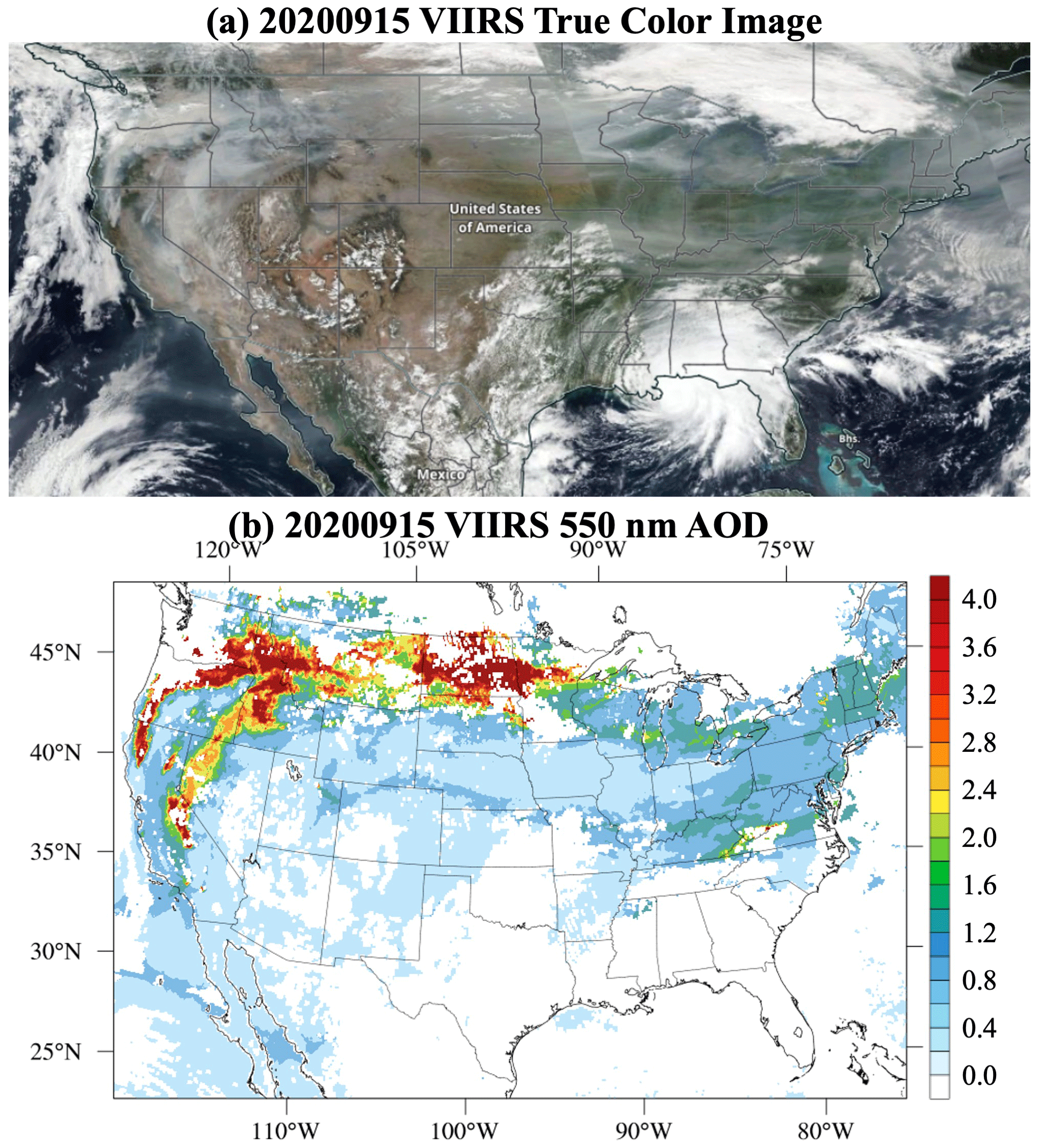
Figure 1Observations of wildfire smoke on 15 September 2020, over the continental United States by the Visible Infrared Imaging Radiometer Suite (VIIRS) aboard the Suomi National Polar-orbiting Partnership (Suomi NPP) satellite. (a) True-color image and (b) 550 nm aerosol optical depth (AOD).
2.1 Experiment design
Biomass burning is an important source of global aerosols that has a great impact on air quality. Figure 2 shows how wildfire smoke affects local and downwind air quality (Koppmann et al., 2005; Seinfeld and Pandis, 2016; Schlosser et al., 2017). Wildfire emissions include primary aerosols (direct emission) and large amounts of gases that can be oxidized to form secondary aerosols (generated after emission). In the biomass burning input of our model, the major components of the primary aerosols are organic carbon, non-carbon organic matter, elemental carbon, chloride, and potassium. The other wildfire emissions like SO2, NOx (NO + NO2), NH3, and volatile organic compounds (VOCs) may form secondary aerosols such as sulfate, nitrate, ammonium, and secondary organic aerosols (SOAs) after being emitted. The temporal and spatial impacts of plume rise on different primary or secondary aerosol species may be different, as the generation of the secondary aerosols usually takes time. The difference in the dispersion of primary and secondary aerosols will contribute to further differences in photochemistry and health impacts. Therefore, it is important to discuss the impact of plume rise on each primary and secondary aerosol species.
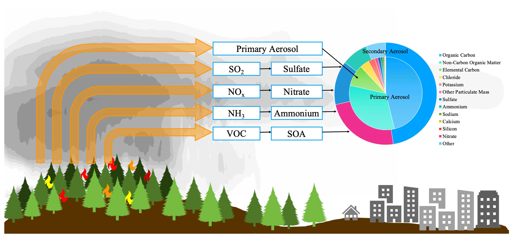
Figure 2Wildfire primary emissions and downwind evolution. Note that the percentage for primary aerosols is from the CMAQ biomass burning input file. The percentage for the secondary aerosols is not real; it is just for illustration purposes. Moreover, the CMAQ model separates organic carbon (OC) and non-carbon elements (O, H, etc.) in organic matter (OM).
To evaluate the impact of different plume rise schemes on aerosol dispersion and photochemistry modeling during the 2020 record-breaking wildfire season, four CMAQ simulations were conducted. In the first run (B69), we used the CMAQ default plume rise scheme based on Briggs (1969). In the second run (F07), we implemented the Freitas et al. (2007) scheme into the CMAQ model and used it to calculate the plume injection height. In the third run (S12), we used the Sofiev et al. (2012) plume rise scheme, as implemented in Li et al. (2021). In the fourth run (NoFire), we turned off all types of biomass burning emissions. The wildfire impact is represented by the difference between the simulation with fire and the NoFire run. More information on the three plume rise schemes is provided in Sect. 2.3. Besides the difference in the plume rise scheme, the setups for these three runs are the same. More details about the CMAQ setup are given in Sect. 2.2. Comparing results from these three simulations elucidates the impacts of plume injection height predictions on the distribution of each aerosol species (Sect. 3.2), AOD, and photochemistry (Sect. 3.3), as well as surface air quality and PM2.5 exceedances (Sect. 3.4).
2.2 Description of the model system
The George Mason University (GMU) air quality modeling system was employed to simulate the 2020 summer wildfire season from 1 August to 30 September 2020 over the contiguous United States (CONUS) domain. This system uses CMAQ version 5.3.1 (United States Environmental Protection Agency, 2020a) as the chemical transport model and the Weather Research and Forecasting (WRF; Skamarock et al., 2019) model (Version 4.2 output) as the meteorology inputs for the CMAQ model. The model domain is configured with 12 km by 12 km horizontal resolution and 35 vertical layers (the same horizontal and vertical resolution as NOAA's operational National Air Quality Forecasting Capability). The initial and boundary conditions for WRF are from the Global Data Assimilation System (GDAS) 0.25∘ analysis and forecast. The main physics choices were the Grell–Freitas scheme (Grell and Freitas, 2014) for parameterized cumulus processes, the Mellor–Yamada–Janjic scheme (Janjic, 1994) for planetary boundary layer (PBL) processes, the two-moment Morrison microphysics (Morrison et al., 2009) for cloud physics processes, the rapid radiative transfer model for general circulation models (RRTMG) scheme (Iacono et al., 2008) for longwave and shortwave radiation, and the Noah scheme (Koren et al., 1999) for land surface processes. The biomass burning emissions product used in this study is the 0.1∘ daily blended Global Biomass Burning Emissions Product (GBBEPx) from the Moderate Resolution Imaging Spectroradiometer (MODIS) and Visible Infrared Imaging Radiometer Suite (VIIRS; GBBEPx V3; Zhang et al., 2012, 2019). The GBBEPx fire radiative power (FRP) in the GBBEPx is averaged from observations from MODIS on Terra and Aqua MODIS and VIIRS M band on the Suomi National Polar-orbiting Partnership (SNPP) and the Joint Polar Satellite System-1 (JPSS) VIIRS. A climatological diurnal cycle from the Western Regional Air Partnership (WRAP) work was applied to the daily GBBEPx emission to derive hourly model-ready emission input. Anthropogenic emissions were prepared with the 2016v1 emissions modeling platform, using the baseline emissions taken from the National Emissions Inventory (NEI) 2016 collaboration (Eyth et al., 2021). We then shifted the base year emission to the prediction year 2020 using representative days of each month. The model-ready emission files are processed and generated by the Sparse Matrix Operator Kernel Emissions (SMOKE) model (Baek and Seppanen, 2019) V4.7. The carbon bond 6 (CB6) gas-phase chemical mechanism (Luecken et al., 2019), CMAQ aerosol module 7 (AE07) aerosol scheme (Pye et al., 2015; Xu et al., 2018), and aqueous chemistry (Fahey et al., 2017) are used in the CMAQ system. Details about the system setup are shown in Table S1 of Li et al. (2021).
The evaluation of the model performance with the Sofiev et al. (2012) plume rise scheme has been discussed by Li et al. (2021). The average correlation between observed (from AirNow) and simulated daily PM2.5 concentrations is 0.55. The averaged normalized mean error in the simulated surface PM2.5 is 3.9 % for the year 2020. The average area hit ratio for exceedances is 0.68 (Fig. 2a in Li et al., 2021). A high area hit ratio represents a good capture of the region impacted by smoke. During the peak pollution days (from 12 to 16 September), the area hit ratios were higher than 0.96, with a maximum of 1.0 on 13 September 2020. This suggests that the model could predict more than 96 % of the observed exceedances when the smoke pollution was at its peak. Also, the simulated PM2.5 vertical profiles along the West Coast and in central USA matched the vertical profiles of backscatter from Cloud-Aerosol Lidar and Infrared Pathfinder Satellite Observations (CALIPSO) near the wildfire source region and downwind area (Fig. S2 in Li et al., 2021). Overall, the model can reproduce wildfire smoke dispersion, especially when the smoke is thick.
2.3 Description of the plume rise schemes
Three plume rise schemes are used in this study, namely Briggs (1969), Freitas et al. (2007), and Sofiev et al. (2012).
2.3.1 Briggs scheme (B69)
The default plume rise scheme in CMAQ is based on Briggs (1969) and has been modified by revisions in Briggs (1971, 1972, 1984). It uses a set of semi-empirical formulas to estimate plume injection height (Hp) in different atmospheric stability states (i.e., neutral, stable, and unstable). Heat flux (B), horizontal wind speed (U), static stability (S), and friction velocity (x∗) are used to estimate the plume injection height as follows:
Previous studies found that FRP is about 10 %–20 % of the total fire heat (Wooster et al., 2005; Freeborn et al., 2008). In this study, we derive the heat flux from FRP provided by the GBBEPx dataset multiplied by a factor of 10, following Val Martin et al. (2012). The Briggs (1969) scheme is widely used in chemical transport models; however, it was not designed for forest fires.
2.3.2 Freitas et al. (2007) scheme (F06)
Freitas et al. (2007) developed a 1-D plume rise and transport parameterization for low-resolution atmospheric chemistry models, which was built upon governing equations for the first law of thermodynamics, vertical motion, and continuity for the water phases (Eqs. 1–5 in Freitas et al., 2007). It takes in fire information, including fire area and heat flux, in addition to atmospheric profile information, including temperature, moisture, density, and wind velocity. The plume-top height is defined as the altitude at which the plume is neutrally buoyant and is approximated as a vertical velocity < 1 m s−1. The Freitas et al. (2007) scheme is the default plume rise scheme in WRF-Chem and has been widely used in many studies (e.g., Sessions et al., 2011; Val Martin et al., 2012; Roy et al., 2017; Mallia et al., 2018). However, the Freitas et al. (2007) scheme has never before been used with CMAQ. In this work, the FRP-based Freitas et al. (2007) scheme from High-Resolution Rapid Refresh coupled with Smoke (HRRR–Smoke; Ahmadov et al., 2017) model has been implemented into CMAQ. Wind, temperature, pressure, and humidity from WRFV4.2 meteorology inputs, as well as FRP and fire burning area, are used to calculate the plume injection height in the model. The FRP from GBBEPx and fire size from RAP–Chem (Rapid Refresh with Chemistry; Archer-Nicholls et al., 2015) are used to calculate fire buoyancy in the model.
2.3.3 Sofiev et al. (2012) scheme (S12)
Sofiev et al. (2012) developed a new plume rise scheme that considers wildfire plumes in a way similar to convective available potential energy (CAPE) computations. It utilizes FRP, PBL height (HPBL), and the Brunt–Vaisala frequency in the free troposphere (BVFT) to estimate the plume injection height from wildfires as follows:
where FRP0 is the reference fire radiative power, which equals 106 W, BV0 is the reference Brunt–Vaisala frequency, which equals s−2, and α, β, γ, δ are constants. In our previous study, we added the Sofiev et al. (2012) scheme to CMAQ (Li et al., 2021) and applied it to predict air quality during the 2020 wildfire season with the same constants found in Sofiev et al. (2012).
After obtaining the estimated plume injection height from the three schemes, the fire emissions were distributed between 0.5–1.5 times the plume injection height (default setting in CMAQ). The three schemes used in the current experiment are very different in their nature and underlying assumptions, but they all were developed with an individual fire as a model source of buoyancy and smoke. In this experiment, and in many other applications of these schemes, the input fire information is gridded with a grid cell size of several kilometers or larger. Strictly speaking, such a setup goes beyond the area of applicability of these schemes. However, with a growing number of gridded fire emission products and their applications for atmospheric composition and air quality tasks, it is important to evaluate this very setup – and to compare the robustness of these models to the violation of their underlying assumptions. In this study, we use the default coefficient settings in each scheme. We did not tune the coefficient of any scheme to obtain the best simulation for any major fire case. The main focus of this study is to evaluate the impact of different plume injection heights on the near-source and downwind air quality, and the 2-month average state is more important to our results and future health studies.
2.4 Observation data
2.4.1 MISR and CALIPSO plume height observation
The predicted plume height is evaluated using observations from Multi-angle Imaging SpectroRadiometer (MISR) and Cloud-Aerosol Lidar and Infrared Pathfinder Satellite Observations (CALIPSO). The MISR instrument obtains imagery of each location within its 380 km wide swath at nine viewing angles, ranging from 70∘ forward, through the nadir, to 70∘ aft, along the orbit track, in each of four spectral bands centered at 446 (blue), 558 (green), 672 (red), and 866 nm (near-infrared) wavelengths (Diner et al., 1998). MISR is in a sun-synchronous orbit, crossing the Equator at approximately 10:30 local time (LT), so observations in the study region occurred in the mid-to-late morning, The MISR INteractive eXplorer (MINX) software is used in this study to derive plume heights from MISR imagery (Nelson et al., 2013; Val Martin et al., 2018). The MINX wind-corrected plume height information is then used to evaluate the simulated plume height in this paper.
CALIPSO is an Earth science observation mission that was launched on 28 April 2006 and flies in a nominal orbital altitude of 705 km and an inclination of 98∘, as part of a constellation of Earth-observing satellites. CALIPSO's lidar instrument, the Cloud-Aerosol Lidar with Orthogonal Polarization (CALIOP), provides high-resolution vertical profiles of aerosol and cloud-attenuated-backscatter signals at 532 and 1064 nm (Winker et al., 2007). The footprint of the lidar beam has a 100 m cross section, with an overpass around 13:30 LT. The CALIPSO smoke injection heights are directly calculated from level 1 attenuated-backscatter profiles at 532 nm, following Amiridis et al. (2010). There are several steps involved in this process. First, GBBEPx FRP data were used to locate the fire location along the CALIPSO swath. Then, a slope method (Pal et al., 1992) is applied to each profile to smooth out the original level 1 532 nm attenuated-backscatter-coefficient profiles at each fire point. Next, we calculate the steep gradient in the attenuated-backscatter profiles. The height of the minimum gradient value is selected as the smoke injection height.
2.4.2 AirNow surface PM2.5 data
The hourly ground PM2.5 observations from the U.S. EPA AirNow network are used to evaluate the surface air pollution predictions in this study. The real-time AirNow measurements are collected by the state, local, or tribal environmental agencies either using federal references or equivalent monitoring methods approved by EPA. The measurements contain air quality data for more than 500 cities across the USA, Canada, and Mexico.
2.4.3 VIIRS AOD data
The simulated AOD results are compared to the VIIRS Enterprise AOD from SNPP (Zhang et al., 2016; Laszlo and Liu, 2022). The VIIRS Enterprise Aerosol Algorithm retrieves AOD at the 750 m pixel level for the nominal wavelength of 550 nm, using radiances from 11 VIIRS channels (412, 445, 488, 555, 672, 746, 865, 1240, 1378, 1610, and 2250 nm). The AOD is calculated separately for land and ocean, using a lookup table of precomputed values for several atmospheric parameters to simplify radiative transfer calculations.
3.1 Comparing simulated plume heights against MISR and CALIPSO observations
The simulated plume heights from three simulations, i.e., B69, F07, and S12, are compared with MISR observations for the Milepost 21 fire on 15 August 2020 and the August Complex fire on 31 August 2020 (Fig. 3) at the MISR local overpass time of around 19:00 UTC. The smoke heights from the model 3-D fields were interpolated to the MISR observation pixels using the nearest-neighbor approach. The performance of different schemes varies by fire cases and weather conditions. For the Milepost 21 fire, the plume heights simulated by B69 and S12 are similar but 25 % and 3 % lower than that by F07 for the easterly and westerly plume. In the case of the August Complex fire northerly plume, the plume heights simulated by S12 are 4 % and 8 % higher than that by B69 and F07, respectively. For the southerly plume, the plume heights simulated by B69 are 16 % and 5 % higher than that by F07 and S12. The simulated PBL heights are displayed in Fig. 3 as a reference. When the fire injection height is lower than the PBL height, then the pollution could become confined to the PBL (Sofiev et al., 2012; Thapa et al., 2022). However, when the plume height is higher than PBL, then the fire smoke can be dispersed into the free troposphere where wind speeds are stronger, leading to a wider range of pollution dispersion. In all four cases analyzed in Fig. 3, the simulated plume heights from the three schemes surpassed the model PBL. Previous studies found that, for large fires that are injected above the PBL, the plume height calculated by S12 is less sensitive to FRP than that calculated by B69 (Li et al., 2020). Some of the fire points during the August Complex fire had higher FRP than that during the Milepost 21 fire, so the estimated plume height by B69 is higher than that by S12. For the F07 scheme, the plume injection height is higher when it is wetter (Freitas et al., 2007). The water vapor mixing ratio on 15 August is higher than on 31 August, which contributes to the higher plume height during the Milepost 21 fire than during the August Complex fire. According to the box-and-whisker chart shown in the right panel of Fig. 3, the simulated plume heights are all within the range of MISR observation. Overall, the simulated plume heights with all three schemes are reasonably comparable to the MISR observations.

Figure 3MISR plume heights superposed on the MODIS Terra visible images (a–d) and the comparisons of the observed plume height with the simulated plume heights (e–h) for the 15 August Milepost 21 fire easterly plume (a, e) and westerly plume (b, f) and the 31 August Complex fire northerly plume (c, g) and southerly plume (d, h). Source: MISR Active Aerosol Plume-Height (AAP) Project, with Ralph A. Kahn, Katherine J. Noyes, James Limbacher (NASA Goddard Space Flight Center), Abigail Nastan (JPL-Caltech), Jason Tackett, and Jean-Paul Vernier (NASA Langley Research Center).
The vertical profiles of CMAQ-simulated PM2.5 are also compared to the CALIPSO daytime aerosol vertical profile. The daytime CALIPSO overpass occurs around 13:30 LT, closer to the peak fire behavior in the afternoon than the MISR observations. Figure 4 shows the comparison between the CALIPSO plume height results and the estimated plume heights from the three plume rise schemes for West Coast fires. The mean bias for the three schemes is −0.60 for B69, −0.67 for F07, and 0.13 for S12. In most cases, the plume heights from the three schemes are close to each other, especially for the cases with plume tops under 4 km. For strong fires with plume tops higher than 4 km, S12 seems to be more skillful than B69 and F07. It successfully simulates the high plume top observed by CALIPSO, whereas B69 and F07 tend to underestimate the plume heights.
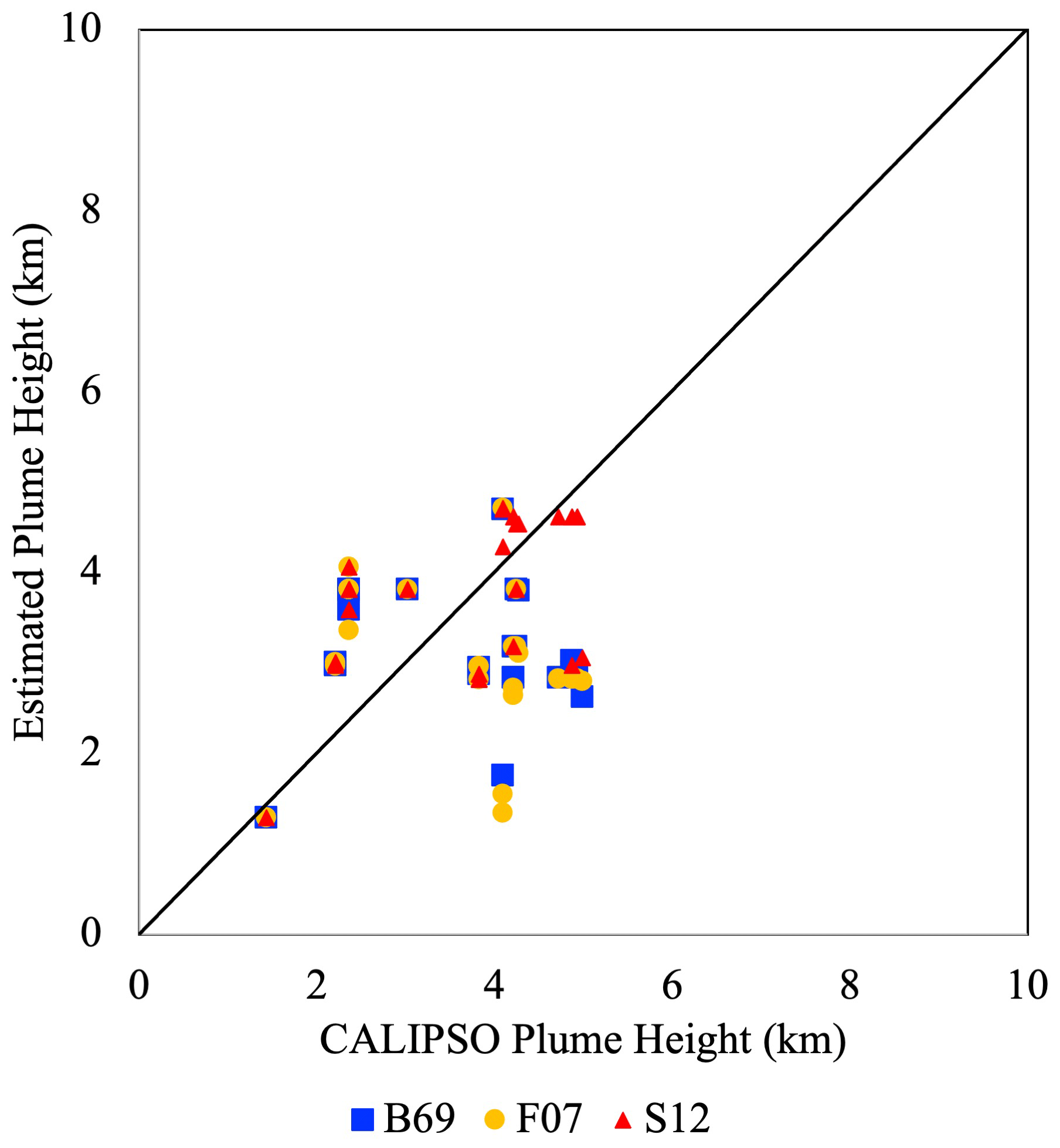
Figure 4Comparisons of plume-top heights from three simulations, namely B69 (blue rectangle), F07 (orange dot), and S12 (red triangle), against aerosol height observations from the CALIPSO for West Coast fires.
3.2 Impact of estimated plume rise on PM2.5 vertical distribution
In this section, we investigate the impact of plume injection height on different PM2.5 chemical components. Figure 5 shows the vertical profile of the 2-month average PM2.5 concentration for the three experiments. Over 2 months, B69 simulated a higher average plume height and injected more PM2.5 in the free troposphere than F07 and S12. Meanwhile, F07 simulated a lower average plume height and therefore kept more PM2.5 in the boundary layer than B69 and S12.
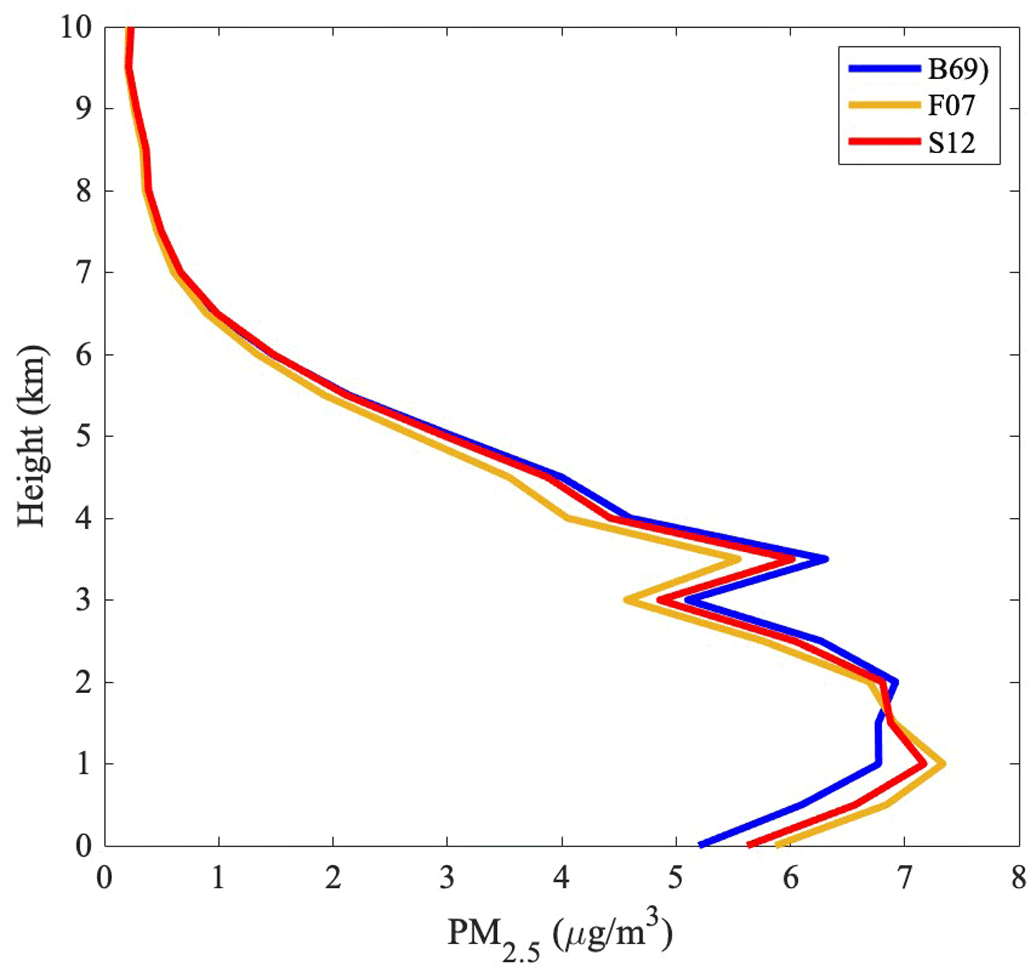
Figure 5Vertical profile of 2-month average PM2.5 concentration for B69, F07, and S12 in the CONUS domain.
Figure 6 shows the distribution of simulated PM2.5 components from both direct emissions and secondary formation (the impact of other PM2.5 sources was removed by subtracting the results of NoFire run) from B69, F07, and S12 in three different regions, namely western USA (west of 120∘ W), central USA (between 120 and 100∘ W), and eastern USA (between 100 and 80∘ W). For all three schemes, organic matter (OM) dominates the chemical composition of PM2.5, with 63 %–64 % near the source region in western USA, and remains dominant in the downwind regions at ∼61 %, between 120 and 100∘ W, and 57 %, between 100 and 80∘ W. A high-OM portion highlights the predominant effect of wildfire emissions on air quality during the gigafire period (Li et al., 2021). The second most abundant component is nitrate (NO3), with 11 %–12 % near the source region and 13 %–16 % in the downwind region. A higher portion of NO3 in the downwind region than in the source region reflects the decreased contribution of primary aerosols and increases in secondary aerosols. The other component with a similar spatial gradient is ammonium (NH4), which contributes 3 % to PM2.5 near the source region and 5 %–6 % in the downwind region. Elemental carbon contributes 10 % to PM2.5 concentration near the source region and 8 %–9 % in the downwind region. Potassium (K), a fingerprint element to indicate fire contribution, accounts for 3 % of PM2.5 near the source region and 2 %–3 % in the downwind region. Sulfate (SO4) contributed 3 % near the source region and 6 %–8 % in the downwind region. In summary, PM2.5 species that are not significantly affected by secondary aerosol formation, such as elemental carbon and potassium, see a decrease in their contributions when transported downwind. For the PM2.5 species that are affected by secondary aerosol formation (e.g., nitrate, sulfate, and ammonium), the contribution increases when transported downwind. These results show that the PM2.5 composition, integrated over all vertical layers, is not sensitive to the choice of plume rise scheme.
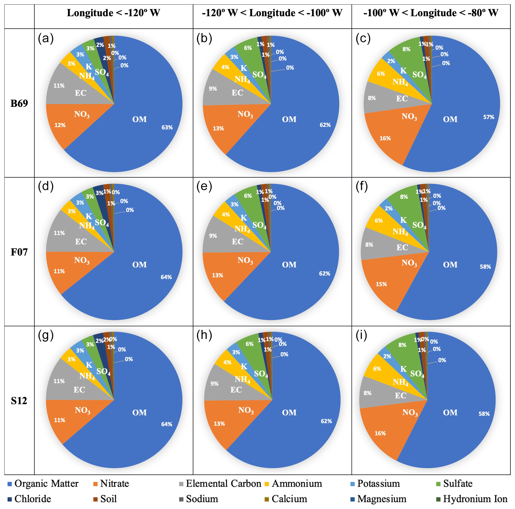
Figure 6The simulated PM2.5 chemical components (%) with the B69, F07, and S12 plume rise schemes in three different regions, i.e., to the west of 120∘ W (a, d, g), between 120 and 100∘ W (b, e, h), and between 100 and 80∘ W (c, f, i). The data are integrated over all vertical layers and averaged during the analysis period. The top six components are labeled in each plot.
Figure 7 shows the difference in the zonal mean (average for each latitude) concentrations of six major PM2.5 species (i.e., organic matter, nitrate, elemental carbon, ammonium, potassium, and sulfate) and total PM2.5 when using different plume rise schemes over the whole domain. Overall, most of the differences are found over the West Coast region (to the west of 115∘ W). The simulation with B69 produces a higher plume height on average, resulting in greater transport of smoke aloft, and hence higher downwind PM2.5 than that with the F07 or S12 schemes. The B69 plume rise scheme has a higher downwind impact and slightly lower near-source impact for PM2.5 species that contain secondary aerosols (e.g., organic matter, nitrate, ammonium, and sulfate) than primary aerosols (e.g., elemental carbon and potassium), due to the time required to form secondary aerosols.
Among the three simulations, the largest differences in PM2.5 are found from the surface to 8 km over the source region. Over the downwind region, the bulk of PM2.5 differences is found in the middle and upper troposphere. In addition, we noticed that the simulations with F07 and S12 produce more PM2.5 than that with B69 between 6–8 km during the analysis period. This is because, in the cases of a strong fire, the plume injection height simulated by F07 or S12 could be higher than B69 (e.g., Fig. 3e). However, the difference in PM2.5 above 6 km is very small compared to those particles below 6 km. The total PM2.5 difference caused by different plume rise schemes is about 30 % near the source and 5 % in the downwind region. The difference in surface PM2.5 has a large impact on surface pollution levels and human health. More discussion on the impact of plume height on surface air quality is presented in Sect. 3.4. Although the upper-level PM2.5 difference is expected to have a smaller impact on human health, it may affect cloud formation, photochemical reactions, and the radiative budget in the Earth system.
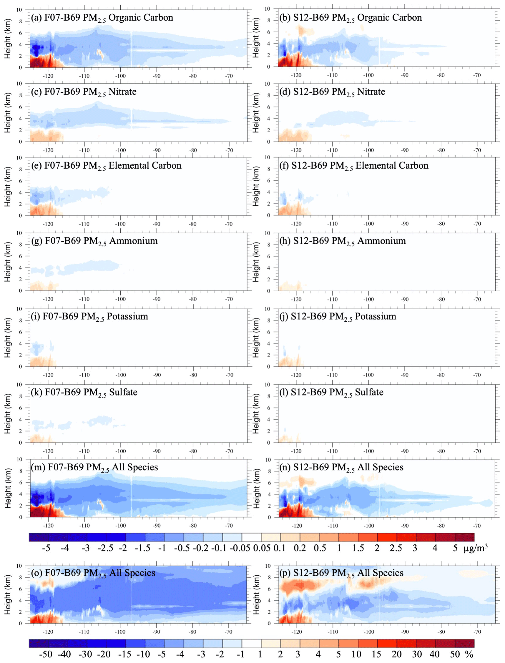
Figure 7(a–n) Zonal mean difference in predicted concentrations of six major PM2.5 species among the simulations using the B69, F07, and S12 schemes from 1 August to 30 September 2020 for organic matter (a, b), nitrate (c, d), elemental carbon (e, f), ammonium (g, h), potassium (i, j), and sulfate (k, l). The difference in total PM2.5 is displayed by both the absolute values (m, n) and percentage (o, p).
3.3 Impact of estimated plume rise on aerosol optical depth and photochemistry
Wildfire smoke increases the aerosol loading in the atmosphere and consequently the AOD over both the source region and downwind regions. According to our previous study (Li et al., 2021), from 14–17 September 2020 smoke from the West Coast was transported to the northeastern part of the USA. The downwind transport of wildfire smoke is highly dependent on plume rise estimation. Figure 8a shows the 2-month-averaged AOD from VIIRS compared with model simulations (Fig. 7b–d). The CMAQ-predicted AOD was interpolated to the VIIRS pixels that passed quality control using the nearest-neighbor approach. When comparing the CMAQ AOD to VIIRS AOD (Fig. 7b–d), we applied VIIRS AOD saturation level (AOD ≤5) to CMAQ AOD results (any CMAQ AOD values higher than 5 were changed to 5). In the West Coast high-peak region, all three runs capture the observed AOD high peak near the San Francisco region, but the simulated AOD peak is lower than VIIRS observed. The average AOD from VIIRS observation is higher than 2. However, among the three CMAQ runs, only F07 simulated an average AOD higher than 2. In the downwind region, all three CMAQ runs reproduce the general downwind transport pattern, but the simulated smoke-affected region (AOD >0.5) is smaller than the observations.
Figure 7e–h show the AOD differences and the difference ratio (percentage of the difference relative to B69) between the different plume rise scheme simulations. When comparing different model simulations, the AOD saturation level is removed. Near the source region, F07 and S12 simulate more AOD than B69, a pattern that is the opposite of that for plume rise estimation (lower plume height than that with B69). In the downwind region, B69 simulates more AOD than F07 and S12. The difference is approximately 20 %–30 % over the source region and 5 %–10 % over the downwind region. One possible reason that B69 predicts lower AOD near the source region and higher AOD in the downwind region compared to F07 and S12 is that a higher plume height will inject more aerosol into the free troposphere where the wind speed is stronger, accelerating the dispersion of the fire pollution. Therefore, the higher plume height will lead to lower AOD near the source region but higher AOD in the downwind region. The result is consistent with previous studies (Mallia et al., 2018; Vernon et al., 2018; Li et al., 2020).
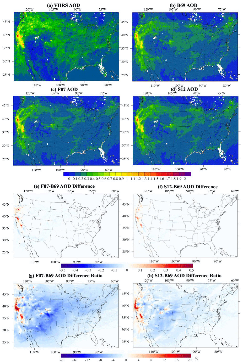
Figure 8The 2-month average AOD from VIIRS (a), B69 run (b), F07 run (c), and S12 run (d) from 1 August to 30 September 2020. The average AOD differences between F07 and B69 (e) and between S12 and B69 (f) during the same period as in panel (a). The average AOD difference ratio between F07 and B69 (g) and between S12 and B69 (h) during the same period as in panel (a).
The difference in the dispersion of fire pollution caused by the various estimated plume injection heights leads to further differences in the chemistry and photolysis reactions. Previous studies found that the thicker smoke, indicated by higher AOD, may absorb and/or scatter a larger fraction of sunlight, hence affecting photolysis reactions (Dickerson et al., 1997; Castro et al., 2001; Kumar et al., 2014; Baylon et al., 2018). Here, we simply examine how the plume rise differences affects photochemistry by comparing the photolysis rate of NO2 (NO NO + O) from the three runs, which is a key reaction that leads to the formation of tropospheric ozone. The differences in the NO2 photolysis rate (NO2_IUPAC10; in min−1) are shown in Fig. 9. Figure 9a and d show the photolysis rate difference and difference ratio between B69 and the NoFire experiments. The photolysis rate results in B69 were lower than the NoFire simulation, which proves that fire smoke led to the reduction in the photolysis rate, consistent with the findings of previous studies. The photolysis rate reduction caused by the fire smoke was found in the whole domain, both in the near-source region and the downwind region. Near the fire source, the photolysis rate reduction was more than 50 %. Figure 9b, c, e, and f show the photolysis rate difference and difference ratio between the three experiments with different plume rise schemes. Near the source region, where F07 and S12 simulate a higher AOD than B69 (Fig. 8), the NO2_IUPAC10 is reduced. Meanwhile, in the downwind region, where F07 and S12 simulate a lower AOD, the photolysis rate is higher than B69. Therefore, the difference in the plume injection height would affect the fire-induced photolysis rate reduction.
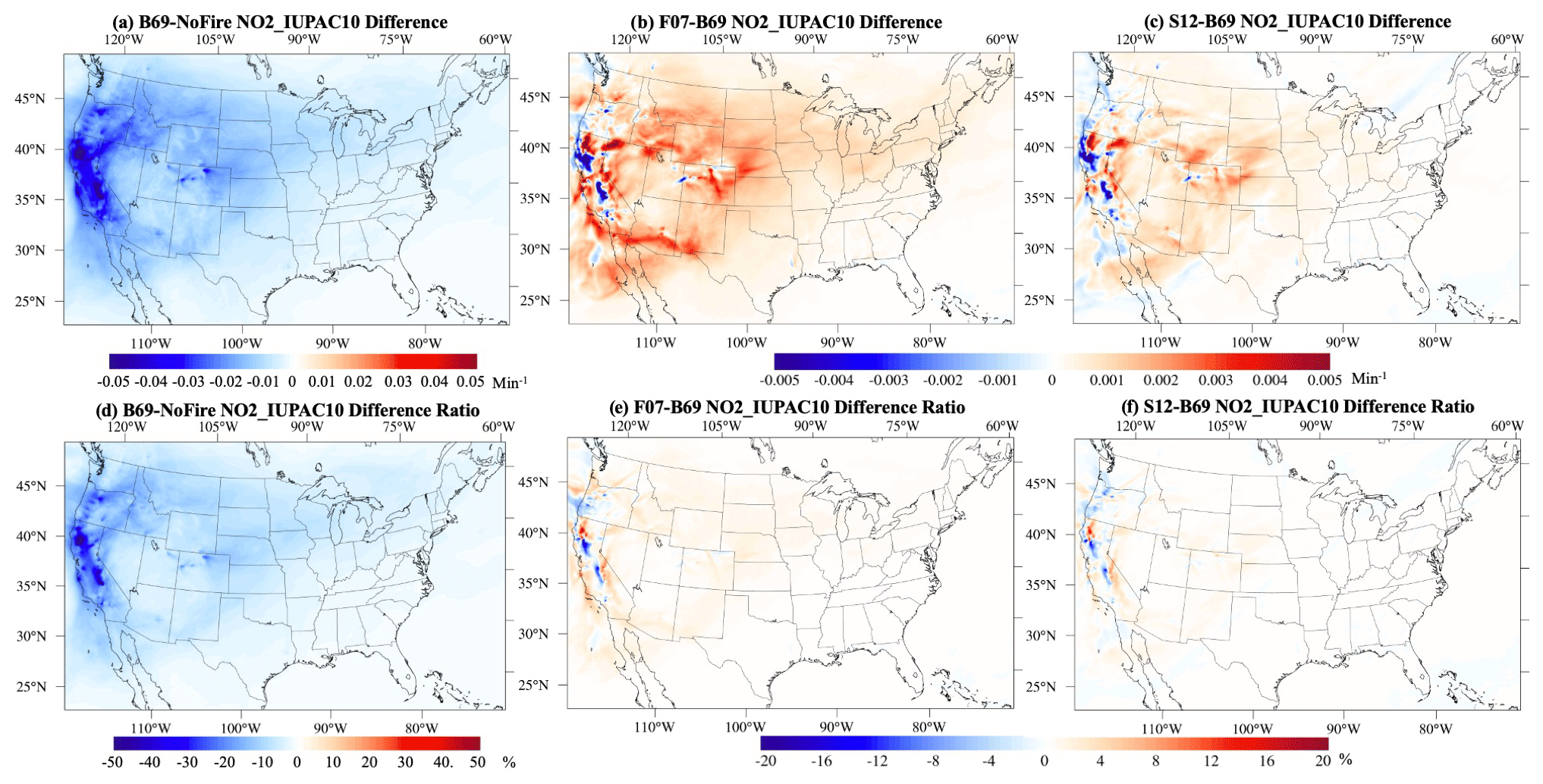
Figure 9The average photolysis rate NO2_IUPAC10 differences between B69 and NoFire (a), between F07 and B69 (b), and between S12 and B69 (c) from 1 August to 30 September 2020. The average photolysis rate NO2_IUPAC10 difference ratio between B69 and NoFire (d), between F07 and B69 (e), and between S12 and B69 (f) during the same period.
3.4 Impact of estimated plume rise on surface PM2.5 and exceedance of NAAQS
Surface or ambient PM2.5 is the common measure used to link exposure to wildfire smoke to health endpoints such as asthma and chronic obstructive pulmonary disease (Reid et al., 2016). To protect human health and the environment, the National Ambient Air Quality Standards (NAAQS) have been established for PM2.5 and other criteria air pollutants (NO2, O3, SO2, CO, PM10, and lead). The daily PM2.5 NAAQS level is 35 µg m−3 for the 24 h mean PM2.5 concentration (United States Environmental Protection Agency, 2020b). The simulated surface PM2.5 differences caused by different plume rise schemes are shown in Fig. 10. The F07 and S12 simulations, which have averaged lower initial plume heights, yield higher surface PM2.5 concentrations than the B69 simulation over the West Coast, whereas the opposite patterns are found in the central and the eastern USA. The surface PM2.5 difference caused by different plume rise schemes reaches 70 % over the West Coast, which is much higher than the AOD differences. In the downwind regions, the surface PM2.5 difference caused by different plume rise schemes is less than 15 %, meaning that the effects of the plume rise estimation on surface PM2.5 occur mainly near the source region.
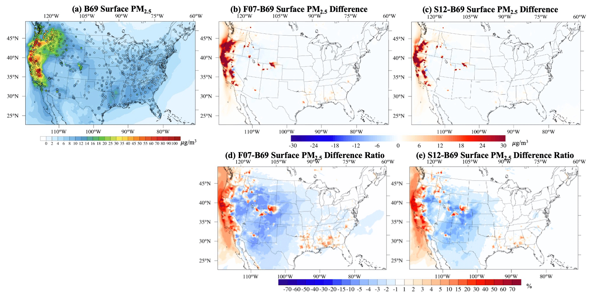
Figure 10Simulated and observed surface PM2.5 from 1 August to 30 September 2020. (a) Average surface PM2.5 simulated with B69 overlaid by AirNow observations. (b) Difference in averaged surface PM2.5 between F07 and B69. (c) Difference between S12 and B69. Panels (d) and (e) are the same as panels (b) and (c) but for the differences in percentage (%) between F07 and B69 and between S12 and B69, respectively.
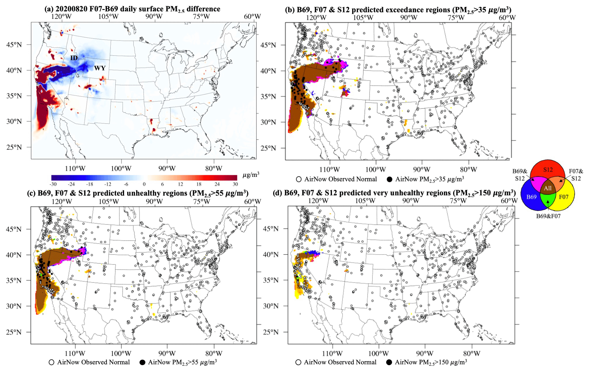
Figure 11Predicted surface PM2.5 concentrations above unhealthy levels by the S12, F07, and B69 runs for 20 August 2020. (a) The daily mean surface PM2.5 difference between F07 and B69 runs. (b) Simulated PM2.5 exceedance regions by B69, F07, and S12 overlaid by AirNow observed exceedance (PM2.5>35 µg m−3). Panel (c) is the same as panel (b) but for U.S. EPA-defined unhealthy regions (PM2.5>55 µg m−3). Panel (d) is the same as panel (b) but for U.S. EPA-defined very unhealthy regions (PM2.5>150 µg m−3). The brown color represents the region where the runs with all three schemes simulate PM2.5 exceedances. The blue (red/yellow) color represents the region where only B69 (S12 or F07) simulates the PM2.5 exceedance. The green color represents the region where both the B69 and F07 simulate the PM2.5 exceedance. The magenta color represents the region where both the B69 and S12 simulate the PM2.5 exceedance. The orange color represents the region where both F07 and S12 simulate the PM2.5 exceedance.
Next, we examine how the plume rise estimation affects the prediction of PM2.5 exceedances. Figure 11a shows the daily mean surface PM2.5 difference between the F07 and B69 runs for 20 August 2020 (the first fire peak during the study period). The simulated PM2.5 exceedance regions (PM2.5>35 µg m−3, as defined by NAAQS, and at same level as U.S. EPA-defined unhealthy regions for sensitive groups), unhealthy regions (PM2.5>55 µg m−3, as defined by U.S. EPA), and very unhealthy regions (PM2.5>150 µg m−3, as defined by U.S. EPA) as seen by different plume rise schemes overlaid by the AirNow-observed exceedance for the same day are shown in Fig. 10b, c, and d. According to Fig. 11b and c, on 20 August 2020, B69 and S12 simulated more PM2.5 exceedance and a larger unhealthy region in the downwind regions (Wyoming (WY) and Idaho (ID); magenta and blue region), whereas F07 and S12 simulated more exceedance and a larger unhealthy region in the southeastern USA (yellow and orange region), where prescribed fires were the major biomass burning sources. In WY and ID, where F07 did not simulate the PM2.5 exceedance, whereas B69 and S12 did, the difference between F07 and B69 reached 15 µg m−3 (Fig. 11a). Furthermore, B69 and S12 simulate some very unhealthy regions in Nevada, whereas F07 simulates more very unhealthy regions in central and southern California. Although these schemes agree on the PM2.5 exceedance forecast in the majority of the region, the disagreements in the downwind areas (i.e., ID and WY for this case) may affect key decision-making on early warnings of extreme air pollution episodes at local levels during large wildfire events.
The total number of predicted exceedance days from the B69 simulation and the differences between B69, F07, and S12 are shown in Fig. 12. All the states on the West Coast and in the mountain region experienced at least 1 d of PM2.5 exceedance (Fig. 12a). Most of the region in northern California experienced more than 20 exceedance days, with a maximum of more than 35 d. F07 and S12 simulate more exceedance days on the West Coast near the source region and in the southeast. The difference in the exceedance days could be as large as 20 d in northern California. B69 simulates more exceedance days in downwind regions such as Nevada, Idaho, Montana, and Wyoming. The difference could reach 4 d in the downwind regions.
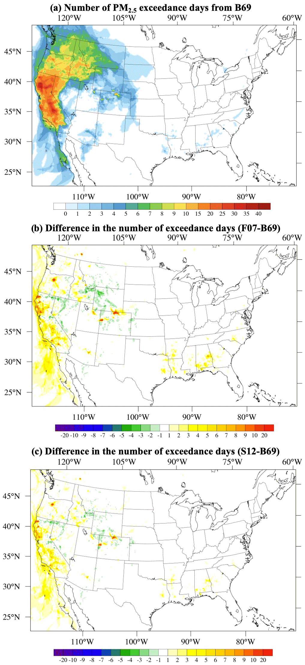
Figure 12The CMAQ B69-predicted total number of PM2.5 exceedance days during August–September 2020 (a). The difference in the number of predicted exceedance days between B69 and F07 (b) and between B69 and S12 (c).
In this study, we use CMAQ with three different plume rise schemes, namely Briggs (1969; B69), Freitas et al. (2007; F07), and Sofiev et al. (2012; S12), to understand the impact of plume rise calculation on aerosol and photochemistry during the 2020 western USA wildfire season. The plume heights simulated by all three schemes are comparable to MISR and CALIPSO observations of aerosol height. The performance of the simulations with different schemes varies for different fire cases and weather conditions (i.e., humidity). On average, the B69 predicts higher injection heights than F07 and S12, leading to higher downwind PM2.5 concentrations due to the stronger transport at the higher altitude. The largest PM2.5 differences are found from the surface to 8 km over the source region. Over the downwind region, the bulk of the PM2.5 differences is found in the middle and upper troposphere. The total PM2.5 difference is approximately 30 % near the source and 5 % in the downwind region. Furthermore, we found that the plume rise scheme has a higher downwind impact and slightly lower near-source impact for PM2.5 species that contain more secondary aerosols than primary aerosols.
Thick fire smoke also increases AOD in the source and the downwind regions. On average, F07 and S12, which estimate lower plume height, simulate greater smoke AOD near the fire source region than B69. In the downwind region, B69 simulates higher AOD than F07 and S12. The difference is approximately 20 %–30 % near the source region and 5 %–10 % in the downwind region. When AOD is higher, the thicker smoke may block more sunlight and affect the photolysis reaction rates. Near the source region, where F07 and S12 simulate a higher AOD, the photolysis reaction rate decreases.
Finally, we analyzed the effect of plume rise estimation on the prediction of PM2.5 exceedances. The F07 and S12 simulations, which have lower averaged plume heights, predict higher surface PM2.5 concentrations than B69 over the West Coast, whereas the opposite patterns are found in the central and the eastern USA. The effects of the plume rise estimation on surface PM2.5 occur mainly near the source region. The surface PM2.5 difference caused by different plume rise schemes reaches 70 % over the West Coast and is less than 15 % in the downwind regions. These results suggest that the effects of plume rise estimation on surface PM2.5 occur mainly near the source region, whereas in the downwind region, the majority of effects are in the free troposphere. For the PM2.5 exceedance prediction, higher plume height produces a larger PM2.5 exceedance area in the downwind region. In most affected areas, the predicted PM2.5 exceedance regions from the three schemes overlapped. In non-overlapping regions, the simulated differences in PM2.5 could reach 15 µg m−3. For the whole period of study, the difference in the total number of exceedance days could be as large as 20 d in northern California and 4 d in the downwind regions. F07 and S12 simulated more exceedance days near the fire source region, while B69 simulates more exceedance days in downwind regions such as Nevada, Idaho, Montana, and Wyoming. Such PM2.5 exceedance forecast differences may affect key decision-making on early warnings of extreme air pollution episodes at local levels during large wildfire events.
The WRF-CMAQ system used in this study is an offline model. The heat emitted by the fire calculated in the CMAQ does not influence the meteorology model (WRF), such as the PBL height, temperature, and wind field. In the future, online models will be utilized to further study the plume rise estimation impacts on air quality.
CMAQ documentation and released versions of the source code are available on the U.S. EPA modeling site https://doi.org/10.5281/zenodo.3585898 (United States Environmental Protection Agency, 2020a). The WRF V4.2 model code is distributed by National Center for Atmospheric Research: https://github.com/wrf-model/WRF (National Center for Atmospheric Research, 2020).
The MISR, GBBEPx, VIIRS, and AirNow data used in this paper can be found at https://doi.org/10.5281/zenodo.7702951 (Li et al., 2023).
YL and DT designed the study and performed the research, with contributions from all co-authors. SRF, RA, MS, and GG prepared the plume rise code. SM, XZ, SK, and FL prepared fire emission data. RK prepared the MISR data and guided the evaluation of plume height estimation. YL and DT wrote and revised the paper, with input from YT, BB, and PC. All authors commented on drafts of the paper.
The contact author has declared that none of the authors has any competing interests.
Publisher's note: Copernicus Publications remains neutral with regard to jurisdictional claims in published maps and institutional affiliations.
This article is part of the special issue “The role of fire in the Earth system: understanding interactions with the land, atmosphere, and society (ESD/ACP/BG/GMD/NHESS inter-journal SI)”. It is a result of the EGU General Assembly 2020, 4–8 May 2020.
This work has been financially supported by the NASA Health and Air Quality Program, NOAA Weather Program Office, and George Mason University College of Science. The observation data from NASA, NOAA, and U.S. EPA are gratefully acknowledged.
This research has been supported by the Earth Sciences Division (NASA Health and Air Quality Program) and the NOAA Research, NOAA Weather Program Office (NOAA Weather Program Office).
This paper was edited by Yuan Wang and reviewed by three anonymous referees.
Ahmadov, R., Grell, G., James, E., Csiszar, I., Tsidulko, M., Pierce, B., McKeen, S., Benjamin, G., Alexander, C., Pereira, G., Freitas, S., and Goldberg, M.: Using VIIRS Fire Radiative Power data to simulate biomass burning emissions, plume rise and smoke transport in a real-time air quality modeling system, Ieee International Geoscience and Remote Sensing Symposium, IEEE International Symposium on Geoscience and Remote Sensing IGARSS, New York, Ieee, 2806-8, 2017.
Akagi, S. K., Yokelson, R. J., Burling, I. R., Meinardi, S., Simpson, I., Blake, D. R., McMeeking, G. R., Sullivan, A., Lee, T., Kreidenweis, S., Urbanski, S., Reardon, J., Griffith, D. W. T., Johnson, T. J., and Weise, D. R.: Measurements of reactive trace gases and variable O3 formation rates in some South Carolina biomass burning plumes, Atmos. Chem. Phys., 13, 1141–1165, https://doi.org/10.5194/acp-13-1141-2013, 2013.
Amiridis, V., Giannakaki, E., Balis, D. S., Gerasopoulos, E., Pytharoulis, I., Zanis, P., Kazadzis, S., Melas, D., and Zerefos, C.: Smoke injection heights from agricultural burning in Eastern Europe as seen by CALIPSO, Atmos. Chem. Phys., 10, 11567–11576, https://doi.org/10.5194/acp-10-11567-2010, 2010.
Archer-Nicholls, S., Lowe, D., Darbyshire, E., Morgan, W. T., Bela, M. M., Pereira, G., Trembath, J., Kaiser, J. W., Longo, K. M., Freitas, S. R., Coe, H., and McFiggans, G.: Characterising Brazilian biomass burning emissions using WRF-Chem with MOSAIC sectional aerosol, Geosci. Model Dev., 8, 549–577, https://doi.org/10.5194/gmd-8-549-2015, 2015.
Baek, B. H. and Seppanen, C.: CEMPD/SMOKE: SMOKE v4.7 Public Release (October 2019), Zenodo [code], https://doi.org/10.5281/zenodo.3476744, 2019.
Baylon, P., Jaffe, D. A., Hall, S. R., Ullmann, K., Alvarado, M. J., and Lefer, B. L.: Impact of biomass burning plumes on photolysis rates and ozone formation at the Mount Bachelor Observatory, J. Geophys. Res.-Atmos., 123, 2272–2284, https://doi.org/10.1002/2017JD027341, 2018.
Briggs, G. A.: Plume rise, Tech. Rep. Crit. Rev. Ser., 81 pp., Natl. Tech. Inf. Serv., Springfield, VA, 1969.
Briggs, G. A.: Some recent analyses of plume rise observations, Proceedings of the Second International Clean Air Congress, edited by: Englund, H. M. and Beery, W. T., Academic Press, New York, 1029–1032, 1971.
Briggs, G. A.: Discussion on chimney plumes in neutral and stable surroundings. Atmos. Environ., 6, 507–510, 1972.
Byun, D. W. and Schere, K. L.: Review of the governing equations, computational algorithms, and other components of the models-3 community multiscale air quality (CMAQ) modeling system, Appl. Mech. Rev., 59, 51–77, https://doi.org/10.1115/1.2128636, 2006.
Cascio, W. E.: Wildland fire smoke and human health, Sci. Total Environ., 624, 586–595, https://doi.org/10.1016/j.scitotenv.2017.12.086, 2018.
Castro, T., Madronich, S., Rivale, S., Muhlia, A., and Mar, B.: The influence of aerosols on photochemical smog in Mexico City, Atmos. Environ., 35, 1765–1722, 2001.
Dickerson, R. R., Kondragunta, S., stenchikov, G., Civerolo, K. L., Doddridge, B. G., and Holben, B. N.: The impact of aerosols on solar ultraviolet radiation and photochemical smog, Science, 278, 827–830, https://doi.org/10.1126/science.278.5339.827, 1997.
Diner, D. J., Beckert, J. C., Reilly, T. H., Bruegge, C. J., Conel, J. E., Kahn, R. A., Martonchik, J. V., Ackerman, T. P., Davies, R., Gerstl, S. A. W., Gordon, H. R., Muller, J.-P., Myneni, R. B., Sellers, P. J., Pinty, B., and Verstraete, M. M.: Multi-angle Imaging SpectroRadiometer (MISR) instrument description and experiment overview, IEEE T. Geosci. Remote, 36, 1072–1087, 1998.
Draxler, R. R. and Hess, G. D.: An Overview of the HYSPLIT4 Modeling System of Trajectories, Dispersion, and Deposition, Australian Meteorological Magazine, 47, 295–308, 1998.
Eyth, A., Vukovich, J., and Farkas, C.: Technical Support Document (TSD) Preparation of Emissions Inventories for 2016v1 North American Emissions Modeling Platform, https://www.epa.gov/sites/default/files/2021-03/documents/preparation_of_emissions_inventories_for_2016v1_north_american_emissions_modeling_platform_tsd.pdf (last access: 1 March 2023), 2021.
Fahey, K. M., Carlton, A. G., Pye, H. O. T., Baek, J., Hutzell, W. T., Stanier, C. O., Baker, K. R., Appel, K. W., Jaoui, M., and Offenberg, J. H.: A framework for expanding aqueous chemistry in the Community Multiscale Air Quality (CMAQ) model version 5.1, Geosci. Model Dev., 10, 1587–1605, https://doi.org/10.5194/gmd-10-1587-2017, 2017.
Freeborn, P. H., Wooster, M. J., Hao, W. M., Ryan, C. A., Nordgren, B. L., Baker, S. P., and Ichoku, C.: Relationships between energy release, fuel mass loss, and trace gas and aerosol emissions during laboratory biomass fires, J. Geophys. Res., 113, D01301, https://doi.org/10.1029/2007JD008679, 2008.
Freitas, S. R., Longo, K. M., Chatfield, R., Latham, D., Silva Dias, M. A. F., Andreae, M. O., Prins, E., Santos, J. C., Gielow, R., and Carvalho Jr., J. A.: Including the sub-grid scale plume rise of vegetation fires in low resolution atmospheric transport models, Atmos. Chem. Phys., 7, 3385–3398, https://doi.org/10.5194/acp-7-3385-2007, 2007.
Grell, G. A. and Freitas, S. R.: A scale and aerosol aware stochastic convective parameterization for weather and air quality modeling, Atmos. Chem. Phys., 14, 5233–5250, https://doi.org/10.5194/acp-14-5233-2014, 2014.
Iacono, M. J., Delamere, J. S., Mlawer, E. J., Shephard, M. W., Clough, S. A., and Collins, W. D.: Radiative forcing by long-lived greenhouse gases: Calculations with the AER radiative transfer models, J. Geophys. Res., 113, D13103, https://doi.org/10.1029/2008JD009944, 2008.
Janjić, Z. I.: The Step-Mountain Eta Coordinate Model: Further developments of the convection, viscous sublayer, and turbulence closure schemes, Mon. Weather Rev., 122, 927–945, https://doi.org/10.1175/1520-0493(1994)122<0927:TSMECM>2.0.CO;2, 1994.
Johnston, F., Henderson, S., Chen, Y., Randerson, J., Marlier, M., DeFries, R., Kinney, P., Bowman, D., and Brauer M.: Estimated Global Mortality Attributable to Smoke from Landscape Fires, Environ Health Perspect., 120, 695–701, https://doi.org/10.1289/ehp.1104422, 2012.
Kahn, R. A., Chen, Y., Nelson, D. L., Leung, F.-Y., Li, Q., Diner, D. J., and Logan, J. A.: Wildfire smoke injection heights: Two perspectives from space, Geophys. Res. Lett., 35, L04809, https://doi.org/10.1029/2007GL032165, 2008.
Koning, H. W., Smith, K. R., and Last, J. M.: Biomass fuel combustion and health, Bulletin of the World Health Organization, 63, 11–26, 1985.
Koppmann, R., von Czapiewski, K., and Reid, J. S.: A review of biomass burning emissions, part I: gaseous emissions of carbon monoxide, methane, volatile organic compounds, and nitrogen containing compounds, Atmos. Chem. Phys. Discuss., 5, 10455–10516, https://doi.org/10.5194/acpd-5-10455-2005, 2005.
Koren, V., Schaake, J., Mitchell, K., Duan, Q.-Y., Chen, F., and Baker, J. M.: A parameterization of snowpack and frozen ground intended for NCEP weather and climate models, J. Geophys. Res., 104, 19569–19585, https://doi.org/10.1029/1999JD900232, 1999.
Kumar, R., Barth, M. C., Madronich, S., Naja, M., Carmichael, G. R., Pfister, G. G., Knote, C., Brasseur, G. P., Ojha, N., and Sarangi, T.: Effects of dust aerosols on tropospheric chemistry during a typical pre-monsoon season dust storm in northern India, Atmos. Chem. Phys., 14, 6813–6834, https://doi.org/10.5194/acp-14-6813-2014, 2014.
Laszlo, I. and Liu, H.: EPS Aerosol Optical Depth (AOD) Algorithm Theoretical Basis Document, https://www.star.nesdis.noaa.gov/jpss/documents/ATBD/ATBD_EPS_Aerosol_AOD_v3.4.pdf (last access: 1 March 2023), 2022.
Li, Y.: GMU-CMAQ PM2.5 forecast for 2020 GigaFire, Zenodo [data set], https://doi.org/10.5281/zenodo.7659096, 2023.
Li, Y., Tong, D. Q., Ngan, F., Cohen, M. D., Stein, A. F., Kondragunta, S., Zhang, X., Ichoku, C., Hyer, E., and Kahn, R.: Ensemble PM2.5 forecasting during the 2018 Camp Fire event using the HYSPLIT transport and dispersion model, J. Geophys. Res.-Atmos., 125, e2020JD032768, https://doi.org/10.1029/2020JD032768, 2020.
Li, Y., Tong, D., Ma, S., Zhang, X., Kondragunta, S., Li, F., and Saylor, R.: Dominance of wildfires impact on air quality exceedances during the 2020 record-breaking wildfire season in the United States, Geophys. Res. Lett., 48, e2021GL094908, https://doi.org/10.1029/2021GL094908, 2021.
Li, Y., Tong, D., Zhang, X., Kondragunta, S., and Kahn, R.: Fire emission, plume, and air quality observation for the 2020 US Giga Fire, Zenodo [data set], https://doi.org/10.5281/zenodo.7702951, 2023.
Liu, Y., Austin, E., Xiang, J., Gould, T., Larson, T., and Seto, E.: Health impact assessment of the 2020 Washington State wildfire smoke episode: Excess health burden attributable to increased PM2.5 exposures and potential exposure reductions, GeoHealth, 5, e2020GH000359, https://doi.org/10.1029/2020GH000359, 2021.
Luecken, D. J., Yarwood, G., and Hutzell, W. H.: Multipollutant of ozone, reactive nitrogen and HAPs across the continental US with CMAQ-CB6, Atmos. Environ., 201, 62–72, https://doi.org/10.1016/j.atmosenv.2018.11.060, 2019.
Mallia, D., Kochanski, A., Urbanski, S., and Lin, J.: Optimizing Smoke and Plume Rise Modeling Approaches at Local Scales, Atmosphere, 9, 166, https://doi.org/10.3390/atmos9050166, 2018.
Mazzoni, D., Logan, J. A., Diner, D., Kahn, R. A., Tong, L., and Li, Q.: A data-mining approach to associating MISR smoke plume heights with MODIS fire measurements, Remote Sens. Environ., 107, 138–148, 2007.
Morrison, H., Thompson, G., and Tatarskii, V.: Impact of cloud microphysics on the development of trailing Stratiform precipitation in a simulated squall line: Comparison of one- and two-moment schemes, Mon. Weather Rev., 137, 991–1007, https://doi.org/10.1175/2008MWR2556.1, 2009.
National Center for Atmospheric Research (NCAR): Weather Research and Forecasting Model, National Center for Atmospheric Research [code], https://github.com/wrf-model/WRF, last access: 1 February 2021.
National Interagency Fire Center: 2020 National Large Incident Year-to-Date Report (PDF), Geographic Area Coordination Center (Report), 21 December 2020.
Nelson, D. L., Garay, M. J., Kahn, R. A., and Dunst, B. A.: Stereoscopic Height and Wind Retrievals for Aerosol Plumes with the MISR INteractive eXplorer (MINX), Remote Sens., 5, 4593–4628, https://doi.org/10.3390/rs5094593, 2013.
O'Neill, S. M., Diao, M., Raffuse, S., Al-Hamdan, M., Barik, M., Jia, Y., Reid, S., Zou, Y., Tong, D., West, J., Wilkins, J., Marsha, A., Freedman, F., Vargo, J., Larkin, N., Alvarado, E., and Loesche, P.: A multi-analysis approach for estimating regional health impacts from the 2017 Northern California wildfires, J. Air Waste Manag. Assoc., 71, 791–814, https://doi.org/10.1080/10962247.2021.1891994, 2021.
Pal, S. R., Steinbrecht, W., and Carswell, A. I.: Automated method for lidar determination of cloud base height and vertical extent, Appl. Optics, 31, 1488–1494, 1992.
Pye, H. O. T., Luecken, D. J., Xu, L., Boyd, C. M., Ng, N. L., Baker, K. R., Ayres, B. R., Bash, J. O., Baumann, K., Carter, W. P. L., Edgerton, E., Fry, J. L., Hutzell, W. T., Schwede, D. B., and Shepson, P. B.: Modeling the current and future roles of particulate organic nitrates in the southerneastern United States, Environ. Sci. Technol., 49, 14195–14203, https://doi.org/10.1021/acs.est.5b03738, 2015.
Reid, C. E., Brauer, M., Johnston, F. H., Jerrett, M., Balmes, J. R., and Elliott, C. T.: Critical review of health impacts of wildfire smoke exposure, Environ. Health Perspect., 124, 1334–1343, 2016.
Roy, A., Choi, Y., Souri, A., Jeon, W., Diao, L., Pan, S., and Westenbarger, D.: Effects of Biomass Burning Emissions on Air Quality Over the Continental USA: A Three-Year Comprehensive Evaluation Accounting for Sensitivities Due to Boundary Conditions and Plume Rise Height, in: Environmental Contaminants. Energy, Environment, and Sustainability, edited by: Gupta, T., Agarwal, A., Agarwal, R., and Labhsetwar, N., Springer, Singapore, https://doi.org/10.1007/978-981-10-7332-8_12, 2017.
Schlosser, J. S., Braun, R. A., Bradley, T., Dadashazar, H., MacDonald, A. B., Aldhaif, A. A., Aghdam, M. A., Mardi, A. H., Xian, P., and Sorooshian, A.: Analysis of aerosol composition data for western United States wildfires between 2005 and 2015: Dust emissions, chloride depletion, and most enhanced aerosol constituents, J. Geophys. Res.-Atmos., 122, 8951–8966, https://doi.org/10.1002/2017JD026547, 2017.
Seinfeld, J. H. and Pandis, S. N.: Atmospheric Chemistry and Physics: From Air Pollution to Climate Change, 3rd edn., John Wiley & Sons, Hoboken, ISBN-10 1118947401; ISBN-13 978-1118947401, 2016.
Sessions, W. R., Fuelberg, H. E., Kahn, R. A., and Winker, D. M.: An investigation of methods for injecting emissions from boreal wildfires using WRF-Chem during ARCTAS, Atmos. Chem. Phys., 11, 5719–5744, https://doi.org/10.5194/acp-11-5719-2011, 2011.
Skamarock, W. C., Klemp, J. B., Dudhia, J., Gill, D. O., Liu, Z., Berner, J., Wang, W., Powers, J. G., Duda, M. G., Barker, D. M., and Huang, X.-Y.: A Description of the Advanced Research WRF Version 4, NCAR Tech. Note NCAR/TN-556+STR, 145 pp., https://doi.org/10.5065/1dfh-6p97, 2019.
Sofiev, M., Ermakova, T., and Vankevich, R.: Evaluation of the smoke-injection height from wild-land fires using remote-sensing data, Atmos. Chem. Phys., 12, 1995–2006, https://doi.org/10.5194/acp-12-1995-2012, 2012.
Tang, Y., Carmichael, G. R., Uno, I., Woo, J.-H., Kurata, G., Lefer, B., Shetter, R. E., Huang, H., Anderson, B. E., Avery, M. A., Clarke, A. D., and Blake, D. R.: Impacts of aerosols and clouds on photolysis frequencies and photochemistry during TRACE-P, part II: three-dimensional study using a regional chemical transport model, J. Geophys. Res., 108, 8822, https://doi.org/10.1029/2002JD003100, 2003.
Thapa, L. H., Ye, X., Hair, J. W., Fenn, M. A., Shingler, T., Kondragunta, S., Ichoku, C., Dominguez, R., Ellison, L., Soja, A. J., Gargulinski, E., Ahmadov, R., James, E., Grell, G. A., Freitas, S. R., Pereira, G., and Saide, P. E.: Heat flux assumptions contribute to overestimation of wildfire smoke injection into the free troposphere, Commun. Earth Environ., 3, 236, https://doi.org/10.1038/s43247-022-00563-x, 2022.
United States Environmental Protection Agency: CMAQ (Version 5.3.1), Zenodo [software], https://doi.org/10.5281/zenodo.3585898, (last access: 1 February 2021), 2020a.
United States Environmental Protection Agency: Review of the National Ambient Air Quality Standards for Particulate Matter, Federal Register, 85, December 18, 2020, 82684–82748, https://www.govinfo.gov/content/pkg/FR-2020-12-18/pdf/2020-27125.pdf (last access: 1 February 2021), 2020b.
Val Martin, M. V., Honrath, R. E., Owen, R. C., Pfister, G., Fialho, P., and Barata, F.: Significant enhancements of nitrogen oxides, black carbon, and ozone in the North Atlantic lower free troposphere resulting from North American boreal wildfires, J. Geophys. Res.-Atmos., 111, D23S60, https://doi.org/10.1029/2006JD007530, 2006.
Val Martin, M., Logan, J. A., Kahn, R. A., Leung, F.-Y., Nelson, D. L., and Diner, D. J.: Smoke injection heights from fires in North America: analysis of 5 years of satellite observations, Atmos. Chem. Phys., 10, 1491–1510, https://doi.org/10.5194/acp-10-1491-2010, 2010.
Val Martin, M., Kahn, R. A., Logan, J. A., Paugam, R., Wooster, M., and Ichoku, C.: Space-based observational constraints for 1-D fire smoke plume-rise models, J. Geophys. Res., 117, D22204, https://doi.org/10.1029/2012JD018370, 2012.
Val Martin, M., Kahn, R. A., and Tosca, M. G.: A Global Analysis of Wildfire Smoke Injection Heights Derived from Space-Based Multi-Angle Imaging, Remote Sensing, 10, 1609, https://doi.org/10.3390/rs1010, 2018.
Vernon, C. J., Bolt, R., Canty, T., and Kahn, R. A.: The impact of MISR-derived injection height initialization on wildfire and volcanic plume dispersion in the HYSPLIT model, Atmos. Meas. Tech., 11, 6289–6307, https://doi.org/10.5194/amt-11-6289-2018, 2018.
Wilmot, T. Y., Mallia, D. V., Hallar, A. G., and Lin, J. C.: Wildfire plumes in the Western US are reaching greater heights and injecting more aerosols aloft as wildfire activity intensifies, Sci. Rep., 12, 12400, https://doi.org/10.1038/s41598-022-16607-3, 2022.
Winker, D. M., Hunt, W. H., and McGill, M. J.: Initial performance assessment of CALIOP, Geophys. Res. Lett., 34, L19803, https://doi.org/10.1029/2007GL030135, 2007.
Wooster, M. J., Roberts, G., Perry, G. L. W., and Kaufman, Y. J.: Retrieval of biomass combustion rates and totals from fire radiative power observations: FRP derivation and calibration relationships between biomass consumption and fire radiative energy release, J. Geophys. Res., 110, D24311, https://doi.org/10.1029/2005JD006318, 2005.
Xu, L., Pye, H. O. T., He, J., Chen, Y., Murphy, B. N., and Ng, N. L.: Experimental and model estimates of the contributions from biogenic monoterpenes and sesquiterpenes to secondary organic aerosol in the southeastern United States, Atmos. Chem. Phys., 18, 12613–12637, https://doi.org/10.5194/acp-18-12613-2018, 2018.
Ye, X., Arab, P., Ahmadov, R., James, E., Grell, G. A., Pierce, B., Kumar, A., Makar, P., Chen, J., Davignon, D., Carmichael, G. R., Ferrada, G., McQueen, J., Huang, J., Kumar, R., Emmons, L., Herron-Thorpe, F. L., Parrington, M., Engelen, R., Peuch, V.-H., da Silva, A., Soja, A., Gargulinski, E., Wiggins, E., Hair, J. W., Fenn, M., Shingler, T., Kondragunta, S., Lyapustin, A., Wang, Y., Holben, B., Giles, D. M., and Saide, P. E.: Evaluation and intercomparison of wildfire smoke forecasts from multiple modeling systems for the 2019 Williams Flats fire, Atmos. Chem. Phys., 21, 14427–14469, https://doi.org/10.5194/acp-21-14427-2021, 2021.
Zhang, H., Kondragunta, S., Laszlo, I., Liu, H., Remer, L. A., Huang, J., Superczynski, S., and Ciren, P.: An enhanced VIIRS aerosol optical thickness (AOT) retrieval algorithm over land using a global surface reflectance ratio database, J. Geophys. Res.-Atmos., 121, 10717–10738, https://doi.org/10.1002/2016JD024859, 2016.
Zhang, X., Kondragunta, S., Ram, J., Schmidt, C., and Huang, H.-C.: Near-real-time global biomass burning emissions product from geostationary satellite constellation, J. Geophys. Res.-Atmos., 117, https://doi.org/10.1029/2012JD017459, 2012.
Zhang, X., Kondragunta, S., Da Silva, A., Lu, S., Ding, H., Li, F., and Zhu, Y.: The blended global biomass burning emissions product from MODIS and VIIRS observations (GBBEPx) version 3.1, https://www.ospo.noaa.gov/Products/land/gbbepx/docs/GBBEPx_ATBD.pdf (last access: 1 February 2021), 2019.