Variable effects of spatial resolution on modeling of nitrogen oxides

The lifetime and concentration of nitrogen oxides (NO_x) are susceptible to nonlinear production and loss and to the resolution of a chemical transport model (CTM). This is due to the strong spatial gradients of NO_x and the dependence of its own chemical loss on such gradients. In this study, we use the GEOS-Chem CTM in its high-performance implementation (GCHP) to investigate NO_x simulations over the eastern United States across a wide range of spatial model resolutions (six different horizontal grids from 13 to 181 km). Following increasing grid size, afternoon surface NO_x mixing ratios over July 2015 generally decrease over the Great Lakes region (GL) and increase over the southern states of the US region (SS), yielding regional differences (181 km vs. 13 km) of −16 % (in the GL) to 7 % (in the SS); meanwhile, hydrogen oxide radicals (HO_x) increase over both regions, consistent with their different chemical regimes (i.e., NO_x-saturated in the GL and NO_x-limited in the SS). Nighttime titration of ozone by surface nitric oxide (NO) was found to be more efficient at coarser resolutions, leading to longer NO_x lifetimes and higher surface mixing ratios of nitrogen dioxide (NO₂) over the GL in January 2015. The tropospheric NO₂ column density at typical afternoon satellite overpass time has spatially more coherent negative biases (e.g., −8 % over the GL) at coarser resolutions in July, which reversed the positive biases of surface NO_x over the SS. The reduced NO_x aloft (>1 km altitude) at coarser resolutions was attributable to the enhanced HO_x that intrudes into the upper troposphere. Application of coarse-resolution simulations for interpreting satellite NO₂ columns will generally underestimate surface NO₂ over the GL and overestimate surface NO₂ over the SS in summer, but it will uniformly overestimate NO_x emissions over both regions. This study significantly broadens understanding of factors contributing to NO_x resolution effects and the role of fine-resolution data in accurately simulating and interpreting NO_x and its relevance to air quality.

1 Introduction

Nitrogen oxides (NO_x≡ NO + NO₂) have major roles in tropospheric chemistry and air quality. During daytime, NO_x interacts with hydrogen oxide radicals (HO_x≡ OH + HO₂) and volatile organic compounds (VOCs) via photochemical reactions to affect formation of ozone and nitrate aerosols (e.g., Sillman, 1999; Thornton et al., 2002; Pusede et al., 2015; Zhu et al., 2022). During nighttime, persistent NO_x emissions are the main chemical sink of ozone in urban areas (Zhang et al., 2004; Brown et al., 2006; Zakoura and Pandis, 2018); meanwhile, sequential formation of the nitrate radical (NO₃) significantly alters nocturnal atmospheric oxidation capacity and secondary aerosols (Evans and Jacob, 2005; Brown and Stutz, 2012; Rollins et al., 2012). NO_x has strongly localized emissions (Miyazaki et al., 2017; Crippa et al., 2018; Beirle et al., 2019) and relatively short lifetimes (Kenagy et al., 2018; Laughner and Cohen, 2019), which determine its strong spatial heterogeneity, with a short e-folding distance of 30 km and less (Heue et al., 2008; Beirle et al., 2011; Valin et al., 2011). While such localization is advantageous for identifying and quantifying NO_x emissions using observations such as satellite nitrogen dioxide (NO₂) column density (e.g., Martin et al., 2006; Cooper et al., 2017; Goldberg et al., 2019; Laughner and Cohen, 2019; Wang et al., 2022), it poses a challenge for chemical transport models (CTMs) attempting to accurately represent the relevant production and loss processes at interurban scales (on the order of 10 km) due to limited computational resources.

One major issue is the resolution dependence of simulated NO_x lifetime (τ) (Charlton-Perez et al., 2009; Valin et al., 2011), which is sensitive to NO_x abundance itself due to the interaction of NO_x with its own chemical loss (Laughner and Cohen, 2019; Shah et al., 2020), such as hydroxyl radical (OH) and ozone (e.g., Fig. A1a). Systematic differences in the simulated τ and NO_x concentration at different resolutions were reported from simulated NO_x plumes of power plants, cities and ship emissions (Sillman et al., 1990; Charlton-Perez et al., 2009; Valin et al., 2011) due to the stronger NO_x localization at higher resolution. Regional chemical transport modeling with more realistically distributed emissions was also performed to examine how NO_x abundance changes with varying resolutions (Valin et al., 2011; Yamaji et al., 2014; Yan et al., 2016; Yu et al., 2016). The majority of these studies indicated increased τ and NO_x concentration at higher resolutions and attributed it to the titration of OH by NO_x over sources in the NO_x-saturated regime (e.g., the right part of Fig. A1a). However, evidence (Laughner and Cohen, 2019; Jin et al., 2020; Zhu et al., 2022) has emerged that many cities across the United States (US) recently experienced the transition into the NO_x-limited regime following emission regulations, where stronger NO_x emissions actually promote HO_x production and decrease τ (e.g., the left part of Fig. A1a). It is unclear how this change will update our understanding of the spatial resolution dependency of simulated NO_x. Furthermore, nighttime effects have rarely been studied, possibly due to the prolonged τ localization and reduced NO_x localization, although the significant spatial heterogeneity of nocturnal NO_x and ozone in urban environments has still been noted (Zhang et al., 2004; Pan et al., 2017; Zakoura and Pandis, 2018), and long-term effects of changing NO_x on nighttime τ have also been found (Shah et al., 2020). Finally, retrieval of tropospheric NO₂ column density (Ω) from a growing constellation of satellite instruments (e.g., OMI, TROPOMI, TEMPO, Sentinel-4, GEMS) offers observational information to constrain NO_x emissions across vast continental and global regions (Veefkind et al., 2012; Streets et al., 2013; Zoogman et al., 2017; Levelt et al., 2018; Timmermans et al., 2019; Kim et al., 2020). Existing studies have not separately discussed the resolution effects on Ω and surface NO_x, which can potentially differ due to the vertically nonuniform spatial heterogeneity and species abundances.

Given that numerous existing studies depicted an evident yet potentially incomplete mechanistic understanding, this study uses a CTM across a wide range of spatial resolutions to significantly enrich the current understanding of the resolution dependency of NO_x simulations. We find evidence over the eastern US that changes in simulated NO_x abundances at different resolutions are by no means uniform but instead depend on factors such as chemical regimes, dominant processes and vertical layering. This information urges future studies to apply an adequate resolution that captures the spatial scale of NO_x sources and sinks to simulate and interpret NO_x-relevant atmospheric chemistry and air quality issues.

2 Materials and methods

We use the GEOS-Chem model in its high-performance implementation (GCHP, http://www.geos-chem.org, last access: February 2022, version 13.2.1, https://doi.org/10.5281/zenodo.5500718; The International GEOS-Chem User Community, 2021) to simulate NO_x and its relevant components over the eastern US.

GCHP is a grid-independent implementation of GEOS-Chem operating in a distributed-memory framework for massive parallelization (Long et al., 2015; Eastham et al., 2018). Chemical transport is simulated using a finite-volume advection code (FV3) on a cubed-sphere grid (Putman and Lin, 2007). GCHP uses identical chemistry and physics modules as the traditional GEOS-Chem implementation (GEOS-Chem Classic). A stretched-grid capability offers finer resolution over a user-specified domain of interest (Bindle et al., 2021). The model version used here (v13.2.1) features significant advances for performance and ease of use (Martin et al., 2022). The model is driven by the Goddard Earth Observation System Forward Processing (GEOS-FP) assimilated meteorological data, with a native resolution of 0.25^∘ × 0.3125^∘, from the NASA Global Modeling and Assimilation Office (GMAO). The GEOS-FP data are currently the finest-resolution meteorology available for GCHP simulations for the simulation year and were regridded to each simulation resolution, including a resolution (of 13 km) that is finer than 0.25^∘ × 0.3125^∘. Although nonideal, this capability, as demonstrated by Bindle et al. (2021), will not significantly alter our interpretations, which focus on discussing the redistribution of NO_x emissions and chemical feedbacks rather than effects from meteorology. Yan et al. (2016) showed that sub-coarse-grid emission–chemical variability dominantly contributed to the differences in simulated tropospheric chemistry between resolutions, overwhelming the effects from resolution of nonchemical factors such as meteorological data. Consistent with GEOS-FP, the atmosphere is vertically distributed into 72 layers (from surface to 0.01 hPa) following the hybrid sigma-pressure grid definition during the simulation. Boundary layer mixing is simulated with a nonlocal scheme (Lin and McElroy, 2010). The lowest layer is roughly 120 m thick, with mixing ratios of NO_x, HO_x and ozone that we refer to as the “surface concentrations” or “surface mixing ratios” interchangeably.

We use the standard full-chemistry scheme of the GEOS-Chem model, which is widely used to study air quality (Koplitz et al., 2016; Li et al., 2017; Shah et al., 2020; Gu et al., 2021). The scheme includes detailed gas-phase mechanisms of HO_x–NO_x–VOC–ozone chemistry (Bey et al., 2001; Mao et al., 2013; Sherwen et al., 2016), including heterogeneous uptake of reactive gases (McDuffie et al., 2018; Holmes et al., 2019) by the simultaneously simulated aerosols. Anthropogenic NO_x emissions are from EDGAR v5.0 at 0.1^∘ resolution (Crippa et al., 2021), and speciated anthropogenic non-methane VOC emissions are from CEDS v2 (Hoesly et al., 2018). Open-burning emissions are from GFED v4.1 (van der Werf et al., 2017). Although the latter two inventories have nonideal (0.5^∘ and 0.25^∘) resolutions due to availability, they are acceptable for the purpose of identifying the resolution dependence of NO_x. One favorable capability of the simulation is the pre-calculated offline dust, lightning NO_x, biogenic VOCs (BVOCs), soil NO_x and sea salt aerosol emissions (Murray et al., 2012; Weng et al., 2020; Meng et al., 2021), which all avoid possible regional emission biases due to online calculations using meteorological fields at different resolutions and the consequent interference with the interpretation of the results. All of the emissions are handled by the HEMCO 3.0 module (Keller et al., 2014; Lin et al., 2021).

We conduct GCHP simulations for January (winter) and July (summer) of 2015 at six resolutions spanning the range of conventional global model capabilities (Table 1). The highest resolution (13 km) is close to the currently finest information from emission inventories (0.1^∘) in global CTMs without downscaling, and the lowest resolution (181 km) remains widely used in global and regional air quality studies (i.e., similar to 2^∘ × 2.5^∘ resolution). For the three relatively coarse resolutions, we conduct global cubed-sphere simulations, while for resolutions <50 km we exploited the recently developed grid-stretching capability (Bindle et al., 2021) to greatly reduce the computational resource requirements. The stretched-grid configuration smoothly decreases the grid cell size towards the refined region of interest. We follow recommendations by Bindle et al. (2021) to choose moderate stretch factors (Table 1), ensuring that the lowest resolutions (i.e., on the antipode of the refined region) remain finer than 300 km while achieving substantially refined resolutions over the eastern US (Table 1, right).

Table 1 Description of the simulations with six resolutions over the eastern US.

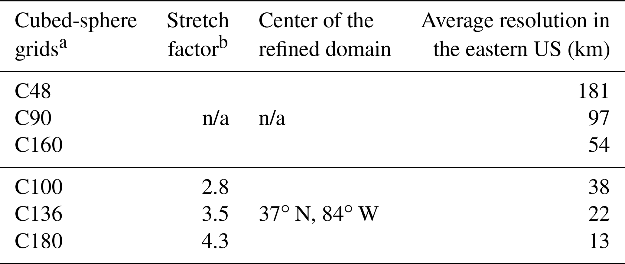
^a A cubed-sphere grid contains a mosaic of six grids (faces). Each face is regularly spaced with N×N grid cells, and the notation of each resolution (CN) here identifies the size N. ^b Stretch factor (S) defines the strength of the grid-stretching. The resolution is about S times higher than the regular cubed sphere over the refined region (eastern US), while it is about $\mathrm{1}/S$ of the original resolution over the antipode (n/a: not applicable).

In this work, we apply chemical operator durations of 20 min and transport operator durations of 10 min (i.e., C20T10) (Philip et al., 2016) to all of the simulations, largely in accordance with the GCHP default for cubed-sphere simulations, while avoiding interferences with our interpretation from inconsistent operator duration settings.

Initial conditions on 1 December 2014 and 1 June 2015 are obtained from a 1-year spin-up run of the C360 global cubed-sphere simulation using identical model version and inputs. These initial conditions resemble a realistic global high-resolution (∼ 25 km) distribution of NO_x-relevant species and their oxidants driven by the consistent emissions and chemistry used in this study and were then regridded to drive the 2-month simulations at each resolution. The second month (January and July 2015) from each simulation is used for the analysis to allow for a further spin-up at each resolution. We archive the hourly average model outputs to enable the detailed discussion in Sect. 3.

Figure 1a shows the study domain of interest (26–48^∘ N and 70–98^∘ W) and the emission ratio of isoprene to NO_x. The northern part of the domain comprises some of the most populous cities on the continent (e.g., New York City, Toronto and Chicago), with strong and localized NO_x emissions as observed from space (Russell et al., 2012; Lu et al., 2015; Laughner and Cohen, 2019), ideal for investigating NO_x resolution dependence. The southern regime is characteristic of the strongest biogenic VOC (e.g., isoprene) emission rates across the US (Romer et al., 2016; Yu et al., 2016; Jin et al., 2020) that could affect NO_x lifetime and its response to resolution.

Figure 1 Afternoon (UTC 19–24 or CST 13–18) resolution effects of surface NO_x mixing ratio driven by NO_x–HO_x feedbacks (e.g., Fig. A1a) over July 2015. (a) Emission ratio of isoprene vs. NO_x. (b) Simulated HO_x–NO_x relationship at each resolution (color coded). The contour lines (for resolutions <60 km) include 90 % of the scatter (points) of data within each 2^∘ × 2^∘ window centered over each city (based on kernel density estimation), and the circles indicated the means for all resolutions. (c) Surface NO_x mixing ratio at 13 km (top left) and the differences (minus 13 km) at the other resolutions (other subpanels). The regional mean NO_x (for 13 km, in ppbv) and percentage biases (for the other resolutions) are indicated at the bottom right of each subpanel. Green and magenta (rectangles, city names and numbers) label the Great Lakes region and the southern states of the US as defined in this study, respectively.

To assess the implications for interpreting satellite observations of NO₂, we also apply monthly mean scattering weights (w) (Palmer et al., 2001) from the TROPOspheric Monitoring Instrument (TROPOMI) at its overpass time (19:00–21:00 UTC, i.e., 13:00–15:00 CST, central standard time) to calculate NO₂ line-of-sight (slant) column density (Ω_s). Comparing Ω_s with Ω enables investigation of effects of satellite sensitivity on the resolution dependency of NO₂ columnar abundances. TROPOMI is currently the only instrument with sufficient fine resolution to provide w information for all the investigated resolutions over the study domain. We assign every clear-sky (i.e., geometric cloud fraction <0.2) TROPOMI w in January or July 2019 to the colocated grid cells of each resolution to derive the monthly mean w distribution, which is then applied to the afternoon mean NO₂ profiles in the same month of 2015 for each grid cell to calculate Ω_s. These mean scattering weights are dependent primarily on observing geometry and relative vertical profiles of molecular and aerosol scattering (Palmer et al., 2001; Cooper et al., 2020), which are expected to be similar in the same month among proximal years.

In this study, all of the regridding procedures between different resolutions are conducted using the conservative (surface-area-weighted) algorithm (https://earthsystemmodeling.org/regrid/, last access: February 2022) in the Earth System Modeling Framework.

3 Results

3.1 Daytime resolution effects at the surface in summer

Figure 1c shows the afternoon (19:00–24:00 UTC, corresponding to 13:00–18:00 CST) resolution effects of simulated surface NO_x mixing ratios over the eastern US in July 2015. At the finest resolution of 13 km (Fig. 1c, upper left), NO_x exhibits notable local enhancements over cities and major industrial corridors due to its short lifetime (τ, several hours). Overall, the stronger emissions and agglomerate sources in the Great Lakes region (GL, green box) lead to higher NO_x levels than in the southern states of the US region (SS, magenta box) where NO_x sources are relatively weak and sparse. As the grid cell size increases to 22 km resolution, the NO_x level shows an overall decrease over emission centers and increase over nearby grids (by up to 1 ppbv) relative to 13 km, an expected consequence due to dilution of emissions. However, systematic biases in predicted NO_x relative to 13 km resolution start to emerge, especially further downwind of urban NO_x sources and over the SS, reflecting the effects from the resolution-dependent τ. The biases relative to 13 km resolution become increasingly pronounced and regionally coherent as grid cells further enlarge. At the two lowest resolutions (>90 km), a clear dipole of negative biases over the GL and positive biases over the SS becomes visible.

The opposite resolution effects of simulated NO_x over the GL and SS are summarized as regional mean biases in each subpanel of Fig. 1c (e.g., −15.5 % at 181 km over the GL), which gradually increase in magnitude following increasing grid cell sizes, and these effects are attributable to their corresponding chemical regimes. The GL in summer is characterized by stronger NO_x emissions and lower VOC emissions, while the opposite scenario prevails over the SS with strong BVOC sources, partially characterized by the distribution of the isoprene$/$NO_x emission ratio in Fig. 1a. Consequently, the NO_x sources in the GL tend to be located in the NO_x-saturated regime (Fig. A1a, right), where concentrated NO_x levels at higher resolutions consume more OH and increase τ. Meanwhile, over the SS the relatively low NO_x, together with the enhanced VOCs, can in contrast promote HO_x production at higher NO_x levels (NO_x-limited regime, Fig. A1a, left), and thus the higher resolution introduces higher OH and lower τ. The lower τ can be a result of directly scavenging NO₂ via the enhanced OH and of indirectly reducing nitric oxide (NO) via the OH-promoted organic peroxy radicals (RO₂), an important NO_x sink pathway under low-NO_x and high-VOC environments (i.e., the SS) (Browne and Cohen, 2012; Perring et al., 2013; Romer et al., 2016; Romer Present et al., 2020). As NO_x emissions continue to decrease, multiple lines of evidence suggest that NO_x sources across the United States have recently entered or are approaching the NO_x-limited regime (Laughner and Cohen, 2019; Jin et al., 2020; Koplitz et al., 2021; Jung et al., 2022; Zhu et al., 2022), especially over the SS since the 2010s (Jin et al., 2020; Koplitz et al., 2021; Zhu et al., 2022).

Figure 1b shows examples of afternoon HO_x–NO_x relationships for 12 cities. We use HO_x to identify the regime representation since OH is unstable and has a very short lifetime (<1 s). HO_x and NO_x are anti-correlated over the GL (green label) and positively correlated over the SS (magenta label), consistently indicative of their different chemical regimes. Additionally, Figs. 1c and A2b show that (at 13 km resolution) locations with strong NO_x enhancements coincide with locally lower HO_x in the GL and generally associate with enhanced HO_x in the SS. The mean NO_x concentrations (circles) in Fig. 1b thus roughly decrease over the GL and increase over the SS following the opposite changes in τ as grid cell size increases (i.e., from purple to brown circles). The mean HO_x biases within the 2^∘ × 2^∘ windows above the cities are uniformly positive due to the opposite HO_x–NO_x associations over the GL and SS. Figure A2b further identifies the broadly uniformly positive simulation biases of HO_x in response to the opposite changes in NO_x in the two regions, consistently verifying the two chemical regimes.

The spatial extent of chemical regimes and their effects on the NO_x biases vary during the course of the day and contribute to relatively weak sensitivity of simulated NO_x to resolution in the SS. Figure A3 shows the resolution dependence of simulated surface NO_x for morning hours. Relative to the overall effects during afternoon (Fig. 1c), the NO_x-saturated regime (with negative NO_x biases at coarser resolution) has a broader extent (e.g., intruding further into the south) in the morning hours, whereas locations with positive biases (NO_x-limited regime) are substantially reduced. The magnitudes of NO_x bias (e.g., 181 km vs. 13 km) are also enhanced over the GL in the morning (−27.8 %). These differences are consistent with the relative diel evolution of NO_x (decreasing since sunrise) and HO_x (accumulating and peaking after noon) abundances and the consequence on the dominant HO_x loss pathway (e.g., Ren et al., 2003; Ma et al., 2022).

Another potential cause of the relatively weak sensitivity of simulated NO_x to resolution in the SS is the impact from BVOCs in addition to NO_x heterogeneity. Figure A1b shows that changing VOC reactivity mainly affects OH concentration and τ over the NO_x-limited regime but has little effect on the NO_x-saturated regime, consistent with previous studies (Edwards et al., 2014; Laughner and Cohen, 2019; Zhu et al., 2022). Apart from increasing OH, which decreases τ (Fig. A1b), decreasing VOCs can also decrease the strength of the NO–RO₂ loss pathway and increase τ (Browne and Cohen, 2012). Nonetheless, both processes indicate an increasing sensitivity of τ to VOCs in low-NO_x environments (Romer et al., 2016; Laughner and Cohen, 2019; Romer Present et al., 2020). The SS features strong BVOC emissions and strong spatial segregation of NO_x and VOC sources (Yu et al., 2016; Travis et al., 2016), as reflected by lower isoprene$/$NO_x emission ratios in urban centers relative to its neighborhood in Fig. 1a. Such segregation is reduced as the resolution coarsens (e.g., Fig. S1). The concurrent and usually opposite changes in NO_x (increases) and BVOC (decreases) emissions around NO_x sources at higher resolutions can jointly lead to the overall small changes among resolutions in the SS relative to in the GL. In summary, our simulations reveal that the predictability of actual resolution dependency of NO_x in the NO_x-limited regime is reduced due to the joint sensitivities to VOCs.

3.2 Nighttime resolution effects at surface in winter

Figure 2a shows the surface NO_x mixing ratio and its resolution dependence at nighttime (03:00–10:00 UTC or 21:00–04:00 CST) in January 2015. With prolonged τ (∼ 20 h) as photochemistry ceases and OH becomes negligible, the wintertime and nighttime NO_x exhibits reduced spatial heterogeneity (e.g., Fig. S2) relative to summertime and daytime in Fig. 1c, and thus the resolution effects are also less pronounced (i.e., ≤5 %). However, one characteristic phenomenon at nighttime that depends on resolution is the titration between NO and ozone (O₃), which are the main nighttime sinks to each other in urban environments (Brown et al., 2006; Wang et al., 2006; Brown and Stutz, 2012; Kenagy et al., 2018; Shah et al., 2020). Figure 2b and 2c indicate that the titration between NO and O₃ at the surface is enhanced by enlarged grid cells, as both concentrations were nearly uniformly reduced (by up to ∼ 50 % and ∼ 10 %, respectively) across the domain. At coarser resolutions, the faster O₃ titration produces more NO₂, complemented by less efficient scavenging of NO₂ by the more titrated O₃ (Fig. 2d). The resolution effect on surface NO_x (Fig. 2a) is thus jointly contributed by the opposite changes in NO (Fig. 2b) and NO₂ (Fig. 2d), the latter being more determinant due to its stronger contribution to total NO_x.

Figure 2 Nighttime (03:00–10:00 UTC or 21:00–04:00 CST) resolution effects of surface NO_x concentration driven by NO titration of O₃ (e.g., Fig. A4) during January 2015. Each panel is similar to Fig. 1c but for nighttime surface mixing ratios of (a) NO_x, (b) NO, (c) O₃ and (d) NO₂.

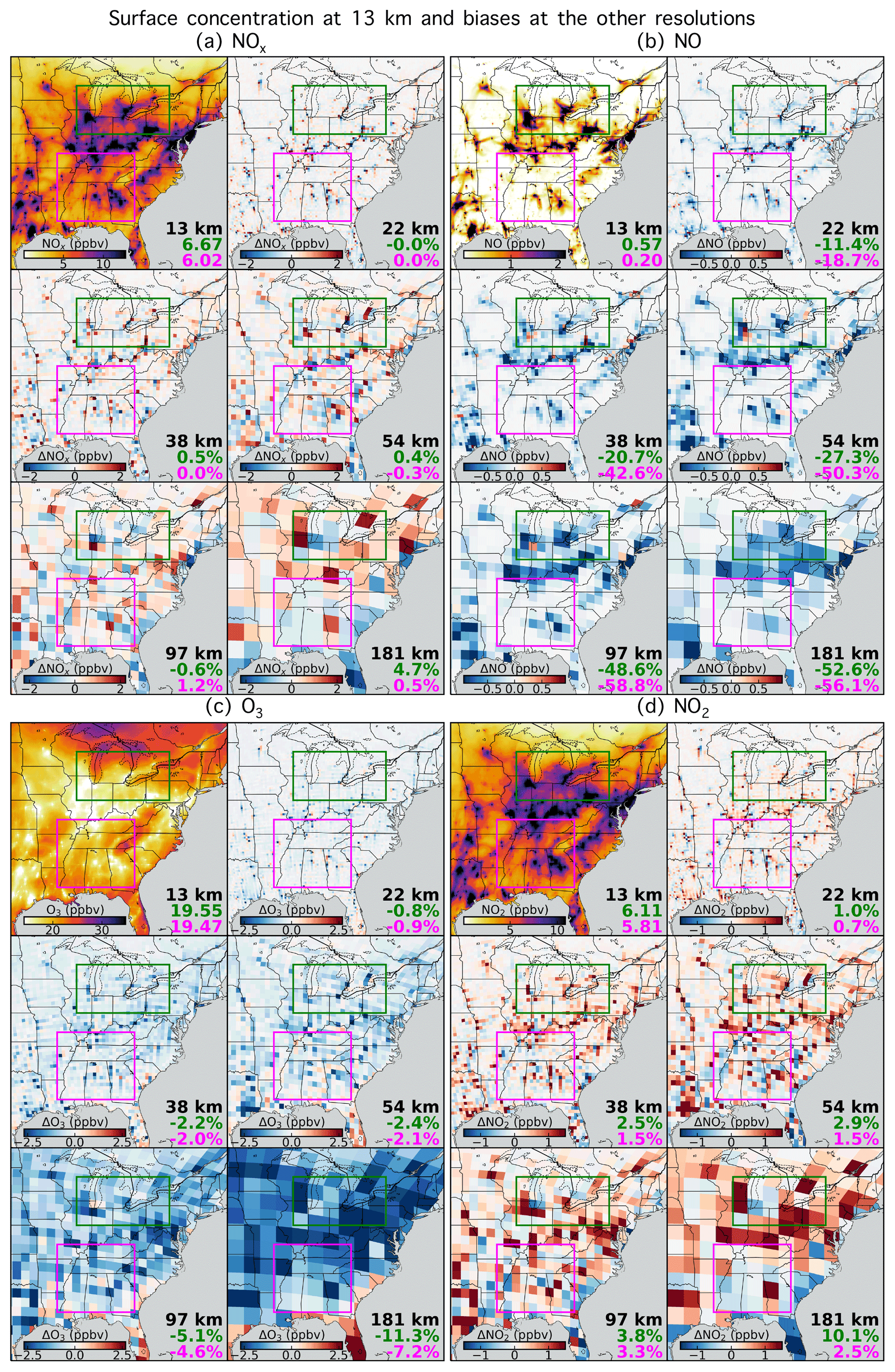
The faster titration efficiency at coarser resolution is driven by the spatial anti-correlation of NO and O₃, as demonstrated by Fig. A4. Typical nighttime high-NO regions are coincident with low-O₃ locations at 13 km resolution (first row), a result of daytime O₃ formation suppression and nighttime O₃ titration (Jacob et al., 1995; Zhang et al., 2004; Jin et al., 2017; Yan et al., 2018; Sicard et al., 2020; Li et al., 2022) over strong NO_x sources. This anti-correlation at fine resolution leads to inefficient NO–O₃ reaction, which is to first-order proportional to their products, shown in the third column of Fig. A4. By simply diluting their concentrations to larger grid cells (second–sixth rows), the products of NO–O₃ from less anti-correlated concentrations are enhanced systematically. Consequently, there would also be faster production of N₂O₅ and nitrates, which have been proposed by Zakoura and Pandis (2018) as an explanation for systematic overprediction of nitrate aerosols by CTMs at coarse resolution.

As the GL region has greater NO mixing ratios than the SS (Fig. 2b), surface O₃ is more effectively titrated (Fig. 2c), leading to increased NO₂ and NO_x concentrations (Fig. 2d). Meanwhile, over the SS the NO₂ response is less pronounced due to the lower NO levels, and NO₂ exhibits reductions over certain locations at lower resolutions (Fig. 2d), indicating that the excess O₃ can consume more NO₂ after titrating NO over these grids.

3.3 Seasonal and diel variation in relevant processes

Figure 3 summarizes the resolution effects of regional mean surface NO_x, HO_x and ozone at different hours of the day. Over the GL, the strongest percentage biases of regional mean NO_x (mainly NO₂, Fig. S3) at resolutions >13 km occur at nighttime in January (up to 5 %) and during daytime in July (up to −30 %), revealing a pronounced seasonality of dominant mechanisms driving the resolution effects. This seasonality is driven by the stronger intensity and duration of daytime oxidant production in July (i.e., purple lines for HO_x and O₃ in Fig. 3); meanwhile, the greater nighttime O₃ titration at coarser resolution partially counteracts the daytime effects in July (i.e., reduces the percentage biases) and dominates in January.

Figure 3 Resolution effects of surface NO_x dominated by nighttime biases in January and by daytime biases in July 2015. The absolute monthly mixing ratios (left y axis) of regional mean NO_x, HO_x and O₃ are shown as circles and solid lines at 13 km resolution, and the differences vs. 13 km resolution (right y axis) are shown as dashed lines for the other resolutions (see legend in the lower-right subpanel). The positive (light red) and negative (light blue) difference regimes are divided by color.

The SS region has relatively strong daytime resolution sensitivity that compensates for the opposite nighttime effects on NO₂ in January (Fig. S3), resulting in overall small changes in NO_x. In July, the resolution effects exhibit both the daytime photochemical processes and titration-driven nighttime effects, especially the unique positive biases of both NO_x and HO_x (NO_x-limited regime), during afternoon hours. Compared to the GL, July and daytime biases over the SS are not strong enough (e.g., discussions in Sect. 3.1) to mask the nighttime effects.

Overall, the daytime resolution effects driven by the involvement of NO_x in HO_x and O₃ production (Sect. 3.1) compete with the nighttime effects driven by NO_x-O₃ titration (Sect. 3.2). The changing dominance of each mechanism during summer vs. winter, as well as during daytime and nighttime, leads to the characteristic seasonal and diel variation in Fig. 3.

3.4 Vertically variable resolution effects

Figure 4 shows the resolution-dependent changes in regional mean afternoon NO_x vertical profiles in the lower troposphere (below 4 km). Uniform decreases in the simulated afternoon NO_x following larger grid cells are apparent at >1 km altitude in July, despite opposite changes over the two regions near the surface being present (Fig. 1). These vertically dependent responses are caused by the different vertical profiles of NO_x and HO_x (i.e., purple lines). As NO_x mixing ratio decreases exponentially aloft while HO_x increases (in the GL) or remains relatively uniform (in the SS), HO_x becomes more abundant relative to NO_x at higher altitudes, meaning that τ is less sensitive to NO_x local mixing ratios even above strong NO_x sources. The enhanced oxidants (ozone and HO_x) due to surface NO_x emission heterogeneity (Sect. 3.1) then vertically mix to systematically enhance the HO_x profile (Fig. 4, right) and reduce τ and NO_x in these aloft layers. Therefore, both regions exhibit negative NO_x biases due to coarse resolution above 1 km, regardless of chemical regime.

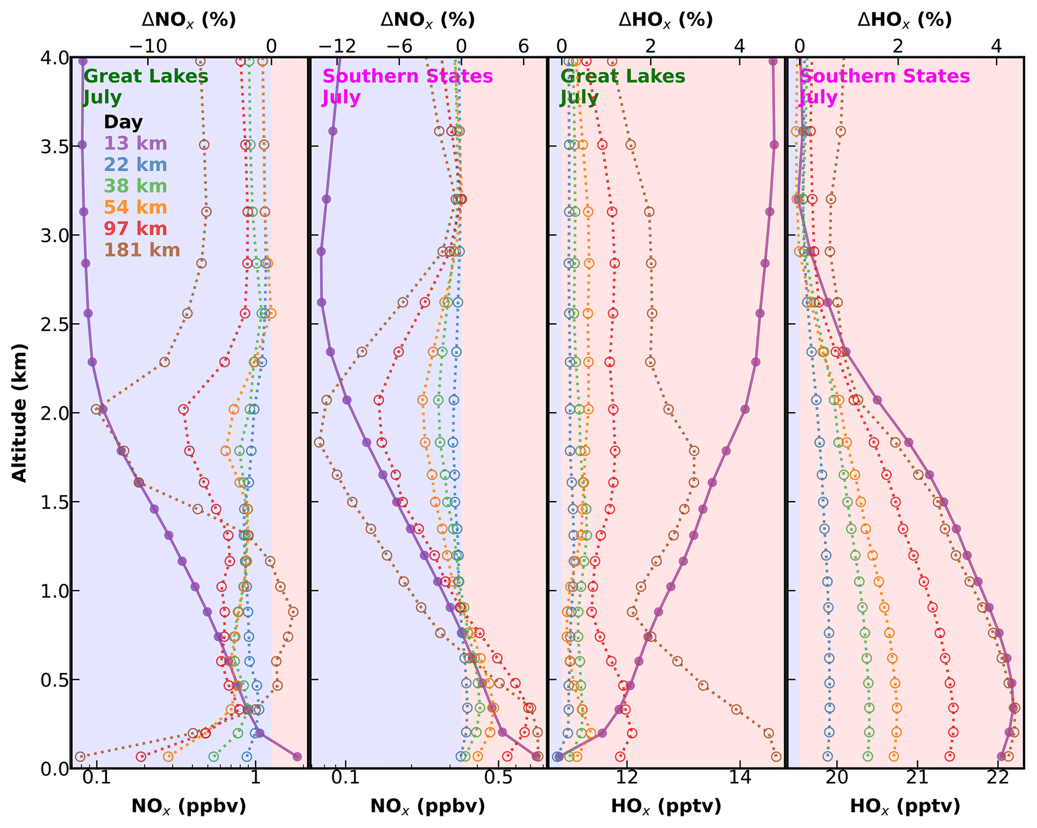
Figure 4 Change in afternoon NO_x vertical distribution in the lower troposphere at different resolutions in July. The absolute monthly and regional mean mixing ratios (lower x axis) of NO_x and HO_x are shown as filled symbols and solid lines at 13 km resolution, respectively, and the differences vs. 13 km resolution (upper x axis) are shown as empty symbols and dashed lines for the other resolutions, respectively (see legend in the left column). The positive (light red) and negative (light blue) difference regimes are color-divided.

Figure 5 shows the changes in the nighttime vertical profiles of NO_x and O₃ in January. These again show opposite vertical distributions of NO_x and its nighttime sink (ozone). Over the GL, although the surface NO_x lifetime can be possibly prolonged at coarse resolution due to the faster titration of O₃ by NO (Sect. 3.2), NO quickly becomes insufficient to titrate the increasing ozone at higher altitudes. Therefore, both NO_x species ultimately become affected by the resolution-dependent titration efficiency above 1 km (similar to the surface responses over the SS), leading to the negative biases in simulated NO_x regardless of surface NO_x emission strength.

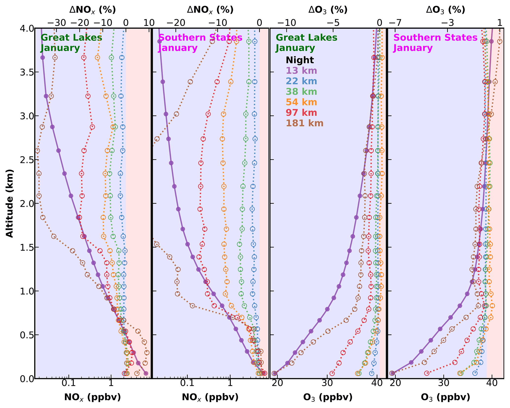
Figure 5 Change in nighttime NO_x vertical distribution in the lower troposphere at different resolutions in January. Similar to Fig. 4 but for nighttime NO_x and O₃ in January.

In summary, Figs. 4 and 5 reveal that the resolution effects of τ at the surface can differ from those at elevated altitudes, even over source regions. Such altitude-dependent responses will further affect interpretation of satellite-retrieved NO₂ columnar properties, using model simulations at these resolutions.

3.5 Implications for satellite remote sensing applications

Satellite retrievals of NO₂ vertical column density (Ω) have been widely used to quantify and characterize spatiotemporal variation in NO_x abundances and sources. Here we evaluate the implications of the NO_x resolution dependency on two major applications – estimating surface NO₂ concentration and deriving NO_x emissions.

Figure 6 shows the simulated fraction of NO₂ abundance within the surface layer of GEOS-Chem relative to the whole troposphere during low Earth orbit (LEO) afternoon satellite overpass time. This surface fraction (F_s) is lower in summer than in winter, driven by stronger convection, lightning NO_x and an elevated boundary layer. F_s is also lower over the SS than the GL in July due to relatively weak NO_x emissions at the surface and stronger lightning NO_x emissions in the upper troposphere (Murray et al., 2012; Silvern et al., 2019; Zhu et al., 2019). The changes in F_s following varying resolutions in general qualitatively resemble those of surface NO_x (e.g., when comparing Fig. 6 with Figs. 1c and 2a). Overall, F_s has stronger biases in July than in January, lowered by 10 % over the GL and enhanced by 4 % over the SS at 181 km, relative to 13 km resolution. As F_s is a key parameter in estimating surface NO₂ concentration from satellite-retrieved Ω (Lamsal et al., 2008; Cooper et al., 2020), directly applying the simulated NO₂ vertical profiles will propagate such resolution-dependent biases that also vary regionally and seasonally, as indicated in Fig. 6.

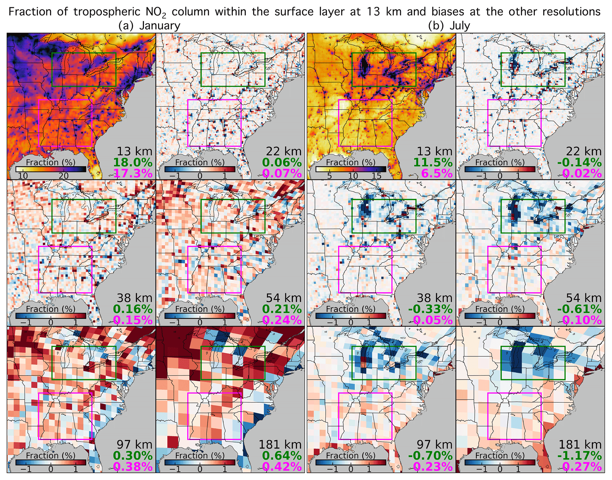
Figure 6 Coarse-resolution simulations yield variable biases in satellite-based estimations of surface NO₂ concentration. Panels (a) and (b) are both similar to Fig. 1c (for January and July 2015, respectively) but for the fraction (%) of NO₂ tropospheric column within the surface layer during afternoon satellite overpass time (19:00–21:00 UTC). The numbers for the other resolutions vs. 13 km resolution are absolute differences in percentage number.

Figure 7 shows the simulated tropospheric NO₂ vertical column density (Ω) and its resolution dependence during LEO afternoon overpass time, and Fig. A5 shows the corresponding slant column density (Ω_s) after applying TROPOMI scattering weights. Relative to the surface biases (Fig. 1c), the Ω and Ω_s differences show stronger regional uniformity, revealing overall increasingly negative biases with increasing grid size over both seasons and regions. For July and over the SS, the afternoon columnar biases are reversed to be negative compared to the positive surface biases (e.g., Fig. 7 vs. Fig. 1c), driven by the reversed responses at higher altitudes (Fig. 4). This remarkable reversal of Ω biases (negative) vs. surface biases (positive) reinforces the need to include vertical profile information to correctly simulate NO_x columnar properties. Ω and Ω_s exhibit quantitatively consistent resolution dependence and spatial distribution (Fig. 7 vs. Fig. A5), indicating that the changes in vertical profile do not significantly alter the resolution dependence of satellite-observed columnar abundances compared to the direct effects from changing τ. Assuming NO_x emissions are locally related to NO₂ columns at coarse resolution will result in similar magnitudes of overprediction (up to 8 % and 4 % over the GL and SS, respectively, in July) of derived NO_x emissions to compensate the underestimated Ω to emission relationship under an inverse modeling framework configured at each resolution, as shown in Figs. 7 and A5.

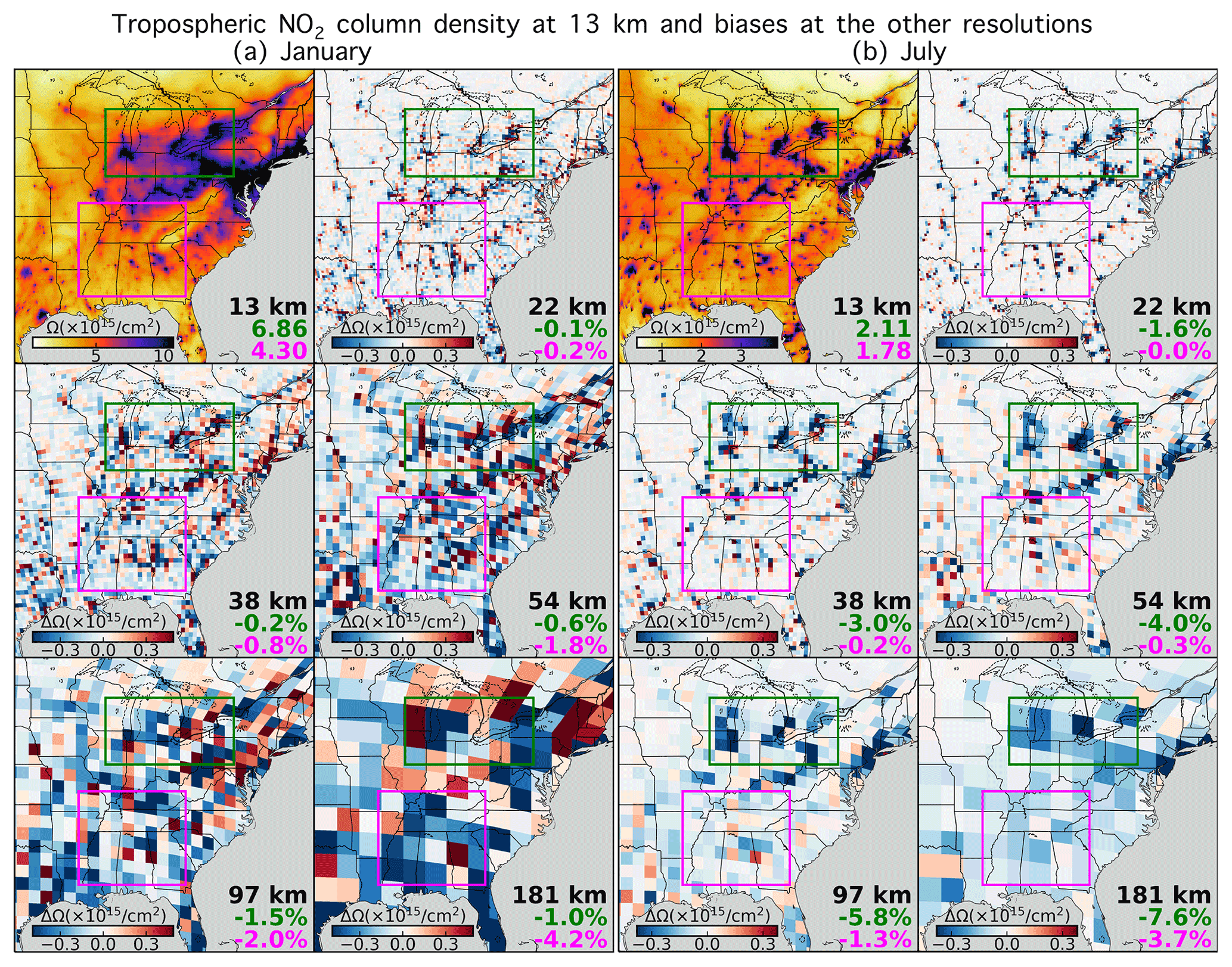
Figure 7 Coarse-resolution simulations yield positive biases in spaceborne inverse modeling of NO_x emissions. Panels (a) and (b) are both similar to Fig. 1c (for January and July 2015, respectively) but for the mean GEOS-Chem tropospheric NO₂ column density (in molec. cm⁻²) during afternoon satellite overpass time (19:00–21:00 UTC).

4 Discussions and conclusions

The strong, and more importantly regionally variable, NO_x resolution dependences that we find in the lower troposphere over the contemporary eastern US warrant care in interpreting coarse-resolution NO_x simulations. We find that resolution-dependent NO_x biases are particularly pronounced at the surface in summer, with variable effects seasonally, regionally, diurnally and vertically, which also affect remote sensing observations interpreted with low-resolution simulations. At daytime with strong photochemistry, higher-resolution modeling more realistically concentrates NO_x emissions near sources, thus decreasing τ in the NO_x-limited regime and increasing τ in the NO_x-saturated regime (Fig. A1). Existing literature about NO_x resolution dependencies in box models (Valin et al., 2011), at power plants (Sillman et al., 1990), in ship plumes (Charlton-Perez et al., 2009) and in CTMs (Wild and Prather, 2006; Yamaji et al., 2014; Yan et al., 2016) primarily discusses the NO_x-saturated regimes. We find limited prior literature about the positive biases of NO_x over weak sources (i.e., in the NO_x-limited regime over the SS) in CTM simulations. The lack of similar prior reports reflects the chemical regime transition occurring in the last ∼ 10 years, while typical point sources were previously predominantly in the NO_x-saturated regime. Attention to the NO_x-limited regime and its corresponding resolution effects is timely given declining NO_x emissions across the US with NO_x emission regulations. At the same time, the joint sensitivity to NO_x heterogeneity and concurrent VOC level (Sect. 3.1) in the NO_x-limited regime will continue complicating its predictability, since NO_x and VOCs can have various spatial co-variabilities (e.g., positively correlated where transportation-relevant VOCs and NO_x both dominate) and regime-dependent effects on τ. Therefore, accurately capturing such regime differences and transitions from CTM requires not only accurate emission inventories of NO_x and VOC but also simulations at representative spatial scales (e.g., 10 km or finer) that correctly distribute these emissions (Valin et al., 2011).

We found systematic resolution effects of nighttime NO–O₃ titration efficiency that can drive the NO_x biases over winter (Fig. 2 and Sect. 3.2), as the anti-correlation between NO and O₃ implies faster reaction rates at coarser resolutions. In air quality modeling, many key reactions involve spatially correlated (e.g., co-emitted SO₂ and NO₂ cause severe urban haze (Wang et al., 2020)) or segregated species (e.g., agricultural NH₃ and NO_x-formed HNO₃ for nitrate aerosol partitioning (Gu et al., 2021)). Like in this study, the segregated species will consume precursors and produce products more efficiently at coarser resolutions, while colocated sources will experience opposite effects. Interpreting the evolution of relevant species and air pollution processes using a CTM is therefore also preferable at the spatial scales that are representative of these sources. This effect should also be taken into account when CTMs are simulated on coarser scales.

Our detailed simulation of resolution effects at different altitudes (Figs. 4 and 5) revealed vertically variable sensitivity of NO_x to its chemical loss at different spatial resolutions. These findings significantly enriched the understanding of resolution dependency of satellite columnar observations, which is in contrast to previous studies that neglected vertical layering. The example of the opposite resolution effect of Ω and surface NO_x (Fig. 7 vs. Fig. 1c) over the SS in July highlights the necessity of realistic vertical profiling of NO_x and its chemical sinks. For two conventional applications of satellite-retrieved Ω, namely estimation of surface NO₂ concentration and constraining NO_x emissions, we found that regionally and seasonally varying biases at the level of ∼ 10 % due to adopting coarse model simulations (∼ 200 km) are inevitable.

Overall, we conducted a comprehensive novel evaluation of NO_x resolution dependence using a CTM across a wide range of resolutions (13–181 km) and scenarios (including nighttime, winter and higher altitudes). We found the strongest resolution effects in the summer and during daytime (e.g., −16 % for surface NO_x and −8 % for columnar NO₂ over the GL) where and when the NO_x spatial heterogeneity is the strongest and its lifetime is the shortest (e.g., Fig. S2). We attribute these systematic simulation biases mainly to the strong localization of NO_x emission and chemistry at a spatial scale of ∼ 10 km and below. Additional modulations from other factors across resolutions, such as sub-grid meteorology-relevant processes (e.g., transport) are also possible but are fully coupled with the feedbacks revealed in this paper and are non-trivial to disentangle. These systematic resolution dependences should be considered when constraining model parameters (e.g., emissions, reaction yields, removal rates) using ground- or satellite-based observations. In other words, relevant interpretations and conclusions by coarse-model simulations in previous studies are worth revisiting. For example, NO_x sources and sinks constrained by matching inadequately coarse simulations with observations could be biased to compensate for the intrinsic model errors discussed here.

Although this study exploited state-of-science capabilities, biases with respect to resolutions finer than 13 km resolution likely exist considering the highly localized NO_x, especially in summer (Valin et al., 2011; Larkin et al., 2017; Beirle et al., 2019). Following NO_x regulations in the US, the magnitudes of resolution effects are expected to continue decreasing as the enhancements over sources reduce relative to the background NO_x level (Russell et al., 2012; Jin et al., 2020; Qu et al., 2021), and the requirements regarding resolution may diminish (e.g., partially reflected by the smaller effects over the SS relative to over the GL). Nonetheless, over developing areas where current NO_x emissions are stronger or are projected to increase, the resolution effects will be exacerbated, and applying finer-resolution simulations to accurately capture NO_x lifetime and budgets will be increasingly critical for air quality modeling applications. Optimization of an appropriate resolution that can capture the relevant processes accurately for specific applications given computational resource constraints is also of great interest. GCHP offers this global high-resolution simulation capability and also the opportunity to expand this analysis into a more comprehensive understanding of the global resolution dependence of NO_x and its nonlinear chemistry.

Appendix A: Complementary figures to assist interpretation

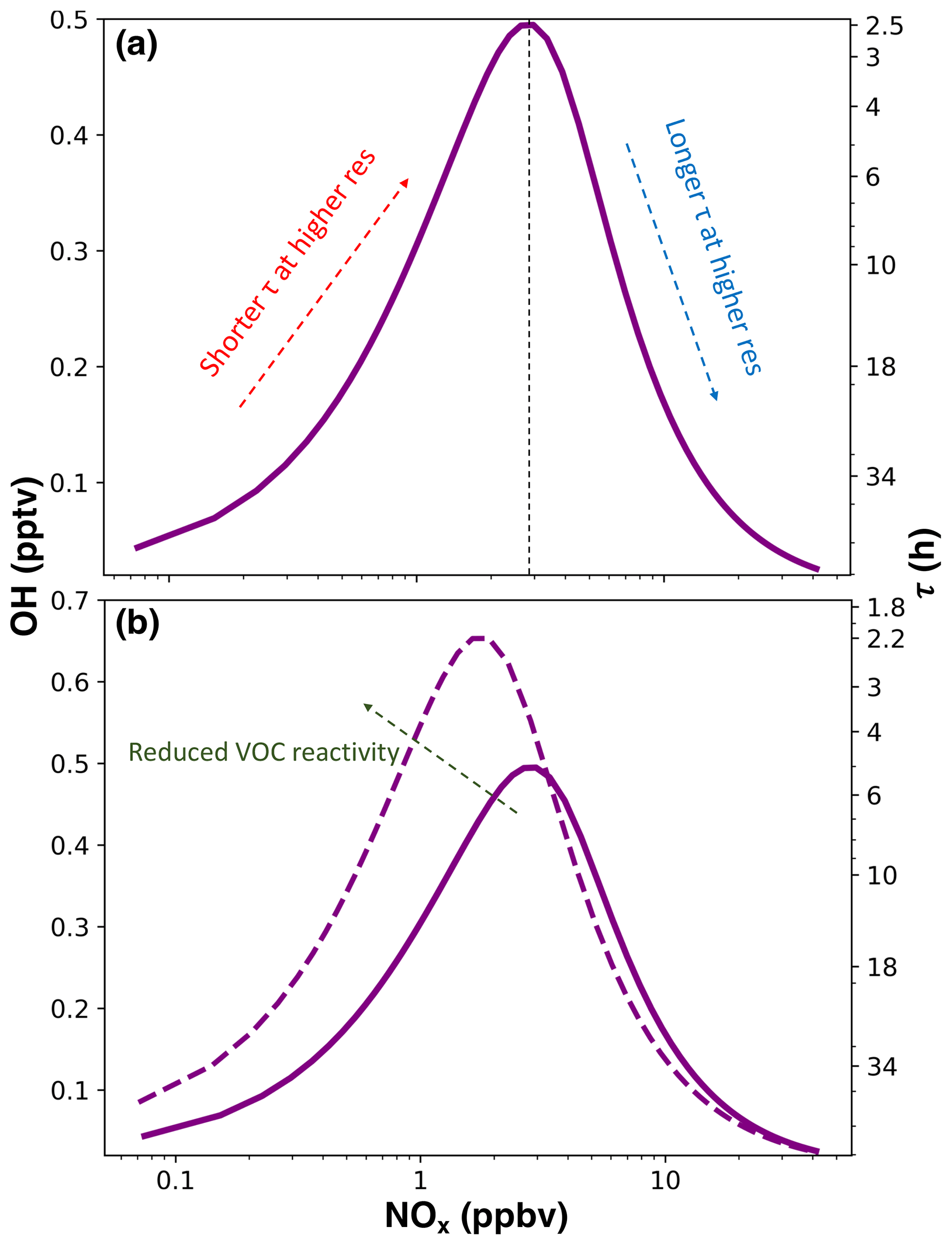
Figure A1 (a) Illustration of the daytime NO_x–OH lifetime feedback. Higher-resolution modeling tends to concentrate the most NO_x emissions near sources, thus will decrease NO_x lifetime in the NO_x-limited regime (left) and increase NO_x lifetime in the NO_x-saturated regime (right). The steady-state concentrations were calculated assuming a ${\mathrm{NO}}_{\mathrm{2}}/\mathrm{NO}$ ratio of 4, an alkyl nitrate branching ratio of 0.04, a VOC reactivity of 3 s⁻¹ and an initial ozone concentration of 25 ppb, and the production of HO_x is proportional to ozone. Panel (b) is the same as (a) but including an additional scenario where the VOC reactivity is reduced by 50 % (dashed).

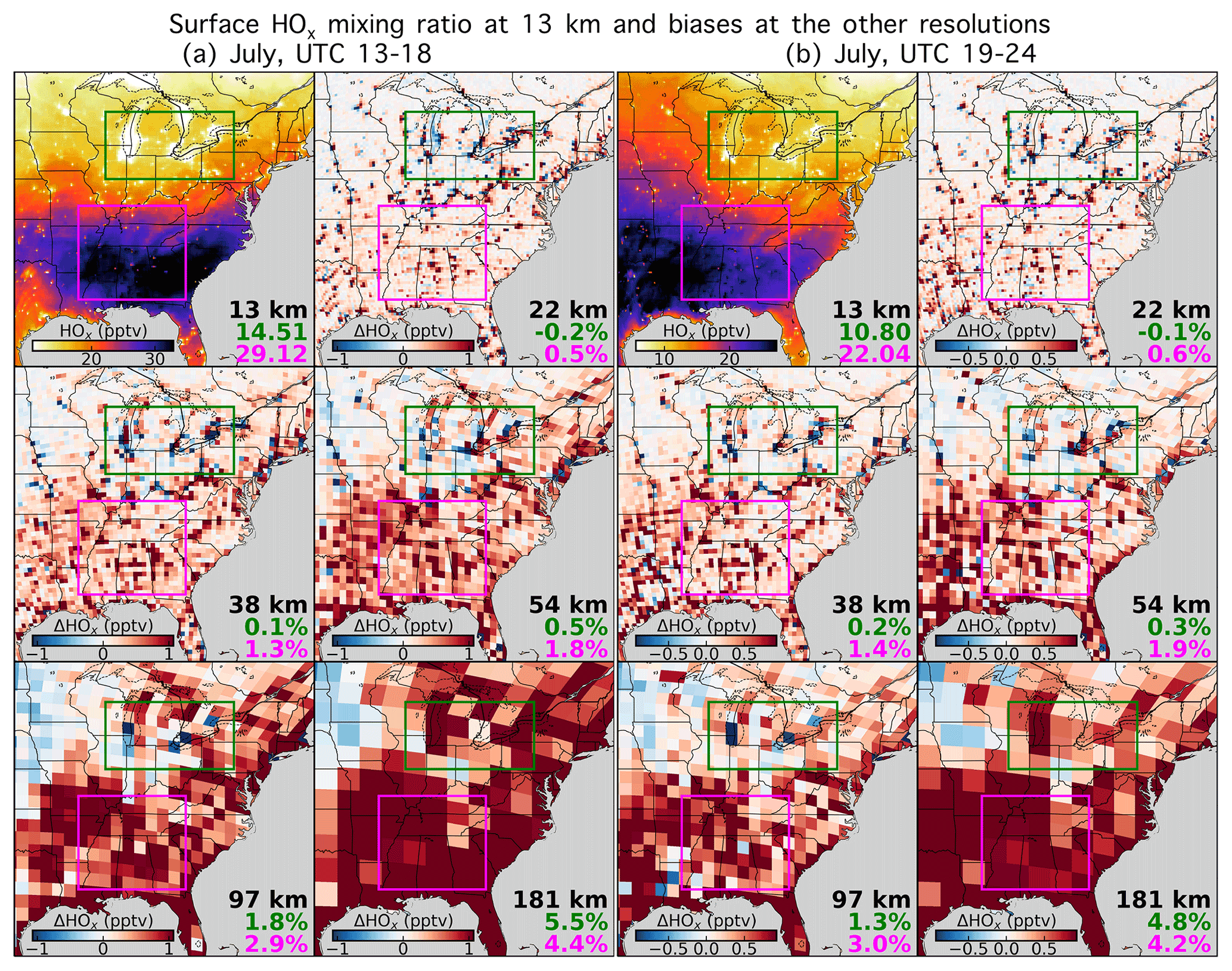
Figure A2 Similar to Fig. 1c but for HO_x in the morning (a 13:00–18:00 UTC or 07:00–12:00 CST) and afternoon (b 19:00–24:00 UTC or 13:00–18:00 CST), respectively.

Figure A3 Similar to Fig. 1c but for morning (13:00–18:00 UTC or 07:00–12:00 CST) NO_x.

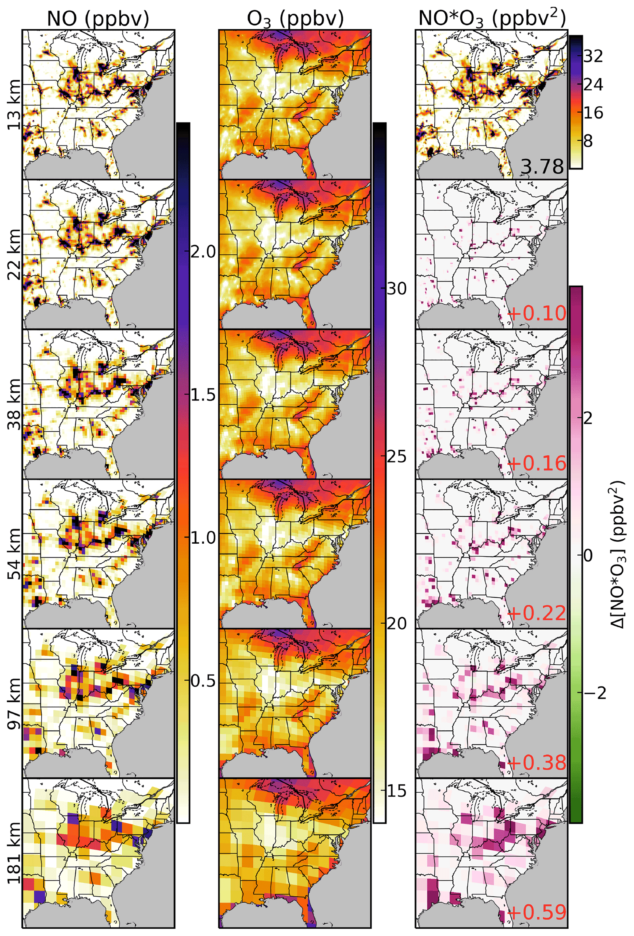
Figure A4 Illustration of the resolution-dependent nighttime NO–O₃ titration efficiency. The left and middle columns are mean surface NO and O₃ concentration at 00:00 UTC+6 in January 2015 at 13 km (top row) and regridded to the other resolutions. The right column shows their products at 13 km resolution and their differences if calculated at the other coarser resolutions. Domain mean products and differences are shown as an inset.

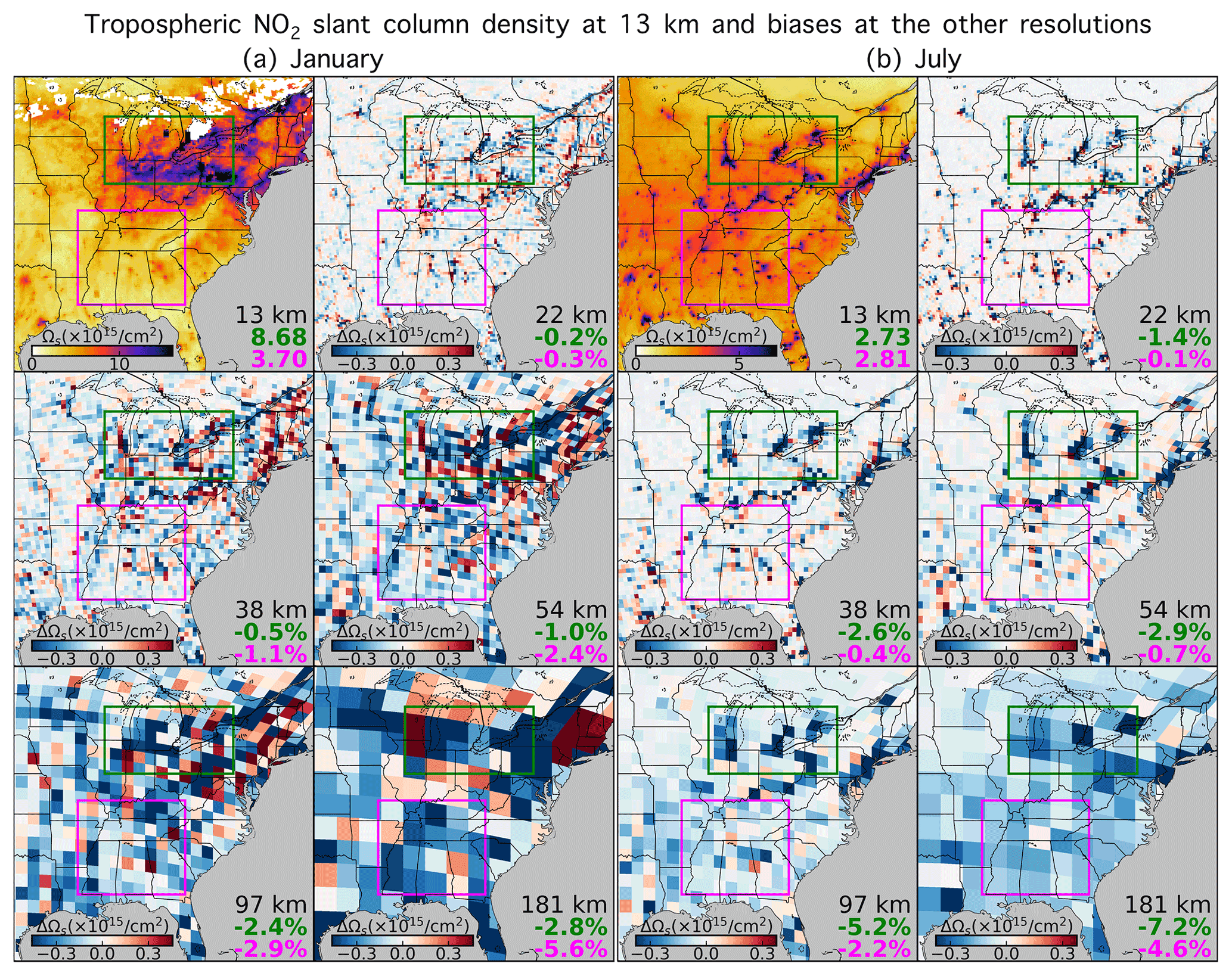
Figure A5 Similar to Fig. 7 but for slant column density (Ω_s, molec. cm⁻²) calculated from GEOS-Chem NO₂ mixing ratios and scattering weights corresponding to TROPOMI observations. The small blank (white) areas in January have no available TROPOMI retrievals under clear-sky and snow-free conditions.