the Creative Commons Attribution 4.0 License.
the Creative Commons Attribution 4.0 License.
 | 07 Mar 2023
Measurement report: Production and loss of atmospheric formaldehyde at a suburban site of Shanghai in summertime
Yizhen Wu
Juntao Huo
Gan Yang
Yuwei Wang
Lihong Wang
Shijian Wu
Formaldehyde (HCHO) is an important trace gas that affects the abundance of HO2 radicals and ozone, leads to complex photochemical processes, and yields a variety of secondary atmospheric pollutants. In a 2021 summer campaign at the Dianshan Lake (DSL) Air Quality Monitoring Supersite in a suburban area of Shanghai, China, we measured atmospheric formaldehyde (HCHO) by a commercial Aero-Laser formaldehyde monitor, methane, and a range of non-methane hydrocarbons (NMHCs). Ambient HCHO showed a significant diurnal cycle with an average concentration of 2.2 ± 1.8 ppbv (parts per billion by volume). During the time period with the most intensive photochemistry (10:00–16:00 LT), secondary production of HCHO was estimated to account for approximately 69.6 % according to a multi-linear regression method based on ambient measurements of HCHO, acetylene (C2H2), and ozone (O3). The average secondary HCHO production rate was estimated to be 0.73 ppbv h−1 during the whole campaign (including daytime and nighttime), with a dominant contribution from reactions between alkenes and OH radicals (66.3 %), followed by OH-radical-initiated reactions with alkanes and aromatics (together 19.0 %), OH-radical-initiated reactions with oxygenated volatile organic compounds (OVOCs; 8.7 %), and ozonolysis of alkenes (6.0 %). An overall HCHO loss, including HCHO photolysis, reactions with OH radicals, and dry deposition, was estimated to be 0.49 ppbv h−1. Calculated net HCHO production rates were in relatively good agreement with the observed rates of HCHO concentration change throughout the sunny days, indicating that HCHO was approximately produced by oxidation of the 24 hydrocarbons we took into account at the DSL site during the campaign, whereas calculated net HCHO production rates prevailed over the observed rates of HCHO concentration change in the morning/midday hours on the cloudy and rainy days, indicating a missing loss term, most likely due to HCHO wet deposition. Our results suggest the important role of secondary pollution in the suburbs of Shanghai, where alkenes are likely key precursors for HCHO.
- Article
(10400 KB) - Full-text XML
-
Supplement
(610 KB) - BibTeX
- EndNote


Formaldehyde (HCHO) is the most abundant carbonyl in the troposphere, is an intermediate product from the oxidation of various volatile organic compounds (VOCs), and plays an important role in various photochemical processes as both a source and a sink of free radicals (Wittrock et al., 2006). Photolysis of HCHO produces HO2 radicals that can be subsequently converted to OH radicals, altering the oxidative capacity of the atmosphere (Mahajan et al., 2010; Tan et al., 2019a). HCHO can also contribute to ozone (O3) formation, and their link is one of the most popular topics of atmospheric research (Hong et al., 2022; Liu et al., 2007; Pavel et al., 2021). Furthermore, HCHO can play a crucial catalytic role in the formation of particulate matter via in-cloud processing pathways to form hydroxymethyl hydroperoxide (HMHP) or hydroxymethanesulfonate (HMS) (Dovrou et al., 2022). Additionally, HCHO has adverse health effects on humans and animals, possibly causing respiratory and cardiovascular diseases (Zhu et al., 2017).
Direct emission of HCHO can be attributed to anthropogenic activities, such as vehicle exhaust, industrial emissions, and fossil fuel combustion, and thus primary HCHO is closely related to anthropogenic pollutants such as acetylene (C2H2), carbon monoxide (CO), nitrogen oxidizes (NOx), and traffic-related black carbon (BC) (de Gouw et al., 2005; Zhang et al., 2013; Dutta et al., 2010; Possanzini et al., 2002; Lin et al., 2012). Observations in city centers usually showed important HCHO sources of direct anthropogenic emissions (Dutta et al., 2010; Possanzini et al., 2002; Lin et al., 2012). On the other hand, previous studies have indicated that secondary production of HCHO plays an important role in remote areas; HCHO comes from complex oxidation processes of a wide range of VOCs by ubiquitous atmospheric oxidants like OH radicals and O3 (Lin et al., 2012; Anderson et al., 2017; Nussbaumer et al., 2021). Especially in summertime, increases in temperature are always linked with higher solar radiation and larger biogenic isoprene emission, which have been proved to jointly contribute to the higher abundance of HCHO (Choi et al., 2010; Sumner et al., 2001; Wang et al., 2017). Due to the short lifetime of HCHO, primary emissions and transport processes are important in source regions but can be mostly neglected in remote locations. On the other hand, secondary HCHO production paths are more diverse and complex, and thus they are difficult to be quantified.
In previous studies, several methods were used to separate the primary and secondary sources of HCHO, including the emission ratios of HCHO to tracers from primary sources (Possanzini et al., 2002; Lin et al., 2012); the photochemical-age-based parameterization (de Gouw et al., 2005, 2018; Wang et al., 2017); receptor models such as the positive matrix factorization (PMF) model and the principal component analysis (PCA) model (Wang et al., 2017; Chen et al., 2014); and the multi-linear regression method based on ambient measurements of HCHO and various tracers that can represent primary and secondary sources, respectively (Su et al., 2019; S. Zhang et al., 2021). These methods just provide a simple estimation on the ratios of different HCHO sources. Nevertheless, contributions of different precursors are the key to understanding and preventing HCHO production, but a qualitative and quantitative understanding of the HCHO production and loss is still incomplete.
HCHO sources have been previously studied in China (Xing et al., 2020; Su et al., 2019; Wang et al., 2017; Sun et al., 2021; S. Zhang et al., 2021), whereby general fractions of primary and secondary HCHO were provided, and important roles of secondary HCHO sources were suggested. Primary and secondary contributions to ambient HCHO were separated using a multiple linear regression based on HCHO observed by the Ozone Mapping and Profiler Suite (OMPS) in the Yangtze River Delta in China, suggesting that secondary formation, especially photochemical production, played crucial roles (Su et al., 2019; S. Zhang et al., 2021). A more recent study used the GEOS-Chem model to stimulate the concentrations of HCHO over Hefei Province in summer, indicating that oxidations of both methane and non-methane VOCs dominated the HCHO production with a contribution of 43.27 % and 56.73 %, respectively (Sun et al., 2021). To the best of our knowledge, little has been done to quantify the contributions of various specific precursors to HCHO production in China.
On the other hand, studies that have estimated the secondary HCHO production and discriminated the contribution of different secondary HCHO precursors in North America and Europe still found missing production terms (Lin et al., 2012; Sumner et al., 2001). For example, missing HCHO production rates of 1.1–1.6 ppbv h−1 were reported for a remote site in America, which was nearly double the calculated secondary production rates (Choi et al., 2010). Moreover, very few studies have evaluated the HCHO budget by comparing the net production of HCHO (P(HCHO) − L(HCHO)) and the observed rates of HCHO concentration change, and even for those with such attempts, discrepancies remained (Sumner et al., 2001; K. Zhang et al., 2021). Therefore, an estimation of secondary HCHO production based on a comprehensive observation of HCHO precursors, as well as a comprehensive understanding of the formation and loss of HCHO to fill the gap in the HCHO budget calculation, is urgently needed to reveal the key precursors to HCHO formation, especially in eastern China, where photochemical pollution has become severe in recent years.
In this study, we measured atmospheric HCHO concentrations using a commercial Aero-Laser formaldehyde monitor from 10 June to 4 July 2021 at the Dianshan Lake (DSL) Air Quality Monitoring Supersite, a suburban area of Shanghai. The secondary HCHO production rates were estimated based on parallel measurements of O3, photolysis frequencies, and 24 VOCs whose photochemical reactions lead to formation of HCHO. The loss of HCHO, including HCHO photolysis, reactions with OH radicals, and dry deposition, was estimated. Also, characteristics of secondary HCHO production between the sunny period and the cloudy and rainy period were compared. Lastly, the calculated net HCHO production rates were compared with the observed rates of HCHO concentration change.
2.1 Measurement site
A comprehensive campaign was carried out at the DSL Air Quality Monitoring Supersite in Shanghai, China (31.10∘ N, 120.98∘ E), covering 10 June to 4 July 2021. The station is located in Qingpu District in a western suburb of Shanghai, about 37 km away from the city center, and it is surrounded by Dianshan Lake and several villages with few residents (Fig. 1). There is a high road (G318) about 0.4 km southeast of the sampling site. Since it is located at the junction of Shanghai, Zhejiang Province, and Jiangsu Province, all of which are well-developed areas with large populations, this super site is often affected by regional transport and suffers from photochemical pollution episodes (Yang et al., 2022).
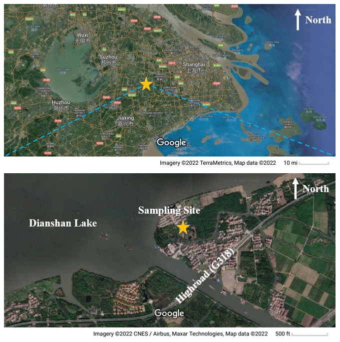
Figure 1A topography map (from © Google Maps) of the region around the Dianshan Lake (DSL) Air Quality Monitoring Supersite (31.10∘ N, 120.98∘ E).
2.2 Measurements of VOCs
Atmospheric HCHO was measured by a commercial Aero-Laser formaldehyde monitor (Aero-Laser GmbH, model AL4021) with a detection limit (DL) of 100 pptv (parts per trillion by volume). In this instrument, gaseous HCHO is firstly absorbed by sulfuric acid (0.3 %) and transferred into liquid phase, and then the aqueous HCHO reacts with acetylacetone and ammonia to produce 3,5-diacetyl-1,4-dihydrolutidine (DDL), which can be excited by a laser at 410 nm, and the fluorescence at 510 nm is used to quantify HCHO. Liquid formaldehyde standards of 80 µg L−1 were used to calibrate the instrument weekly. HCHO was measured at a time resolution of 5 min, but the obtained data were processed at 1 h intervals to match the VOC data from the online gas chromatograph equipped with mass spectrometry and flame ionization detection (GC–MS/FID) system.
Atmospheric methane was measured with GC–FID (ChromaTHC, model C24022). Methane was separated from ambient non-methane hydrocarbons (NMHCs), since NMHCs were concentrated in a packed stainless-steel column filled with Porapak Q, 50/80 mesh, whereas methane was able to freely pass the column and be detected by a hydrogen ion flame detector. Methane standards of 2 ppmv (parts per million by volume) were used to perform instrument calibration every week, and those at five concentration levels (0, 1, 2, 3, 4 ppmv) were used to quantify the concentration of ambient methane. The concentration of methane was detected at a time resolution of 5 min but averaged at 1 h intervals to match the GC–MS/FID data.
Sampling of Photochemical Assessment Monitoring Station (PAMS) VOC compounds were performed for 10 min each hour, and the resulting data from GC–MS/FID (TH-PKU 300B) analysis were used to represent concentrations of PAMS compounds in that hour, given the time for heating and cooling of the GC oven (Li et al., 2015). This practice may miss spikes of PAMS concentration variation, but on a longer timescale, the general characteristics of ambient air composition and concentrations likely still show similar features in 1 h (Kumar and Sinha, 2014; Li et al., 2015; Yuan et al., 2012; Yang et al., 2022). Ambient concentrations of 2-methyl pentane were always below the detection limit of this compound in the instrument, and thus the corresponding data were not included. Ambient air was sampled into the system, where C2–C5 hydrocarbons were separated by a porous-layer open-tubular (PLOT) column (Agilent Technologies Inc.) and measured by the FID channel, and the other hydrocarbons (C6–C12) were preconcentrated by a semi-polar column (DB-624, Agilent Technologies Inc.) and detected using a quadrupole MS detector. Weekly calibration was conducted by a built-in auto-calibration system, using gaseous bromochloromethane, 1,2-difluorobenzene, chlorobenzene-d5, and bromofluorobenzene in high-purity N2, each of which is of 4 ppbv. Mixtures of 57 PAMS compounds at 5 concentration levels (0, 1, 2, 4, 8 ppbv) were used to quantify the ambient concentrations of these species.
Isoprene, alpha-pinene, methyl vinyl ketone (MVK), and methacrolein (MACR) were detected by a system consisting of a two-channel gas chromatograph with an electron ionization time-of-flight mass spectrometer (GC–EI-TOF-MS). The GC–EI-TOF-MS system consists of three main components: (1) a thermal desorption pre-concentrator (TDPC) (Aerodyne Research Inc.) for sample collection, (2) a gas chromatograph (GC) (Aerodyne Research Inc.) for sample separation, and (3) an electron ionization time-of-flight mass spectrometer (EI-TOF-MS) (Tofwerk AG, model EI-HTOF) for sample detection (Obersteiner et al., 2016; Claflin et al., 2021). Before pre-concentration, the ambient sample is passed through a bed of pre-cleaned sodium sulfite (nominal 1 g) held in a quartz tube with glass wool packing to scrub ozone and thereby reduce sampling artifacts (Helmig, 1997). The TDPC employed for this campaign relied upon two-stage adsorbent trapping for preconcentration of analytes, using multibed, preconditioned glass sample tubes ( in. o.d.; Markes International), followed by sample focusing on narrow-bore, multibed glass focus traps ( in. o.d.; Markes International). The first stage of trapping allows sampling rates up to 100 sccm, followed by a post-collection purge with dry gas to remove water before focusing; during this campaign, the sample volume was about 800 cm3 per channel. The ARI GC was configured as a two-channel system to expand the volatility range, with a 30 m Rxi-624 analytical column (0.25 mm i.d., 1.4 µm film thickness; Restek) for Channel 1 and a 30 m MXT-WAX analytical column (0.25 mm i.d., 0.25 µm film thickness; Restek) for Channel 2. Isoprene, alpha-pinene, MVK, and MACR were all analyzed on the Rxi-624 column, which ran a ramped temperature program optimized for C5–C12 hydrocarbons, along with oxygen-, nitrogen-, halogen-, and sulfur-containing VOCs. Automated gas-phase calibration and instrument background measurements of GC–EI-TOF-MS were conducted every 20 h with a standard gas cylinder (Apel-Riemer Environmental Inc.), including MVK, furan, propanal, methyl tert-butyl ether, butanal, ethyl acetate, toluene, octane, m-xylene, o-xylene, naphthalene, 1-methylnaphthalene, decamethylcyclopentasiloxane, and limonene. MVK was calibrated during the campaign with the automated gas-phase calibration as mentioned above. Isoprene and alpha-pinene were calibrated after the campaign using another calibrant cylinder (Weichuang Standard Reference Gas Analytical Technology Co., Ltd.), where a five-point calibration was conducted, and each point was repeated three times. As for MACR, calibration was conducted after the campaign with a liquid calibration system (LCS; Tofwerk AG). Briefly, liquid MACR was diluted with methanol and injected steadily into a stream of 2 slpm (standard liters per minute) ultra-high-purity N2 with a high-precision syringe pump, part of which (around 198 sccm) was guided into the GC–EI-TOF-MS. The sampling time of the GC–EI-TOF-MS was adjusted to obtain a four-point calibration curve with three duplicates for each point. The consistency between the liquid calibration and the calibrant cylinder calibration was confirmed by conducting both calibration methods for m-xylene, o-xylene, 1,2,4-TMB, and benzene. The sensitivity of the GC–EI-TOF-MS during and after the campaign was calibrated and normalized using the first standard gas cylinder (Apel-Riemer Environmental Inc.). Concentrations of isoprene, alpha-pinene, MVK, and MACR were measured with a time resolution of 30 min and were later averaged at 1 h intervals to match the GC–MS/FID data.
Isoprene was detected by both GC–MS/FID (DL of 0.04 ppbv for isoprene) and GC–EI-TOF-MS (DL of 0.77 pptv), and the corresponding intercomparison is shown in Fig. S1 in the Supplement. Daytime isoprene concentrations showed excellent agreement between two systems (Fig. S1a), whereas at nighttime, GC–MS/FID usually showed higher results than GC–EI-TOF-MS when concentrations of isoprene declined to low values, as shown in Fig. S1b. The reason for the discrepancy at night is unknown. Considering the lower detection limit and higher accuracy of GC–EI-TOF-MS, isoprene measured by GC–EI-TOF-MS is used in the following discussion. The good correlation between daytime isoprene concentrations suggests minor uncertainties in our daytime isoprene concentrations. Though there was a discrepancy between nighttime isoprene concentrations, the concentrations of measured isoprene and estimated OH radicals at night were so low that they hardly affect our results of calculated secondary HCHO production rates.
2.3 Measurements of other pollutants and meteorological parameters
O3 was measured with an ultraviolet photometric analyzer (Thermo Environmental Instruments, TEI Inc., model 49i) with a DL of 1 ppbv (at a time interval of 10 s). NO and NO2 mixing ratios were determined using a chemiluminescent analyzer (TEI, model 42i), the DL for which is 0.40 ppbv (at a time interval of 60 s).
Photolysis frequencies of HCHO, NO2, NO3, O1D, HONO, and H2O2 were determined with an ultra-fast charge-coupled detector (CCD) spectrometer (UF-CCD; Metcon), with a time resolution of 1 min. The instrument consists of an optical receiver, a CCD, and a cooling control box for the detector and covers a spectral band range from 280–650 nm. The photolysis frequencies can be calculated automatically from the measured spectra and the calibration factor, which is obtained from the calibration using NIST/PTB 1000 W halogen lamps.
Temperature (T), relative humidity (RH), atmospheric pressure (P), wind speed (WS), wind direction (WD), and rainfall were captured by an automatic and commercial weather monitoring station (Vaisala AWS310). Boundary layer height (BLH) was recorded by a ceilometer (Vaisala, CL31). Atmospheric parameters were measured at a time resolution of 5 min.
All trace gases, meteorological parameters, and photolysis frequencies were then processed at 1 h intervals to match the GC–MS/FID data.
More details about the detection limit and accuracy of trace gases, VOCs, photolysis frequencies, and BLH can be found in Table S2. Total uncertainties in calculated HCHO production and loss rates were estimated by applying the root square propagation of corresponding uncertainties in quantities used for the calculation.
3.1 Overview of the campaign
This campaign was carried out from 10 June to 4 July 2021 at the DSL site. The sampling period coincided with the plum rain season, a typical East Asian rainy period that features several weeks of wet days as well as high temperatures and usually starts in June, causing a significant weather variation during the campaign.

Figure 2Time profiles of HCHO, Ox (= NO2 + O3), O3, and NOx; photolysis frequencies of O1D (J(O1D)); and meteorological parameters during the campaign.
Figure 2 shows the time profiles of HCHO, Ox (= NO2 + O3), O3, and NOx; photolysis frequencies of O1D (J(O1D)); and meteorological parameters during the campaign. Data points are sometimes missing in the case of routine instrument calibrations and a couple of instrument failures. In addition, Table S1 summarizes the averages and the 10th and 90th percentiles of O3, NO, NO2, C2H2, wind speed, temperature, and relative humidity for the entire campaign and J(O1D), J(HCHO_M), and J(HCHO_R) from sunrise to sunset during the campaign.
J(O1D) showed a normal diurnal variation. The daytime J(O1D) from sunrise to sunset is characterized by an average of 1.23 × 10⁻⁵ s−1 and a 10th and 90th percentile of 1.24 × 10⁻⁶ and 3.08 × 10⁻⁵ s−1, respectively. Ambient temperature was characterized by an average of 26 ∘C and a 10th–90th percentile range of 23–30 ∘C, and RH showed an average of 83 % and a 10th–90th percentile range of 62 %–98 %, which is consistent with the typical features of the plum rain season. The prevailing winds were from the southeast, with an average speed of 1.8 m s−1.
The concentration of O3 was characterized by an average of 31 ppbv and varied between 8–59 ppbv in the 10th–90th percentile range. The 10th–90th percentile concentrations of NO and NO2 were 2–8 and 7–23 ppbv, with average values of 6 and 14 ppbv, respectively. The daily maximum 1 h O3 concentration of 5 d during the campaign exceeded Class I of China National Air Quality Standards (CNAAQS), i.e., an hourly average of 160 µg m−3 (∼ 75 ppbv). Compared with a previous campaign operated at the DSL site in the summer of 2020, where the average concentrations of O3, NO, and NO2 were 37, 4, and 18 ppbv, respectively (Yang et al., 2022), the concentrations of these pollutants in this observation were similar.
HCHO mixing ratios ranged up to the maximum of 9.4 ppbv, with an average value of 2.2 ± 1.8 ppbv (1 standard deviation) and a median value of 1.8 ppbv. The average value was comparable to that (2.2 ppbv) reported in the urban area of New York (USA) in summertime (Lin et al., 2012), but lower than those (5.07 and 5.0 ppbv, respectively) observed in the urban areas of Shanghai (China) and Shenzhen (China) (Ho et al., 2015; Wang et al., 2017). However, the HCHO concentration level at the DSL site was higher than those (1.5, 1.34, 1.1, 1.1, and 0.4 ppbv, respectively) reported in remote areas in the town of Mazhuang (China), Whiteface Mountain (USA), Ineia (Cyprus), Hohenpeißenberg (Germany), and Hyytiälä (Finland) (Wang et al., 2010; Zhou et al., 2007; Nussbaumer et al., 2021).
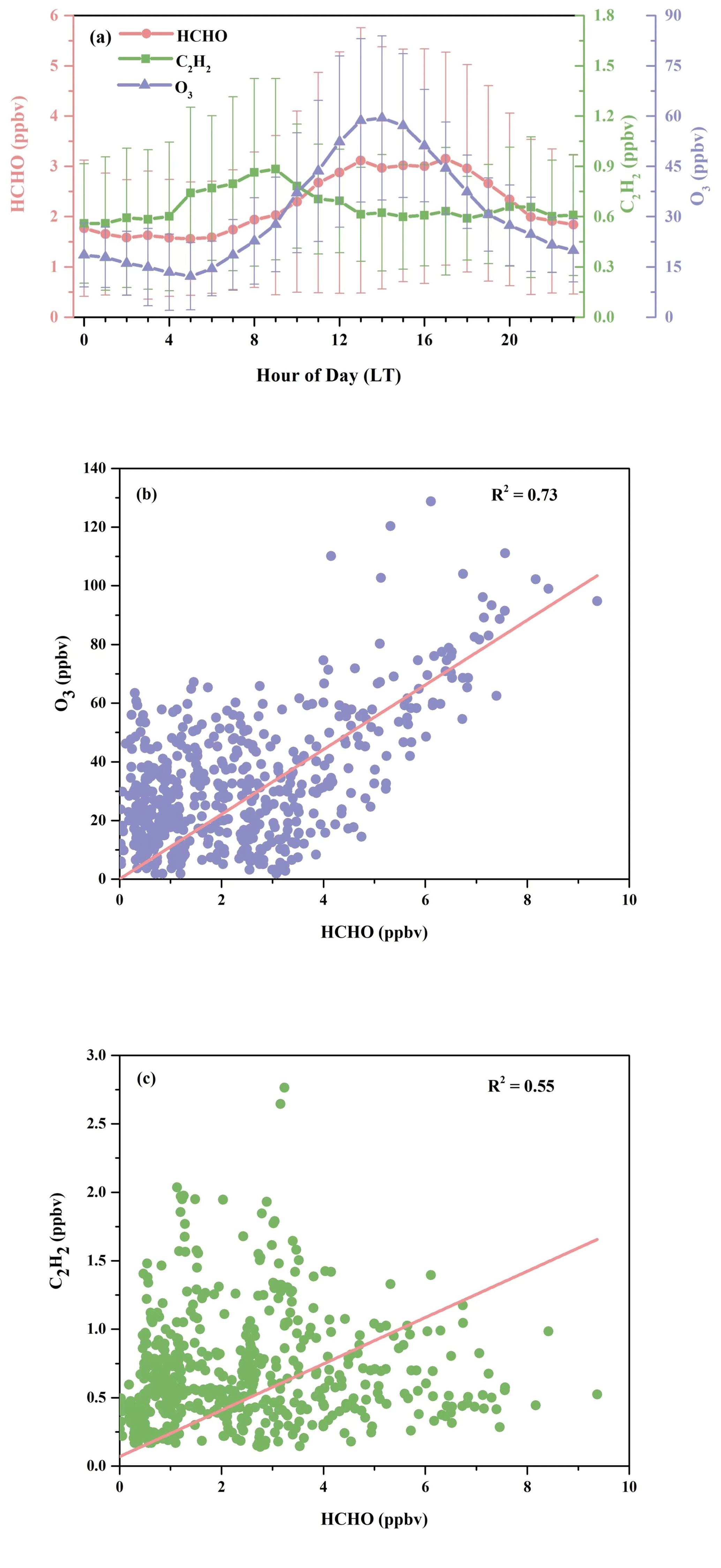
Figure 3(a) Diurnal patterns of HCHO, O3, and C2H2, with the error bar indicating 1 standard deviation; (b) correlation between measured concentrations of HCHO and O3; (c) correlation between measured concentrations of HCHO and C2H2.
In Fig. 2, O3 and Ox show relatively high abundances, while the concentration of traffic-related species like NOx was low. This hints that HCHO at the observation site was potentially associated more with the secondary sources. Figure 3a further illustrates the diurnal variations in HCHO, O3, and C2H2 at the DSL site during the campaign. Both HCHO and O3 exhibited strong diurnal variations during the field measurement, which reached the maximum in the early afternoon, decreased gradually in the afternoon, and remained flat at night. The good correlation between hourly concentrations of HCHO and O3 (R2 = 0.73), as shown in Fig. 3b, indicates important contributions of secondary sources to HCHO. By contrast, the variations in HCHO and C2H2 in Fig. 3a are less parallel. C2H2 increased in the early morning from around 05:00 LT (local time); reached its maximum at rush hour at 08:00–09:00 LT; then decreased till noon and remained relatively steady, with a much smaller peak in the evening around 20:00 LT, which likely coincided with the traffic volumes on the high road. The correlation (R2 = 0.55) between HCHO and C2H2 was lower compared to the correlation between HCHO and O3, as shown in Fig. 3c. These observations roughly indicate that HCHO at the DSL site was more influenced by secondary sources than primary sources.
Here, we present a multi-linear regression method based on measurements of ambient HCHO, C2H2, and O3 to estimate contributions of background, primary, and secondary HCHO. C2H2 is used here as an indicator of primary emissions, whereas O3 is used as a tracer of secondary production. A linear regression model was used to establish a link among the time series of HCHO, C2H2, and O3 (Garcia et al., 2006; S. Zhang et al., 2021; Su et al., 2019; Sun et al., 2021). The observed HCHO can be reproduced by the following linear regression model as shown in Eq. (1).
where β0, β1, and β2 are the fitting coefficients calculated from the multiple linear regression, and [HCHO], [C2H2], and [O3] represent the concentrations of HCHO, C2H2, and O3, respectively. The relative contributions of background, primary, and secondary sources to ambient HCHO can be calculated using Eqs. (2)–(4) (Garcia et al., 2006; S. Zhang et al., 2021; Su et al., 2019; Sun et al., 2021).
where RPrimary denotes the relative contribution of HCHO from primary sources; RSecondary represents the relative contribution of HCHO from secondary sources; and RBackground denotes the relative contribution of background HCHO, which may come from alternated HCHO sources with different residence times or transport of HCHO into the airshed and cannot be classified as primary or secondary sources.
Figure 4 reveals the time series and percentile contributions of background, primary, and secondary HCHO. The modeled HCHO and measured HCHO show a significant linear regression (R = 0.86) (Fig. 4a), which confirms that the multiple linear regression model is statistically reliable. Secondary HCHO dominated local HCHO during the daytime, whereas primary HCHO was more important during nighttime and in the early morning, when photochemical reactions could be nearly neglected (Fig. 4b). The campaign-average relative contributions of secondary production (Fig. 4c) showed the lowest value at 05:00 LT, which was associated with weaker photochemical reactions and higher vehicle emissions due to the morning rush hour. After that, with the increasingly active photochemistry, percentages of secondary HCHO started to rise and reached the peak in the early afternoon (around 13:00–15:00 LT) and then gradually decreased. On average, background, primary, and secondary HCHO contributed 12.7 %, 30.4 %, and 56.9 % to ambient HCHO during the campaign, whereas during the time period with the most intensive photochemistry (10:00–16:00 LT), their relative contributions were 9.5 %, 20.9 %, and 69.6 %, respectively.
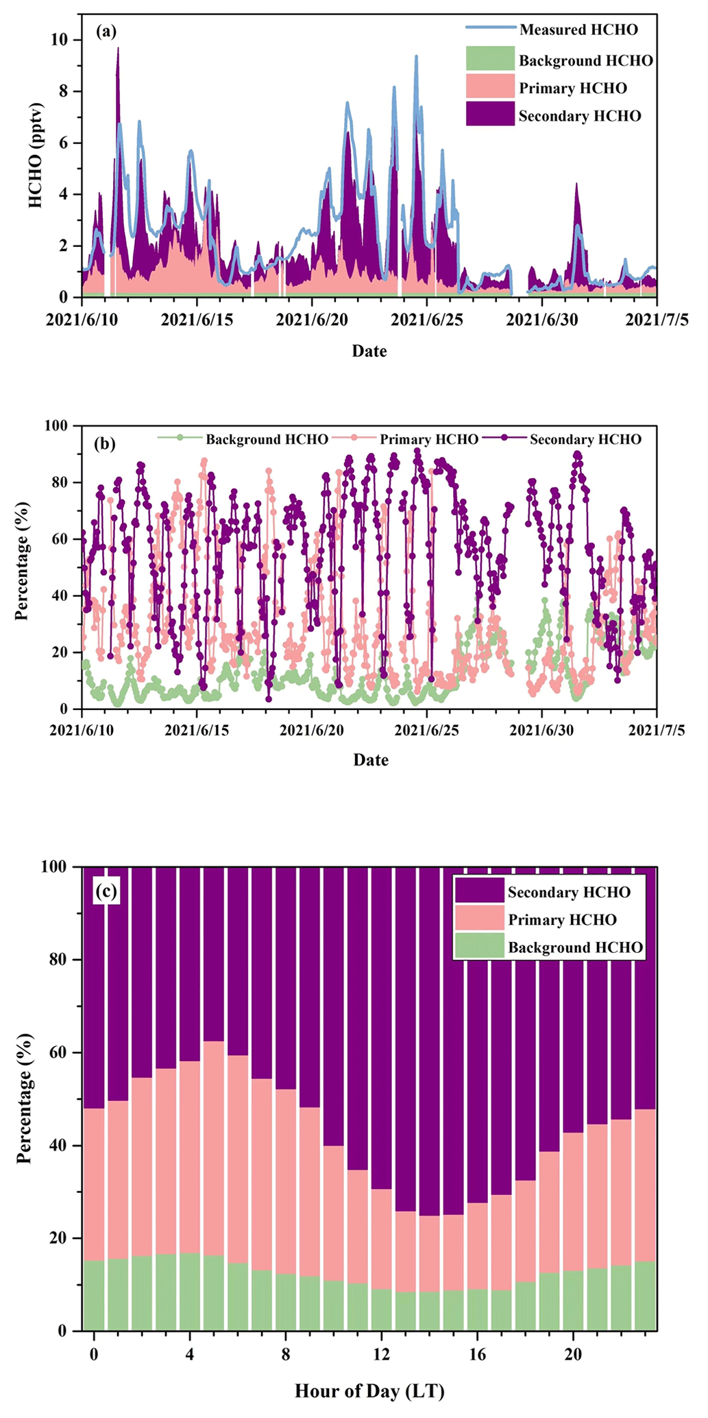
Figure 4(a) Time series and (b) relative contributions of background, primary, and secondary sources to HCHO from a multi-linear regression model during the campaign and (c) campaign-average diurnal contributions of background, primary, and secondary sources.
Another simple method of separating the primary HCHO and secondary HCHO is shown in the Supplement (Sect. S1) for comparison. Diurnal variations in relative contributions of secondary HCHO from two methods are quite similar, as shown in Figs. S2 and 4, though there are tiny differences between the absolute numbers, e.g., 65.7 % according to the ratios of HCHO C2H2 and 69.6 % from the multi-linear regression method, respectively. The estimated contributions of secondary HCHO indicate an important role of secondary HCHO production, especially during the daytime, when the photochemistry is more active.
3.2 HCHO production from VOC oxidation
HCHO is secondarily produced through oxidation of a wide range of atmospheric VOCs by oxidants including OH and O3. Hence, with HCHO yields reported in the literature for these oxidation processes and the concentrations of the parent VOCs and oxidants, the chemical production rate of HCHO can be estimated as shown in Eq. (5) (Lee et al., 1998; Sumner et al., 2001; Choi et al., 2010; Lin et al., 2012).
where i denotes the ith kind of oxidant such as OH or O3; j denotes the jth VOC species that produces HCHO through its oxidation; and kij and γij represent the reaction rate coefficient and the corresponding HCHO yield for the reaction between the ith oxidant and the jth VOC, respectively.
Over 60 VOC species were detected during the campaign, but only 24 VOC species whose oxidation will produce HCHO were used in the calculation of HCHO production rates, including 12 alkanes, 1 aromatic, 9 alkenes, and 2 oxygenated volatile organic compounds (OVOCs). Concentrations of theses 24 VOCs are summarized in Table S3, and the corresponding reaction rate coefficients and HCHO yields taken in the calculation are described in Table S4. The VOC species considered are quite comprehensive, though acetaldehyde, methanol, and methyl hydroperoxide (MHP) are not available in this study. These three compounds, together with acetone, were estimated to account for up to 7 % of secondary HCHO formation at the DSL site, using their concentrations reported in previous studies and that for acetone in our study (Yang et al., 2022; Han et al., 2019; Yuan et al., 2013; Zhang et al., 2012; Nussbaumer et al., 2021). Therefore, we assume their absence would not influence our results considerably.
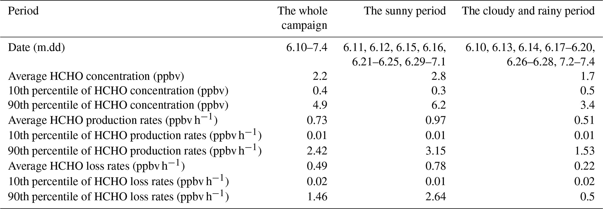
Table 1Comparison of the HCHO concentration, HCHO production rates, and HCHO loss rates between the sunny period and the cloudy and rainy period.
There was not a direct measurement of OH radical concentrations during this campaign, and thus we adopted an empirical equation that has been suggested for OH concentration estimations in four Chinese megacities, including Shanghai, as shown in Eq. (6) (Liu et al., 2020; Tan et al., 2019a; Fan et al., 2021).
where J(O1D) denotes photolysis frequencies of O1D. We compared our calculation results (Table S5) with those from another recommendation (Sect. S2) (Ehhalt and Rohrer, 2000), and their good correlation (R = 0.97) and a slope close to 1 in Fig. S3 validate our estimates. The uncertainties in OH concentration from the calculation were estimated to be 20 %, and this uncertainty was used to estimate those in the production rates and loss rates of HCHO (Tan et al., 2019a; Rohrer and Berresheim, 2006). Figure 5 presents the profile of the calculated HCHO production rates during the whole campaign with a time resolution of 1 h. Overall, alkene oxidation by OH radicals contributed the most to secondary HCHO production, accounting for 66.3 %, followed by OH-radical initiated reactions with alkanes and aromatics (19.0 %) and reactions of OVOCs (8.7 %), while ozonolysis of alkenes contributed 6.0 %, which was the reaction pathway with the smallest contribution. The average calculated secondary HCHO production rate was 0.73 ppbv h−1, with a 90th percentile of 2.42 ppbv h−1 and a 10th percentile of 0.01 ppbv h−1. Peaks of secondary HCHO production rates were usually observed at noon, and the rates showed obvious diurnal cycles. On the other hand, the rates varied significantly during the campaign because secondary HCHO production relies heavily on the weather condition; i.e., photochemical reactions are usually much more active on the sunny days than in the cloudy and rainy period. As we have mentioned before, there were obvious weather variations during the campaign. Therefore, we divided our campaign into the sunny period (including 12 d) and the cloudy and rainy period (13 d) for further investigation. Comparison of the secondary HCHO production between the sunny period and the cloudy and rainy period is shown in Table 1 and Fig. 6.
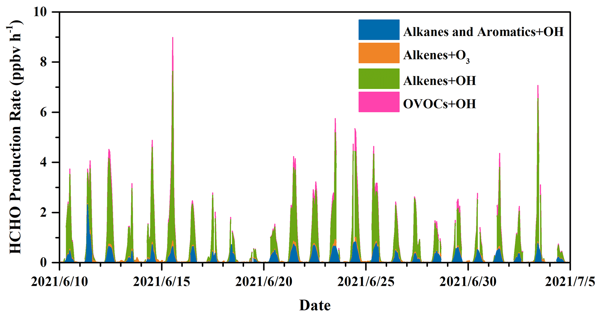
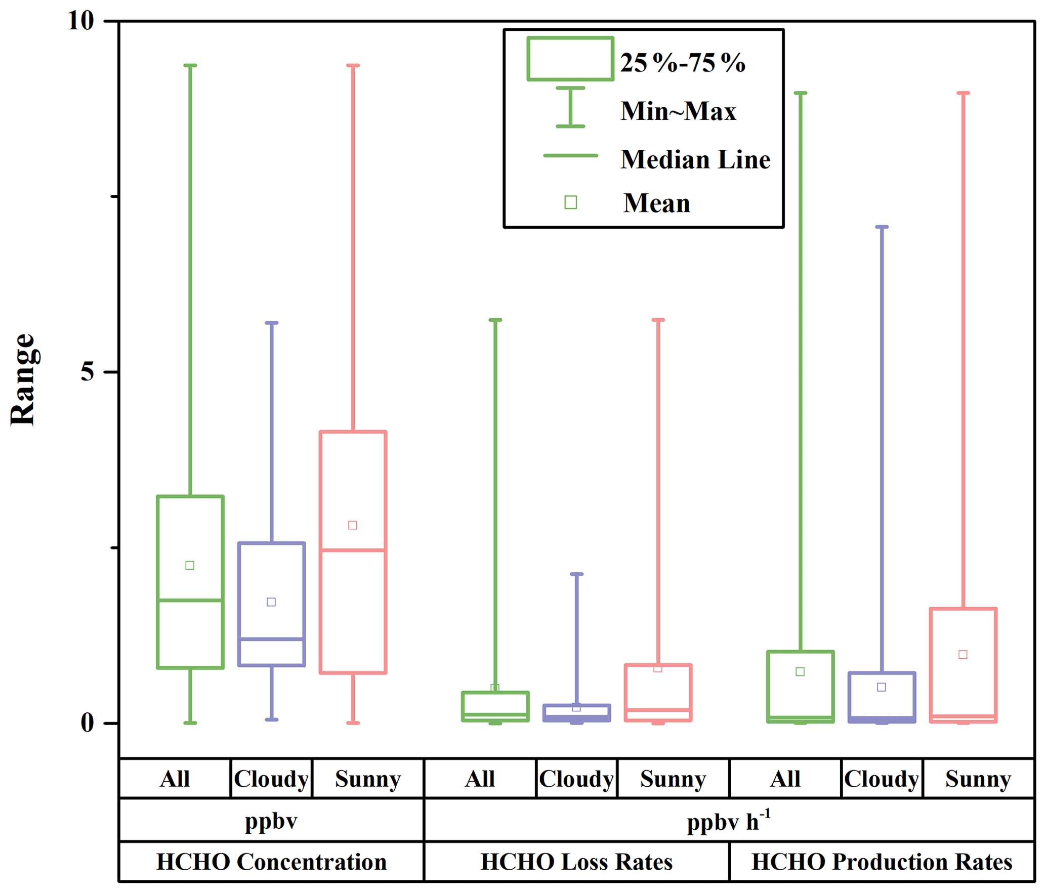
Figure 6Box plots of HCHO concentration, HCHO loss rates, and HCHO production rates during the whole campaign (All), the cloudy and rainy period (Cloudy), and the sunny period (Sunny). The squares represent the mean; the bands inside the box represent the median; the bottom and top of the box represent the lower and upper quartiles, respectively; and the ends of the whiskers show the minimum and the maximum.
In Fig. 7, relative contributions to HCHO production from various processes during the sunny and the cloudy and rainy periods, respectively, are shown, together with the top 10 VOC species that contributed the most in each period, which in total yielded more than 90 % of the overall HCHO. During the sunny days (Fig. 7a), HCHO production was dominated by the reactions of alkenes and OH radicals, accounting for 64.8 %, followed by OH-radical-initiated reactions with alkanes and aromatics (19.5 %), OH-radical-initiated reactions with OVOCs (10.4 %), and ozonolysis of alkenes (5.3 %). As the graph shows, 32.3 % of the secondary HCHO production came from isoprene oxidation (by both OH radical and O3), where OH oxidation of isoprene (30.6 %) dominated. The other main contributors on the sunny days were associated with OH-radical-initiated reactions with ethene (19.4 %), methane (12.9 %), propene (10.6 %), and MVK (8.0 %), which together with isoprene represented more than 80 % of the overall HCHO production.
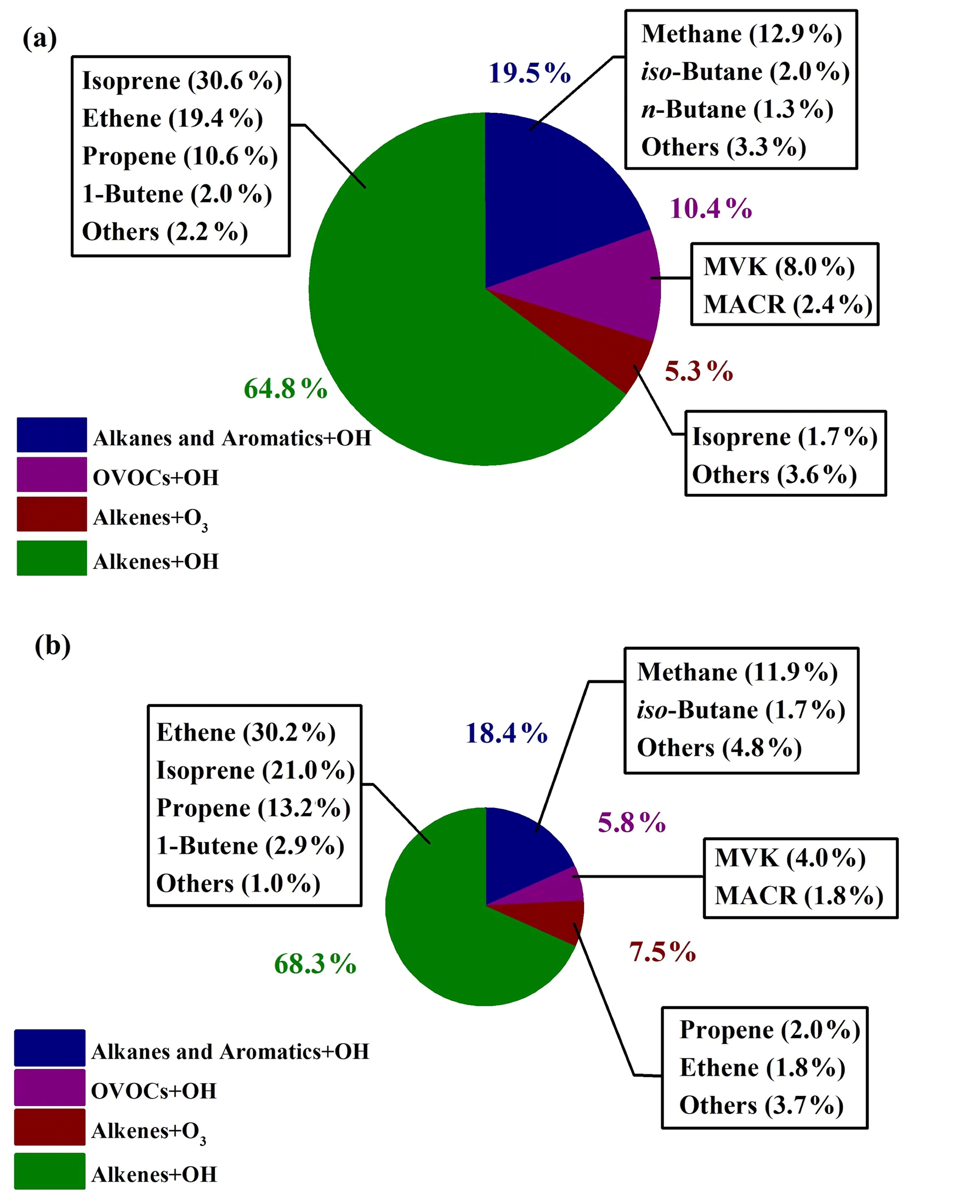
Figure 7Relative contributions to HCHO production rates in (a) the sunny period and (b) the cloudy and rainy period. The relative contributions to HCHO production are shown for the top 10 VOC species in each period. The area of pie charts is in proportion to the calculated HCHO production rates in two periods.
For the cloudy and rainy period (Fig. 7b), the relative contribution to secondary HCHO from OH-radical-initiated reactions with alkenes increased a little, accounting for 68.3 %, while OVOCs oxidation by OH radicals decreased to 5.8 %. MVK and MACR are known as the major intermediate products generated from isoprene oxidation. The less intensive solar radiation on the cloudy and rainy days influences both the abundance and the oxidation processes of MVK and MACR to form HCHO, leading to their declined fraction of HCHO production (Gong et al., 2018; Guo et al., 2012; Gu et al., 2022). Meanwhile, the total contribution from isoprene oxidation decreased to 21.0 % due to the combination of lower isoprene concentrations and OH abundances. On the cloudy and rainy days, the dominant pathways to HCHO production were OH-radical-initiated reactions with ethene, isoprene, propene, and methane, yielding 30.2 %, 21.0 %, 13.2 %, and 11.9 %, respectively, of the total HCHO production from VOCs we have measured.
For both the sunny period and the cloudy and rainy period, ethene and propene turned out to be two of the most important precursors, but their significance has not been reported in previous studies, which might be attributed to the forest environments where most previous studies were conducted (Choi et al., 2010; Sumner et al., 2001). Also, the importance of MVK and MACR was not found previously, but these two precursors turned out to play an important role in secondary HCHO production in our study. To the best of our knowledge, there is only one study that has previously calculated HCHO production from various alkanes in an urban area in the USA (Lin et al., 2012). Our study takes a wide range of VOCs including alkanes, alkenes, aromatic, and OVOCs into account in the calculation of HCHO production rates.
The average diurnal patterns of secondary HCHO production showed clear differences between the sunny and the cloudy and rainy periods, as shown in Fig. 8. During the sunny period (Fig. 8a), HCHO production rates displayed a strong diurnal cycle, with a peak of 3.80 ppbv h−1 observed at 13:00 LT, when photochemical reactions were intense, and were roughly constant at about 0.03 ppbv h−1 during nighttime (from 19:00 to 05:00 LT the next day). During this low-rate period, about 98 % of the HCHO production came from ozonolysis of alkenes, since the estimated average nighttime concentration of OH radicals was lower than 1500 molec. cm−3, i.e., 5.58 × 10⁻⁵ pptv, while that of O3 was still as high as 5.68 × 10¹¹ molec. cm−3, i.e., 21.15 ppbv. After sunrise at 05:00 LT, HCHO production rates increased dramatically, reaching a maximum of 3.80 ppbv h−1 at 13:00 LT, and then reduced until sunset at around 18:00 LT. Although O3 concentration was higher than that of OH radicals during the daytime, the rate constants for reactions of alkenes with O3 are several orders of magnitude lower than those with OH, resulting in the dominant HCHO formation by alkene oxidation with OH.
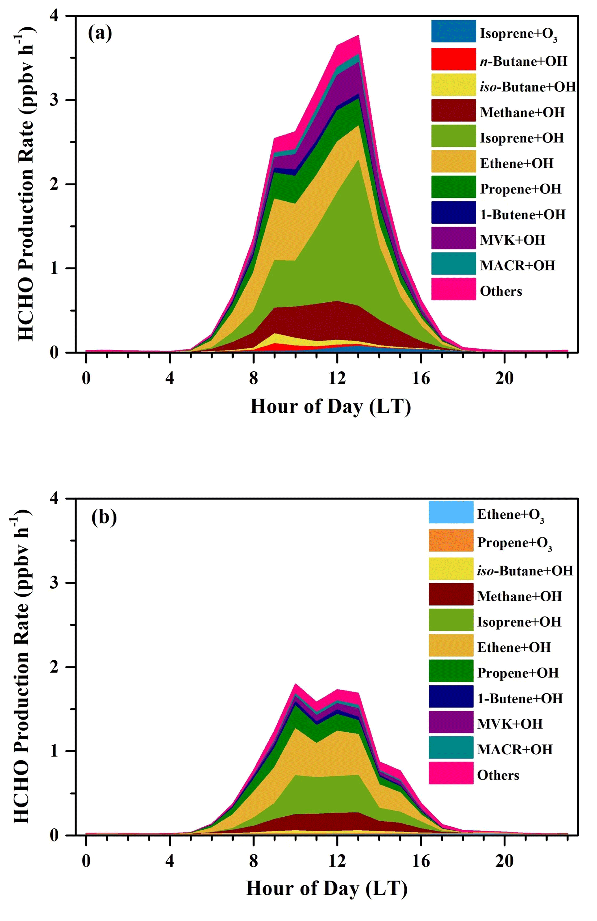
Figure 8Average diurnal variations in HCHO production rates (ppbv h−1) from the OH-initiated and O3-initiated oxidation during (a) the sunny period and (b) the cloudy and rainy period.
In the cloudy and rainy period (Fig. 8b), nighttime HCHO production rates were almost equivalent to those on the sunny days and also dominantly came from alkene ozonolysis. Secondary HCHO production rates began to rise after 05:00 LT, peaked at 10:00 LT (1.82 ppbv h−1), remained high (∼ 1.69 ppbv h−1) until 13:00 LT, and then started to fall to low values at night. This trend is consistent with the variation in the photolysis frequencies, which maintained the highest values between 10:00–13:00 LT on the rainy and cloudy days, whereas they kept growing after sunrise and peaked at 13:00 LT on the sunny days. The 24 h average HCHO production rates on the cloudy and rainy days (0.51 ppbv h−1) were nearly half of the average on the sunny days (0.97 ppbv h−1).
By applying the root square propagation of uncertainties in the reaction rate coefficients and corresponding HCHO yields for reactions between VOCs and oxidants, measurements of 24 VOCs and ozone, and estimations of OH (Table S6), the total uncertainties in the HCHO production rates were estimated to be 25.9 % in the sunny period and 21.0 % in the cloudy and rainy period.
3.3 HCHO sinks
Reactions (R1)–(R3) show the dominant daytime chemical loss processes of HCHO, i.e, direct oxidation by OH radicals, and two different photolysis pathways. The overall HCHO loss rate by photolysis can be calculated from measured HCHO concentration and its photolysis rate constants, J(HCHO_M) and J(HCHO_R) (shown in Table S1). These major daytime sinks of HCHO ultimately produce hydroperoxy (HO2) radicals. As reported in previous studies, HCHO represents an important source of HO2 radicals in the atmosphere (Mahajan et al., 2010; Tan et al., 2019a, b).
Compared with daytime, photolysis frequencies and OH radical concentrations at night are really low so that oxidation of HCHO by OH radicals and photolysis are ineffective sinks. Instead, HCHO dry deposition become the most important nocturnal removal process at night; it depends on both its loss at the surface (described by a surface resistance) and transport to the surface (Fischer et al., 2019; Nussbaumer et al., 2021; Choi et al., 2010; Nguyen et al., 2015; Sumner et al., 2001; Anderson et al., 2017). The HCHO deposition velocity vd can be estimated from its nighttime concentration decrease (Nussbaumer et al., 2021; Fischer et al., 2019). An average loss rate constant kd was determined from the HCHO concentration decline from 21:00–01:00 LT divided by the average HCHO concentration during this time interval according to Eq. (7).
Then the HCHO deposition velocity could be calculated by Eq. (8).
where BLH denotes the boundary layer height. To consider the inconsistent mixing of the boundary layer at night, the factor x is equal to 2, assuming a linear increase in the HCHO mixing ratio with height in the nocturnal boundary layer (Shepson et al., 1992). During the day, x is set to be 1 for a boundary layer that is well mixed (Fischer et al., 2019; Nussbaumer et al., 2021). Note that this estimation of the dry-deposition loss is a lower limit, since it neglects nighttime production of HCHO due to ozonolysis of alkenes, as well as thermally driven turbulence and deposition caused by stomatal uptake by vegetation (Fischer et al., 2019; Nguyen et al., 2015). Figure S4 shows an example of one of the evenings during which HCHO decay followed apparent first-order kinetics. We have performed this calculation for nine nights when the estimated HCHO production from ozonolysis of alkenes was around 15 % of the observed HCHO loss on average, and an overview of the nine nights can be found in Fig. S5. We finally estimated vd (night) = 0.52 cm s−1 and vd (day) = 1.04 cm s−1. Table 2 compares dry-deposition rates of HCHO reported in previous studies to our estimates, which turn out to be quite similar (DiGangi et al., 2011; Ayers et al., 1997; Stickler et al., 2007; Nussbaumer et al., 2021; Sumner et al., 2001; Choi et al., 2010).

By our estimation, the role of NO3 radicals in HCHO removal at the DSL site was negligible (Sect. S3). Therefore, calculation of the HCHO loss could be expressed as in Eq. (9).
The profile of the calculated HCHO loss rates during the campaign is shown in Fig. S6, with an average loss rate of 0.49 ppbv h−1. Comparison of HCHO loss rates between the sunny period and the cloudy and rainy period is shown in Table 1.
In Fig. 9, the average diurnal HCHO loss rates in both the sunny period and the cloudy and rainy period showed significant diurnal cycles. Daily average loss rates of dry deposition did not show an obvious diurnal cycle and remained relatively constant, ranging from 0.08 to 0.40 ppbv h−1 in the sunny period and 0.04 to 0.12 ppbv h−1 in the cloudy and rainy period, owing to covariation in the concentration of HCHO and BLH. During nighttime in both periods, HCHO loss rates were dominated by dry deposition, when the contributions of photolysis and reactions with OH were so small that they could be neglected. After sunrise, loss rates of photolysis and the reaction with OH radicals began to rise and reached the maximum at noon. The diurnal maximum loss rate in the sunny period was 2.75 ppbv h−1, about 3 times larger than that in the cloudy and rainy period (0.66 ppbv h−1), both of which occurred at 13:00 LT. After the peak, loss rates of photolysis and the reaction with OH in both periods continued to fall and remained low at night. The 24 h average loss rates of HCHO were 0.78 and 0.22 ppbv h−1 for the sunny period and the cloudy and rainy period, respectively. Dry deposition played a more important role in HCHO loss in the cloudy and rainy period, accounting for 34.1 % of the loss of HCHO, whereas photolysis contributed 32.8 %, and the reaction with OH radicals contributed 33.1 %. Reaction with OH radicals was the dominant contributor to HCHO loss in the sunny period, which represented 42.2 % of the total HCHO loss, followed by photolysis (39.2 %) and dry deposition (18.6 %).
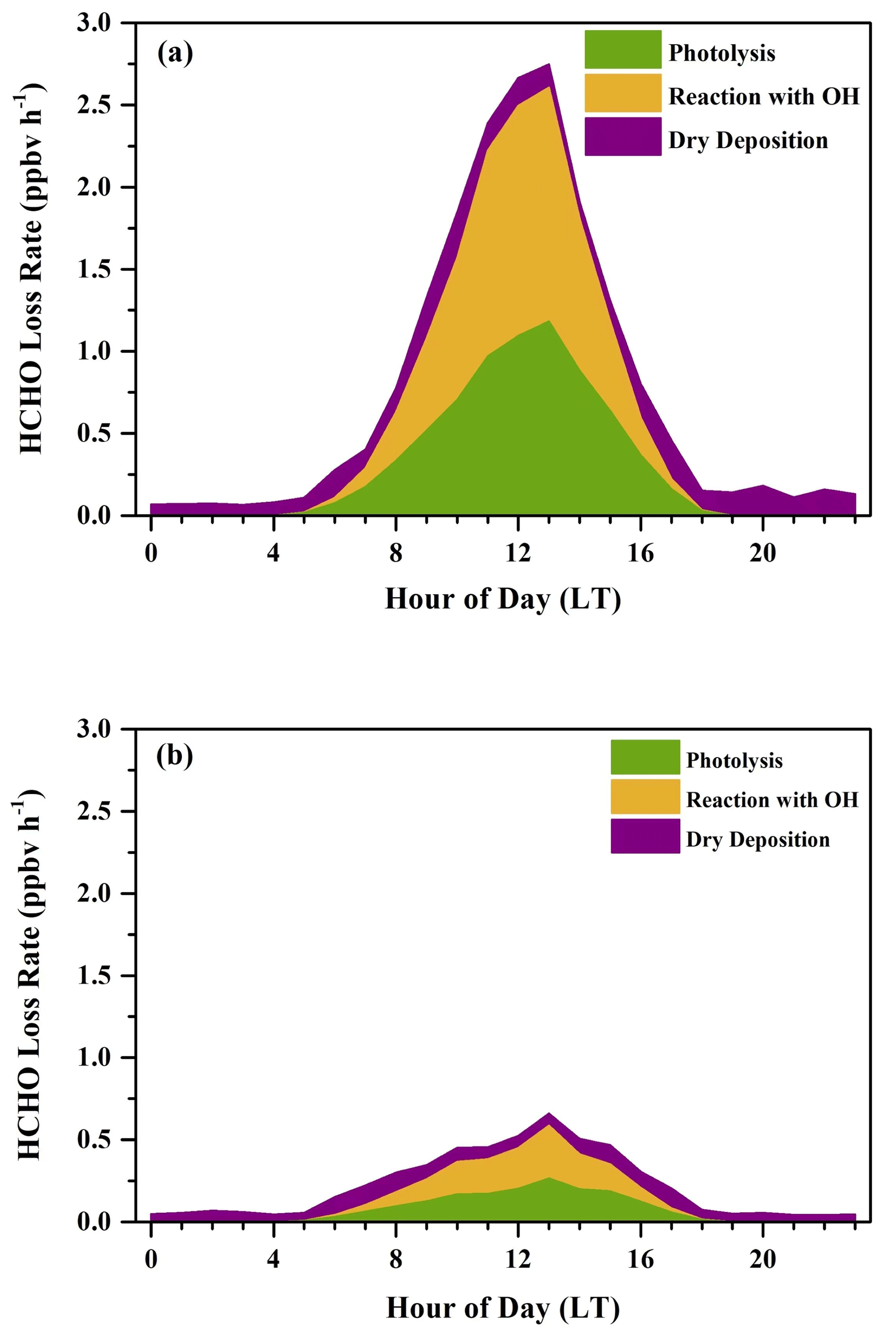
Figure 9Average diurnal variations in HCHO loss rates (ppbv h−1) determined from photolysis, reaction with OH radicals, and dry deposition during (a) the sunny period and (b) the cloudy and rainy period.
The total uncertainties in HCHO loss rates resulted from the uncertainties in the reaction rate coefficients for VOCs and OH radicals, measurements of HCHO, photolysis frequencies, and BLH, and estimations of OH (Table S7) were 28.9 % in both the sunny period and the cloudy and rainy period.
3.4 HCHO net production
We investigated the daily profiles of hourly averages of HCHO production and loss rates throughout the campaign. Net production of HCHO can be calculated as in Eq. (10).
Uncertainties in the calculated net HCHO production rates and the observed rates of HCHO concentration change are listed in Table S8. The uncertainty in the observed rates of HCHO concentration change is composed of the HCHO measurement uncertainty and the uncertainty in the fit (30 % upper limit) (Nussbaumer et al., 2021), with the latter dominating. Any discrepancy between the calculated net HCHO production rates and the observed rates of HCHO concentration change will be due to either unconsidered chemical terms or meteorological effects (Sumner et al., 2001). Figure 10a shows that our calculated net HCHO production rates are in relatively good agreement with the observed rates of HCHO concentration change throughout the day in the sunny period, indicating that our treatment of chemical terms is accurate and that HCHO was dominantly secondarily produced at the DSL site, which can be approximated by oxidation of the 24 hydrocarbons we considered in our calculation. Thus, transport processes and primary emissions did not significantly impact ambient HCHO concentrations at the DSL site; at least their influences were considerably tiny compared to the chemical production. During nighttime, the rates of HCHO concentration change oscillated around zero, when the calculated production almost completely balanced the loss term. After 07:00 LT, HCHO production exceeded its loss, leading to positive net HCHO production values, which is in line with the increasing trend of the HCHO concentration. After 15:00 LT, HCHO loss began to transcend its production, resulting in the decline in HCHO abundance. Uncertainties in the calculated net HCHO production rates (38.8 %) and the observed rates of HCHO concentration change (30 %) led to overlapped uncertainty ranges, as shown in Fig. 10a. Thus, the calculated net HCHO production rates are very close to the observed rates of HCHO concentration change. However, during 12:00–14:00 LT, the calculated net HCHO production rates were slightly higher than the observed rates of HCHO concentration change by around 0.6 ppbv h−1, indicating a missing loss term, most likely due to dilution with HCHO-poor air from the nocturnal residual layer, which coincided with the obvious enhancements of the boundary layer height that were usually observed during 11:00–14:00 LT at the DSL site, as shown in Fig. S7a.
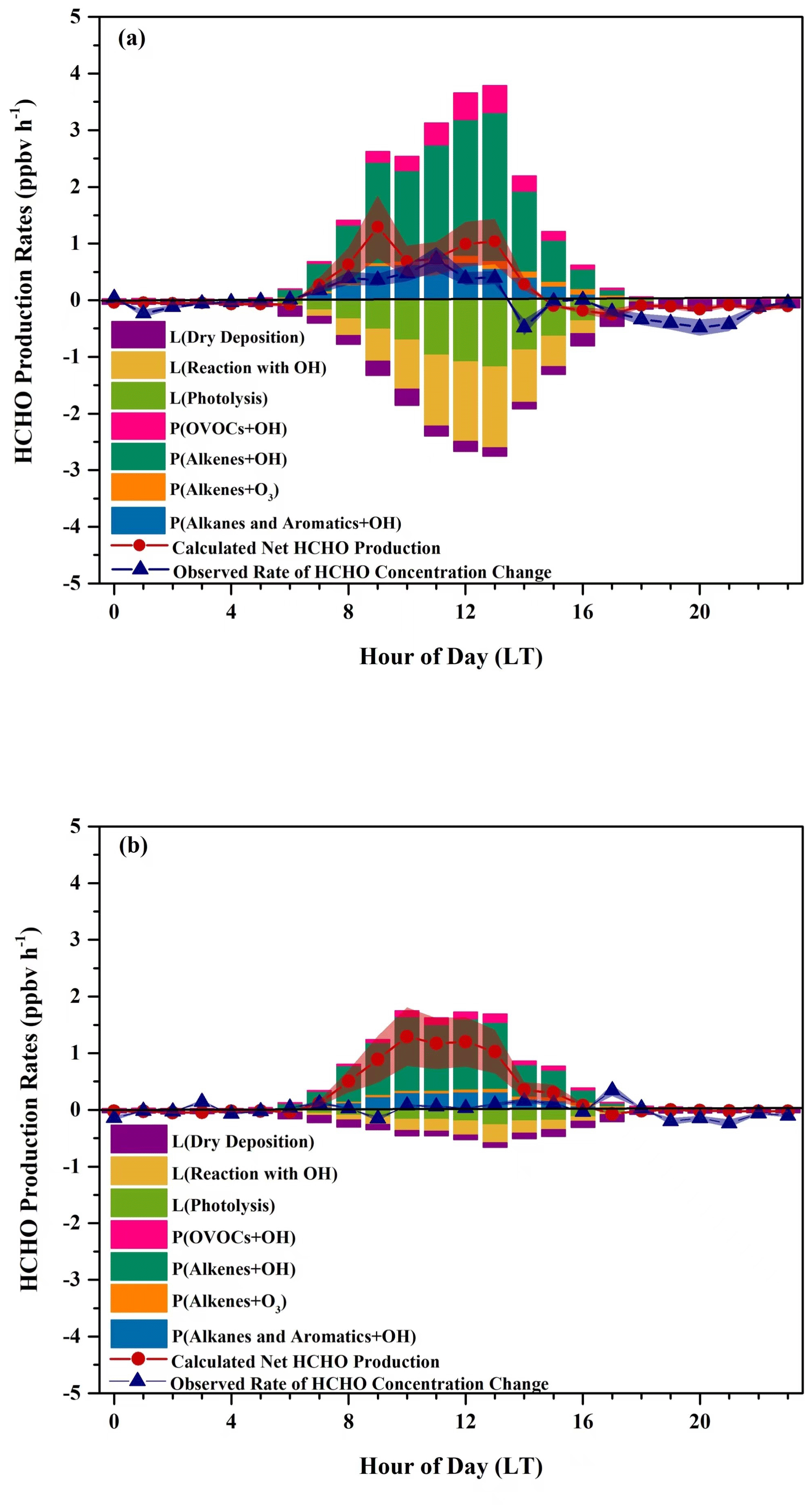
Figure 10Average diurnal variations in HCHO production rates, HCHO loss rates, the calculated net production rates, and the observed rates of HCHO concentration change during (a) the sunny and (b) the cloudy and rainy period. Shaded areas give the uncertainties in the calculated net production rates and the observed rates of HCHO concentration change.
On the other hand, on the cloudy and rainy days, the observed HCHO concentration remained relatively steady, while calculated HCHO production prevailed over its loss, leading to a net production of about 1 ppbv h−1 during 08:00–13:00 LT, as shown in Fig. 10b. The differences between the calculated net production rates and the observed rates of HCHO concentration change suggest either a missing loss term or an overestimated production. Since differences were still observed from 08:00–13:00 LT in Fig. 10b even when uncertainties in the calculated net HCHO production rates (35.7 %) and the observed rates of HCHO concentration change (30 %) were considered, a real missing loss term was more likely there. Dilution with HCHO-poor air from the nocturnal residual layer due to the increases in the boundary layer height, as we discuss for the case in the sunny period, might have contributed to the missing loss term but probably was not the only donor since the discrepancies found between 12:00–14:00 LT on the sunny days were only half of those found on the cloudy and rainy days, whereas the increases in the boundary layer height on the cloudy and rainy days were smaller compared to those on the sunny days, as shown in Fig. S7b. Also, the wind speeds were usually between 1–3 m s−1, which indicates that transport effects from areas with lower HCHO concentrations might not be important. There was significantly more rainfall at daytime on the cloudy and rainy days than on the sunny days during our campaign, and thus we assume the other missing loss process might be wet deposition, which has been reported as a dominant process in the total deposition (i.e., dry deposition and wet deposition) during the rainy season (Seyfioglu et al., 2006). Indeed, HCHO is readily soluble in cloud and rainwater with its high Henry's law constant (∼ 5.5 × 10³ M atm−1) and could be efficiently converted to formic acid in warm cloud droplets (Allou et al., 2011; Chebbi and Carlier, 1996; Franco et al., 2021). Unfortunately, we did not collect rain samples during our campaign so that we are unable to further evaluate this assumption.
In this study, ambient HCHO measurements, together with a number of VOC species, were conducted from 10 June to 4 July in 2021 at the DSL site in Shanghai. During the campaign, the average HCHO concentration was 2.2 ± 1.8 ppbv. The good correlation of HCHO and O3 (R2 = 0.73) and the two methods of estimating the contributions of different HCHO sources (i.e., HCHO C2H2 ratios and a multi-linear regression method based on ambient measurements of HCHO, C2H2, and O3) both indicate that secondary sources played an important role in the local HCHO formation. A total of 24 VOC species were considered in the calculation of secondary HCHO production, which shows that the dominant HCHO precursors were isoprene, ethene, methane, and propene. In the sunny period, isoprene oxidation by OH radicals contributed the most, whereas reactions of ethene with OH radicals became the most important path to the HCHO production in the cloudy and rainy period. The 24 h average secondary HCHO production rates were 0.97 and 0.51 ppbv h−1 for the sunny period and the cloudy and rainy period, respectively. For the HCHO loss estimation, HCHO photolysis, reactions with OH radicals, and dry deposition were considered, where loss rates due to photolysis and reactions of OH radicals were significantly larger than those of dry deposition in the sunny period, but these three terms were nearly equivalent in the cloudy and rainy period. The 24 h average loss rates of HCHO were 0.78 and 0.22 ppbv h−1 for the sunny period and the cloudy and rainy period, respectively. The calculated net HCHO production rates were in good agreement with the observed rates of HCHO concentration change throughout the sunny days, indicating that HCHO was approximately produced by oxidation of the 24 VOC species we considered at the DSL site during the campaign.
In summary, our results reveal the important role of secondary formation of HCHO in the suburbs of Shanghai, where alkenes are likely the key precursors for HCHO. We provide a HCHO budget based on a comprehensive observation of HCHO precursors, which has rarely been conducted in previous studies. Meanwhile, we found evidence for missing loss processes of HCHO on the cloudy and rainy days, which might be attributed to the HCHO wet deposition, and this may be an important loss term on rainy days and should be further investigated.
The data used to support the conclusions in this study are available at a public data repository of Figshare via https://doi.org/10.6084/m9.figshare.20218133.v3 (Wu, 2022).
The supplement related to this article is available online at: https://doi.org/10.5194/acp-23-2997-2023-supplement.
LinW designed the study. YiW, JH, GY, YuW, SW, and QF conducted the field campaign. YiW, GY, YuW, and LihW carried out laboratory experiments. JH, SW, QF, and LY provided technical support. YiW analyzed the data. YiW and LinW wrote the paper with contributions from all of the other co-authors.
The contact author has declared that none of the authors has any competing interests.
Publisher’s note: Copernicus Publications remains neutral with regard to jurisdictional claims in published maps and institutional affiliations.
This research has been supported by the National Natural Science Foundation of China (grant nos. 21925601, 92044301, 92143301, and 22127811) and the Shanghai Municipal Bureau of Ecology and Environment (grant no. 2021-29).
This paper was edited by Andreas Hofzumahaus and reviewed by two anonymous referees.
Allou, L., El Maimouni, L., and Le Calvé, S.: Henry's law constant measurements for formaldehyde and benzaldehyde as a function of temperature and water composition, Atmos. Environ., 45, 2991–2998, https://doi.org/10.1016/j.atmosenv.2010.05.044, 2011.
Anderson, D. C., Nicely, J. M., Wolfe, G. M., Hanisco, T. F., Salawitch, R. J., Canty, T. P., Dickerson, R. R., Apel, E. C., Baidar, S., Bannan, T. J., Blake, N. J., Chen, D., Dix, B., Fernandez, R. P., Hall, S. R., Hornbrook, R. S., Gregory Huey, L., Josse, B., Jöckel, P., Kinnison, D. E., Koenig, T. K., Le Breton, M., Marécal, V., Morgenstern, O., Oman, L. D., Pan, L. L., Percival, C., Plummer, D., Revell, L. E., Rozanov, E., Saiz-Lopez, A., Stenke, A., Sudo, K., Tilmes, S., Ullmann, K., Volkamer, R., Weinheimer, A. J., Zeng, G., Huey, L. G., Josse, B., Joeckel, P., Kinnison, D. E., Koenig, T. K., Le Breton, M., Marecal, V., Morgenstern, O., Oman, L. D., Pan, L. L., Percival, C., Plummer, D., Revell, L. E., Rozanov, E., Saiz-Lopez, A., Stenke, A., Sudo, K., Tilmes, S., Ullmann, K., Volkamer, R., Weinheimer, A. J., and Zeng, G.: Formaldehyde in the Tropical Western Pacific: Chemical Sources and Sinks, Convective Transport, and Representation in CAM-Chem and the CCMI Models, J. Geophys. Res.-Atmos., 122, 11201–11226, https://doi.org/10.1002/2016JD026121, 2017.
Ayers, G. P., Gillett, R. W., Granek, H., De Serves, C., and Cox, R. A.: Formaldehyde production in clean marine air, Geophys. Res. Lett., 24, 401–404, https://doi.org/10.1029/97GL00123, 1997.
Chebbi, A. and Carlier, P.: Carboxylic acids in the troposphere, occurrence, sources, and sinks: A review, Atmos. Environ., 30, 4233–4249, https://doi.org/10.1016/1352-2310(96)00102-1, 1996.
Chen, W. T., Shao, M., Lu, S. H., Wang, M., Zeng, L. M., Yuan, B., and Liu, Y.: Understanding primary and secondary sources of ambient carbonyl compounds in Beijing using the PMF model, Atmos. Chem. Phys., 14, 3047–3062, https://doi.org/10.5194/acp-14-3047-2014, 2014.
Choi, W., Faloona, I. C., Bouvier-Brown, N. C., McKay, M., Goldstein, A. H., Mao, J., Brune, W. H., LaFranchi, B. W., Cohen, R. C., Wolfe, G. M., Thornton, J. A., Sonnenfroh, D. M., and Millet, D. B.: Observations of elevated formaldehyde over a forest canopy suggest missing sources from rapid oxidation of arboreal hydrocarbons, Atmos. Chem. Phys., 10, 8761–8781, https://doi.org/10.5194/acp-10-8761-2010, 2010.
Claflin, M. S., Pagonis, D., Finewax, Z., Handschy, A. V., Day, D. A., Brown, W. L., Jayne, J. T., Worsnop, D. R., Jimenez, J. L., Ziemann, P. J., de Gouw, J., and Lerner, B. M.: An in situ gas chromatograph with automatic detector switching between PTR- and EI-TOF-MS: isomer-resolved measurements of indoor air, Atmos. Meas. Tech., 14, 133–152, https://doi.org/10.5194/amt-14-133-2021, 2021.
de Gouw, J. A., Middlebrook, A. M., Warneke, C., Goldan, P. D., Kuster, W. C., Roberts, J. M., Fehsenfeld, F. C., Worsnop, D. R., Canagaratna, M. R., Pszenny, A. A. P., Keene, W. C., Marchewka, M., Bertman, S. B., and Bates, T. S.: Budget of organic carbon in a polluted atmosphere: Results from the New England Air Quality Study in 2002, J. Geophys. Res.-Atmos., 110, 1–22, https://doi.org/10.1029/2004JD005623, 2005.
de Gouw, J. A., Gilman, J. B., Kim, S. W., Alvarez, S. L., Dusanter, S., Graus, M., Griffith, S. M., Isaacman-VanWertz, G., Kuster, W. C., Lefer, B. L., Lerner, B. M., McDonald, B. C., Rappenglück, B., Roberts, J. M., Stevens, P. S., Stutz, J., Thalman, R., Veres, P. R., Volkamer, R., Warneke, C., Washenfelder, R. A., and Young, C. J.: Chemistry of Volatile Organic Compounds in the Los Angeles Basin: Formation of Oxygenated Compounds and Determination of Emission Ratios, J. Geophys. Res.-Atmos., 123, 2298–2319, https://doi.org/10.1002/2017JD027976, 2018.
DiGangi, J. P., Boyle, E. S., Karl, T., Harley, P., Turnipseed, A., Kim, S., Cantrell, C., Maudlin III, R. L., Zheng, W., Flocke, F., Hall, S. R., Ullmann, K., Nakashima, Y., Paul, J. B., Wolfe, G. M., Desai, A. R., Kajii, Y., Guenther, A., and Keutsch, F. N.: First direct measurements of formaldehyde flux via eddy covariance: implications for missing in-canopy formaldehyde sources, Atmos. Chem. Phys., 11, 10565–10578, https://doi.org/10.5194/acp-11-10565-2011, 2011.
Dovrou, E., Bates, K. H., Moch, J. M., Mickley, L. J., Jacob, D. J., and Keutsch, F. N.: Catalytic role of formaldehyde in particulate matter formation, P. Natl. Acad. Sci. USA, 119, e2113265119, https://doi.org/10.1073/pnas.2113265119, 2022.
Dutta, C., Chatterjee, A., Jana, T. K., Mukherjee, A. K., and Sen, S.: Contribution from the primary and secondary sources to the atmospheric formaldehyde in Kolkata, India, Sci. Total Environ., 408, 4744–4748, https://doi.org/10.1016/j.scitotenv.2010.01.031, 2010.
Ehhalt, D. H. and Rohrer, F.: Dependence of the OH concentration on solar UV, J. Geophys. Res.-Atmos., 105, 3565–3571, https://doi.org/10.1029/1999JD901070, 2000.
Fan, X., Cai, J., Yan, C., Zhao, J., Guo, Y., Li, C., Dällenbach, K. R., Zheng, F., Lin, Z., Chu, B., Wang, Y., Dada, L., Zha, Q., Du, W., Kontkanen, J., Kurtén, T., Iyer, S., Kujansuu, J. T., Petäjä, T., Worsnop, D. R., Kerminen, V.-M., Liu, Y., Bianchi, F., Tham, Y. J., Yao, L., and Kulmala, M.: Atmospheric gaseous hydrochloric and hydrobromic acid in urban Beijing, China: detection, source identification and potential atmospheric impacts, Atmos. Chem. Phys., 21, 11437–11452, https://doi.org/10.5194/acp-21-11437-2021, 2021.
Fischer, H., Axinte, R., Bozem, H., Crowley, J. N., Ernest, C., Gilge, S., Hafermann, S., Harder, H., Hens, K., Janssen, R. H. H., Königstedt, R., Kubistin, D., Mallik, C., Martinez, M., Novelli, A., Parchatka, U., Plass-Dülmer, C., Pozzer, A., Regelin, E., Reiffs, A., Schmidt, T., Schuladen, J., and Lelieveld, J.: Diurnal variability, photochemical production and loss processes of hydrogen peroxide in the boundary layer over Europe, Atmos. Chem. Phys., 19, 11953–11968, https://doi.org/10.5194/acp-19-11953-2019, 2019.
Franco, B., Blumenstock, T., Cho, C., Clarisse, L., Clerbaux, C., Coheur, P. F., De Mazière, M., De Smedt, I., Dorn, H. P., Emmerichs, T., Fuchs, H., Gkatzelis, G., Griffith, D. W. T., Gromov, S., Hannigan, J. W., Hase, F., Hohaus, T., Jones, N., Kerkweg, A., Kiendler-Scharr, A., Lutsch, E., Mahieu, E., Novelli, A., Ortega, I., Paton-Walsh, C., Pommier, M., Pozzer, A., Reimer, D., Rosanka, S., Sander, R., Schneider, M., Strong, K., Tillmann, R., Van Roozendael, M., Vereecken, L., Vigouroux, C., Wahner, A., and Taraborrelli, D.: Ubiquitous atmospheric production of organic acids mediated by cloud droplets, Nature, 593, 233–237, https://doi.org/10.1038/s41586-021-03462-x, 2021.
Garcia, A. R., Volkamer, R., Molina, L. T., Molina, M. J., Samuelson, J., Mellqvist, J., Galle, B., Herndon, S. C., and Kolb, C. E.: Separation of emitted and photochemical formaldehyde in Mexico City using a statistical analysis and a new pair of gas-phase tracers, Atmos. Chem. Phys., 6, 4545–4557, https://doi.org/10.5194/acp-6-4545-2006, 2006.
Gong, D., Wang, H., Zhang, S., Wang, Y., Liu, S. C., Guo, H., Shao, M., He, C., Chen, D., He, L., Zhou, L., Morawska, L., Zhang, Y., and Wang, B.: Low-level summertime isoprene observed at a forested mountaintop site in southern China: implications for strong regional atmospheric oxidative capacity, Atmos. Chem. Phys., 18, 14417–14432, https://doi.org/10.5194/acp-18-14417-2018, 2018.
Gu, C., Wang, S., Zhu, J., Wu, S., Duan, Y., Gao, S., and Zhou, B.: Investigation on the urban ambient isoprene and its oxidation processes, Atmos. Environ., 270, 118870, https://doi.org/10.1016/j.atmosenv.2021.118870, 2022.
Guo, H., Ling, Z. H., Simpson, I. J., Blake, D. R., and Wang, D. W.: Observations of isoprene, methacrolein (MAC) and methyl vinyl ketone (MVK) at a mountain site in Hong Kong, J. Geophys. Res.-Atmos., 117, 1–13, https://doi.org/10.1029/2012JD017750, 2012.
Han, Y., Huang, X., Wang, C., Zhu, B., and He, L.: Characterizing oxygenated volatile organic compounds and their sources in rural atmospheres in China, J. Environ. Sci. (China), 81, 148–155, https://doi.org/10.1016/j.jes.2019.01.017, 2019.
Helmig, D.: Ozone removal techniques in the sampling of atmospheric volatile organic trace gases, Atmos. Environ., 31, 3635–3651, https://doi.org/10.1016/S1352-2310(97)00144-1, 1997.
Ho, K. F., Ho, S. S. H., Huang, R. J., Dai, W. T., Cao, J. J., Tian, L., and Deng, W. J.: Spatiotemporal distribution of carbonyl compounds in China, Environ. Pollut., 197, 316–324, https://doi.org/10.1016/j.envpol.2014.11.014, 2015.
Hong, Q., Zhu, L., Xing, C., Hu, Q., Lin, H., Zhang, C., Zhao, C., Liu, T., Su, W., and Liu, C.: Inferring vertical variability and diurnal evolution of O3 formation sensitivity based on the vertical distribution of summertime HCHO and NO2 in Guangzhou, China., Sci. Total Environ., 827, 154045, https://doi.org/10.1016/j.scitotenv.2022.154045, 2022.
Kumar, V. and Sinha, V.: VOC–OHM: A new technique for rapid measurements of ambient total OH reactivity and volatile organic compounds using a single proton transfer reaction mass spectrometer, Int. J. Mass Spectrom., 374, 55–63, https://doi.org/10.1016/j.ijms.2014.10.012, 2014.
Lee, Y. N., Zhou, X., Kleinman, L. I., Nunnermacker, L. J., Springston, S. R., Daum, P. H., Newman, L., Keigley, W. G., Holdren, M. W., Spicer, C. W., Young, V., Fu, B., Parrish, D. D., Holloway, J., Williams, J., Roberts, J. M., Ryerson, T. B., and Fehsenfeld, F. C.: Atmospheric chemistry and distribution of formaldehyde and several multioxygenated carbonyl compounds during the 1995 Nashville/Middle Tennessee Ozone Study, J. Geophys. Res.-Atmos., 103, 22449–22462, https://doi.org/10.1029/98JD01251, 1998.
Li, J., Xie, S. D., Zeng, L. M., Li, L. Y., Li, Y. Q., and Wu, R. R.: Characterization of ambient volatile organic compounds and their sources in Beijing, before, during, and after Asia-Pacific Economic Cooperation China 2014, Atmos. Chem. Phys., 15, 7945–7959, https://doi.org/10.5194/acp-15-7945-2015, 2015.
Lin, Y. C., Schwab, J. J., Demerjian, K. L., Bae, M.-S. S., Chen, W.-N. N., Sun, Y., Zhang, Q., Hung, H.-M. M., and Perry, J.: Summertime formaldehyde observations in New York City: Ambient levels, sources and its contribution to HOx radicals, J. Geophys. Res.-Atmos., 117, 1–14, https://doi.org/10.1029/2011JD016504, 2012.
Liu, L., Flatøy, F., Ordóñez, C., Braathen, G. O., Hak, C., Junkermann, W., Andreani-Aksoyoglu, S., Mellqvist, J., Galle, B., Prévôt, A. S. H., and Isaksen, I. S. A.: Photochemical modelling in the Po basin with focus on formaldehyde and ozone, Atmos. Chem. Phys., 7, 121–137, https://doi.org/10.5194/acp-7-121-2007, 2007.
Liu, Y., Zhang, Y., Lian, C., Yan, C., Feng, Z., Zheng, F., Fan, X., Chen, Y., Wang, W., Chu, B., Wang, Y., Cai, J., Du, W., Daellenbach, K. R., Kangasluoma, J., Bianchi, F., Kujansuu, J., Petäjä, T., Wang, X., Hu, B., Wang, Y., Ge, M., He, H., and Kulmala, M.: The promotion effect of nitrous acid on aerosol formation in wintertime in Beijing: the possible contribution of traffic-related emissions, Atmos. Chem. Phys., 20, 13023–13040, https://doi.org/10.5194/acp-20-13023-2020, 2020.
Mahajan, A. S., Whalley, L. K., Kozlova, E., Oetjen, H., Mendez, L., Furneaux, K. L., Goddard, A., Heard, D. E., Plane, J. M. C., and Saiz-Lopez, A.: DOAS observations of formaldehyde and its impact on the HOx balance in the tropical Atlantic marine boundary layer, J. Atmos. Chem., 66, 167–178, https://doi.org/10.1007/s10874-011-9200-7, 2010.
Nguyen, T. B., Crounse, J. D., Teng, A. P., Clair, J. M. S., Paulot, F., Wolfe, G. M., and Wennberg, P. O.: Rapid deposition of oxidized biogenic compounds to a temperate forest, P. Natl. Acad. Sci. USA, 112, E392–E401, https://doi.org/10.1073/pnas.1418702112, 2015.
Nussbaumer, C. M., Crowley, J. N., Schuladen, J., Williams, J., Hafermann, S., Reiffs, A., Axinte, R., Harder, H., Ernest, C., Novelli, A., Sala, K., Martinez, M., Mallik, C., Tomsche, L., Plass-Dülmer, C., Bohn, B., Lelieveld, J., and Fischer, H.: Measurement report: Photochemical production and loss rates of formaldehyde and ozone across Europe, Atmos. Chem. Phys., 21, 18413–18432, https://doi.org/10.5194/acp-21-18413-2021, 2021.
Obersteiner, F., Bönisch, H., and Engel, A.: An automated gas chromatography time-of-flight mass spectrometry instrument for the quantitative analysis of halocarbons in air, Atmos. Meas. Tech., 9, 179–194, https://doi.org/10.5194/amt-9-179-2016, 2016.
Pavel, M. R. S., Zaman, S. U., Jeba, F., and Salam, A.: Long-Term (2011–2019) Trends of O3, NO2, and HCHO and Sensitivity Analysis of O3 Chemistry over the GBM (Ganges-Brahmaputra-Meghna) Delta: Spatial and Temporal Variabilities, ACS Earth Sp. Chem., 5, 1468–1485, https://doi.org/10.1021/acsearthspacechem.1c00057, 2021.
Possanzini, M., Di Palo, V., and Cecinato, A.: Sources and photodecomposition of formaldehyde and acetaldehyde in Rome ambient air, Atmos. Environ., 36, 3195–3201, https://doi.org/10.1016/S1352-2310(02)00192-9, 2002.
Rohrer, F. and Berresheim, H.: Strong correlation between levels of tropospheric hydroxyl radicals and solar ultraviolet radiation, Nature, 442, 184–187, https://doi.org/10.1038/nature04924, 2006.
Seyfioglu, R., Odabasi, M., and Cetin, E.: Wet and dry deposition of formaldehyde in Izmir, Turkey, Sci. Total Environ., 366, 809–818, https://doi.org/10.1016/j.scitotenv.2005.08.005, 2006.
Shepson, P. B., Bottenheim, J. W., and Hastie, D. R.: Determination of the relative ozone and PAN deposition velocities at night, Geophys. Res. Lett., 19, 1121–1124, 1992.
Stickler, A., Fischer, H., Bozem, H., Gurk, C., Schiller, C., Martinez-Harder, M., Kubistin, D., Harder, H., Williams, J., Eerdekens, G., Yassaa, N., Ganzeveld, L., Sander, R., and Lelieveld, J.: Chemistry, transport and dry deposition of trace gases in the boundary layer over the tropical Atlantic Ocean and the Guyanas during the GABRIEL field campaign, Atmos. Chem. Phys., 7, 3933–3956, https://doi.org/10.5194/acp-7-3933-2007, 2007.
Su, W., Liu, C., Hu, Q., Zhao, S., Sun, Y., Wang, W., Zhu, Y., Liu, J., and Kim, J.: Primary and secondary sources of ambient formaldehyde in the Yangtze River Delta based on Ozone Mapping and Profiler Suite (OMPS) observations, Atmos. Chem. Phys., 19, 6717–6736, https://doi.org/10.5194/acp-19-6717-2019, 2019.
Sumner, A. L., Shepson, P. B., Couch, T. L., Thornberry, T., Carroll, M. A., Sillman, S., Pippin, M., Bertman, S., Tan, D., Faloona, I., Brune, W., Young, V., Cooper, O., Moody, J., and Stockwell, W.: A study of formaldehyde chemistry above a forest canopy, J. Geophys. Res.-Atmos., 106, 24387–24405, https://doi.org/10.1029/2000JD900761, 2001.
Sun, Y., Yin, H., Liu, C., Zhang, L., Cheng, Y., Palm, M., Notholt, J., Lu, X., Vigouroux, C., Zheng, B., Wang, W., Jones, N., Shan, C., Qin, M., Tian, Y., Hu, Q., Meng, F., and Liu, J.: Mapping the drivers of formaldehyde (HCHO) variability from 2015 to 2019 over eastern China: insights from Fourier transform infrared observation and GEOS-Chem model simulation, Atmos. Chem. Phys., 21, 6365–6387, https://doi.org/10.5194/acp-21-6365-2021, 2021.
Tan, Z., Lu, K., Jiang, M., Su, R., Wang, H., Lou, S., Fu, Q., Zhai, C., Tan, Q., Yue, D., Chen, D., Wang, Z., Xie, S., Zeng, L., and Zhang, Y.: Daytime atmospheric oxidation capacity in four Chinese megacities during the photochemically polluted season: a case study based on box model simulation, Atmos. Chem. Phys., 19, 3493–3513, https://doi.org/10.5194/acp-19-3493-2019, 2019a.
Tan, Z., Lu, K., Hofzumahaus, A., Fuchs, H., Bohn, B., Holland, F., Liu, Y., Rohrer, F., Shao, M., Sun, K., Wu, Y., Zeng, L., Zhang, Y., Zou, Q., Kiendler-Scharr, A., Wahner, A., and Zhang, Y.: Experimental budgets of OH, HO2, and RO2 radicals and implications for ozone formation in the Pearl River Delta in China 2014, Atmos. Chem. Phys., 19, 7129–7150, https://doi.org/10.5194/acp-19-7129-2019, 2019b.
Wang, C., Huang, X.-F. F., Han, Y., Zhu, B., and He, L.-Y. Y.: Sources and Potential Photochemical Roles of Formaldehyde in an Urban Atmosphere in South China, J. Geophys. Res.-Atmos., 122, 11934–11947, https://doi.org/10.1002/2017JD027266, 2017.
Wang, X., Wang, H., and Wang, S.: Ambient formaldehyde and its contributing factor to ozone and OH radical in a rural area, Atmos. Environ., 44, 2074–2078, https://doi.org/10.1016/j.atmosenv.2010.03.023, 2010.
Wittrock, F., Richter, A., Oetjen, H., Burrows, J. P., Kanakidou, M., Myriokefalitakis, S., Volkamer, R., Beirle, S., Platt, U., and Wagner, T.: Simultaneous global observations of glyoxal and formaldehyde from space, Geophys. Res. Lett., 33, L16804, https://doi.org/10.1029/2006GL026310, 2006.
Wu, Y.: Data for the study for HCHO production and loss rates in a suburban site of Shanghai.xlsx, figshare [data set], https://doi.org/10.6084/m9.figshare.20218133.v3, 2022.
Xing, C., Liu, C., Hu, Q., Fu, Q., Lin, H., Wang, S., Su, W., Wang, W., Javed, Z., and Liu, J.: Identifying the wintertime sources of volatile organic compounds (VOCs) from MAX-DOAS measured formaldehyde and glyoxal in Chongqing, southwest China, Sci. Total Environ., 715, 136258, https://doi.org/10.1016/j.scitotenv.2019.136258, 2020.
Yang, G., Huo, J., Wang, L. L., Wang, Y., Wu, S., Yao, L., Fu, Q., and Wang, L. L.: Total OH Reactivity Measurements in a Suburban Site of Shanghai, J. Geophys. Res.-Atmos., 127, e2021JD035981, https://doi.org/10.1029/2021JD035981, 2022.
Yuan, B., Shao, M., De Gouw, J., Parrish, D. D., Lu, S., Wang, M., Zeng, L., Zhang, Q., Song, Y., Zhang, J., and Hu, M.: Volatile organic compounds (VOCs) in urban air: How chemistry affects the interpretation of positive matrix factorization (PMF) analysis, J. Geophys. Res.-Atmos., 117, 1–17, https://doi.org/10.1029/2012JD018236, 2012.
Yuan, B., Hu, W. W., Shao, M., Wang, M., Chen, W. T., Lu, S. H., Zeng, L. M., and Hu, M.: VOC emissions, evolutions and contributions to SOA formation at a receptor site in eastern China, Atmos. Chem. Phys., 13, 8815–8832, https://doi.org/10.5194/acp-13-8815-2013, 2013.
Zhang, H., Li, J., Ying, Q., Guven, B. B., and Olaguer, E. P.: Source apportionment of formaldehyde during TexAQS 2006 using a source-oriented chemical transport model, J. Geophys. Res.-Atmos., 118, 1525–1535, https://doi.org/10.1002/jgrd.50197, 2013.
Zhang, K., Duan, Y., Huo, J., Huang, L., Wang, Y. Y., Fu, Q., Wang, Y. Y., and Li, L.: Formation mechanism of HCHO pollution in the suburban Yangtze River Delta region, China: A box model study and policy implementations, Atmos. Environ., 267, 118755, https://doi.org/10.1016/j.atmosenv.2021.118755, 2021.
Zhang, S., Wang, S., Zhang, R., Guo, Y., Yan, Y., Ding, Z., and Zhou, B.: Investigating the Sources of Formaldehyde and Corresponding Photochemical Indications at a Suburb Site in Shanghai From MAX-DOAS Measurements, J. Geophys. Res.-Atmos., 126, e2020JD033351, https://doi.org/10.1029/2020JD033351, 2021.
Zhang, X., He, S. Z., Chen, Z. M., Zhao, Y., and Hua, W.: Methyl hydroperoxide (CH3OOH) in urban, suburban and rural atmosphere: ambient concentration, budget, and contribution to the atmospheric oxidizing capacity, Atmos. Chem. Phys., 12, 8951–8962, https://doi.org/10.5194/acp-12-8951-2012, 2012.
Zhou, X., Huang, G., Civerolo, K., Roychowdhury, U., and Demerjian, K. L.: Summertime observations of HONO, HCHO, and O3 at the summit of Whiteface Mountain, New York, J. Geophys. Res.-Atmos., 112, 1–13, https://doi.org/10.1029/2006JD007256, 2007.
Zhu, L., Jacob, D. J., Keutsch, F. N., Mickley, L. J., Scheffe, R., Strum, M., Abad, G. G., Chance, K., Yang, K., Rappengluck, B., Millet, D. B., Baasandorj, M., Jaegle, L., and Shah, V.: Formaldehyde (HCHO) As a Hazardous Air Pollutant: Mapping Surface Air Concentrations from Satellite and Inferring Cancer Risks in the United States, Environ. Sci. Technol., 51, 5650–5657, https://doi.org/10.1021/acs.est.7b01356, 2017.