the Creative Commons Attribution 4.0 License.
the Creative Commons Attribution 4.0 License.
 | 09 Jan 2023
Impacts of an aerosol layer on a midlatitude continental system of cumulus clouds: how do these impacts depend on the vertical location of the aerosol layer?
Seoung Soo Lee
Won Jun Choi
Kyung-Ja Ha
Chang Hoon Jung
Jianping Guo
Youtong Zheng
Effects of an aerosol layer on warm cumulus clouds in the Korean Peninsula when the layer is above or around the cloud tops in the free atmosphere are compared to effects when the layer is around or below the cloud bases in the planetary boundary layer (PBL). For this comparison, simulations are performed using the large-eddy simulation framework. When the aerosol layer is in the PBL, aerosols absorb solar radiation and radiatively heat up air enough to induce greater instability, stronger updrafts and more cloud mass than when the layer is in the free atmosphere. Hence, there is a variation of cloud mass with the location (or altitude) of the aerosol layer. It is found that this variation of cloud mass is reduced as aerosol concentrations in the layer decrease or aerosol impacts on radiation are absent. The transportation of aerosols by updrafts reduces aerosol concentrations in the PBL. This in turn reduces the aerosol radiative heating, updraft intensity and cloud mass.
- Article
(7089 KB) - Full-text XML
- BibTeX
- EndNote


Warm cumulus clouds play an important role in global hydrologic and energy circulations (Warren et al., 1986; Stephens and Greenwald, 1991; Hartmann et al., 1992; Hahn and Warren, 2007; Wood, 2012). Aerosols act as radiation absorbers, and they absorb solar radiation and heat up the atmosphere to change atmospheric stability. This in turn affects thermodynamics in cumulus clouds (Hansen et al., 1997). When these aerosols act as cloud condensation nuclei (CCN), they have an impact on aerosol activation and subsequent microphysical processes in cumulus clouds (Albrecht, 1989). However, these aerosol effects on warm cumulus clouds are highly uncertain and thus cause the highest uncertainty in the prediction of future climate (Ramaswamy et al., 2001; Forster et al., 2007).
In recent years, people have started to take interest in how aerosol layers affect clouds when these layers are above or around the tops of clouds (e.g., de Graaf et al., 2014; Xu et al., 2017). This interest is motivated by aerosol layers that originate from biomass burning sites in southern Africa (Mari et al., 2008; Menut et al., 2018; Haslett et al., 2019; Denjean et al., 2020). These layers are lifted and transported to the southeastern Atlantic (SEA) region and located above or around the top of a large layer or deck of warm cumulus and stratocumulus clouds (Roberts et al., 2005; van der Werf et al., 2010; Che et al., 2022). Note that aerosols in the transported aerosol layers contain organic and black carbon, and these aerosols act as radiation absorbers as well as CCN (Wilcox, 2010; Deaconu et al., 2019; Chaboureau et al., 2022). Reflecting this interest, to better understand roles of aerosol layers above or around cloud tops in cloud development, there have been international field campaigns in the SEA such as the National Aeronautics and Space Administration ObseRvations of Aerosols above CLouds and their intEractionS (ORACLES; https://espo.nasa.gov/oracles/content/ORACLES, last access: 5 January 2023), the United Kingdom Clouds and Aerosol Radiative Impacts and Forcing (CLARIFY; Redemann et al., 2021), and the French Aerosol, Radiation and Clouds in southern Africa (AEROCLO-sA; Formenti et al., 2019).
Despite the abovementioned field campaigns, effects of aerosols above or around tops of warm cumulus clouds, which are induced by shallow convection, have not been examined as much as those of aerosols around or below the bottoms of those clouds (Haywood and Shine, 1997; Johnson et al., 2004; McFarquhar and Wang, 2006). Motivated by this, this study delves into effects of not only aerosols around or below the bottoms of warm cumulus clouds but also those above or around the tops of those clouds. Through this, this study aims to contribute to the more comprehensive understanding of aerosol–radiation–cloud interactions. This more comprehensive understanding in turn contributes to more general parameterizations of those interactions for climate and weather forecast models. To fulfill the aim, this study adopts the large-eddy simulation (LES) framework and an idealized setup for the aerosol layer.
2.1 LES model
The Advanced Research Weather Research and Forecasting (ARW) model is used for LESs in this study. The ARW adopts a 50 m resolution for the horizontal domain. In the vertical domain, the resolution coarsens with height. The resolution in the vertical domain is 20 m just above the surface and 100 m at the model top. The ARW model is a compressible model with a nonhydrostatic status. A fifth-order monotonic advection scheme is used to advect microphysical variables (Wang et al., 2009). The ARW adopts a bin scheme, which is detailed in Khain et al. (2011), to parameterize microphysics. A set of kinetic equations is solved by the bin scheme to represent size distribution functions for each class of hydrometeors and aerosols acting as cloud condensation nuclei (CCN). The hydrometeor classes are water drops, ice crystals (plate, columnar and branch types), snow aggregates, graupel and hail. There are 33 bins for each size distribution in such a way that the mass of a particle mj in the j bin is to be .
Aerosol sinks and sources, which include aerosol advection and activation, control the evolution of aerosol size distribution at each grid point. For example, activated particles are emptied in the corresponding bins of the aerosol spectra. Aerosol mass included in hydrometeors, after activation, is moved to different classes and sizes of hydrometeors through collision–coalescence and removed from the atmosphere once hydrometeors that contain aerosols reach the surface.
The Rapid Radiation Transfer Model (RRTM; Mlawer et al., 1997) has been coupled to the bin microphysics scheme. Aerosols before their activation can affect radiation by changing the reflection, scattering and absorption of radiation. This radiative effect of aerosol is represented following Feingold et al. (2005). The internal aerosol mixture and the ARW relative humidity are used to calculate the hygroscopic growth of the aerosol particles as well as their optical properties. In practice, optical property calculations with the consideration of hygroscopic growth are performed offline prior to simulation and stored in lookup tables. Calculations are done for the prescribed aerosol size distribution, composition and unit concentration. During model runtime, grid point number concentration and relative humidity determine the lookup table entries that specify the grid point aerosol optical properties and are fed into the RRTM to simulate the radiative effect of aerosol. The effective sizes of hydrometeors are calculated in the bin scheme, and the calculated sizes are transferred to the RRTM to consider effects of the effective sizes on radiation.
The presence of aerosol perturbs the radiative fluxes reaching the surface and its subsequent partitioning into sensible and latent heat fluxes (i.e., the Bowen ratio). This is accounted for with the interactive Noah land surface model (Chen and Dudhia, 2001).
2.2 Case and simulations
2.2.1 Case and standard simulations
As a case study, we simulate an observed system of warm cumulus clouds in a domain in the Korean Peninsula on 13 April 2016. The domain is marked in Fig. 1a. Figure 2 shows the field of the cloud reflectivity observed by the Communication, Ocean, and Meteorological Satellite (COMS). This field is at 14:00 LST on 13 April 2016 when the system is around the mature stage in the domain. The ratio of the reflected radiative flux by an object to the incident radiative flux on it is the reflectivity (Liou, 2002) and thus unitless. In Fig. 2, we see cloud cells that are elongated in the southwest–northeast direction due to the southwesterly wind.
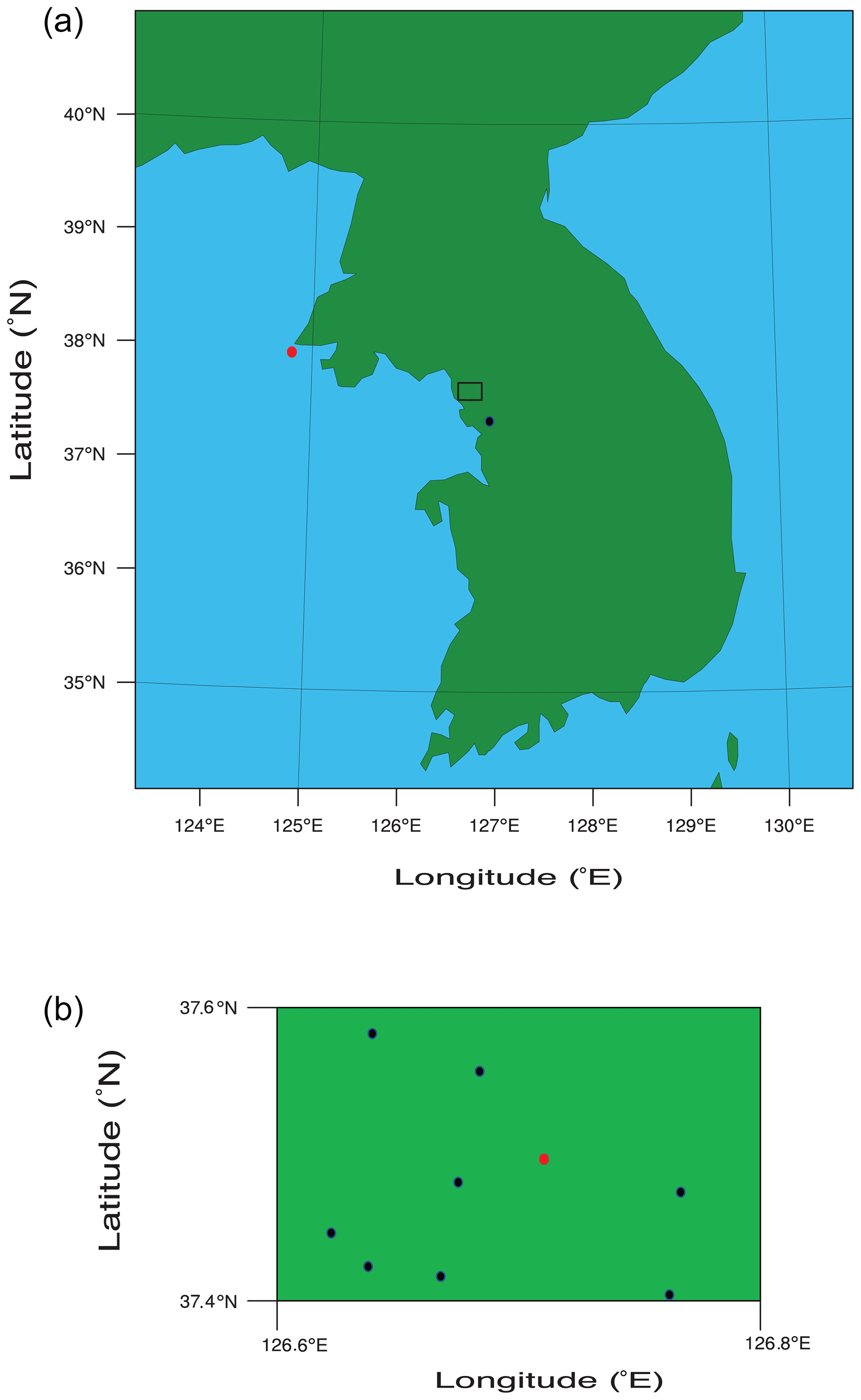
Figure 1(a) An inner rectangle on the map of the Korean Peninsula represents the simulation domain. The green represents the land area and the light blue the ocean area on the map. A black dot marks the location of a site where the radiosonde sounding is obtained and a red dot the location of the PM2.5 station in the Yellow Sea. (b) The simulation domain is shown. The black dots mark the locations of the PM2.5 stations and the red dot the location of the AERONET site in the domain.
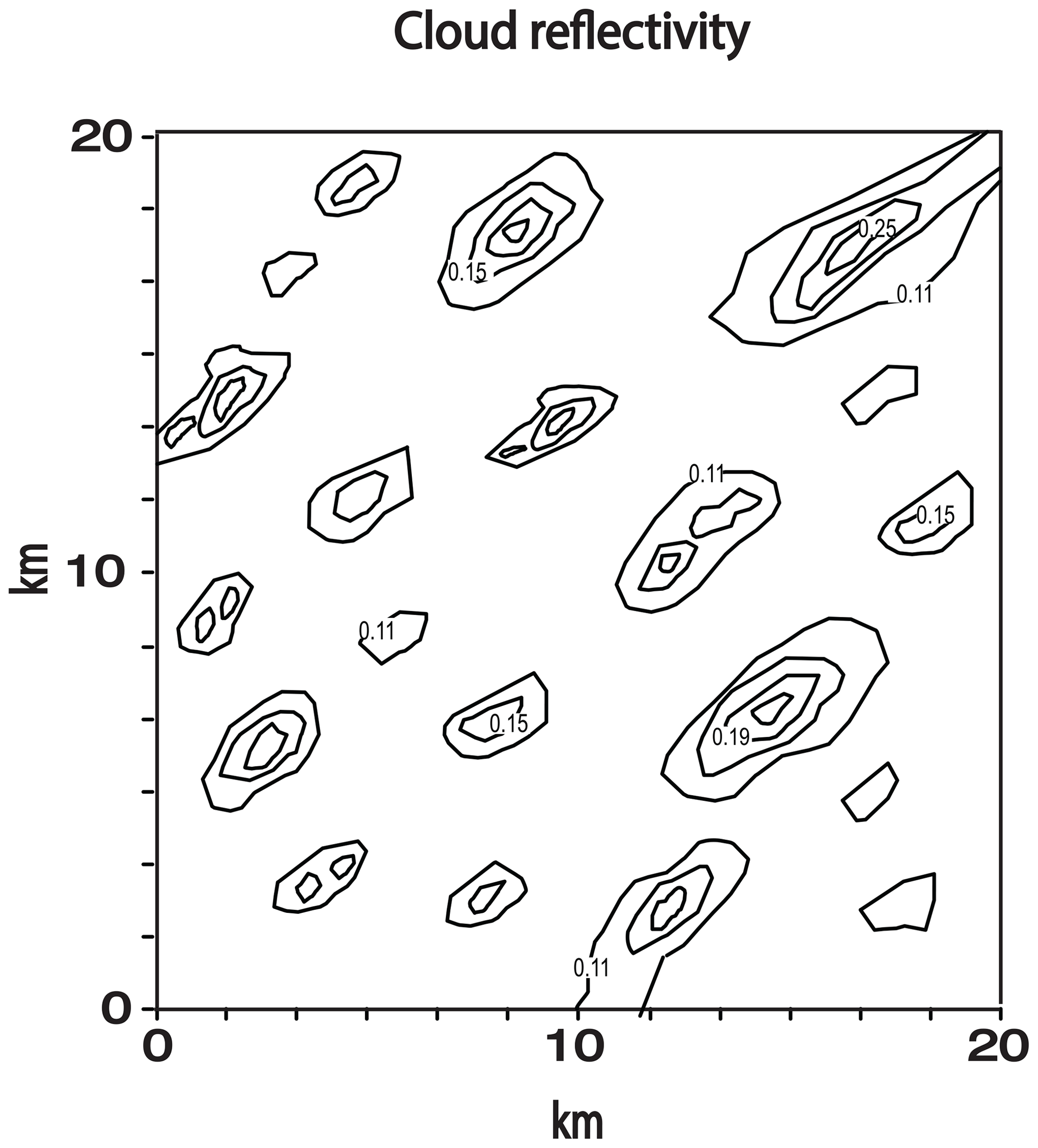
Figure 2Spatial distribution of cloud reflectivity, which is unitless and observed by the COMS at 14:00 LST on 13 April 2016 in the simulation domain. Contours are at 0.11, 0.15, 0.19 and 0.25.
The simulation is performed for a period between 10:00 and 18:00 LST on 13 April 2016. This period includes a time span over which the system exists. For the simulation (i.e., the control run), the length of the domain in both the east–west and north–south directions is 20 km and the model top is at ∼4.5 km in altitude. The time step or temporal resolution is set at 0.1 s. Initial and boundary conditions of potential temperature, specific humidity and wind for the simulation are provided by reanalysis data. These data represent the synoptic-scale environment and are produced by the Met Office Unified Model (Brown et al., 2012) every 6 h on a grid. Figure 3 depicts the vertical distributions of potential temperature and water vapor mixing ratio at 09:00 LST on 13 April 2016 in a radiosonde sounding obtained near the domain as marked in Fig. 1a. This vertical distribution represents initial environmental conditions for the control run. The conditional instability is present in the vertical profiles, and this favors the development of warm cumulus clouds. An open lateral boundary condition is employed for the run.
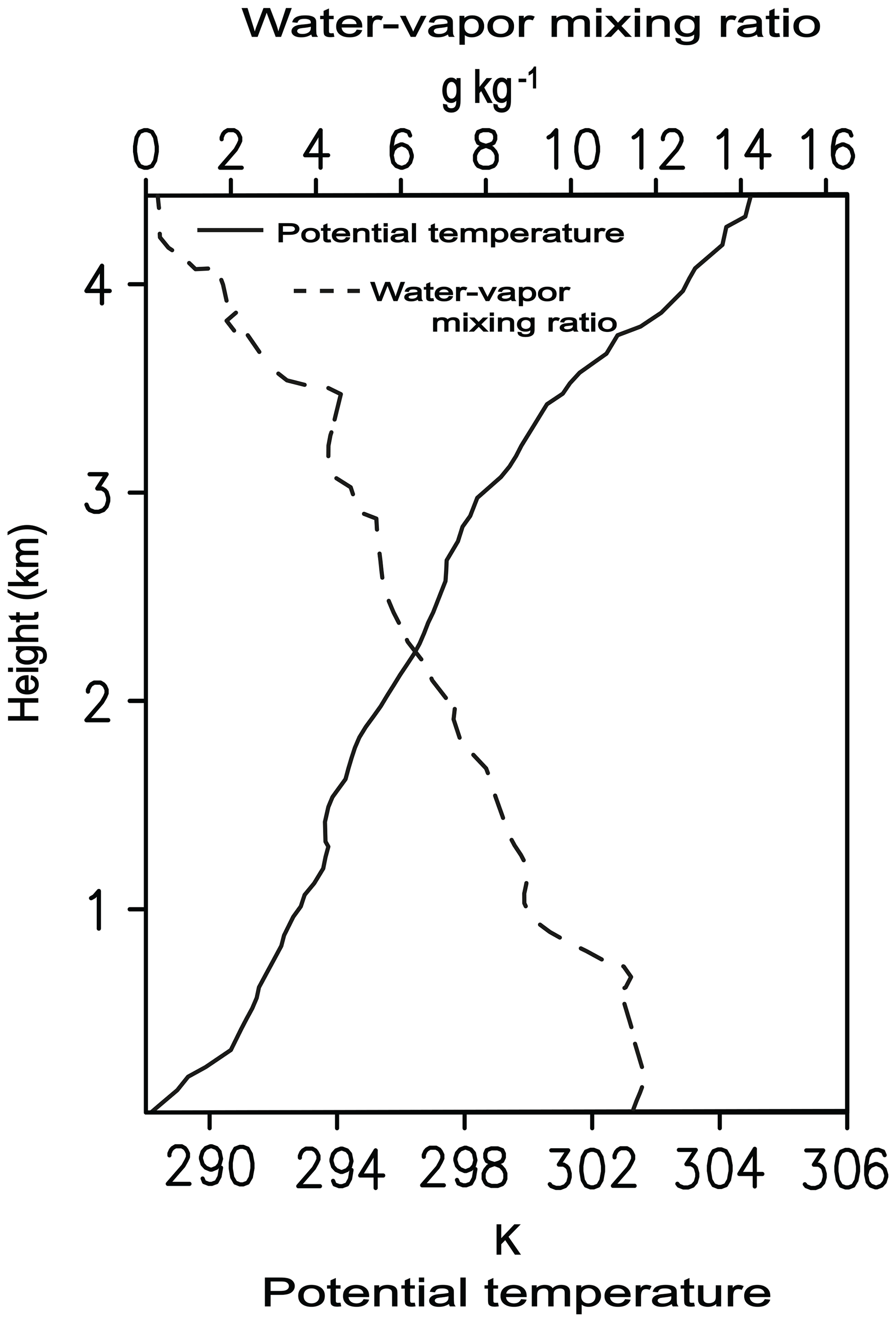
Figure 3Vertical distributions of potential temperature and water vapor mixing ratio at 09:00 LST on 13 April 2016. These distributions are obtained from a radiosonde sounding near the simulation domain in Fig. 1a.
A site of the aerosol robotic network (AERONET; Holben et al., 2001), in addition to ground stations that measure PM2.5, is in the domain as marked in Fig. 1b. The mass of aerosols with diameter smaller than 2.5 µm per unit volume of the air is PM2.5. Around 07:00 LST on 13 April 2016, an aerosol layer advected from East Asia starts to be present in the domain. This advection of aerosols is monitored and identified by PM2.5, which is measured by stations in the Yellow Sea and domain (Eun et al., 2016; Ha et al., 2019; Lee et al., 2021). The station in the Yellow Sea is marked in Fig. 1a. Figure 4 shows the evolution of PM2.5 at the station in the Yellow Sea and the average PM2.5 over stations in the domain from 03:00 to 18:00 LST on 13 April 2016. Due to the aerosol layer advection from East Asia, aerosol mass starts to increase around 04:00 LST and reaches its peak around 08:00 LST at the station in the sea. Then, in the domain, aerosol mass starts to increase around 07:00 LST, and the mass attains its peak around 11:00 LST. This depicts a situation in which aerosol or an aerosol layer advected from East Asia first arrives at the station in the Yellow Sea around 04:00 LST and is then further advected to the east to reach the domain and to start the increase in aerosol mass there around 07:00 LST.
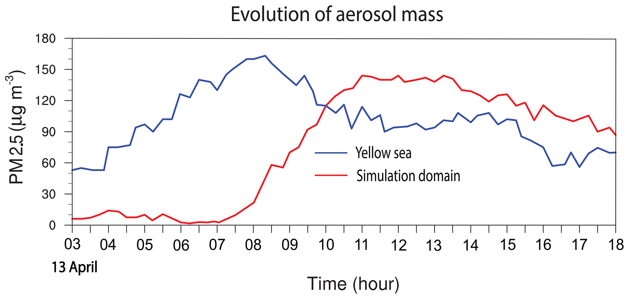
Figure 4Time series of PM2.5 observed at the station in the Yellow Sea (blue line) and of the average PM2.5 over stations in the simulation domain (red line) between 03:00 and 18:00 LST on 13 April 2016.
According to the AERONET measurement at 12:00 LST, which is ∼1 h before the observed cumulus clouds start to form, aerosol particles in the advected aerosol layer, on average, are an internal mixture of 70 % ammonium sulfate, 22 % organic compound and 8 % black carbon. Aerosol chemical composition in this study is assumed to be represented by this mixture in the whole domain during the whole simulation period. Based on the AERONET observation, the shape of the initial size distribution of aerosols acting as CCN is assumed to follow a bimodal lognormal distribution as shown in Fig. 5 in all parts of the domain. The modal radius of this distribution is 0.11 and 1.20 µm, and the standard deviation of this distribution is 1.71 and 1.92, while the partition of aerosol number, which is normalized by the total aerosol number of the size distribution, is 0.999 and 0.001 for accumulation and coarse modes, respectively. The total aerosol number concentration in the advected aerosol layer based on the AERONET-observed size distribution is ∼15 000 cm−3. This concentration is applied to all grid points in the aerosol layer at the first time step of the control run. This aerosol layer is idealized to be located around or below cloud bases between the surface and 1.0 km in the planetary boundary layer (PBL). Cloud bases are located around 1.0 km. At 06:00 LST, ∼1 h before the advected aerosol layer starts to be present, the AERONET-measured aerosol concentration is ∼150 cm−3 in the domain. This aerosol concentration is assumed to be a background aerosol concentration that is not affected by the advected aerosol layer. Based on this assumption, the initial aerosol concentration is set at 150 cm−3 outside the layer.
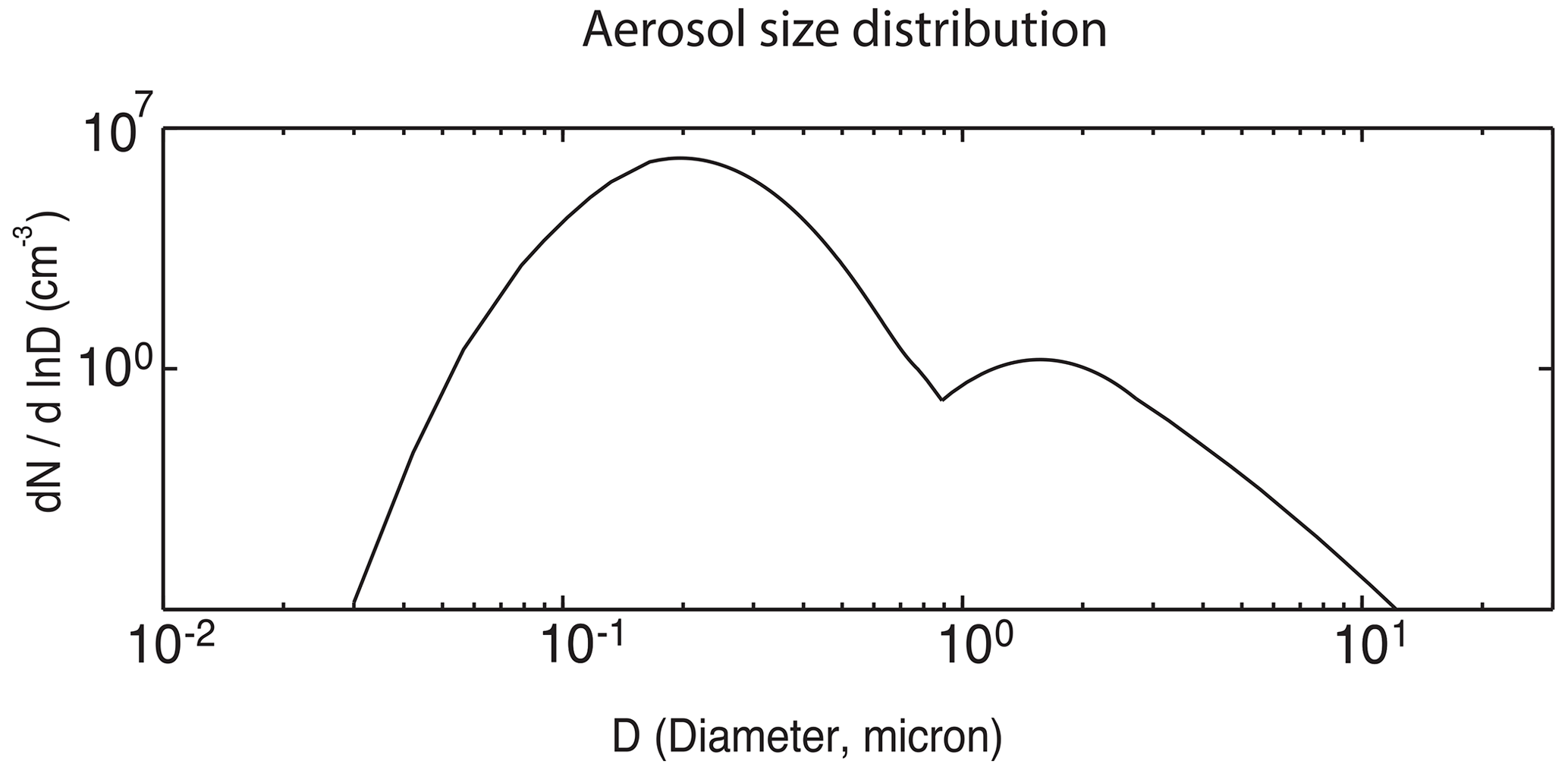
Figure 5Aerosol size distribution at the surface. N represents aerosol number concentration per unit volume of air and D represents aerosol diameter.
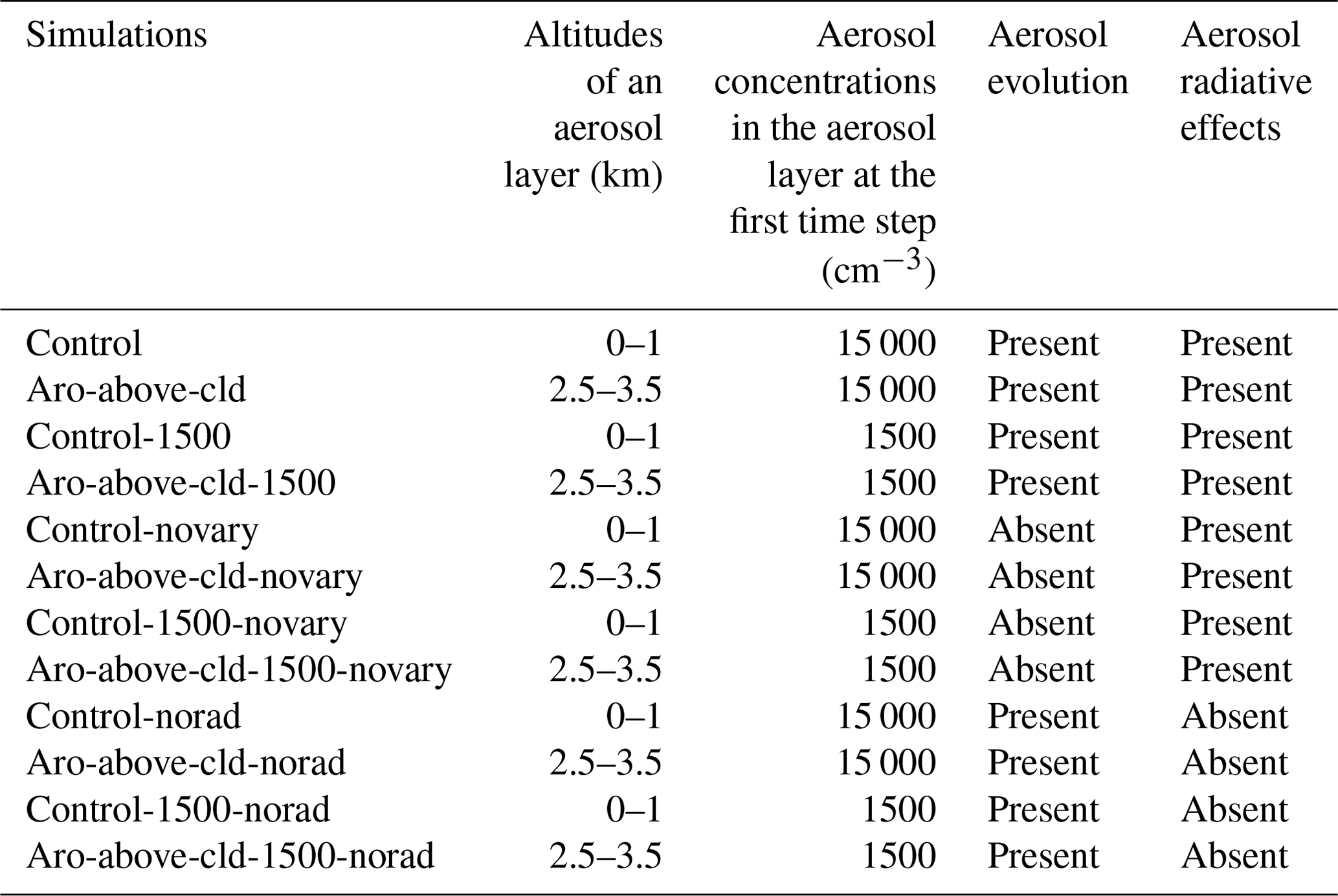
This study compares aerosol effects on warm cumulus clouds when the aerosol layer is above or around the cloud tops to effects when the layer is around or below the cloud bases. For this, we repeat the control run by moving the aerosol layer upward to altitudes between 2.5 and 3.5 km in the free atmosphere, which is above the PBL. Here, initial aerosol concentrations in and outside the aerosol layer are 15 000 and 150 cm−3, respectively, in both of the runs. Altitudes between 2.5 and 3.5 km are places where cloud tops are located frequently, and the simulated maximum cloud-top height is 3.3 km. This repeated run is referred to as the aro-above-cld run.
It is well-known that aerosol–cloud–radiation interactions are strongly dependent on aerosol concentrations (Tao et al., 2012). Hence, we want to test how results in the control and aro-above-cld runs are sensitive to aerosol concentrations in the aerosol layer. For the test, the control and aro-above-cld runs are repeated with 10 times lower initial aerosol concentrations in the aerosol layer but with no changes in initial aerosol concentrations outside the layer. In these repeated runs, the aerosol concentration in the aerosol layer at the first time step is 1500 cm−3. Henceforth, the repeated control and aro-above-cld runs are referred to as the control-1500 and aro-above-cld-1500 runs.
2.2.2 Additional simulations
Clouds affect aerosols through cloud processes such as nucleation of droplets and aerosol transportation (or advection) by cloud-induced wind. Updrafts and downdrafts comprise cloud-induced wind and transport aerosols upward and downward, respectively. Motivated by this, we take interest in impacts of clouds on aerosols and how these impacts in turn change the influence of aerosols on clouds. To examine this aspect of aerosol–cloud interactions, the abovementioned four standard simulations (i.e., the control, aro-above-cld, control-1500 and aro-above-cld-1500 runs) are repeated. In these repeated runs, aerosol concentrations at each grid point, which are set at the first time step, do not vary with time or are not affected by cloud processes. These repeated runs are referred to as the control-novary, aro-above-cld-novary, control-1500-novary and aro-above-cld-1500-novary runs. By comparing the standard simulations to these repeated ones, we aim to identify how cloud processes affect the aerosol layer and then the impacts of the layer on clouds.
In this study, we also aim to better understand the roles of the interception (e.g., reflection, scattering and absorption) of radiation by aerosols in impacts of the aerosol layer on clouds. This interception of radiation by aerosols, which is referred to as aerosol radiative effects, results in phenomena such as radiative heating of air by aerosols. To better understand roles of aerosol radiative effects, the above four standard simulations are repeated again by turning off aerosol radiative effects. These repeated runs are the control-norad, aro-above-cld-norad, control-1500-norad and aro-above-cld-1500-norad runs. The summary of simulations in this study is given in Table 1.
3.1 The control and aro-above-cld runs
Figure 6 depicts the simulated field of the cloud reflectivity at 14:00 LST on 13 April 2016 in the control run. Similar to the observed counterpart in Fig. 2, simulated cloud cells are elongated in the southwest–northeast direction. Also, there is good consistency in the overall cell size and population as well as the overall pattern of the spatial distribution of cloud cells between the observed and simulated fields. Table 3 shows comparisons of cloud and environmental variables between observations and the control run. Observations are performed by ground stations and satellites. Note that ground stations which measure PM2.5 as marked in Fig. 1b also measure cloud and environmental variables. Table 3 shows that differences in those variables between observations and the control run are ∼10 %. This and Fig. 6 indicate that the control run can be considered to have performed reasonably well.
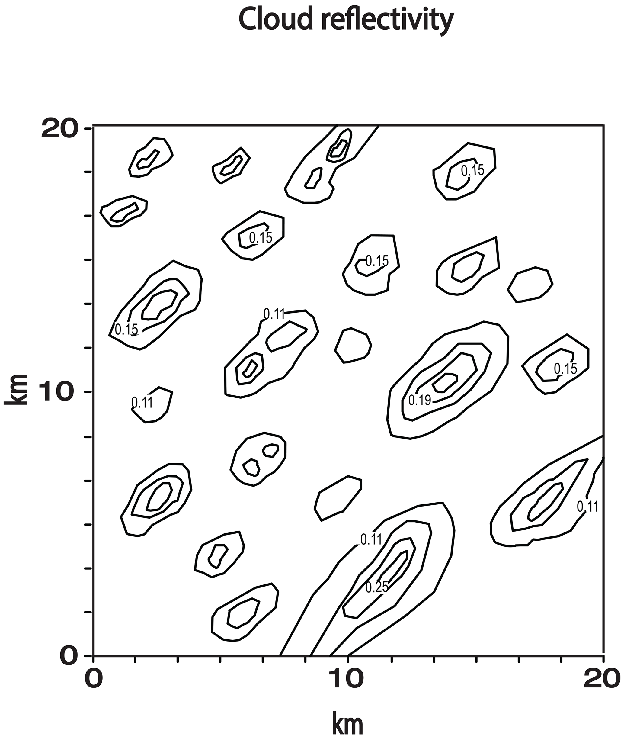
Figure 7 shows the time- and area-averaged vertical distributions of cloud liquid mass density for the standard simulations. In Fig. 7, the cloud layer is between 1.0 and 3.3 km in the control run and between 0.8 and 2.6 km in the aro-above-cld run. The time- and domain-averaged cloud liquid mass density is 0.7 and g m−3 in the control run and in the aro-above-cld run, respectively. Hence, we see that clouds are thicker with higher tops and have greater mass in the control run than in the aro-above-cld run.
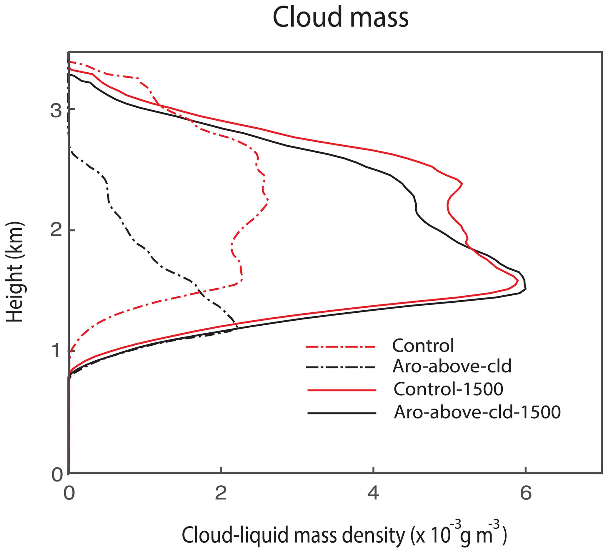
Figure 7Vertical distributions of the time- and area-averaged cloud liquid mass density that represents cloud mass for the standard simulations (i.e., the control, aro-above-cld, control-1500 and aro-above-cld-1500 runs).
Figure 8Time series of the domain-averaged (a) liquid water path, (b) updraft speed, (c) condensation rate and (d) CAPE in the standard simulations.
Table 2The time- and area-averaged net solar radiation, latent heat, sensible heat and total heat (sensible plus latent heat) fluxes at the surface over the whole simulation period in the standard simulations. The numbers in parentheses are averaged over the initial period between 10:00 and 13:50 LST for the control and aro-above-cld runs.

Table 3The simulated and observed values of cloud and environmental variables and the observation sources that have been used to obtain the observed values. At each observation time (simulation time step), cloud fraction (CF) is averaged (obtained) over ground stations (grid points) in the domain as shown in Fig. 1b, and the averaged (obtained) CF is averaged over the simulation period with clouds to calculate the presented and observed (simulated) CF values. To obtain the presented values of cloud-top height (CTH), cloud-bottom height (CBH), cloud optical depth (COD), droplet effective radius (re) and liquid water path (LWP), the observed values at observation spatial points (the simulated values in grid columns for CTH, CBH and LWP and at grid points for COD and re) in the domain are averaged over areas with nonzero values at each observation time (simulation time step) and then over the simulation period with nonzero values. To obtain the presented and simulated values of the surface wind speed (WS), the surface wind direction (WD) and the surface air temperature (ST), the simulated values are averaged over grid points, which correspond to the atmosphere immediately above the surface, and the whole simulation period. To obtain the presented and observed values of those surface variables, the observed values are averaged over ground stations and the whole simulation period.
Figure 8a shows the time series of the domain-averaged liquid water path, which is the vertical integral of cloud liquid mass density, for the standard simulations. During the initial stage of the cloud development between 12:50 and 13:50 LST, the average cloud mass is slightly higher in the control run than in the aro-above-cld run. Also, the average nonzero cloud mass starts to appear earlier in the control run. Over the period between 13:50 and 14:10 LST, there is a jump (or rapid increase or surge) in the average cloud mass in the control run but not in the aro-above-cld run. During this period with the jump, at some specific time points, the average mass is ∼1 order of magnitude higher in the control run. It is of interest that just after the jump and at 14:10 LST, the average mass in the control run starts to decrease and at 14:40 LST becomes lower than that in the aro-above-cld run. Hence, the greater time- and domain-averaged cloud mass in the control run is mainly attributed to the jump. Figure 8b and c show the time series of the domain-averaged updraft speed and condensation rates, respectively. These panels indicate that the average updraft mass fluxes and associated condensation rates in the control run are also slightly higher than in the aro-above-cld run for the period between 12:50 and 13:50 LST. The average updraft speed and associated condensation rates jump and are thus much higher in the control run during the period between ∼ 13:50 and ∼ 14:10 LST (Fig. 8b and c). After the jump, the speed and rates decrease rapidly and become lower in the control run (Fig. 8b and c). Condensation is the only source of cloud mass in warm cumulus clouds. Also, updrafts with higher speeds tend to produce higher condensation rates for a given environmental condition. Hence, cloud mass, condensation rate and the updraft speed are closely linked to each other. This enables cloud mass, condensation rate and the updraft speed to be similar in terms of their temporal evolution in each of the control and aro-above-cld runs (Fig. 8a–c).
Figure 8d shows the time series of the domain-averaged convective available potential energy (CAPE) for the control and aro-above-cld runs. Considering that updrafts grow by consuming buoyancy energy, updraft intensity is proportional to CAPE, which is the integral of the buoyancy energy in the vertical domain. Hence, the evolution of CAPE is similar to that of the updraft speed, associated condensation rates and cloud mass (Fig. 8). This involves the jump not only in CAPE but also in speed, rates and mass in the control run.
In Fig. 8, the peaks (or the maximum values) of the domain-averaged CAPE, the updraft speed, condensation rates and cloud mass in the control run occur around 14:10 LST, and this occurrence is earlier than that which occurs around 14:50 LST in the aro-above-cld run. This means that the cloud system in the control run reaches its mature stage earlier. Immediately after the peak around 14:10 LST, the system enters its dissipating stage in the control run. However, the system enters its dissipating stage after 14:50 LST in the aro-above-cld run. Hence, the cloud system in the control run matures and dissolves faster. Stated differently, the cloud system in the control run has a shorter life cycle.
To find mechanisms controlling the jump in CAPE, which is a main cause of the greater cloud mass in the control run, an analysis of the results is done for an initial period between 10:00 and 13:50 LST, which is immediately before the jump starts to occur. The average net shortwave fluxes at the surface are shown in Table 2 for the initial period in the control and aro-above-cld runs. Table 2 shows that during the initial period, there is a smaller amount of surface-reaching shortwave radiation in the control run than in the aro-above-cld run. The aerosol layer intercepts solar radiation and reduces the surface-reaching solar radiation. In spite of the fact that the initial depth of the aerosol layer and aerosol concentrations in the layer are identical between the runs, results here indicate that the aerosol layer in the atmosphere around or below cloud bases is more efficient in the interception of solar radiation than that in the atmosphere around or above cloud tops. Due to less solar radiation reaching the surface, the time- and area-averaged net surface heat fluxes, which are the sum of the surface sensible and latent-heat fluxes, become lower in the control run during the initial period (Table 2). Hence, the surface fluxes favor more instability or higher CAPE and associated subsequent more intense updrafts and more cloud mass in the aro-above-cld run.
The vertical distributions of the time- and domain-averaged radiative heating rates are obtained for the initial period. For the initial period, the average radiative heating rate is much higher in the control run than in the aro-above-cld run, particularly at altitudes between 0.0 and ∼1.0 km where cloud bases are located (Fig. 9a). This is associated with the fact that the aerosol layer is located at altitudes between 0.0 and 1.0 km in the control run. This more radiative heating in the PBL during the initial period results in the subsequent jump in CAPE, associated higher CAPE, more intense updrafts and more cloud mass after the initial period by outweighing the lower surface heat fluxes in the control run. The aerosol layer is located at altitudes between 2.5 and 3.5 km; hence, the average radiative heating rate is higher around those altitudes in the aro-above-cld run (Fig. 9a and b). However, this higher radiative heating rate is in the upper part of the domain and tends to induce more stabilization of the atmosphere in the aro-above-cld run. Thus, the higher radiative heating rate in the aro-above-cld run contributes to lower CAPE, less intense updrafts and less cloud mass in the aro-above-cld run, especially for the period when the jumps occur in the control run.
Figure 9Vertical distributions of the time- and area-averaged radiative heating rate (a) in the control and aro-above-cld runs over the initial period between 10:00 and 13:50 LST, (b) in the control and aro-above-cld runs, and (c) in the control-1500 and aro-above-cld-1500 runs over the whole simulation period.
3.2 Comparisons between simulations with different aerosol concentrations
With the lower concentration of aerosols in the aerosol layer, there is the much more surface-reaching solar radiation and resultant higher surface fluxes in the control-1500 run than in the control run and in the aro-above-cld-1500 run than in the aro-above-cld run (Table 2). This induces higher CAPE, stronger updrafts, and more condensation and cloud mass in the control-1500 run than in the control run over most of the simulation period except for the period with the jump in CAPE in the control run and in the aro-above-cld-1500 run than in the aro-above-cld run throughout the simulation period (Fig. 8). This leads to the greater time- and domain-averaged cloud mass in the control-1500 run than in the control run and in the aro-above-cld-1500 run than in the aro-above-cld run (Fig. 7). Regarding the control and control-1500 runs, this is despite the fact that aerosol radiative heating in the PBL is higher due to higher aerosol concentrations there in the control run than in the control-1500 run (Fig. 9). Regarding the aro-above-cld-1500 and the aro-above-cld runs, the greater time- and domain-averaged cloud mass is contributed by lower aerosol concentrations and less aerosol radiative heating in the free atmosphere in the aro-above-cld-1500 run than in the aro-above-cld run (Fig. 9). Figure 7 shows that the time- and domain-averaged cloud mass in the aro-above-cld-1500 run is higher than in the control run. This is due to more solar radiation reaching the surface in the aro-above-cld-1500 run (Table 2). The higher average cloud mass in the aro-above-cld-1500 run is despite higher aerosol concentrations and more aerosol radiative heating not only in the PBL in the control run, but also in the free atmosphere in the aro-above-cld-1500 run (Fig. 9). Figure 7 also shows that the time- and domain-averaged cloud mass in the control-1500 run is higher than in the aro-above-cld run. This is associated with the fact that more solar radiation reaches the surface in the control-1500 run than in the aro-above-cld run (Table 2). The higher average cloud mass in the control-1500 run is also associated with higher aerosol concentrations and more aerosol radiative heating not only in the PBL in the control-1500 run, but also in the free atmosphere in the aro-above-cld run (Fig. 9).
Similar to the situation between the control and aro-above-cld runs, there is the less surface-reaching solar radiation in the control-1500 run than in the aro-above-cld-1500 run (Table 2). In association with this, there is less surface heat flux in the control-1500 run. However, overall, CAPE is higher and cloud mass is greater in the control-1500 run than in the aro-above-cld-1500 run (Figs. 7, 8a and d). This is because, similar to the situation between the control and aro-above-cld runs, aerosols heat up the PBL more in the control-1500 run and the free atmosphere more in the aro-above-cld-1500 run (Fig. 9c). The CAPE evolution shows that there is no jump in CAPE and thus updrafts in the control-1500 run (Fig. 8b and d). This mainly contributes to smaller differences in CAPE, updrafts, condensation and cloud mass between the control-1500 and aro-above-cld-1500 runs than between the control and aro-above-cld runs (Figs. 7 and 8).
In the control run, the instability or CAPE accumulates or increases rapidly to reach its peak for a period between 13:50 and 14:10 LST, while in the control-1500 run, CAPE increases gradually to reach its peak from ∼ 12:00 to ∼ 14:30 LST (Fig. 8d). For a period between ∼ 14:10 and ∼ 14:50 LST, CAPE is rapidly reduced back down to the CAPE value around ∼ 13:50 LST in the control run. However, CAPE decreases gradually and never drops back to the CAPE value at ∼ 12:00 LST until the end of the simulation period in the control-1500 run. This leads to the shorter life cycle or lifetime of the system in the control run than in the control-1500 run as well as in the aro-above-cld run. Accompanying this is the similar life cycle between the control-1500 and aro-above-cld-1500 runs. Here, we see that as aerosol concentration increases in the aerosol layer in the atmosphere around or below cloud bases, the timescale of the accumulation and consumption of the instability or convective energy gets shorter, leading to the shorter lifetime of the cloud system.
3.3 Comparisons between simulations with predicted and prescribed aerosol concentrations
Figure 10 shows the vertical distributions of aerosol concentrations, which are averaged over the horizontal domain and simulation period, for the standard and repeated runs with no temporal variation of aerosols. Comparisons between the control and control-novary runs and between the control-1500 and control-1500-novary runs show that due to the upward transportation of aerosols by updrafts, aerosol concentrations in the aerosol layer in the PBL are reduced and those in the air above the layer increase (Fig. 10a and c). Note that the PBL is where cloud-induced updrafts develop and grow; hence, the upward transportation of aerosols by them is dominant. This leads to more PBL radiative heating of air by aerosols in the control-novary run than in the control run and in the control-1500-novary run than in the control-1500 run.
Figure 10Vertical distributions of the time- and area-averaged aerosol concentrations (a) in the control and control-novary runs, (b) aro-above-cld and aro-above-cld-novary runs, (c) control-1500 and control-novary-1500 runs, and (d) aro-above-cld-1500 and aro-above-cld-novary-1500 runs.
Comparisons between the aro-above-cld and aro-above-cld-novary runs and between the aro-above-cld-1500 and aro-above-cld-1500-novary runs show that due to the transportation of aerosols by downdrafts, aerosol concentrations in the aerosol layer in the free atmosphere are reduced and those in the air below the layer increase (Fig. 10b and d). Note that the free atmosphere, which includes the above-PBL atmosphere around or above cloud tops, is where cloud-induced updrafts decelerate and turn into downdrafts, and the downward transportation of aerosols by them is dominant. However, those increases in aerosol concentrations in the air below the aerosol layer mainly occur between ∼1.5 and ∼2.5 km, and aerosol concentrations and the associated instability in the PBL do not change significantly (Fig. 10b and d). This leads to similar instability in the PBL and CAPE, which in turn leads to similar updrafts and cloud mass between the aro-above-cld and aro-above-cld-novary runs and between the aro-above-cld-1500 and aro-above-cld-1500-novary runs (Fig. 11a).
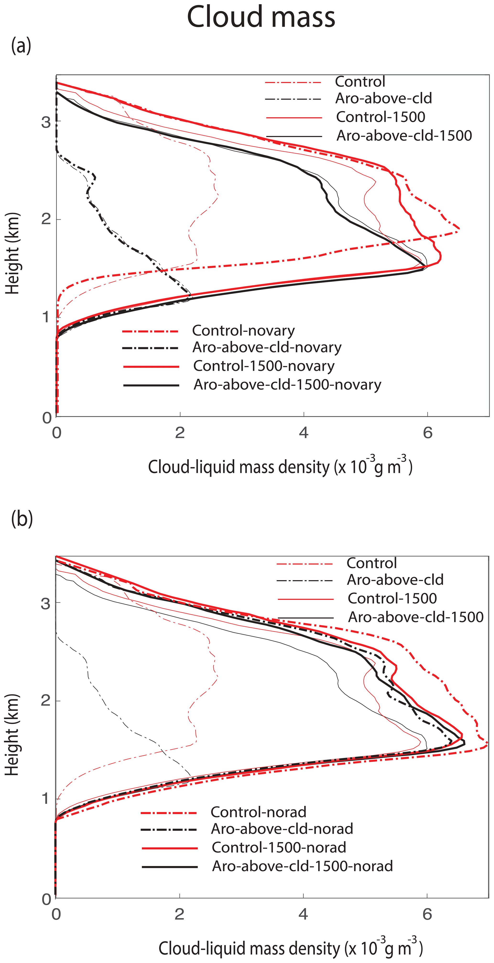
Figure 11Vertical distributions of the time- and area-averaged cloud liquid mass density. The control-novary, aro-above-cld-novary, control-1500-novary and aro-above-cld-1500-novary runs (a) as well as the control-norad, aro-above-cld-norad, control-1500-norad and aro-above-cld-1500-norad runs (b) are shown together with the standard simulations.
Due to more radiative heating of air in the PBL, there is higher CAPE, stronger updrafts and higher cloud mass in the control-novary run than in the control run and in the control-1500-novary run than in the control-1500 run (Fig. 11a). It is notable that cloud mass in the control-novary run is so large that its maximum value in the vertical profile exceeds that even in the control-1500-novary run (Fig. 11a). Associated with this, there are only ∼20 % changes in cloud mass between the control-1500 and control-1500-novary runs, while there are as much as ∼200 % changes in cloud mass between the control and control-novary runs. This indicates that with higher aerosol concentrations in the PBL, changes in cloud mass due to the wind-induced variation of those concentrations are much larger.
3.4 Comparisons between simulations with and without aerosol radiative effects
Figure 11b shows that with no aerosol radiative effects, differences in cloud mass due to the altitude of the aerosol layer are smaller. However, even with no aerosol radiative effects, there is higher cloud mass when the aerosol layer is in the PBL than in the free atmosphere as in the standard runs. Also, cloud mass increases when aerosol radiative effects are turned off, and this increase is enhanced as aerosol concentrations increase (Fig. 11b). Here, we see that aerosol radiative effects suppress clouds and reduce cloud mass by reducing the surface-reaching solar radiation and the surface heat fluxes. The suppression of clouds and reduction in cloud mass are greater with higher aerosol concentrations, since more aerosols reduce the surface-reaching solar radiation more.
Note that aerosol activation mainly occurs around cloud bases in the PBL, and more aerosols induce more activation for a given thermodynamic condition. Hence, there is more aerosol activation (or nucleation of droplets) and higher cloud droplet number concentration (CDNC) when the aerosol layer is in the PBL than in the free atmosphere. The averaged CDNC over grid points with nonzero CDNC and the whole simulation period is 532, 57, 131 and 53 cm−3 in the control-norad, aro-above-cld-norad, control-1500-norad and aro-above-cld-1500-norad runs, respectively. Droplets act as a source of condensation, since individual droplets provide surface areas onto which water vapor condenses. Hence, higher CDNC induces more condensation, and this in turn induces stronger updrafts and more cloud mass with the aerosol layer in the PBL than in the free atmosphere. These effects of more aerosols, which induce more condensation and stronger updrafts, are generally referred to as aerosol microphysical effects (Lee et al., 2016). The differences in CDNC due to the altitude of the aerosol layer increase with increasing aerosol concentrations. This leads to greater differences in condensation, associated updrafts and cloud mass due to the altitude of the aerosol layer with higher aerosol concentrations when there are no aerosol radiative effects (Fig. 11b).
Here, we see that differences in cloud mass due to the altitude of the aerosol layer are greater when aerosol microphysical and radiative effects work together than when aerosol microphysical effects work alone (Fig. 11b). Also, remember that the initial concentration of aerosols in the aro-above-cld-norad run is identical to that in the aro-above-cld-1500-norad run in the PBL. Due to this, CDNC, condensation and cloud mass in the aro-above-cld-norad run are similar to those in the aro-above-cld-1500-norad run (Fig. 11b).
This study examined how impacts of aerosols on warm cumulus clouds in the Korean Peninsula vary with the altitude of an aerosol layer. It is found that the aerosol layer intercepts the surface-reaching solar radiation more when the layer is in the PBL, which corresponds to the atmosphere around or below cloud bases, than in the free atmosphere, which includes the above-PBL atmosphere around or above cloud tops. With the aerosol layer in the PBL, this makes the surface heat fluxes and associated CAPE lower, which tends to make updrafts weaker and cloud mass lower. However, the layer in the PBL heats up the air there more to produce the higher CAPE and cloud mass.
With decreasing concentrations of aerosols in the aerosol layer, there are decreases in the interception of the surface-reaching solar radiation and increases in surface heat fluxes, CAPE and cloud mass. However, the decreasing concentrations of aerosols cause the jump in CAPE to disappear when the layer is in the PBL. This reduces differences in cloud mass due to the altitude of the layer. When the aerosol layer is in the PBL, with increasing aerosol concentrations in the layer, the lifetime of cloud system is reduced and becomes shorter than when the layer is in the free atmosphere.
Updrafts and downdrafts in clouds transport aerosols. In particular, for the aerosol layer in the PBL, updrafts transport aerosols in the layer to places above it. This reduces aerosol concentrations in the layer, leading to reduction in radiative heating of air by aerosols, CAPE, updrafts and cloud mass. This reduction is enhanced with increasing aerosol concentrations in the layer. For the aerosol layer in the free atmosphere, downdrafts transport aerosols in the layer to places below it. However, this does not affect aerosol concentrations and radiative heating of air in the PBL significantly. This in turn has negligible effects on CAPE and cloud mass.
Aerosol radiative effects suppress clouds and reduce cloud mass by cutting down the surface-reaching solar radiation. This suppression of clouds increases with increasing aerosol concentrations in the aerosol layer. Aerosol microphysical effects enhance cloud mass, and these effects are stronger with higher aerosol concentrations. Differences in cloud mass due to the altitude of the aerosol layer are enhanced when aerosol radiative effects and aerosol microphysical effects work together compared to when only aerosol microphysical effects are present.
This study shows that aerosol-induced changes in the surface fluxes and those in radiative heating of air interact with each other in terms of responses of convection and clouds to aerosols. This interaction varies with the altitude of aerosols and cloud-induced wind. In general, traditional parameterizations for warm cumulus clouds in climate and weather forecast models have not been able to consider this dependence of the interaction on the altitude of aerosols, since those parameterizations do not differentiate aerosol layers based on their vertical locations. In addition, the cloud-induced wind at cloud scales has not been represented by those parameterizations with good confidence. So, impacts of aerosol transportation by cloud-induced wind on the interaction have not been properly considered in traditional parameterizations. This suggests that the vertical locations of aerosols and cloud-induced wind should be added to factors that need to be considered or improved to better parameterize warm cumulus clouds and their interactions with aerosols.
Our private computer system stores the code and data, which are private and used in this study. Upon approval from funding sources, the data will be open to the public. Projects related to this paper have not been finished, and thus the sources currently prevent the data from being open to the public. However, if information on the data is needed, contact the corresponding author Seoung Soo Lee (slee1247@umd.edu).
Essential initiative ideas were provided by SSL, JU and WJC to start this work. Simulation and observation data were analyzed by SSL, JU and KJH. CHJ, JG and YZ reviewed the results and contributed to their improvement.
The contact author has declared that none of the authors has any competing interests.
Publisher's note: Copernicus Publications remains neutral with regard to jurisdictional claims in published maps and institutional affiliations.
The authors thank the anonymous reviewers for valuable comments on this paper.
This study is supported by a National Research Foundation of Korea (NRF) grant funded by the Korean government (MSIT) (grant nos. NRF2020R1A2C1003215 and 2020R1A2C1013278) and the Korea Institute of Marine Science and Technology Promotion (KIMST) funded by the Ministry of Oceans and Fisheries (20210607). This study is also supported by the Basic Science Research Program through the NRF funded by the Ministry of Education (grant no. 2020R1A6A1A03044834), the FRIEND (Fine Particle Research Initiative in East Asia Considering National Differences) project through the NRF funded by the Ministry of Science and ICT (grant no. 2020M3G1A1114617), and a National Research Foundation of Korea (NRF) grant funded by the Korean government (grant no. NRF-2021R1F1A1046878).
This paper was edited by Jianping Huang and reviewed by four anonymous referees.
Albrecht, B. A.: Aerosols, cloud microphysics, and fractional cloudiness, Science, 245, 1227–1230, 1989.
Brown, A., Milton, S., Cullen, M., Golding, B., Mitchell, J., and Shelly, A.: Unified modeling and prediction of weather and climate: A 25-year journey, B. Am Meteorol. Soc., 93, 1865–1877, 2012.
Chaboureau, J.-P., Labbouz, L., Flamant, C., and Hodzic, A.: Acceleration of the southern African easterly jet driven by the radiative effect of biomass burning aerosols and its impact on transport during AEROCLO-sA, Atmos. Chem. Phys., 22, 8639–8658, https://doi.org/10.5194/acp-22-8639-2022, 2022.
Che, H., Stier, P., Watson-Parris, D., Gordon, H., and Deaconu, L.: Source attribution of cloud condensation nuclei and their impact on stratocumulus clouds and radiation in the south-eastern Atlantic, Atmos. Chem. Phys., 22, 10789–10807, https://doi.org/10.5194/acp-22-10789-2022, 2022.
Chen, F. and Dudhia, J.: Coupling an advanced land-surface hydrology model with the Penn State-NCAR MM5 modeling system. Part I: Model description and implementation, Mon. Weather Rev., 129, 569–585, 2001.
Deaconu, L. T., Ferlay, N., Waquet, F., Peers, F., Thieuleux, F., and Goloub, P.: Satellite inference of water vapour and above cloud aerosol combined effect on radiative budget and cloud top processes in the southeastern Atlantic Ocean, Atmos. Chem. Phys., 19, 11613–11634, https://doi.org/10.5194/acp-19-11613-2019, 2019.
de Graaf, M., Bellouin, N., Tilstra, L. G., Haywood, J., and Stammes, P.: Aerosol direct radiative effect of smoke over clouds over the southeast Atlantic Ocean from 2006 to 2009, Geophys. Res. Lett., 41, 7723–7730, 2014.
Denjean, C., Bourrianne, T., Burnet, F., Mallet, M., Maury, N., Colomb, A., Dominutti, P., Brito, J., Dupuy, R., Sellegri, K., Schwarzenboeck, A., Flamant, C., and Knippertz, P.: Overview of aerosol optical properties over southern West Africa from DACCIWA aircraft measurements, Atmos. Chem. Phys., 20, 4735–4756, https://doi.org/10.5194/acp-20-4735-2020, 2020.
Eun, S.-H., Kim, B.-G., Lee, K.-M., and Park, J.-S.: Characteristics of recent severe haze events in Korea and possible inadvertent weather modification, Scient. Onl. Lett. Atmos., 12, 32–36, 2016.
Feingold, G., Jiang, H., and Harrington, J. Y.: On smoke suppression of clouds in Amazonia, Geophys. Res. Lett., 32, L02804, https://doi.org/10.1029/2004GL021369, 2005.
Formenti, P., D'Anna, B,. Flamant, C., Mallet, M., Piketh, S. J., Schepanski, K., Waquet, F., Auriol, F., Brogniez, G., Burnet, F., Chaboureau, J. P., Chauvigné, A., Chazette, P., Denjean, C., Desboeufs, K., Doussin, J. F., Elguindi, N., Feuerstein, S., Gaetani, M., Giorio, C. Klopper, D., Mallet, M. D., Nabat, P., Monod, A., Solmon, F., Namwoonde, A., Chikwililwa, C., Mushi, R., Welton, E. J., and Holben, B.: The Aerosols, Radiation and Clouds in Southern Africa Field Campaign in Namibia: Overview, illustrative observations, and way forward, B. Am. Meteorol. Soc., 100, 1277–1298, 2019.
Forster, P., Ramaswamy, V,. Artaxo, P., Berntsen, T., Betts, R., Fahey, D. Haywood, J., Lean, J., Lowe, D., Myhre, G., Nganga, J., Prinn, R., Raga, G., Schulz, M., and Van Dorland, R.: Changes in atmospheric constituents and in radiative forcing, in: Climate change 2007: the physical science basis, Contribution of working group I to the Fourth Assessment Report of the Intergovernmental Panel on Climate Change, edited by: Solomon, S., Qin, D., Manning, M., Chen, Z., Marquis, M., Averyt, K. B., Tignor, M., and Miller, H. L., Cambridge Univ. Press, New York, ISBN 978-0-521-70596-7, 2007.
Ha, K.-J., Nam, S., Jeong, J.-Y., Moon, I.-J., Lee, M., Yun, J., Jang, C. J., Kim, Y. S., Byun, D.-S., Heo, K.-Y., and Shim, J.-S.: Observations utilizing Korean ocean research stations and their applications for process studies, B. Am. Meteorol. Soc., 100, 2061–2075, 2019.
Hahn, C. J. and Warren, S. G.: A gridded climatology of clouds over land (1971–96) and ocean (1954–97) from surface observations worldwide. Numeric Data Package NDP-026EORNL/CDIAC-153, CDIAC, Department of Energy, Oak Ridge, TN, https://doi.org/10.3334/CDIAC/cli.ndp026e, 2007.
Hansen, J. E., Sato, M., and Ruedy, R.: Radiative forcing and climate response, J. Geophys. Res., 102, 6831–6864, 1997.
Hartmann, D. L., Ockert-Bell, M. E., and Michelsen, M. L.: The effect of cloud type on earth's energy balance – Global analysis, J. Climate, 5, 1281–1304, 1992.
Haslett, S. L., Taylor, J. W., Evans, M., Morris, E., Vogel, B., Dajuma, A., Brito, J., Batenburg, A. M., Borrmann, S., Schneider, J., Schulz, C., Denjean, C., Bourrianne, T., Knippertz, P., Dupuy, R., Schwarzenböck, A., Sauer, D., Flamant, C., Dorsey, J., Crawford, I., and Coe, H.: Remote biomass burning dominates southern West African air pollution during the monsoon, Atmos. Chem. Phys., 19, 15217–15234, https://doi.org/10.5194/acp-19-15217-2019, 2019.
Haywood, J. M. and Shine, K. P.: Multi-spectral calculations of the radiative forcing of tropospheric sulfate and soot aerosols using a column model, Q. J. Roy. Meteorol. Soc., 123, 1907–1930, 1997.
Holben, B. N., Tanré, D., Smirnov, A., Eck, T. F., Slutsker, I., Abuhassan, N., Newcomb, W. W., Schafer, J. S., Chatenet, B., Lavenu, F., Kaufman, Y. J., Castle, J. V., Setzer, A., Markham, B., Clark, D., Frouin, R., Halthore, R., Karneli, A., O'Neill, N. T., Pietras, C., Pinker, R. T., Voss, K., and Zibordi, G.: An emerging ground-based aerosol climatology: Aerosol optical depth from AERONET, J. Geophys. Res., 106, 12067–12097, 2001.
Johnson, B. T., Shine, K. P., and Forster, P. M.: The semi-direct aerosol effect: Impact of absorbing aerosols on marine stratocumulus, Q. J. Roy. Meteorol. Soc., 130, 1407–1422, 2004.
Khain, A., Pokrovsky, A., Rosenfeld, D., Blahak, U., and Ryzhkoy, A.: The role of CCN in precipitation and hail in a mid-latitude storm as seen in simulations using a spectral (bin) microphysics model in a 2D dynamic frame, Atmos. Res., 99, 129–146, 2011.
Lee, S. S., Guo, J. M., and Li, Z.: Delaying precipitation by air pollution over the Pearl River Delta. Part II: Model simulations, J. Geophys. Res., 121, 11739–11760, 2016.
Lee, S. S., Ha, K.-J., Manoj, M. G., Kamruzzaman, M., Kim, H., Utsumi, N., Zheng, Y., Kim, B.-G., Jung, C. H., Um, J., Guo, J., Choi, K. O., and Kim, G.-U.: Midlatitude mixed-phase stratocumulus clouds and their interactions with aerosols: how ice processes affect microphysical, dynamic, and thermodynamic development in those clouds and interactions?, Atmos. Chem. Phys., 21, 16843–16868, https://doi.org/10.5194/acp-21-16843-2021, 2021.
Liou, K. N.: An introduction to atmospheric radiation, Academic Press, 583 pp., ISBN 978-01-245-1451-5, 2002.
Mari, C. H., Cailley, G., Corre, L., Saunois, M., Attié, J. L., Thouret, V., and Stohl, A.: Tracing biomass burning plumes from the Southern Hemisphere during the AMMA 2006 wet season experiment, Atmos. Chem. Phys., 8, 3951–3961, https://doi.org/10.5194/acp-8-3951-2008, 2008.
McFarquhar, G. M. and Wang, H.: Effects of Aerosols on Trade Wind Cumuli over the Indian Ocean: Model Simulations, Q. J. Roy. Meteorol. Soc., 132, 821–843, 2006.
Menut, L., Flamant, C., Turquety, S., Deroubaix, A., Chazette, P., and Meynadier, R.: Impact of biomass burning on pollutant surface concentrations in megacities of the Gulf of Guinea, Atmos. Chem. Phys., 18, 2687–2707, https://doi.org/10.5194/acp-18-2687-2018, 2018.
Mlawer, E. J., Taubman, S. J., Brown, P. D., Iacono, M. J., and Clough, S. A.: RRTM, a validated correlated-k model for the longwave, J. Geophys. Res., 102, 16663–16682, 1997.
Ramaswamy, V., Boucher, O., Haigh, J., Hauglustaine, D., Haywood, J., Myhre, G., Nakajima, T., Shi, G. Y., and Solomon, S.: Radiative forcing of climate change, in: Climate Change 2001: The Scientific Basis, edited by: Houghton, J. T., Ding, Y., Griggs, D. J., Noguer, M., van der Linden, P. J., Dai, X., Maskell, K., and Johnson, C. A., Cambridge Univ. Press, New York, 349–416, ISBN 978-0-521-80767-8, 2001.
Redemann, J., Wood, R., Zuidema, P., Doherty, S. J., Luna, B., LeBlanc, S. E., Diamond, M. S., Shinozuka, Y., Chang, I. Y., Ueyama, R., Pfister, L., Ryoo, J.-M., Dobracki, A. N., da Silva, A. M., Longo, K. M., Kacenelenbogen, M. S., Flynn, C. J., Pistone, K., Knox, N. M., Piketh, S. J., Haywood, J. M., Formenti, P., Mallet, M., Stier, P., Ackerman, A. S., Bauer, S. E., Fridlind, A. M., Carmichael, G. R., Saide, P. E., Ferrada, G. A., Howell, S. G., Freitag, S., Cairns, B., Holben, B. N., Knobelspiesse, K. D., Tanelli, S., L'Ecuyer, T. S., Dzambo, A. M., Sy, O. O., McFarquhar, G. M., Poellot, M. R., Gupta, S., O'Brien, J. R., Nenes, A., Kacarab, M., Wong, J. P. S., Small-Griswold, J. D., Thornhill, K. L., Noone, D., Podolske, J. R., Schmidt, K. S., Pilewskie, P., Chen, H., Cochrane, S. P., Sedlacek, A. J., Lang, T. J., Stith, E., Segal-Rozenhaimer, M., Ferrare, R. A., Burton, S. P., Hostetler, C. A., Diner, D. J., Seidel, F. C., Platnick, S. E., Myers, J. S., Meyer, K. G., Spangenberg, D. A., Maring, H., and Gao, L.: An overview of the ORACLES (ObseRvations of Aerosols above CLouds and their intEractionS) project: aerosol–cloud–radiation interactions in the southeast Atlantic basin, Atmos. Chem. Phys., 21, 1507–1563, https://doi.org/10.5194/acp-21-1507-2021, 2021.
Roberts, G. C. and Nenes, A.: A Continuous-Flow Streamwise Thermal-Gradient CCN Chamber for Atmospheric Measurements, Aerosol Sci. Tech., 39, 206–221 https://doi.org/10.1080/027868290913988, 2005.
Stephens, G. L. and Greenwald, T. J.: Observations of the Earth's radiation budget in relation to atmospheric hydrology. Part II: Cloud effects and cloud feedback, J. Geophys. Res., 96, 15325–15340, 1991.
Tao, W.-K., Chen, J.-P., Li, Z., Wang, C., and Zhang C., Impact of aerosols on convective clouds and precipitation, Rev. Geophys., 50, RG2001, https://doi.org/10.1029/2011RG000369, 2012.
van der Werf, G. R., Randerson, J. T., Giglio, L., Collatz, G. J., Mu, M., Kasibhatla, P. S., Morton, D. C., DeFries, R. S., Jin, Y., and van Leeuwen, T. T.: Global fire emissions and the contribution of deforestation, savanna, forest, agricultural, and peat fires (1997–2009), Atmos. Chem. Phys., 10, 11707–11735, https://doi.org/10.5194/acp-10-11707-2010, 2010.
Wang, H., Skamarock, W. C., and Feingold, G.: Evaluation of scalar advection schemes in the Advanced Research WRF model using large-eddy simulations of aerosol-cloud interactions, Mon. Weather Rev., 137, 2547–2558, 2009.
Warren, S. G., Hahn, C. J., London, J., Chervin, R. M., and Jenne, R. L.: Global distribution of total cloud cover and cloud types over land. NCAR Tech. Note NCAR/TN-273+STR, National Center for Atmospheric Research, Boulder, CO, 29 pp. + 200 maps, https://doi.org/10.5065/D6GH9FXB, 1986.
Wilcox, E. M.: Stratocumulus cloud thickening beneath layers of absorbing smoke aerosol, Atmos. Chem. Phys., 10, 11769–11777, https://doi.org/10.5194/acp-10-11769-2010, 2010.
Wood, R.: Stratocumulus clouds, Mon. Weather Rev., 140, 2373–2423, 2012.
Xu, H., Guo, J., Wang, Y., Zhao, C., Zhang, Z., Min, M., Miao, Y., Liu, H., He, J., Zhou, S., and Zhai, P.: Warming effect of dust aerosols modulated by overlapping clouds below, Atmos. Environ., 166, 393–402, 2017.