the Creative Commons Attribution 4.0 License.
the Creative Commons Attribution 4.0 License.
 | 27 Feb 2023
Establishment of an analytical model for remote sensing of typical stratocumulus cloud profiles under various precipitation and entrainment conditions
Huazhe Shang
Souichiro Hioki
Guillaume Penide
Céline Cornet
Jérôme Riedi
Structural patterns of cloud effective radius (ER) and liquid water content (LWC) profiles are essential variables of cloud lifecycle and precipitation processes, while observing cloud profiles from passive remote-sensing sensors remains highly challenging. Understanding whether there are typical structural patterns of ER and LWC profiles in liquid clouds and how they are linked to cloud entrainment or precipitating status is critical in developing algorithms to derive cloud profiles from passive satellite sensors. This study aims to address these questions and provide a preliminary foundation for the development of liquid cloud profile retrievals for the Multi-viewing, Multi-channel and Multi-polarization Imaging (3MI) sensor aboard the European Organization for the Exploitation of Meteorological Satellites (EUMETSAT) Polar System-Second Generation (EPS-SG) satellite, which is scheduled to be launched in 2025. Firstly, we simulate a large ensemble of stratocumulus cloud profiles using the Colorado State University (CSU) Regional Atmospheric Modeling System (RAMS). The empirical orthogonal function (EOF) analysis is adopted to describe the shape of simulated profiles with a limited number of elemental profile variations. Our results indicate that the first three EOFs of LWC and ER profiles can explain >90 % of LWC and ER profiles. The profiles are divided into four prominent patterns and all of these patterns can be simplified as triangle-shaped polylines. The frequency of these four patterns is found to relate to intensities of the cloud-top entrainment and precipitation. Based on these analyses, we propose a simplified triangle-shaped cloud profile parameterization scheme allowing us to represent these main patterns of LWC and ER. This simple yet physically realistic analytical model of cloud profiles is expected to facilitate the representation of cloud properties in advanced retrieval algorithms such as those developed for the 3MI/EPS-SG.
- Article
(9527 KB) - Full-text XML
- BibTeX
- EndNote


Stratocumulus cloud layers extend practically unbroken for tens to hundreds of kilometers and cover approximately 20 % of the low-latitude oceans and 50 % of the subtropical and midlatitude oceans (Wood, 2015). The widespread stratocumulus imposes a negative radiative forcing as it modifies the reflection of shortwave solar radiation more than outgoing longwave radiation because of its low altitude and limited optical thickness (Arabas et al., 2009). The vertical profiles of cloud effective radius (ER) and liquid water content (LWC) inside the stratocumulus layer inferred from satellites are crucial to understanding cloud microphysical processes and to quantifying their radiative impacts on climate. For example, the cloud droplet profile (CDP) helps to interpret when and where the transformation into raindrops starts by coalescence. In addition, the LWC profiles represent the cloud thermodynamic and dynamic structures of the cloud column (Carey et al., 2008).
Cloud profiles characterized by active radars operated on ground-based sites or spaceborne satellites often served as the truth to validate cloud retrievals from passive sensors (Roebeling et al., 2008). Ground-based radars such as the scanning Atmospheric Radiation Measurement (ARM) cloud radars operating at the X band (9.4 GHz), the Ka band (35 GHz), and the W band (94 GHz) are capable of characterizing vertical profiles of cloud reflectivities (Kollias et al., 2014; Lhermitte, 1988). Combined with liquid water path measured by microwave radiometers and cloud base height identified by ceilometers, the profiles of LWC, ER, and cloud droplet number concentration (CDNC) can be estimated (Frisch et al., 1995; Dong and Mace, 2003; Mace and Sassen, 2000; Rémillard et al., 2013). It is also reported that ground-based radar could distinguish drizzle from cloud particles (Chen et al., 2008) and derive the LWC and ER profiles of each feature (Wu et al., 2020). Airborne equipped particle probes, imagers, and spectrometers are able to capture the profile of size distribution and droplet number concentration for cloud and precipitation droplets (Lawson et al., 2001; Dadashazar et al., 2022). Even though uncertainties such as capturing the extremely small or large droplets, unrealistic assumptions, types of probes, and impact from their installations exist in the measurements, these kinds of datasets provide valuable reference for understanding the cloud profiles in nature and evaluating these simulations or satellite retrievals (Grosvenor et al., 2018a; Alexandrov et al., 2020a; Zhao et al., 2018). The spaceborne cloud profiling radar (CPR), e.g., NASA's CloudSat CPR (Stephens et al., 2002) and ESA-JAXA's EarthCARE CPR (Illingworth et al., 2015), are able to detect cloud liquid water droplets and/or ice crystals at a millimeter band W band (94 GHz) (Burns et al., 2016). The Precipitation Radar (PR) on the Tropical Rainfall Measuring Mission (TRMM) operating at a frequency of 13.8 GHz can capture three-dimensional maps of the intensity and distribution of rain, rain type, and storm depth (Shepherd et al., 2002). The cloud profiles estimated from active radars are limited to cross sections of cloud fields, and the signal itself is prone to be overwhelmed by strong returns from Earth's surface (i.e., ground clutters; Donovan and Van Lammeren, 2001). While active sensors are prone to uncertainties, estimating cloud profile from passive imaging sensors is even more challenging.
Owing to their much larger spatial coverage, modern passive sensors could significantly help improve numerical weather predictions if cloud vertical profiles could be obtained from their observations. However, the majority of current operational retrieval algorithms of cloud microphysical properties from passive imaging sensors still assume that the target cloud microphysical parameters are vertically homogeneous, which leads to uncertainties in derived cloud datasets (Grosvenor et al., 2018b; Nakajima and King, 1990). This assumption is made for example in several algorithms using bi-spectral measurements in one absorbing and one non-absorbing channel (Nakajima and King, 1990; Platnick et al., 2017; Letu et al., 2020; Shang et al., 2019) or from the multi-angle polarized reflectance measurements that carry information on the amplitude and location of maxima along the scattering angle between 135 and 170∘ (Alexandrov et al., 2018; Bréon and Goloub, 1998; Shang et al., 2019). Besides the uncertainties introduced by the 3D geometry of clouds, observation geometries, and aerosol or surface contamination, the homogeneous layer assumption continues to be a fundamental limitation, while particle growth, turbulence, drizzle, or rain formation processes actually lead to diverse particle size profiles (Nakajima et al., 2010; Suzuki et al., 2010; Zhang et al., 2012; Nagao et al., 2013).
Yet cloud vertical inhomogeneity can be directly observed through retrievals of ER performed using different channels in the shortwave infrared. Platnick (2001, 2000) addressed the weighting function of in-cloud layers to the overall reflectance observed by MODIS at 1.6, 2.1, and 3.7 µm, indicating that reflectance at 3.7 µm is more sensitive to the cloud top. Further investigations revealed that the discrepancy in the estimated effective radius from 1.6, 2.1, and 3.7 µm can help to characterize the profile of in-cloud microphysical properties and link satellite retrievals to stages of cloud formation or precipitation (Nagao et al., 2013; Nakajima et al., 2010). To go beyond the simple diagnosis of multispectral discrepancy, one has to explicitly account for and describe the vertical variability of cloud properties. In order to reconcile the retrievals performed using different spectral channels some studies assumed that the cloud ER profiles are linear or poly-linear with no more than one turning point so that retrieval can be implemented by either a lookup table method (Chang and Li, 2002, 2003) or a radiative-transfer-based iterative method (Kokhanovsky and Rozanov, 2012).
Past studies proposed to infer the profile of cloud effective radius using ensembles of values at the cloud top observed simultaneously for clouds at different stages of their vertical growth and assuming that cloud-top properties are similar to the properties of a single cloud as it grows through the various heights (Rosenfeld and Lensky, 1998; Alexandrov et al., 2020b; Chen et al., 2020). Other authors proposed to observe cloud sides to retrieve values of ER at different levels and assuming the values of ER at the cloud surface are representative of particle size within the cloud (Alexandrov et al., 2020; Chen et al., 2020). In addition, several studies also employed auxiliary measurements from active sensors such as cloud radar systems to obtain coincident constraint information about cloud profiles (Saito et al., 2019). It is evident that these proposed retrieval algorithms of cloud vertical profile from passive sensors leave many open questions in terms of assumption and the optimal combination of measurements.
The abovementioned studies are inspiring for cloud profile determination from sensors like the Multi-viewing, Multi-channel and Multi-polarization Imaging (3MI). The 3MI acquires up to 14 successive measurements of both the total reflected solar radiance within 12 narrow-band spectral channels (central wavelengths at 410, 443, 490, 555, 670, 763, 754, 865, 910, 1370, 1650, and 2130 nm) and the polarized radiance in all bands except 763, 754, and 910 nm (Fougnie et al., 2018; Marbach et al., 2013). The multi-directional observations in the 1.6 and 2.1 µm channels are expected to provide more in-cloud structural information. The unique sensitivities of polarization to cloud droplet size near the cloud top was shown to be insensitive to the sub-pixel cloud optical thickness heterogeneity (Cornet et al., 2018; Breon and Doutriaux-Boucher, 2005), while the multi-angle observations in the oxygen A-band offer a unique opportunity to characterize cloud geometrical extent (Merlin et al., 2016; Davis et al., 2018). The high information content of such combined observations opens a promising pathway to significantly improve cloud microphysical retrieval from multi-angle and polarization measurements in the near future.
This study is initially motivated by the development of an advanced cloud retrieval algorithm using multi-viewing, multi-polarization, and multi-wavelength measurements from the 3MI sensor to characterize the vertical distribution of cloud properties. When retrieving vertical profiles of the cloud ER and LWC from passive measurements, prior knowledge of additional cloud properties (i.e., the vertical profile of the cloud concentration nuclei, cloud geometrical extent, liquid water content) is needed because the problem is otherwise highly underconstrained. A different kind of assumptions can be made to restrict the parameters that are needed to represent the cloud profiles. In this regard, this study investigates the vertical profiles of liquid clouds generated from a large-eddy simulation (LES) model to propose a new and simple analytical description of cloud vertical profiles that would be suitable in remote-sensing application.
According to in situ measurements obtained within stratocumulus cloud layers, most non-precipitating cloud profiles show that the droplet size increases linearly from the cloud base to the cloud top, and some profiles show one or two turning points in the middle cloud layer (Lu et al., 2007; Miles et al., 2000; Pawlowska et al., 2006). In a certain number of cases, the droplet size is much smaller at the cloud top than at the middle cloud layer or cloud base (Wang et al., 2009). It is also documented that LWC profiles can be triangular-shaped with a maximum value (turning point) in the middle cloud layer, and the individual cloud nuclei concentration profiles are vertically homogeneous in the middle cloud layer (Painemal and Zuidema, 2011). For precipitating clouds, drizzle drops mean that the radius increases monotonically from the cloud top down toward the cloud base (Lu et al., 2009). Due to the difficulties with in situ measurements by airborne probes, model simulations, such as large-eddy simulation (LES) models (Van Der Dussen et al., 2015) and Lagrangian–Eulerian models (Magaritz-Ronen et al., 2016), provide viable options to improve our understanding of cloud profiles. LES models can capture microphysical processes in response to the effects of turbulent mixing by focusing on different length scales and timescales. LES models have been used to improve the parameterizations of entrainment-mixing processes in numerical simulations of stratocumulus clouds and other types of clouds (Xu et al., 2022; Lu et al., 2013, 2016).
The analysis of the airborne in situ measurements and model output leads to a better constraint on the variables that characterize cloud profiles in satellite retrieval. Such analysis would also facilitate and improve current profile retrieval. Specifically, the link between cloud dynamic stages and cloud profiles remains unclear. To better understand the heterogeneity of the stratocumulus layer and to make appropriate assumptions for future cloud profile retrieval methods, this study aims to answer the following two questions:
-
What are the general features of cloud ER and LWC profiles specifically for the stratocumulus layer?
-
What is the impact of cloud-top entrainment and precipitation on the cloud profiles?
To answer these questions, we simulate a large ensemble of stratocumulus cloud profiles using the Colorado State University (CSU) Regional Atmospheric Modeling System (RAMS). Based on a statistical analysis we investigate the typical features of their profiles and use those features to develop a simple yet physically realistic analytical model that could be used in a cloud property retrieval algorithm. Section 2 describes the cloud profiles datasets we adopted and the analysis methodology. Section 3 provides the results of the typical features of LWC and ER profiles. Section 4 presents the impact of cloud-top entrainment and precipitation on the patterns of LWC and ER profiles. Section 5 discusses an analytical model for remote sensing of typical stratocumulus cloud profiles, Sect. 6 concludes the salient findings of our study.
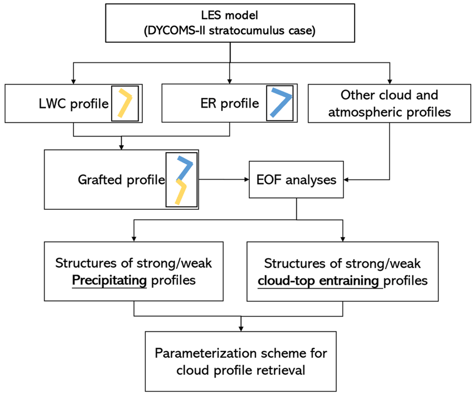
Our analysis is based on two steps described in the following subsections. We first simulate a large ensemble of cloud profiles using an LES model. The design of experiments is illustrated in Fig. 1. We then perform a statistical analysis of those profiles in order to extract the main dominant features of ER and LWC profiles. Those features are later on analyzed in view of the precipitation and entrainment conditions.
2.1 RAMS simulations and cases
Taking advantage of the three-dimensional near-realistic characterization of the stratocumulus layer by an LES (Van Der Dussen et al., 2015), the vertical variability of cloud microphysics is analyzed under different intensities of turbulence and precipitation. We use the LES capability of the Regional Atmospheric Modeling System (RAMS), which is originally developed at Colorado State University, to facilitate research into predominately mesoscale and cloud-scale atmospheric phenomena (Saleeby and Cotton, 2004; Saleeby and Van Den Heever, 2013). The RAMS provides a three-dimensional cloud field simulation with a detailed bulk microphysical scheme, allows interactive grid nesting capabilities, and supports various turbulence closures, shortwave/longwave radiation schemes, and boundary conditions (Pielke et al., 1992). The analysis is based on the nocturnal aircraft measurements obtained during the first research flight (RF01) of the second Dynamics and Chemistry of Marine Stratocumulus (DYCOMS-II) missions, the specifications of which are described by Stevens et al. (2003). This mission records a very homogeneous and extended stratocumulus layer, which is well suited for the study of dry-air entrainment at the cloud top.
The simulations of the DYCOMS-II case are performed with a domain size of km ( bin points) for 3 h. The horizontal resolution is fixed at 100 m, and the vertical bin spacing is 50 m. The initial state of the simulations is based on vertical profiles of potential temperature, moisture, and horizontal winds that were adapted from Stevens et al. (2003). From these initial fields, four additional simulations are carried out by slightly modifying the temperature profiles to check their effects on the stratocumulus field and notably on entrainment rates. In addition, one extra simulation is realized by modifying the humidity profile. In summary, these six simulations are as follows: case 1, “Control”, is the basic simulation with the unmodified fields; case 2, “Control + layer 150 m”, is the same as Control but the temperature inversion is 150 m above that of Control (less brutal than Control), expecting more entrainment; case 3, “Control + layer 300 m”, is the same as Control but the temperature inversion is 300 m above that of Control; case 4, “Control – 4 K”, is the same as Control but with a smaller temperature inversion, expecting more mixing; case 5, “Control + 4 K”, is the same as Control but with a stronger temperature inversion; and case 6, “Extra”, is the same as Control but was initialized using a slightly modified water vapor profile. The vertical gradient of water vapor profile above 850 m in the Extra case is smaller than that in the Control case to entrain more humid air. The potential temperature profiles for these cases are presented in Fig. 2a.
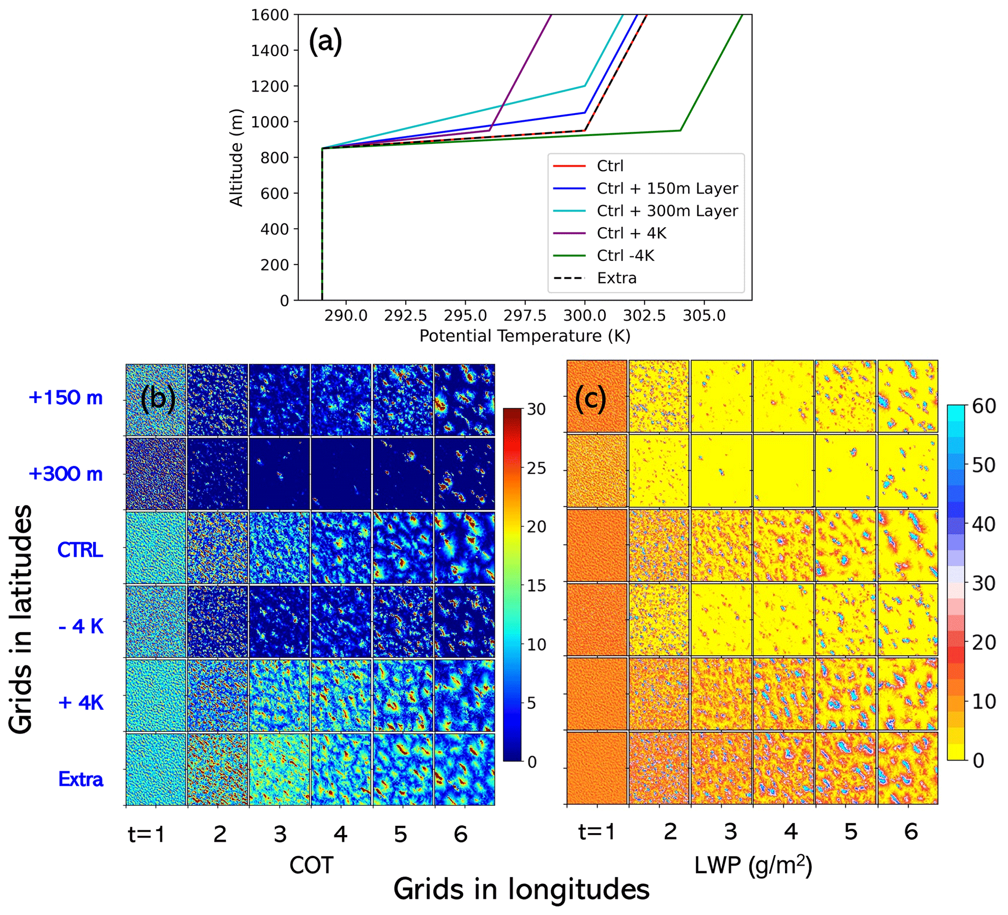
Figure 2Panel (a) the initial potential temperature profiles for the five cases of stratocumulus simulations: “Control”, “Control + layer 150 m”, “Control + layer 300 m”, “Control – 4 K”, “Control + 4 K”, and “Extra” (described in Sect. 2.1); (b) the spatial distribution of cloud optical thickness for the six cases for each 30 min time steps; (c) as in (b) but for the rainwater path, the cloud boundary is determined by the condensation of cloud droplets >20 mg−1.
2.2 EOF analysis
An empirical orthogonal function (EOF) analysis (or equivalently principal component analysis, PCA) is adopted in this study to seek for a limited number of elemental vertical profile variations that explain the maximum amount of variance. Profiles from the RAMS are normalized by the cloud optical thickness so that the cloud top corresponds to 0 and cloud bottom to 1, and, then, normalized profiles are interpolated onto 20 vertical layers. To simultaneously analyze LWC and ER profiles, we grafted every pair of LWC and ER profiles onto one record. Considering that values of ER (µm) and its variance are generally larger than those of LWC (g m−3), direct grafting of the two profiles leads to an overdependence on ER profiles. To balance the weights of two profiles, we multiplied the LWC profiles by a scale factor f that is determined from the ratio of the standard deviation of debiased ER and LWC profiles as follows:
where LWC(i,t) indicates the liquid water content of the ith profile in the tth layer () and ER(i,t) indicates the effective radius likewise. The bar over a quantity indicates the vertical mean. Then, the debiased liquid water content times the scale factor and the debiased effective radius are grafted onto one artificial profile (Eq. 2). Note that whether the ER profile is grafted below or above the LWC profile would not make a difference in the results of the analysis:
Hereby, X(i,j) could be expressed by the first three EOFs:
where w1(i,t) is the weighing factor for EOF1(i,t) (i.e., first dominant EOF) and stands for the average profile of . The ith ER and LWC profiles can be reconstructed by using Eq. (3); the reconstructed LWC profiles will then need to be multiplied by the factor
2.3 Entrainment and precipitation calculation
In this study, we use the entrainment rate (ε) to quantify the inflow of air mass into the cloudy areas. The entrainment rate ε is estimated depending on the relative humidity (RH) according to Eqs. (4) and (5). The parameterization is based on the observational evidence that mid-tropospheric humidity modulates tropical convection. The calculation of ε is also used in the European Centre for Medium-Range Weather Forecasts (ECMWF) convection scheme (De Rooy et al., 2013):
where qsat is the saturation specific humidity at level z and RH is the relative humidity. Stratified cloud entrainment is dependent on cloud depth (De Rooy et al., 2013) and is reduced by an increased RH in the environment. This dependence has a large benefit in the general circulation model of ECMWF. We confirmed the nonlinear negative relation between cloud geometrical thickness (cloud optical thickness as well) and cloud-top entrainment characterized by the value of ε. From Eqs. (2) and (3), it is predictable that smaller RH and larger qsat at level z than at the cloud base will yield larger ε. In this study, cloud profiles with ε at the cloud top being smaller than the 25th percentile are regarded as “weak” cloud-top entrainment cases (WEs), whereas profiles with ε at the cloud top being larger than the 75th percentile are regarded as “strong”' cloud-top entrainment cases (SEs).
Stratocumulus layers are mostly comprised of liquid water and do not produce as much precipitation as deep convective clouds but yield drizzle or light rain (Wood, 2015). We estimate the precipitation from the integrated rainwater content (rainwater path) of each cloud profile that is generated by LES. The histograms in Fig. 3 illustrate the density distributions for the intensities of cloud-top entrainments and precipitation. In the following discussion, we define a profile as strongly precipitating (SP) when the rainwater path exceeds the 75th percentile and weakly precipitating (WP) when the rainwater path remains below the 25th percentile. As we mentioned at the beginning of this paragraph, the SP is characterized merely based on our statistics and is therefore not comparable to strong/heavy precipitation defined in surface meteorological observation.
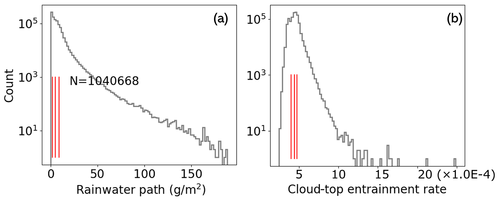
Figure 3Histogram of the counts of the rainwater paths (a) and of the cloud-top entrainment rates (b) in the RAMS cloud profiles; the red vertical lines from left to right indicate the 25th, 50th, and 75th percentiles. A profile is defined as strongly precipitating (SP) when the rainwater path exceeds the 75th percentile and as weakly precipitating (WP) when the rainwater path remains below the 25th percentile. Similarly, a profile is considered and defined as strong cloud-top entrainment (SE) when the entrainment rate at the cloud top exceeds the 75th percentile and as weak cloud-top entrainment (WE) when the entrainment rate at the cloud top is less than the 25th percentile.
3.1 EOFs for the LWC profiles
Adiabatic lifting increases the LWC monotonically with increasing altitude, but other processes such as entrainment of dryer air, mixing process, and precipitation fallout influence the LWC profile. To examine the dominant vertical variation in the LWC profiles among all sampled cloud regimes, we apply the EOF analysis to all instantaneous profiles from six LES runs as described in Sect. 2. The subplot within Fig. 4a shows the first three EOFs, which explain more than 91 % of the total variance. The first and the third EOFs account for 65 % and 8 % of variance, showing that the most significant variation in LWC profiles is monotonic change in LWC from the bottom to the top of clouds. The second EOF accounts for 18 % of variance, indicating that the triangle-shaped polyline is an important structural characteristic besides the monotonic change. EOF2 is indispensable for representing profiles having a positive LWC deviation from the vertical mean LWC in the middle of a cloud together with negative deviations at the cloud top and cloud base. Figure 4a illustrates the 2-D density distribution of the weighting factors of EOF1 and EOF2. The quartile lines in Fig. 4a indicate that the number of outliers is limited, so a close-up view of the density plot is shown in Fig. 4c by removing outliers with weighting factors less than the 1st percentile or larger than the 99th percentile. The highest density of the EOF1 weighting factor is between 0.5 and 4, while that of EOF2 is between 0.5 and 1. As both weighting factors are mostly positive, EOF1 can be interpreted as a representation of vertical growth and EOF2 as a representation of a non-adiabatic process that modifies the profile.
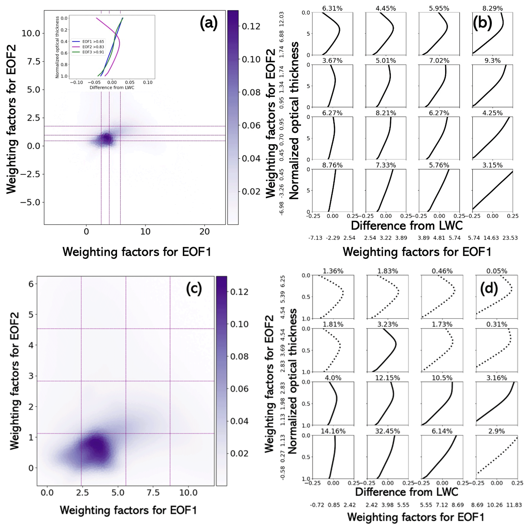
Figure 4(a) Density plot of EOF1 and EOF2 weighting factors for all LWC profiles. The color scale corresponds to the density of the points in percent, and the purple dotted line indicates quartile boundaries along the x and y axes. The inset in (a) illustrates the first three dominant EOFs. They explain the 91 % of variance among all 1 040 668 samples. (b) Cloud LWC profiles reconstructed from EOF1–3 according to quartile bins in (a); the black dotted and solid lines denote the profiles that represent fewer than and more than 3 % of the samples, respectively. (c) Same as (a) but without weighting factors exceed the 99th percentile or less than the 1st percentile and with the purple dotted line indicating the arithmetic mean boundaries. (d) Same as (b), but the reconstruction is based on bins in (c).
Figure 4b and d are the binned reconstruction of LWC profiles according to the binned mean weighting factors in Fig. 4a and c. The fraction of the entire sample that falls into a particular bin is labeled above each diagram. The profiles in bins that represent more than 3 % of the population are marked by solid lines. In either the quartile bin or the arithmetic mean bin, the reconstructed LWC profiles exhibit two main shapes: monotonic increase and triangle-shaped polyline. For the profiles with near-zero EOF2 weighting factors, the reconstructed profiles show a monotonically increasing structure, as we see in the box accounting for 7.33 % in Fig. 4b and the box accounting for 32.45 % in Fig. 4d. On the other hand, the triangle-shaped polyline becomes prevalent when EOF2 weighting factors becomes large, as we see in the box accounting for 8.29 % in Fig. 4b and the box accounting for 12.15 % in Fig. 4d. These triangle-shaped polyline profiles may represent multiple cellular circulations within the cloud that would explain constant LWC values in the upper part of the cloud or may have entrainment that would explain the decreasing LWC in the upper part of the cloud. Therefore, nearly all profiles can be represented either by a monotonic increase or a triangle-shaped polyline with maxima occurring at the turning point close to the middle layer.
3.2 EOFs for the ER profiles
A similar analysis is repeated for the ER profiles to reveal the dominant structure among all the sampled cloud bins. As the LWC and the ER profiles are simultaneously analyzed, the fraction of variance represented by every EOF is identical: 65 % for EOF1, 18 % for EOF2, and 8 % for EOF3. Figure 5a shows the first three EOFs, which together explain 91 % of the variance. The first EOF monotonically increases, the second EOF curves similarly to EOF2 of LWC, and the third EOF monotonically decreases. As the first and third EOFs of LWC are nearly identical, the third EOF serves to adjust the vertical gradient of the ER profile, keeping the LWC profile unchanged. Like the second EOF of LWC, the second EOF of ER can be approximated as a polyline with a turning point corresponding to a maximum positive difference from the average ER at a normalized cloud optical thickness (COT) of 0.4. The density plots in Fig. 5a and c are the same as Fig. 4a and c; they illustrate the 2-D density distribution of first two weighting factors with lines representing either quartile boundaries or arithmetic mean boundaries (with extremes removed).
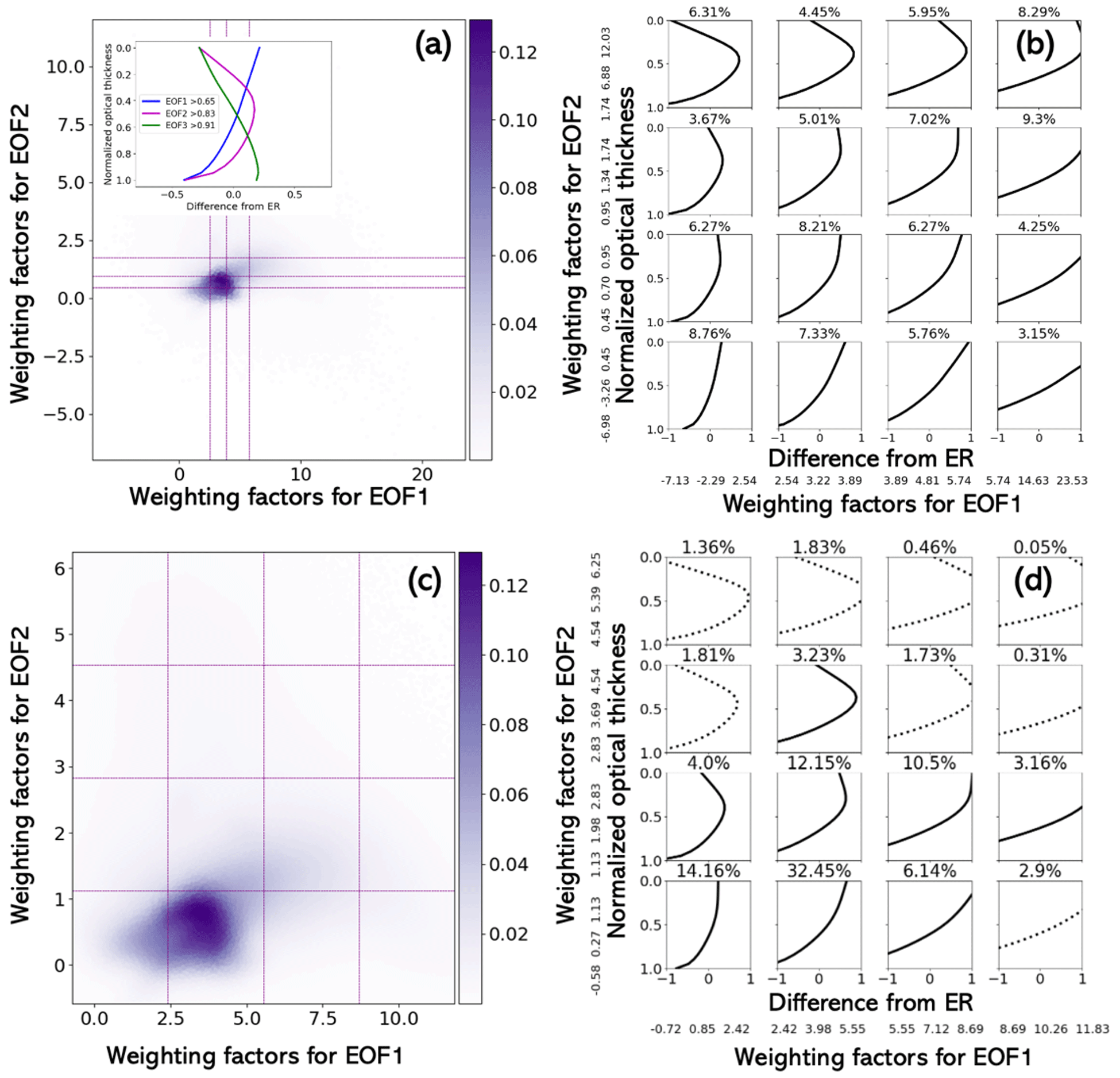
Similar to Fig. 4b and d, the reconstructed cloud ER profiles are shown in Fig. 5b and d. Regardless of bin boundaries, most reconstructed ER profiles are triangle-shaped polylines. Figure 5d indicates that the most dominant profile structure (32.45 %) shows a monotonic ER growth from the cloud base to the cloud top. Others (14.16 %, 12.15 %, 10.5 %) show an explicit increase from the cloud base to the middle of the cloud and then remain unchanged or decrease toward the cloud top. Being consistent with the LWC profiles in Fig. 4, most ER profiles can be represented either by a monotonic increase or a triangle-shaped polyline with maxima occurring at the turning point close to the middle layer.
The variation in weighting factors for dominant EOFs as a function of precipitation and cloud-top entrainment intensities indicates the response of cloud profiles to different cloud entrainment or precipitation conditions. To disentangle the impact of precipitation and cloud-top entrainment, we divide the samples into three-by-three subsets according to three levels of cloud-top entrainment and precipitation. Figure 6 shows the density plot of weighting factors for EOF1 and EOF2 for each subset. In Fig. 6a, vertical and horizontal purple lines in each subplot are first, second, and third quartiles of weighting factors. On the other hand, purple lines in the subplots of Fig. 6b indicate the equidistance division between the 1st percentile and the 99th percentile. Data points with a weighting factor less than the 1st percentile or greater than the 99th percentile are excluded from Fig. 6b.
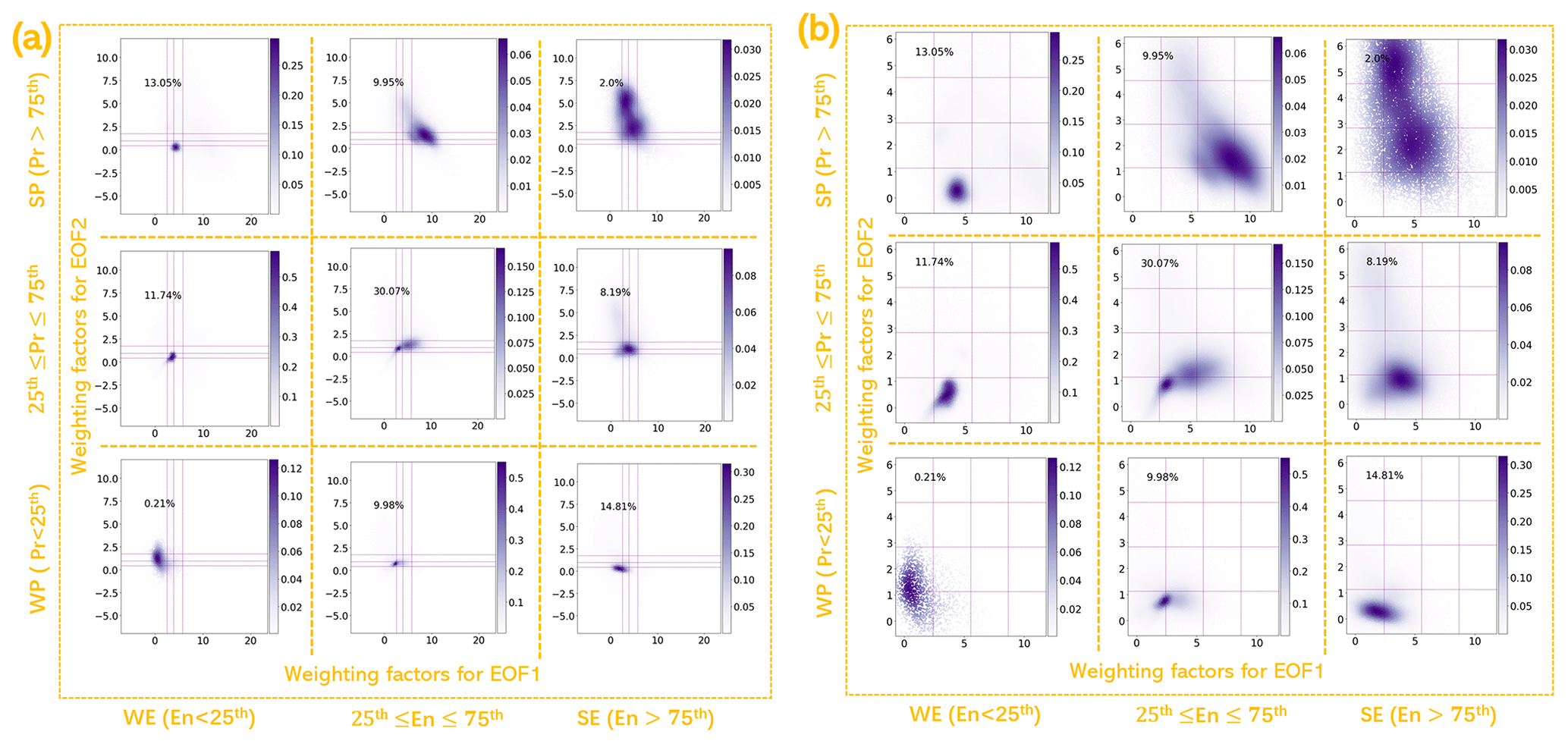
Figure 6The scatterplots of weighting factors for EOF1 and EOF2 for different intensity levels of cloud-top entrainment and precipitation. The weak level, mid-level, and strong level of cloud-top entrainment is characterized by cloud-top entrainment rate below the 25th percentile, in between the 25th and 75th percentiles, and above the 75th percentile. Similarly, three levels of precipitation are characterized by the rainwater path.
Figure 6 shows that the population of points is influenced by both intensities of precipitation and cloud-top entrainment. For example, Fig. 6b demonstrates that the increase in the intensities of cloud-top entrainment for the SP cases (precipitation greater than the 75th percentile) does not only impact the location of the populated points but also disperses the data points. Regardless of the intensities for cloud-top entrainment, the stronger the precipitation is, the larger the weighting factors for EOF1 are. Among WP cloud profiles, it is found that the stronger the cloud-top entrainment is, the smaller the weighting factors for EOF2 are. Among SP cloud profiles, it is found that the stronger the cloud-top entrainment is, the more diversified the profiles are.
In the following subsections, we focus on the fraction of profiles that falls into every box bounded by the purple lines in Fig. 6 to further investigate the variation in profile shape in response to entrainment and precipitation. In addition, we propose a different classification based on the cloud-top slope of the LWC and ER profiles.
4.1 Impact of cloud-top entrainment
To further evaluate the impact of cloud-top entrainment on the LWC and ER profiles, we display the statistics of profiles for WE and SE cases. Figure 7 shows the fractions of profiles that fall into four-by-four bins for WE and SE cases. The analyses are performed with two binning methods: the quartile bin boundaries (Fig. 7a and b) and the arithmetic mean bin boundaries without extremes (as in Fig. 7c and d).
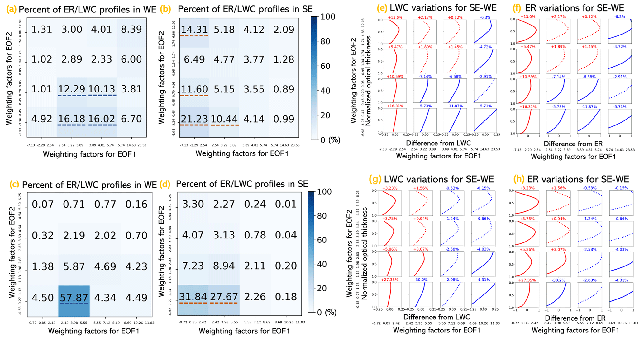
Figure 7(a) The percent of profiles for weak cloud-top entrainment (WE); the bins are characterized by quartile boundaries. (b) Same as (a) but for strong cloud-top entrainment (SE). (c) The percent of profiles for weak cloud-top entrainment (WE); the bins are characterized by arithmetic mean boundaries. (d) Same as (c) but for strong cloud-top entrainment (SE). These boxes that received more than 10 % of the examples are underlined by a dotted blue line for WE cases and by a dotted tangerine one for SE cases. Panels (e) and (f) show the difference between the percent of samples for LWC and ER between SE (b) and WE (a) cases; (g) and (h) show the difference between the percent of samples for LWC and ER between SE (d) and WE (c) cases. In (e)–(h), red color and blue color indicate the increase and decrease in the samples; small variations in percent (within ±3 %) are plotted with a dotted line.
Figure 7 indicates that weighting factors for WE cases are populated in the center bottom boxes (underlined by a dotted blue line in Fig. 7a), whereas those of SE are populated in the boxes in the left column (underlined by a dotted tangerine line in Fig. 7b). This is also indicated by the profiles with solid red lines from Fig. 7e–h. The stronger contribution of EOF1 in representing WE profiles leads to a larger vertical gradient of these profiles compared to SE profiles. For example, the box corresponding to a near-linear profile with a small gradient that accounts for 4.92 % in Fig. 7a receives 21.23 % of samples in Fig. 7b, and the box that accounts for 4.50 % in Fig. 7c receives 31.84 % of samples in Fig. 7d. In addition, WE profiles have smaller EOF2 weights, resulting in less pronounced polyline shapes than SE profiles. Examples can be found in the boxes in the top two rows (in Fig. a–d), corresponding to a more pronounced polyline profile. The examples accounting for, in total, 28.95 % in Fig. 7a receive 42.01 % of samples in Fig. 7b, and the boxes that account for, in total, 6.94 % in Fig. 7c receive 13.84 % of samples in Fig. 7d.
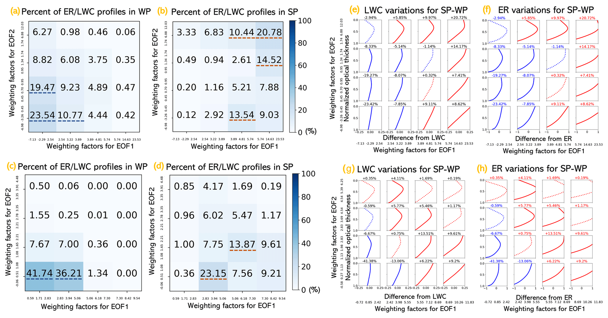
Figure 8(a) The percent of profiles for weak precipitation (WP); the bins are characterized by quartile boundaries. (b) Same as (a) but for strong precipitation (SP). (c) The percent of profiles for weak precipitation (WP); the bins are characterized by arithmetic mean boundaries. (d) Same as (c) but for strong precipitation (SP). The boxes that received more than 10 % of the examples are underlined by a dotted blue line for WE cases and by a dotted tangerine one for SE cases. Panels (e) and (f) show the difference between the percent of samples for LWC and ER between SP (b) and WP (a) cases; (g) and (h) show the difference between the percent of samples for LWC and ER between SP (d) and WP (c) cases. In (e)–(h), red color and blue color indicate the increase and decrease in the samples; small variations in percent (within ±3 %) are plotted with a dotted line.
4.2 Impact of precipitation
As in Sect.4.1, the impact of precipitation is analyzed by the fractions of profiles that fall into 4×4 bins for WP and SP cases (Fig. 8). The analyses are performed with two binning methods: the quartile bin boundaries (Fig. 8a and b) and the arithmetic mean bin boundaries without extremes (as in Fig. 8c and d).
Figure 8 indicates that weighting factors for WP cases are populated in the left bottom boxes in Fig. 8a and c, whereas those of SP are populated in the boxes in the right two columns of Fig. 8b or the center right bottom box (Fig. 8d). The weaker contribution of EOF1 in representing WP profiles leads to the smaller vertical gradient of WP profiles compared to SP profiles. This is also indicated by the profiles with solid red lines from Fig. 8e–h. Examples can be seen from the boxes in the left two columns in Fig. 8a–d. The examples accounting for, in total, 85.16 % in Fig. 8a receive 15.99 % of samples in Fig. 8b, and the boxes that account for, in total, 94.98 % of samples in Fig. 8c receive 44.26 % of samples in Fig. 8d. In addition, WP has smaller EOF2 weights, resulting in less pronounced triangle-shaped polyline profiles than SP cases. Examples can be found in the boxes in the top two rows corresponding to larger EOF2 weights. The examples accounting for, in total, 26.77 % in Fig. 8a receive 59.94 % of samples in Fig. 8b, and the boxes that account for, in total, 2.37 % of samples in Fig. 8c receive 20.52 % of samples in Fig. 8d.
4.3 Implications for the cloud profile retrieval of 3MI
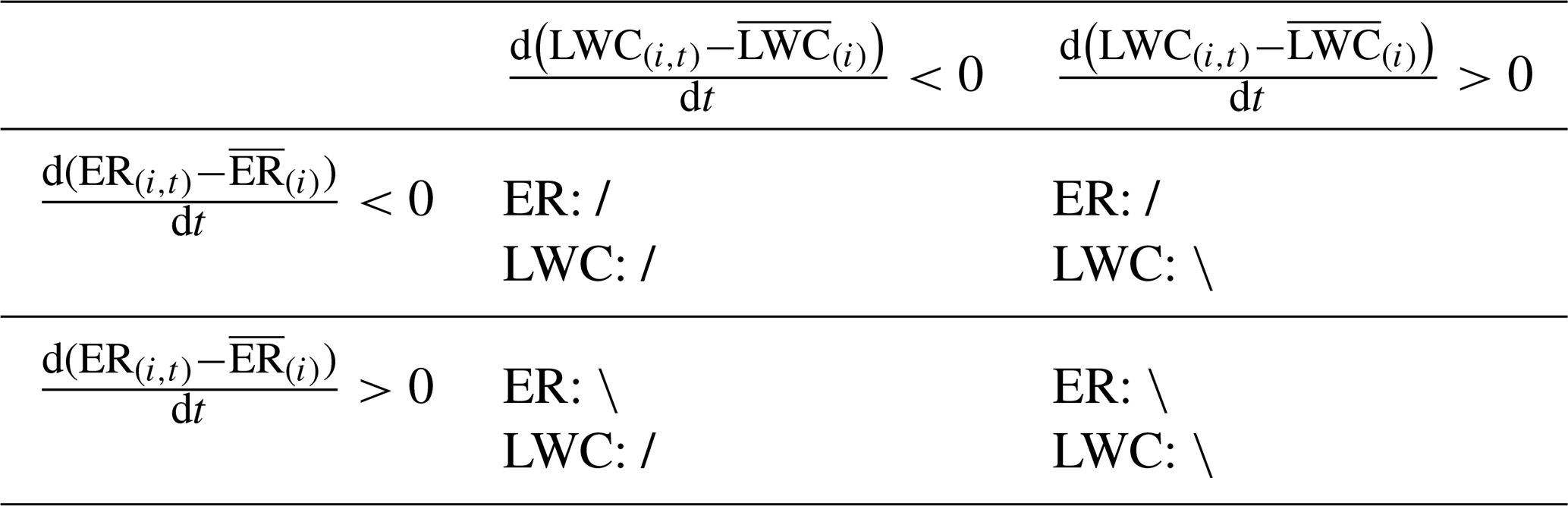
Finally, to summarize the dominant LWC and ER profiles, we divide typical patterns of LWC and ER profiles into four classes. The classification is based merely on the above-turning-point slope () for LWC and ER profiles since the below-turning-point ER and LWC profiles mostly increase with altitude. As the reconstructed LWC and ER detrended profiles are given by the linear combination of three functions as shown in Eq. (3), the above-turning-point slope is also a result of a linear combination of above-turning-point slopes for EOF1–3:
The factors in Eqs. (6) and (7) are visually regressed slopes of the above-turning-point EOF1–3 for LWC and ER, respectively. For both LWC and ER profiles, the slope can be greater or smaller than 0, indicating that LWC or ER decreases or increases toward the cloud top. Hence four categories can be established according to Table 1.
Table 1The criteria to classify four LWC and ER patterns according to the slope of above-turning-point profiles.
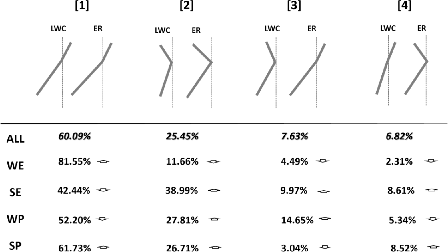
In Table 2, four profile shapes and fractions corresponding to the classification in Table 1 are summarized. The statistics from all cloud profiles as well as four classes (WE, SE, WP, SP) defined by the entrainment and precipitation intensities are presented to evaluate the increase or decrease in a certain profile shape as a consequence of precipitation and cloud-top entrainment. From the turning point to the cloud top, the first pattern corresponds to an increase in both LWC and ER in the upper part of the profiles, the second pattern exhibits a decrease in LWC and ER values in the upper part of the profiles, the third pattern corresponds to a decrease in LWC along with an increase in ER, and the fourth pattern is the opposite of the third pattern. Compared to the statistics of all samples, WE cases strongly increase the fraction of pattern 1 and restrain the other patterns, SE cases decrease pattern 1 and increase patterns 2–4, WP cases reduce the fraction of patterns 1 and 4 while increasing patterns 2 and 3, and SP cases decrease pattern 3 and increase the others.
Table 2The main four LWC–ER patterns that appeared in our analyses and their percentage in terms of the following scenarios: ALL, all cloud profiles; WE, cloud profiles associated with weak cloud-top entrainment; SE, cloud profiles with strong cloud-top entrainment; WP, cloud profiles with weak precipitation; SP, cloud profiles with strong precipitation. The green and red arrows beside the numbers indicate the increase or decrease in the percentage compared with the reference statistics using all samples.
Based on the abovementioned analysis of typical LWC and ER profiles of stratocumulus, we propose a scheme to characterize the ER profiles using simplified triangle-shaped structures. This scheme aims to characterize the LWC and ER for the main patterns summarized in Table 2. Specifically in Fig. 9, the cloud-top ER could be smaller, larger than, or equal to the ER at the turning point. The proposed scheme accepts eight input parameters, namely, the cloud geometrical thickness (zc), the cloud optical thickness (τ), the turning point normalized optical thickness (tm) measured from the cloud top, ER at the cloud base (rb), ER at the cloud top (rt), ER at the turning point (rm), effective variance of gamma size distributions (νe), and the slope (k) of the CDNC profile (N). In this scheme, the ER at different levels (defined by the normalized optical thickness t in Fig. 9) is characterized by the following equations:
where
The power of is selected to maximize the consistency to the existing adiabatic growth theory, in which LWC increases from the cloud base to the cloud top linearly with increasing altitude. Equation (8) is equivalent to this assumption in terms of normalized optical thickness as long as the bulk extinction efficiency is close to 2 and the effective variance of particle size distribution (νe) is constant.
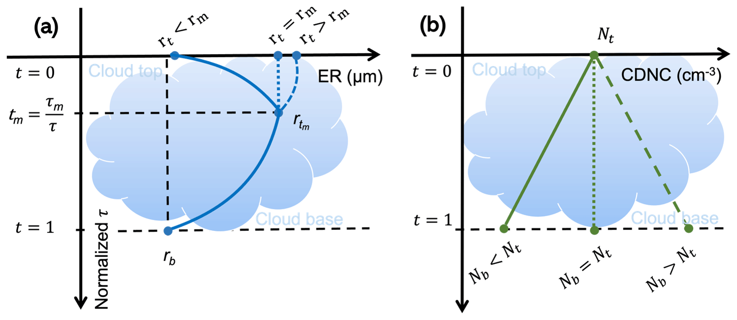
Figure 9(a) Simplified triangle-shaped profiles for the cloud ER and (b) simplified linear profiles for CDNC (N). Both τ or normalized optical thickness (t) axes can be used to define the top (), turning point (, and bottom () of the ER profile. rb, rm, and rt are the effective radii at the cloud base, the turning point, and cloud top, respectively. The N profile is based on a linear assumption with a slope. The stratified values for the ER and LWC profiles are calculated using the parameterization scheme presented in Sect. 5.

Figure 10Four cases of cloud ER, LWC, and CDNC profiles generated by the parametrization scheme.
Furthermore, we add an assumption that the CDNC profile is linear with normalized cloud optical thickness as described by Eq. (10). The CDNC profile can also be a constant value when k=0.
where N0 is the intercept of the regressed linear CDNC profile (i.e., cloud-top CDNC).
With assumed profiles of ER and CDNC in Eqs. (8)–(10), other cloud microphysical parameters can be computed as follows. Since zc is the integration of cloud geometric thickness with respect to cloud normalized optical thickness, we have
where the derivative inside the integral can be derived as
In this derivation, size distributions at every level are assumed to be a gamma distribution with a constant effective variance (νe), but Qext(t) does not need to be approximated as 2. Using the expression obtained in Eq. (12), Eq. (11) can be rewritten as follows:
that is,
All parameters on the right-hand side of Eq. (14) can be obtained from Eq. (9), Mie computation, and assumptions. Then, the number concentration N(t) at any layer can be estimated using Eqs. (10) and (14). The layer-integrated optical thickness (τi), LWC (lwci), and ER (ri) can be computed by Eqs. (15)–(17):
To demonstrate how the scheme represents the cloud profile, four profiles addressing the dominant patterns 1–4 are shown in Fig. 10. For all four profiles, zc is fixed at 0.3 km. Profile (a) shows pattern 1 (Table 1): the scheme captures the monotonic growth of ER and LWC with a turning point at τ=8.0. The CDNC is assumed to be increasing from the cloud base to the cloud top with . Profile (b) shows pattern 2: the dominant feature is that both ER and LWC profiles above the turning point decrease. A constant CDNC profile from the cloud base to the cloud top is assumed. Profile (c) is intended to recreate pattern 3 where the ER profile above the turning point continues to increase while LWC starts to decrease. Profile (d) is the opposite of Profile (c), showing ER decreasing and LWC increasing toward the cloud top. In conclusion, our scheme is capable of representing the dominant patterns of ER and LWC profiles that are summarized in our EOF analysis.
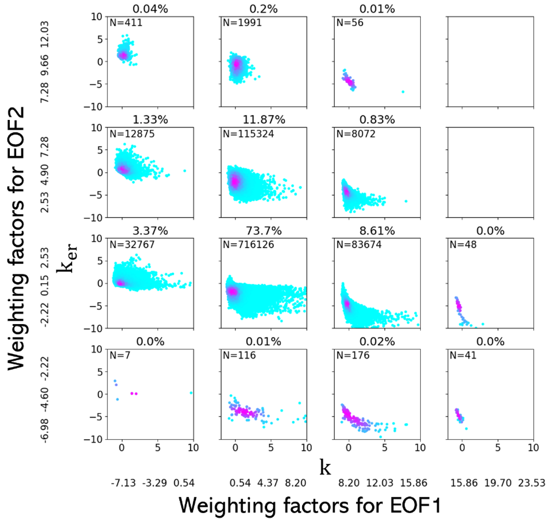
Among the input parameters of the scheme, the slope of CDNC profile (k) is challenging to directly derive from passive measurements. We present some results of preliminary analysis to find relations between k and mean ER, cloud-top ER, and the slope of the ER profile (ker defined by ). Neither the mean ER nor cloud-top ER are found to be closely related to k, but ker and k show a slight correlation. Figure 11 shows the density plots of ker against k. The parameterization of realistic k is reserved for future work, but it appears reasonable that ker and k show some correlation as they are closely related by microphysical processes in clouds.
Characterizing LWC and ER profiles for liquid clouds from passive satellites is challenging and always requires some level of assumptions about the cloud vertical structure to circumvent the limited information content of passive measurements. Establishing physically based constraints to facilitate the characterization of LWC and ER profiles is therefore essential to making progress towards cloud profile retrievals from passive measurements. With this goal in mind, we use simulated cloud profiles of stratocumulus from the DYCOMS-II case to analyze the main structure of LWC and ER profiles. To guarantee consistent LWC and ER structural patterns, we grafted the LWC and ER profiles when performing EOF analyses. We find that >90 % of LWC and ER profiles could be approximated by monotonic increase or triangle-shaped polylines. Besides, LWC and ER profiles have similar concave and convex characteristics and similar locations of turning points. These findings suggest that it is possible to use a reduced number of parameters to describe realistic cloud profiles both in radiative transfer simulation and in actual development of cloud profile retrieval algorithms. From the first three EOFs, monotonically increasing cloud profiles with increasing LWC and ER from the cloud base to the cloud top are found to be the dominant profile variation, but we also observe patterns with LWC and ER nearly constant or decreasing from the turning point to the cloud top. In addition, it is found that the cloud-top entrainment reduces the gradient of LWC and ER profiles, whereas the precipitation increases the gradient of LWC and ER profiles. This can be explained by cloud-top entrainment reducing the ER and LWC at the cloud top where they are usually larger than at the cloud bottom, while the precipitation further reduces the ER and LWC at the cloud bottom by accretion and coalescence where they are usually smaller than at the cloud top.
We noticed four prominent patterns of LWC and ER profiles from the EOF analyses. All these patterns have monotonically increasing LWC and ER profiles in the bottom part of the clouds, while the top part of the profiles may have increasing (pattern 1), decreasing (pattern 2), and contradictory (patterns 3 and 4) LWC and ER variation towards the cloud top. The classification of four prominent patterns of LWC and ER profiles enables us to quantify the pattern variation in cloud profiles by the influence of cloud-top entrainment and precipitation. We found that the dominant patterns are patterns 1 and 2 all the time, and they are more sensitive to cloud-top entrainment than precipitation status: WE (respectively, SE) significantly increases (respectively, decreases) pattern 1 and reduces (respectively, increases) the other patterns, WP reduces patterns 1 and 4 and increases patterns 2 and 3, and SP decreases pattern 3 and increases the others.
Based on the analyses of cloud profiles and assumptions that the turning points of LWC and ER profiles are located at the same position in the normalized COT scale, we propose a parameterization scheme to facilitate the sensitivity studies and retrieval of cloud profiles from passive remote-sensing observations, in particular from the future 3MI. In our scheme, eight parameters are used to describe the vertical variation in cloud optical and microphysical properties. It is shown that the ER and LWC profiles can in most cases be simplified as triangle-shaped profiles with one turning point. Our tests indicate that the scheme can replicate the monotonically increasing, quasi-monotonically increasing, and non-monotonically increasing cloud profiles in terms of the four patterns in our analyses. These results will serve as a basis to develop the retrieval of a liquid cloud vertical profile from the future 3MI observations. It is expected that such retrievals will enable better description of cloud properties, in particular by providing parameters that can be more easily linked to cloud development processes of interest for nowcasting applications.
The RAMS is available at https://vandenheever.atmos.colostate.edu/vdhpage/rams/indexregister.php (Colorado State University, 2023). The simulations of the stratocumulus from RAMS (datasets) are available at https://doi.org/10.5281/zenodo.7578991 (Penide et al., 2023). The codes for the EOF analysis are based on the Scipy library available at https://scipy.org (SciPy, 2023). The implementation of the EOF analysis or the analytical model can be obtained from the authors upon request.
JR and CC outlined the project, HS and SH conceived of the methodology and performed the study, GP performed the simulations, HS composed the article, and all the others revised the article. JR and HL funded, supervised, and encouraged the research.
The contact author has declared that none of the authors has any competing interests.
Publisher's note: Copernicus Publications remains neutral with regard to jurisdictional claims in published maps and institutional affiliations.
The authors are grateful for support from Univ. Lille, CNRS, AIRCAS, and NSFC. We also thank CSU for providing the RAMS model and NCAR for the data for the DYCOMS-II campaign. This work is funded by the National Natural Science Foundation of China (no. 42025504, 42175152) and the Youth Innovation Promotion Association CAS (no. 2021122).
This research has been supported by the National Science Foundation (grant nos. 42025504 and 42175152) and the Youth Innovation Promotion Association CAS (grant no. 2021122).
This paper was edited by Thijs Heus and reviewed by two anonymous referees.
Alexandrov, M. D., Miller, D. J., Rajapakshe, C., Fridlind, A., van Diedenhoven, B., Cairns, B., Ackerman, A. S., and Zhang, Z.: Vertical profiles of droplet size distributions derived from cloud-side observations by the research scanning polarimeter: Tests on simulated data, J. Atmos. Res., 239, 104924, https://doi.org/10.1016/j.atmosres.2020.104924, 2020a.
Alexandrov, M. D., Miller, D. J., Rajapakshe, C., Fridlind, A., van Diedenhoven, B., Cairns, B., Ackerman, A. S., and Zhang, Z.: Vertical profiles of droplet size distributions derived from cloud-side observations by the research scanning polarimeter: Tests on simulated data, Atmos. Res., 239, 104924, https://doi.org/10.1016/j.atmosres.2020.104924, 2020b.
Alexandrov, M. D., Cairns, B., Sinclair, K., Wasilewski, A. P., Ziemba, L., Crosbie, E., Moore, R., Hair, J., Scarino, A. J., and Hu, Y.: Retrievals of cloud droplet size from the research scanning polarimeter data: Validation using in situ measurements, Remote Sens. Environ., 210, 76–95, 2018.
Arabas, S., Pawlowska, H., and Grabowski, W.: Effective radius and droplet spectral width from in-situ aircraft observations in trade-wind cumuli during RICO, Geophys. Res. Lett., 36, L11803, https://doi.org/10.1029/2009GL038257, 2009.
Bréon, F.-M. and Goloub, P.: Cloud droplet effective radius from spaceborne polarization measurements, Geophys. Res. Lett., 25, 1879–1882, https://doi.org/10.1029/98gl01221, 1998.
Breon, F. M. and Doutriaux-Boucher, M.: A comparison of cloud droplet radii measured from space, IEEE T. Geosci. Remote, 43, 1796–1805, https://doi.org/10.1109/TGRS.2005.852838, 2005.
Burns, D., Kollias, P., Tatarevic, A., Battaglia, A., and Tanelli, S.: The performance of the EarthCARE Cloud Profiling Radar in marine stratiform clouds, J. Geophys. Res.-Atmos., 121, 14525–514537, https://doi.org/10.1002/2016JD025090, 2016.
Carey, L. D., Niu, J., Yang, P., Kankiewicz, J. A., Larson, V. E., and Haar, T. H. V.: The Vertical Profile of Liquid and Ice Water Content in Midlatitude Mixed-Phase Altocumulus Clouds, J. Appl. Meteorol. Clim., 47, 2487–2495, https://doi.org/10.1175/2008jamc1885.1, 2008.
Chang, F. L. and Li, Z.: Estimating the vertical variation of cloud droplet effective radius using multispectral near-infrared satellite measurements, J. Geophys. Res.-Atmos., 107, AAC 7-1–AAC 7-12, 2002.
Chang, F. L. and Li, Z.: Retrieving vertical profiles of water-cloud droplet effective radius: Algorithm modification and preliminary application, J. Geophys. Res.-Atmos., 108, 4763, https://doi.org/10.1029/2003JD003906, 2003.
Chen, R., Wood, R., Li, Z., Ferraro, R., and Chang, F.-L.: Studying the vertical variation of cloud droplet effective radius using ship and space-borne remote sensing data, J. Geophys. Res., 113, D00A02, https://doi.org/10.1029/2007jd009596, 2008.
Chen, Y., Chen, G., Cui, C., Zhang, A., Wan, R., Zhou, S., Wang, D., and Fu, Y.: Retrieval of the vertical evolution of the cloud effective radius from the Chinese FY-4 (Feng Yun 4) next-generation geostationary satellites, Atmos. Chem. Phys., 20, 1131–1145, https://doi.org/10.5194/acp-20-1131-2020, 2020.
Colorado State University: Cloud Processes Research Group, https://vandenheever.atmos.colostate.edu/vdhpage/rams/indexregister.php, last access: 22 February 2023.
Cornet, C., C.-Labonnote, L., Waquet, F., Szczap, F., Deaconu, L., Parol, F., Vanbauce, C., Thieuleux, F., and Riédi, J.: Cloud heterogeneity on cloud and aerosol above cloud properties retrieved from simulated total and polarized reflectances, Atmos. Meas. Tech., 11, 3627–3643, https://doi.org/10.5194/amt-11-3627-2018, 2018.
Dadashazar, H., Corral, A. F., Crosbie, E., Dmitrovic, S., Kirschler, S., McCauley, K., Moore, R., Robinson, C., Schlosser, J. S., Shook, M., Thornhill, K. L., Voigt, C., Winstead, E., Ziemba, L., and Sorooshian, A.: Organic enrichment in droplet residual particles relative to out of cloud over the northwestern Atlantic: analysis of airborne ACTIVATE data, Atmos. Chem. Phys., 22, 13897–13913, https://doi.org/10.5194/acp-22-13897-2022, 2022.
Davis, A. B., Merlin, G., Cornet, C., Labonnote, L. C., Riédi, J., Ferlay, N., Dubuisson, P., Min, Q., Yang, Y., and Marshak, A.: Cloud information content in EPIC/DSCOVR's oxygen A- and B-band channels: An optimal estimation approach, J. Quant. Spectrosc. Ra., 216, 6–16, https://doi.org/10.1016/j.jqsrt.2018.05.007, 2018.
de Rooy, W. C., Bechtold, P., Fröhlich, K., Hohenegger, C., Jonker, H., Mironov, D., Pier Siebesma, A., Teixeira, J., and Yano, J.-I.: Entrainment and detrainment in cumulus convection: an overview, Q. J. Roy. Meteor. Soc., 139, 1–19, https://doi.org/10.1002/qj.1959, 2013.
Dong, X. and Mace, G. G.: Profiles of Low-Level Stratus Cloud Microphysics Deduced from Ground-Based Measurements, J. Atmos. Ocean. Tech., 20, 42–53, https://doi.org/10.1175/1520-0426(2003)020<0042:Pollsc>2.0.Co;2, 2003.
Donovan, D. P. and van Lammeren, A. C. A. P.: Cloud effective particle size and water content profile retrievals using combined lidar and radar observations: 1. Theory and examples, J. Geophys. Res.-Atmos., 106, 27425–27448, https://doi.org/10.1029/2001JD900243, 2001.
Fougnie, B., Marbach, T., Lacan, A., Lang, R., Schlüssel, P., Poli, G., Munro, R., and Couto, A. B.: The multi-viewing multi-channel multi-polarisation imager – Overview of the 3MI polarimetric mission for aerosol and cloud characterization, J. Quant. Spectrosc. Ra., 219, 23–32, https://doi.org/10.1016/j.jqsrt.2018.07.008, 2018.
Frisch, A. S., Fairall, C. W., and Snider, J. B.: Measurement of Stratus Cloud and Drizzle Parameters in ASTEX with a Kα-Band Doppler Radar and a Microwave Radiometer, J. Atmos. Sci., 52, 2788–2799, https://doi.org/10.1175/1520-0469(1995)052<2788:Moscad>2.0.Co;2, 1995.
Grosvenor, D. P., Sourdeval, O., Zuidema, P., Ackerman, A., Alexandrov, M. D., Bennartz, R., Boers, R., Cairns, B., Chiu, J. C., Christensen, M., Deneke, H., Diamond, M., Feingold, G., Fridlind, A., Hünerbein, A., Knist, C., Kollias, P., Marshak, A., McCoy, D., Merk, D., Painemal, D., Rausch, J., Rosenfeld, D., Russchenberg, H., Seifert, P., Sinclair, K., Stier, P., van Diedenhoven, B., Wendisch, M., Werner, F., Wood, R., Zhang, Z., and Quaas, J.: Remote Sensing of Droplet Number Concentration in Warm Clouds: A Review of the Current State of Knowledge and Perspectives, Rev. Geophys., 56, 409–453, https://doi.org/10.1029/2017RG000593, 2018a.
Grosvenor, D. P., Sourdeval, O., Zuidema, P., Ackerman, A., Alexandrov, M. D., Bennartz, R., Boers, R., Cairns, B., Chiu, J. C., Christensen, M., Deneke, H., Diamond, M., Feingold, G., Fridlind, A., Hünerbein, A., Knist, C., Kollias, P., Marshak, A., McCoy, D., Merk, D., Painemal, D., Rausch, J., Rosenfeld, D., Russchenberg, H., Seifert, P., Sinclair, K., Stier, P., van Diedenhoven, B., Wendisch, M., Werner, F., Wood, R., Zhang, Z., and Quaas, J.: Remote Sensing of Droplet Number Concentration in Warm Clouds: A Review of the Current State of Knowledge and Perspectives, Rev. Geophys., 56, 409–453, https://doi.org/10.1029/2017RG000593, 2018b.
Illingworth, A. J., Barker, H. W., Beljaars, A., Ceccaldi, M., Chepfer, H., Clerbaux, N., Cole, J., Delanoë, J., Domenech, C., Donovan, D. P., Fukuda, S., Hirakata, M., Hogan, R. J., Huenerbein, A., Kollias, P., Kubota, T., Nakajima, T., Nakajima, T. Y., Nishizawa, T., Ohno, Y., Okamoto, H., Oki, R., Sato, K., Satoh, M., Shephard, M. W., Velázquez-Blázquez, A., Wandinger, U., Wehr, T., and van Zadelhoff, G.-J.: The EarthCARE Satellite: The Next Step Forward in Global Measurements of Clouds, Aerosols, Precipitation, and Radiation, B. Am. Meteorol. Soc., 96, 1311–1332, https://doi.org/10.1175/bams-d-12-00227.1, 2015.
Kokhanovsky, A. and Rozanov, V. V.: Droplet vertical sizing in warm clouds using passive optical measurements from a satellite, Atmos. Meas. Tech., 5, 517–528, https://doi.org/10.5194/amt-5-517-2012, 2012.
Kollias, P., Bharadwaj, N., Widener, K., Jo, I., and Johnson, K.: Scanning ARM Cloud Radars. Part I: Operational Sampling Strategies, J. Atmos. Ocean. Tech., 31, 569–582, https://doi.org/10.1175/jtech-d-13-00044.1, 2014.
Lawson, R. P., Baker, B. A., Schmitt, C. G., and Jensen, T. L.: An overview of microphysical properties of Arctic clouds observed in May and July 1998 during FIRE ACE, J. Geophys. Res., 106, 14989–15014, https://doi.org/10.1029/2000JD900789, 2001.
Letu, H., Yang, K., Nakajima, T. Y., Ishimoto, H., Nagao, T. M., Riedi, J., Baran, A. J., Ma, R., Wang, T., Shang, H., Khatri, P., Chen, L., Shi, C., and Shi, J.: High-resolution retrieval of cloud microphysical properties and surface solar radiation using Himawari-8/AHI next-generation geostationary satellite, Remote Sens. Environ., 239, 111583, https://doi.org/10.1016/j.rse.2019.111583, 2020.
Lhermitte, R. M.: Cloud and precipitation remote sensing at 94 GHz, IEEE T. Geosci. Remote, 26, 207–216, https://doi.org/10.1109/36.3024, 1988.
Lu, C., Niu, S., Liu, Y., and Vogelmann, A. M.: Empirical relationship between entrainment rate and microphysics in cumulus clouds, Geophys. Res. Lett., 40, 2333–2338, https://doi.org/10.1002/grl.50445, 2013.
Lu, C., Liu, Y., Zhang, G. J., Wu, X., Endo, S., Cao, L., Li, Y., and Guo, X.: Improving Parameterization of Entrainment Rate for Shallow Convection with Aircraft Measurements and Large-Eddy Simulation, J. Atmos. Sci., 73, 761–773, https://doi.org/10.1175/jas-d-15-0050.1, 2016.
Lu, M.-L., Conant, W. C., Jonsson, H. H., Varutbangkul, V., Flagan, R. C., and Seinfeld, J. H.: The Marine Stratus/Stratocumulus Experiment (MASE): Aerosol-cloud relationships in marine stratocumulus, J. Geophys. Res.-Atmos., 112, D10209, https://doi.org/10.1029/2006JD007985, 2007.
Lu, M.-L., Sorooshian, A., Jonsson, H. H., Feingold, G., Flagan, R. C., and Seinfeld, J. H.: Marine stratocumulus aerosol-cloud relationships in the MASE-II experiment: Precipitation susceptibility in eastern Pacific marine stratocumulus, J. Geophys. Res.-Atmos., 114, D24203, https://doi.org/10.1029/2009JD012774, 2009.
Mace, G. G. and Sassen, K.: A constrained algorithm for retrieval of stratocumulus cloud properties using solar radiation, microwave radiometer, and millimeter cloud radar data, J. Geophys. Res., 105, 29099–29108, https://doi.org/10.1029/2000JD900403, 2000.
Magaritz-Ronen, L., Pinsky, M., and Khain, A.: Drizzle formation in stratocumulus clouds: effects of turbulent mixing, Atmos. Chem. Phys., 16, 1849–1862, https://doi.org/10.5194/acp-16-1849-2016, 2016.
Marbach, T., Phillips, P., Lacan, A., and Schlüssel, P.: The Multi-Viewing, -Channel, -Polarisation Imager (3MI) of the EUMETSAT Polar System – Second Generation (EPS-SG) dedicated to aerosol characterisation, SPIE Remote Sensing, Proc. SPIE, 8889, 88890I, https://doi.org/10.1117/12.2028221, 2013.
Merlin, G., Riedi, J., Labonnote, L. C., Cornet, C., Davis, A. B., Dubuisson, P., Desmons, M., Ferlay, N., and Parol, F.: Cloud information content analysis of multi-angular measurements in the oxygen A-band: application to 3MI and MSPI, Atmos. Meas. Tech., 9, 4977–4995, https://doi.org/10.5194/amt-9-4977-2016, 2016.
Miles, N. L., Verlinde, J., and Clothiaux, E. E.: Cloud droplet size distributions in low-level stratiform clouds, J. Atmos. Sci., 57, 295–311, https://doi.org/10.1175/1520-0469(2000)057<0295:cdsdil>2.0.co;2, 2000.
Nagao, T. M., Suzuki, K., and Nakajima, T. Y.: Interpretation of Multiwavelength-Retrieved Droplet Effective Radii for Warm Water Clouds in Terms of In-Cloud Vertical Inhomogeneity by Using a Spectral Bin Microphysics Cloud Model, J. Atmos. Sci., 70, 2376–2392, https://doi.org/10.1175/jas-d-12-0225.1, 2013.
Nakajima, T. and King, M. D.: Determination of the optical-thickness and effective particle radius of clouds from reflected solar-radiation measurements, J. Atmos. Sci., 47, 1878–1893, https://doi.org/10.1175/1520-0469(1990)047<1878:dotota>2.0.co;2, 1990.
Nakajima, T. Y., Suzuki, K., and Stephens, G. L.: Droplet Growth in Warm Water Clouds Observed by the A-Train. Part II: A Multisensor View, J. Atmos. Sci., 67, 1897–1907, https://doi.org/10.1175/2010jas3276.1, 2010.
Painemal, D. and Zuidema, P.: Assessment of MODIS cloud effective radius and optical thickness retrievals over the Southeast Pacific with VOCALS-REx in situ measurements, J. Geophys. Res., 116, D24206, https://doi.org/10.1029/2011jd016155, 2011.
Pawlowska, H., Grabowski, W. W., and Brenguier, J.-L.: Observations of the width of cloud droplet spectra in stratocumulus, Geophys. Res. Lett., 33, L19810, https://doi.org/10.1029/2006GL026841, 2006.
Penide, G., Shang, H., Hioki, S., Cornet, C., Letu, H., and Riedi, J.: Simulations of stratocumulus cloud fields using RAMS model, Zenodo [data set], https://doi.org/10.5281/zenodo.7578991, 2023.
Pielke, R. A., Cotton, W. R., Walko, R. L., Tremback, C. J., Lyons, W. A., Grasso, L. D., Nicholls, M. E., Moran, M. D., Wesley, D. A., Lee, T. J., and Copeland, J. H.: A comprehensive meteorological modeling system – RAMS, Meteorol. Atmos. Phys., 49, 69–91, https://doi.org/10.1007/BF01025401, 1992.
Platnick, S.: Vertical photon transport in cloud remote sensing problems, J. Geophys. Res.-Atmos., 105, 22919–22935, https://doi.org/10.1029/2000jd900333, 2000.
Platnick, S.: Approximations for horizontal photon transport in cloud remote sensing problems, J. Quant. Spectrosc. Ra., 68, 75–99, https://doi.org/10.1016/S0022-4073(00)00016-9, 2001.
Platnick, S., Meyer, K. G., King, M. D., Wind, G., Amarasinghe, N., Marchant, B., Arnold, G. T., Zhang, Z., Hubanks, P. A., Holz, R. E., Yang, P., Ridgway, W. L., and Riedi, J.: The MODIS Cloud Optical and Microphysical Products: Collection 6 Updates and Examples From Terra and Aqua, IEEE T. Geosci. Remote, 55, 502–525, https://doi.org/10.1109/TGRS.2016.2610522, 2017.
Rémillard, J., Kollias, P., and Szyrmer, W.: Radar-radiometer retrievals of cloud number concentration and dispersion parameter in nondrizzling marine stratocumulus, Atmos. Meas. Tech., 6, 1817–1828, https://doi.org/10.5194/amt-6-1817-2013, 2013.
Roebeling, R. A., Placidi, S., Donovan, D. P., Russchenberg, H. W. J., and Feijt, A. J.: Validation of liquid cloud property retrievals from SEVIRI using ground-based observations, Geophys. Res. Lett., 35, L05814, https://doi.org/10.1029/2007GL032115, 2008.
Rosenfeld, D. and Lensky, I. M.: Satellite-based insights into precipitation formation processes in continental and maritime convective clouds, B. Am. Meteorol. Soc., 79, 2457–2476, https://doi.org/10.1175/1520-0477(1998)079<2457:sbiipf>2.0.co;2, 1998.
Saito, M., Yang, P., Hu, Y., Liu, X., Loeb, N., Smith Jr., W. L., and Minnis, P.: An Efficient Method for Microphysical Property Retrievals in Vertically Inhomogeneous Marine Water Clouds Using MODIS-CloudSat Measurements, J. Geophys. Res.-Atmos., 124, 2174–2193, https://doi.org/10.1029/2018JD029659, 2019.
Saleeby, S. M. and Cotton, W. R.: A Large-Droplet Mode and Prognostic Number Concentration of Cloud Droplets in the Colorado State University Regional Atmospheric Modeling System (RAMS). Part I: Module Descriptions and Supercell Test Simulations, J. Appl. Meteorol., 43, 182–195, https://doi.org/10.1175/1520-0450(2004)043<0182:Almapn>2.0.Co;2, 2004.
Saleeby, S. M. and van den Heever, S. C.: Developments in the CSU-RAMS Aerosol Model: Emissions, Nucleation, Regeneration, Deposition, and Radiation, J. Appl. Meteorol. Clim., 52, 2601–2622, https://doi.org/10.1175/jamc-d-12-0312.1, 2013.
SciPy: Fundamental algorithms for scientific computing in Python, https://scipy.org, last access: 22 February 2023.
Shang, H., Letu, H., Bréon, F.-M., Riedi, J., Ma, R., Wang, Z., Nakajima, T. Y., Wang, Z., and Chen, L.: An improved algorithm of cloud droplet size distribution from POLDER polarized measurements, Remote Sens. Environ., 228, 61–74, 2019.
Shepherd, J. M., Pierce, H., and Negri, A. J.: Rainfall Modification by Major Urban Areas: Observations from Spaceborne Rain Radar on the TRMM Satellite, J. Appl. Meteorol., 41, 689–701, https://doi.org/10.1175/1520-0450(2002)041<0689:Rmbmua>2.0.Co;2, 2002.
Stephens, G. L., Vane, D. G., Boain, R. J., Mace, G. G., Sassen, K., Wang, Z., Illingworth, A. J., O'connor, E. J., Rossow, W. B., Durden, S. L., Miller, S. D., Austin, R. T., Benedetti, A., and Mitrescu, C.: THE CLOUDSAT MISSION AND THE A-TRAIN: A New Dimension of Space-Based Observations of Clouds and Precipitation, B. Am. Meteorol. Soc., 83, 1771–1790, https://doi.org/10.1175/bams-83-12-1771, 2002.
Stevens, B., Lenschow, D. H., Vali, G., Gerber, H., Bandy, A., Blomquist, B., Brenguier, J.-L., Bretherton, C. S., Burnet, F., Campos, T., Chai, S., Faloona, I., Friesen, D., Haimov, S., Laursen, K., Lilly, D. K., Loehrer, S. M., Malinowski, S. P., Morley, B., Petters, M. D., Rogers, D. C., Russell, L., Savic-Jovcic, V., Snider, J. R., Straub, D., Szumowski, M. J., Takagi, H., Thornton, D. C., Tschudi, M., Twohy, C., Wetzel, M., and van Zanten, M. C.: Dynamics and Chemistry of Marine Stratocumulus – DYCOMS-II, B. Am. Meteorol. Soc., 84, 579–594, 2003.
Suzuki, K., Nakajima, T. Y., and Stephens, G. L.: Particle Growth and Drop Collection Efficiency of Warm Clouds as Inferred from Joint CloudSat and MODIS Observations, J. Atmos. Sci., 67, 3019–3032, https://doi.org/10.1175/2010jas3463.1, 2010.
van der Dussen, J. J., de Roode, S. R., Dal Gesso, S., and Siebesma, A. P.: An LES model study of the influence of the free tropospheric thermodynamic conditions on the stratocumulus response to a climate perturbation, J. Adv. Model. Earth Sy., 7, 670–691, https://doi.org/10.1002/2014MS000380, 2015.
Wang, J., Daum, P. H., Yum, S. S., Liu, Y., Senum, G. I., Lu, M.-L., Seinfeld, J. H., and Jonsson, H.: Observations of marine stratocumulus microphysics and implications for processes controlling droplet spectra: Results from the Marine Stratus/Stratocumulus Experiment, J. Geophys. Res., 114, https://doi.org/10.1029/2008jd011035, 2009.
Wood, R.: CLOUDS AND FOG | Stratus and Stratocumulus, in: Encyclopedia of Atmospheric Sciences (Second Edition), edited by: North, G. R., Pyle, J., and Zhang, F., Academic Press, Oxford, 196–200, https://doi.org/10.1016/B978-0-12-382225-3.00396-0, 2015.
Wu, P., Dong, X., Xi, B., Tian, J., and Ward, D. M.: Profiles of MBL Cloud and Drizzle Microphysical Properties Retrieved From Ground-Based Observations and Validated by Aircraft In Situ Measurements Over the Azores, J. Geophys. Res.-Atmos., 125, e2019JD032205, https://doi.org/10.1029/2019JD032205, 2020.
Xu, X., Lu, C., Liu, Y., Luo, S., Zhou, X., Endo, S., Zhu, L., and Wang, Y.: Influences of an entrainment–mixing parameterization on numerical simulations of cumulus and stratocumulus clouds, Atmos. Chem. Phys., 22, 5459–5475, https://doi.org/10.5194/acp-22-5459-2022, 2022.
Zhang, Z., Ackerman, A. S., Feingold, G., Platnick, S., Pincus, R., and Xue, H.: Effects of cloud horizontal inhomogeneity and drizzle on remote sensing of cloud droplet effective radius: Case studies based on large-eddy simulations, J. Geophys. Res.-Atmos., 117, D19208, https://doi.org/10.1029/2012jd017655, 2012.
Zhao, C., Qiu, Y., Dong, X., Wang, Z., Peng, Y., Li, B., Wu, Z., and Wang, Y.: Negative Aerosol-Cloud re Relationship From Aircraft Observations Over Hebei, China, Earth Space Sci., 5, 19–29, https://doi.org/10.1002/2017EA000346, 2018.
- Abstract
- Introduction
- Data and methods
- Typical structures of LWC and ER profiles for stratocumulus
- Impact of cloud-top entrainment or precipitation on the LWC and ER profiles
- Cloud parameterization scheme for cloud vertical profiles
- Conclusions
- Data availability
- Author contributions
- Competing interests
- Disclaimer
- Acknowledgements
- Financial support
- Review statement
- References