the Creative Commons Attribution 4.0 License.
the Creative Commons Attribution 4.0 License.
 | 01 Feb 2023
Natural marine cloud brightening in the Southern Ocean
Sally Benson
Ruhi Humphries
Peter M. Gombert
Elizabeth Sterner
The number of cloud droplets per unit volume (Nd) is a fundamentally important property of marine boundary layer (MBL) liquid clouds that, at constant liquid water path, exerts considerable controls on albedo. Past work has shown that regional Nd has a direct correlation to marine primary productivity (PP) because of the role of seasonally varying, biogenically derived precursor gases in modulating secondary aerosol properties. These linkages are thought to be observable over the high-latitude oceans, where strong seasonal variability in aerosol and meteorology covary in mostly pristine environments. Here, we examine Nd variability derived from 5 years of MODIS Level 2-derived cloud properties in a broad region of the summer eastern Southern Ocean and adjacent marginal seas. We demonstrate latitudinal, longitudinal and temporal gradients in Nd that are strongly correlated with the passage of air masses over high-PP waters that are mostly concentrated along the Antarctic Shelf poleward of 60∘ S. We find that the albedo of MBL clouds in the latitudes south of 60∘ S is significantly higher than similar liquid water path (LWP) clouds north of this latitude.
- Article
(1711 KB) - Full-text XML
- BibTeX
- EndNote


The cloud and precipitation properties of the Southern Ocean (SO) have received considerable attention since Trenberth and Fasullo (2010) identified a high bias in surface-absorbed solar energy there (McFarquhar et al., 2021). This bias has been traced to erroneously small marine boundary layer (MBL) cloud cover in simulations of the Southern Ocean climate (Bodas-Salcedo, et al., 2016; Naud et al., 2016). The actual SO cloud climatology and associated albedo are dominated by geometrically thin MBL clouds (Mace, 2010; Mace et al., 2021a). Because the predominant shallow boundary layer clouds rarely precipitate (Huang et al., 2016), they are sensitive to cloud condensation nuclei (CCN) concentrations (Twohy and Anderson, 2008; Painemal et al., 2017).
In the SO, the CCN seasonal cycle (Ayers and Gras, 1991; Vallina et al., 2006; Gras and Keywood, 2017) is reflected in basin-wide cloud property variations (Krüger and Graßl, 2011). McCoy et al. (2015) and Mace and Avey (2017) also found that MODIS- and A-Train-derived cloud properties over the SO demonstrate a similar seasonal cycle in cloud droplet number concentration (Nd) to CCN. The basin-wide variability in CCN and cloud albedo has been shown to be correlated with marine primary productivity (PP – defined as the net organic matter, mostly produced by phytoplankton, that is suspended in the ocean; Vallina et al., 2006; Krüger and Graßl, 2011; McCoy et al., 2015). McCoy et al. (2020) argue that the SO can be viewed as an analog of the preindustrial Earth. Given the large natural seasonal variability in CCN and clouds, the SO is a natural laboratory to understand the processes that contribute to simulated aerosol-related indirect forcing variability in climate models (Carslaw et al., 2013).
CCN and cloud droplet Nd in the SO are higher in summer, when significant latitudinal gradients have been documented in the SO Australasian sector (Humphries et al., 2021). Using a time-of-flight aerosol chemical speciation monitor (ACSM) and ion concentrations from filter samples, Humphries et al. (2021) analyzed the covariance of aerosol chemistry, CCN at 0.5 % supersaturation and condensation nuclei (CN) larger than 10 nm collected aboard Australian research vessels during the 2018 Austral summer (McFarquhar et al., 2021). While sulfates were a major compositional component of aerosol at all latitudes during summer, these compounds were in higher fractional abundance poleward of 65∘ S, where overall CCN numbers were higher by ∼ 50 %. Chloride derived from sea salt was dominant in the region equatorward of 65∘ S but was mostly absent south of 65∘ S. The ratio of CCN to CN at 0.5 % supersaturation increased considerably south of 65∘ S, suggesting unique aerosol chemical processes compared to the open ocean. Humphries et al. (2021) also discuss how this compositional boundary in aerosol chemistry is often very distinct in the East Antarctic waters between 60 and 65∘ S. Following Humphries et al. (2021) we refer to this belt as the Atmosphere Compositional Front of Antarctica (ACFA). Humphries et al. (2021) conclude that aerosol, newly condensed from gas-phase sulfur species such as from the oxidation of dimethyl sulfide (DMS), is an important component of high-latitude CCN. These products of phytoplankton physiology are released into the atmosphere from the highly productive waters from ∼ 60∘ S to the Antarctic – a region well known for a vast marine food web (Deppeler and Davidson, 2017; Behrenfeld et al., 2017).
Mace et al. (2021b) derived Nd and other cloud microphysical properties from nonprecipitating stratocumulus clouds using shipborne remote sensing data. They found that stratiform clouds poleward of the ACFA had significantly higher Nd than equatorward. One particular case took place when the icebreaker Aurora Australis was at the Davis Antarctic station just east of Prydz Bay (∼ 77∘ E) between 1 and 5 January 2018 and featured nearly continuous high-Nd clouds (>150 cm−3) occurring in a southerly flow passing over the ship that had trajectories from the Antarctic continent. Similarly, Twohy et al. (2021) report that the highest concentrations of aerosol composed primarily of non-sea-salt sulfates in the free troposphere north of 60∘ S observed from research aircraft in summer 2018 had occurred in air masses that had originated recently from over the Antarctic continent. See also Shaw (1988) for an early examination of the role of biogenic sulfate in modulating summertime aerosol along coastal Antarctica. Shaw (2007) expand on this idea, as do Korhonen et al. (2008).
See Appendix A for methods and definitions. Approximately 40 000 1∘ latitude × 2∘ longitude MBL cloud scenes per month meet our criteria for liquid-phase nonprecipitating clouds in the analysis domain. This number varies by ∼ 25 % in a seasonal cycle that is due mostly to our solar zenith angle criteria. A seasonal cycle is evident in the monthly averaged cloud properties. LWP and re have seasonal minima in the months of December and January. Due to an dependence, Nd is of opposite phase to re and correlated with it at −0.93. The seasonal variability in LWP (re) is on the order of 7 % (4 %) and is small in comparison to Nd (∼ 25 %). τ and re are derived from the visible and near-infrared reflectances with the MODIS Level 2 retrieval algorithm (Nakajima and King, 1990). LWP is then calculated from
which is derived in Stephens (1978). It is reasonable to consider whether seasonal variations in Nd, perhaps linked to CCN, might be associated with variability in LWP. We find that LWP decreases as Nd increases, with a correlation coefficient in the monthly means of −0.60.
In 4 of the 5 years, we see by inspection of Fig. 1 that chl-a leads changes in Nd by approximately 1 month. The correlation coefficient of Nd and chl-a increases from 0.27 to 0.60 when Nd is lagged from 0 to 1 month in the Fig. 1 time series, although this result should be interpreted with caution given the break between February and November in the time series. These results are broadly like those presented by McCoy et al. (2015) and Mace and Avey (2017). McCoy et al. (2015) link Nd variations to PP using regression analysis of MODIS-derived Nd against a biogeochemical parameterization of biogenic sulfate and organic mass fraction (see also Lana et al., 2012).
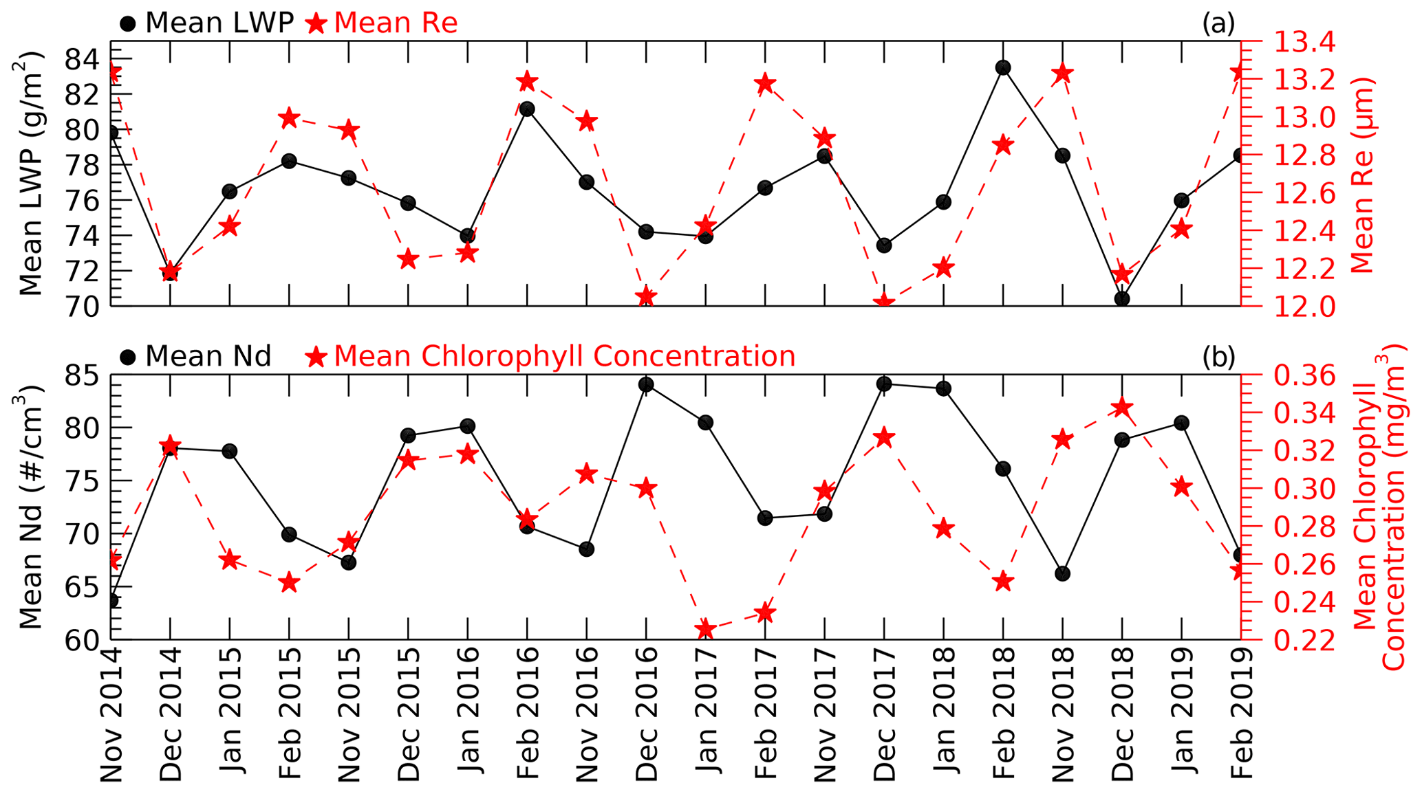
Figure 1Monthly averaged cloud properties and chlorophyll-a (chl-a; Hu et al., 2019) derived from MODIS data over the analysis domain. (a) LWP (black dots and solid line) and effective radius (Re, red star and dashed line). (b) Nd (black dots and solid line) and chl-a concentration (red star and dashed line).
We find a broad distribution of scene-averaged Nd (Fig. 2a) with median, lower and upper quartile values of 66, 42 and 101 cm−3, respectively. Henceforth, we focus our analysis on the groups of scenes that are less than and greater than the upper and lower quartiles. The high- and low-Nd scenes have distinct latitudinal occurrence distributions (Fig. 2b), with low-Nd scenes peaking broadly at 48∘ S, while the high-Nd scenes demonstrate a modal occurrence near 64∘ S. Overall, the Nd gradient implied by Fig. 2 is correlated with the latitudinal distribution of imager-derived chl-a (i.e., Deppeler and Davidson, 2017). The seasonally averaged Nd gradient is also discussed in McCoy et al. (2020). Differentiating seasonally varying properties north and south of the ACFA (not shown), we find a clear differentiation in re and Nd with smaller re south of the ACFA (mean re∼11 µm, Nd∼100) compared to north (mean re∼ 13 µm, Nd∼67 cm−3). LWP is slightly larger by ∼ 7 % south of the ACFA. Both regions have a distinct seasonal cycle in cloud properties, as shown in Fig. 1, although the southern latitudes have larger interannual variability, likely owing to variations in annual sea ice extent and melt. The LWP distribution of the high-Nd quartile is significantly shifted to lower values compared to the low-Nd quartile LWP distribution (Fig. 2c). This finding is in accordance with the observational and theoretical work presented in Glassmeier et al. (2021), who argue that closed-cell stratocumulus that dominate the clouds examined here have increased entrainment drying under higher-Nd conditions. Figure 2c and d illustrate that even though the high-Nd-quartile scenes tend to have lower LWP, their solar albedo (A) tends to be significantly higher than the low-Nd-quartile scenes, illustrating the influence of cloud microphysics on the radiative forcing of these clouds.
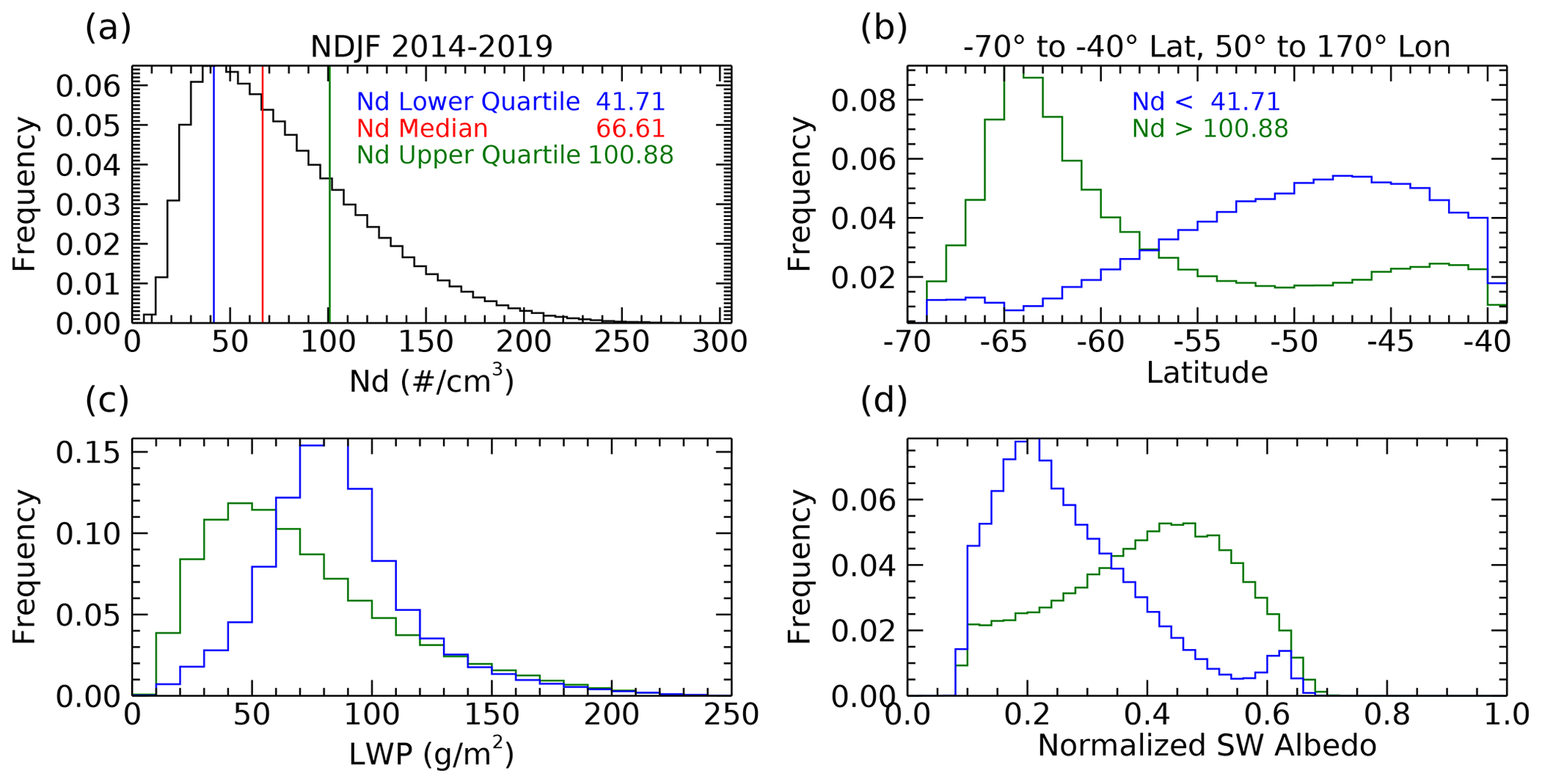
Figure 2(a) Nd frequency distribution from the cloud scenes in the analysis domain during the 5 years of summer months analyzed. Colored vertical lines are defined in the inset. (b) The latitudinal distributions of the cloud scenes that compose the high- and low-Nd quartiles. (c) the distributions of LWP for the high- and low-Nd quartiles, (d) the distribution of normalized CERES solar albedo of the high- and low-Nd quartiles. The normalization procedure is described in the Appendix. The colors of the histograms in panels (b), (c) and (d) are as described in the inset of panel (a).
The high-Nd scenes occur predominantly poleward of the ACFA (Fig. 3). Interestingly we find that the latitudinal gradient weakens slightly west of 90∘ E, with a broad region of higher Nd occurrence in the vicinity of the Kerguelen Rise, where PP is higher (Cavagna et al., 2015). Establishing causality between regions of high PP and cloud properties is challenging (i.e., Meskhidze and Nenes, 2006; Miller and Yuter, 2008). While we find seasonal associations over broad regions here, the chain of causality between phytoplankton and clouds is not immediate or even necessarily direct because the chemical processes take time to evolve and can move along chemical pathways that have divergent outcomes (Woodhouse et al., 2013). To increase cloud Nd, new CCN must be formed. Formation of new CCN can occur when sulfur compounds emitted from the ocean surface nucleate after oxidation in the presence of sunlight. This process of new particle formation occurs in the absence of other aerosol and often requires mixing of the gaseous compounds from the boundary layer into the low-aerosol free troposphere, where the newly formed aerosol can be transported widely (Shaw, 2007; Korhonen et al., 2008). Other pathways are possible such as deposition of sulfate compounds onto primary sea salt particles that modify the chemical properties of existing CCN rather than nucleating new CCN (Fossum et al., 2020) or even removal of sulfur compounds from the gas phase via aqueous-phase oxidation in clouds (Woodhouse et al., 2013).
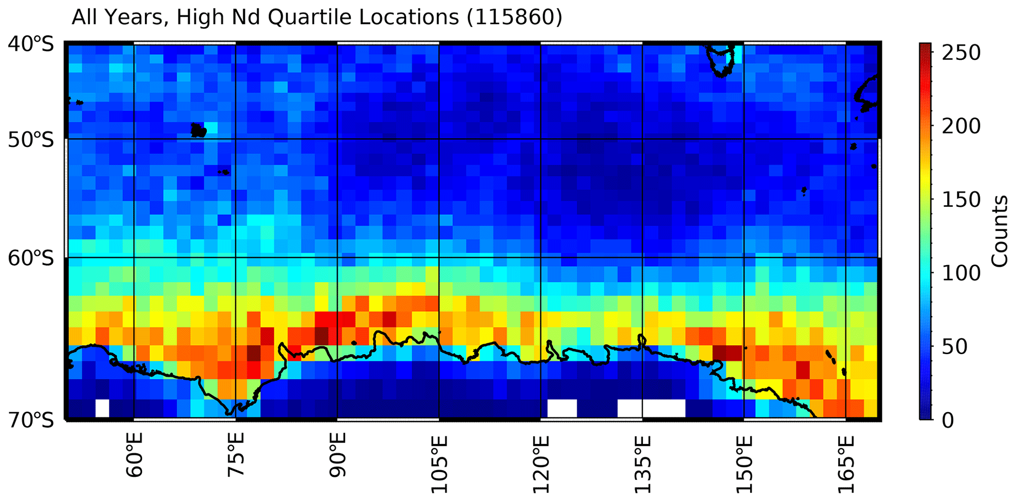
Figure 3Geographic distribution of the high-Nd-quartile cloud scenes. The number in parentheses shows the total of number cloud scenes from the 5-year summer data set.
Given the foregoing discussion, it seems reasonable that an air mass that is producing clouds with certain features could be interacting with an aerosol population that has evolved over periods of days (Brechtel et al., 1998). In addition, natural cloud processes such as collision and coalescence of drops tend to cause Nd to decrease, while precipitation efficiently scavenges CCN, thereby lowering CCN concentration and even modifying their composition and size through aqueous processing (Hoppel et al., 1986). With larger re north of the ACFA, the collision–coalescence process is likely more active (Freud and Rosenfeld, 2012) and could explain the latitudinal difference in adiabaticity (see “Methods” section) found in in situ data. For instance, Kang et al. (2022) analyzed data collected from Macquarie Island (54.6∘ S, 158.9∘ E) and found that not only were most clouds drizzling but also that precipitation as light as 0.01 mm h−1 could reduce Nd by ∼ 50 %. Therefore, a cloud field should be considered to be the product of both local dynamics and thermodynamics primarily with modulation by a local population of CCN. To examine the role of air mass history, we calculate the 5 d back trajectories using the Hybrid Single-Particle Lagrangian Integrated Trajectory (HYSPLIT; Stein et al., 2015) model using the Global Data Assimilation System (GDAS; Kanamitsu, 1989) as input. The parcel's endpoint is the central latitude and longitude of the cloud scene, and the location and model output are stored hourly.
South of the ACFA, the histories of the populations tend to be statistically different (Fig. 4). The low-Nd clouds are more likely to be observed in air masses that have trajectories that originated in the open-ocean region to the north of the ACFA. High-Nd scenes rarely evolve in air masses that originate in the open ocean to the north of the ACFA. The likelihood is that an air mass that has produced a high-Nd cloud scene south of the ACFA latitude has spent most of the previous 5 d over latitudes south of the ACFA. North of the ACFA, the latitude distributions during the months of November and February (not shown) are essentially identical for the high- and low-Nd quartiles. However, for December and January, we find that the high-Nd clouds observed north of the ACFA have an increased likelihood of trajectories emanating from south of the ACFA during the 5 d prior to the MODIS observation.
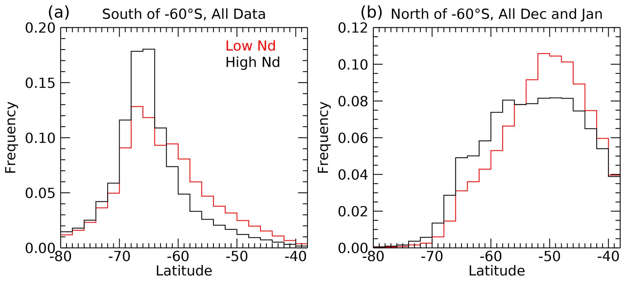
Figure 4Distributions of the latitudes crossed by the 5 d back trajectories for the low- (red) and high-Nd (black) cloud scenes.
Using MODIS Level 2 cloud property retrievals and the technique developed in Grosvenor et al. (2018; hereafter G18) to estimate Nd, we examine the latitudinal and seasonal cycles of nonprecipitating liquid-phase clouds in the Australasian sector of the summertime Southern Ocean. The re and Nd have distinctive differences north and south of the ACFA but demonstrate similar seasonal cycles. We infer that the spatial and temporal variability in cloud Nd, and re is at least partially a function of the geographic and temporal variability in CCN, which, in turn, is related to the seasonality of primary sources such as sea salt and the latitudinal variability in marine PP. The highest-Nd clouds tend to be overwhelmingly found along the East Antarctic coastal waters south of the ACFA.
Because aerosol precursor gases like DMS often require trajectories through the free troposphere to nucleate new particles that then take time to reach CCN sizes (Korohonen et al., 2008; Shaw, 2007), we examine the back trajectories of the air masses observed with high and low Nd south of the ACFA and find significant differences. Low-Nd cloud scenes are more likely to have arrived south of the ACFA from northerly trajectories that would have transported low-CCN air dominated by sea salt. The high-Nd cloud scenes are more likely to have trajectories that have remained adjacent to or had passed over the Antarctic continent. North of the ACFA, while the trajectory statistics for the high- and low-Nd quartiles in November and February are nearly identical, during December and January the high-Nd cloud scenes tend to have an increased likelihood of arriving north of the ACFA from southerly trajectories, suggesting that high-CCN air masses are being transported northward, especially during December and January.
Given that the main difference between the source regions north and south of the ACFA is the magnitude of the marine PP, and given previous analyses of CCN compositional sensitivity to marine biological factors (e.g., Humphries et al., 2021; Vallina et al., 2006; Lana et al., 2012; McCoy et al., 2015), we conclude that the biological source of sulfate precursor gases and the slackening of surface winds with latitude during summer play a dominating role in controlling the latitudinal gradients in the properties of weakly precipitating MBL cloud fields over the Southern Ocean. Figure 5 summarizes our findings by presenting composite seasonal cycles of MBL cloud scenes north and south of 60∘ S. The LWPs in both latitudinal bands go through a weak seasonal cycle. The significant contrast in optical depth between the northern and southern bands is, we infer, mostly caused by the latitudinal contrast in Nd. Based on available evidence, we conclude that the differences in re in MODIS retrievals are causally linked to oceanic PP gradients that drive CCN, and thereby Nd, to be higher over the southern region. This sensitivity, in turn, plays a significant role in modulating the regional albedo (A) and, thereby, influences the input of sunlight to the surface ocean. We note that the seasonal cycle in A is different between the northern and southern latitude domains (a topic for future work); however, A of the southern domain is always higher than that of the northern domain. However, we should be careful not to overstate this case. Cloud processes that consume Nd and modify CCN (i.e., precipitation and cloud processing) also play a role in modulating cloud Nd and therefore regional A (Kang et al., 2022; McCoy et al., 2020). The air mass history and source region, while apparently important, are among many factors involved.
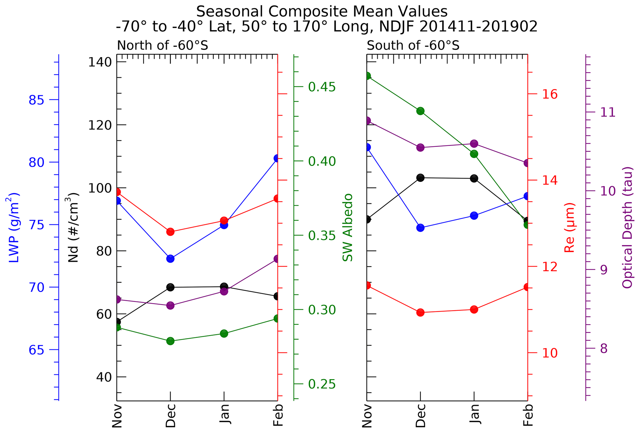
Figure 5Composite seasonal cycle of cloud properties. Each data point is comprised of the monthly mean of cloud scenes in the analysis domain compiled from November 2014–February 2019. The effective radius (Re, red curve) and the optical depth (solid purple curve) are taken directly from MODIS Level 2 retrievals. The liquid water path (LWP, blue curve) and cloud droplet number (Nd, black curve) are derived as described in the text. The solar (SW) albedo (green curve) is derived from CERES data and normalized to a solar zenith angle of 45∘ as described in the Appendix.
Since the magnitude of PP is significantly lower north of the ACFA throughout the summer season, a similar seasonal cycle in Nd and re suggests that CCN derived from DMS oxidation of precursor gases emitted primarily from Antarctic coastal waters perhaps seed much of the rest of the Southern Ocean with biogenic sulfate aerosol, as observed in recent airborne observations (Twohy et al., 2021). The northerly transport of these high-sulfate air masses out of the Antarctic coastal waters (Fig. 4b) and southerly transport of low-sulfate air masses into the Antarctic coastal region near the surface (Fig. 4a) have been reported by Humphries et al. (2016, 2021) and Shaw (1988) and observed in the free troposphere with recent research aircraft measurements (Twohy et al., 2021).
Our ability to identify natural marine cloud brightening (Latham et al., 2008) due to aerosol–cloud coupling is a direct result of the absence of other anthropogenic and continental influences in the pristine SO. As argued by McCoy et al. (2020), it seems clear that in several important ways, the Southern Ocean is the last vestige of the preindustrial atmosphere allowing us to constrain processes that remain important to our understanding of the global climate (Carslaw et al., 2013).
We use MODIS-imager-derived Level 2 retrievals (Platnick et al., 2015) of effective radius (re) and optical depth (τ) from five summer periods (2014–2019) collected between the latitudes of 45 and 76∘ S and longitudes of 40 and 170∘ E to focus roughly on where the ships and aircraft sampled in summer 2017–2018. We calculate Nd using the method derived and evaluated in G18:
where ρw is the density of liquid water (1 g cm−3), fad is an adiabaticity assumption, cw is the vertical derivative of the adiabatic liquid water content, Qext is the extinction efficiency that is typically assumed to be 2 for cloud droplets, and κ is the cubed ratio of re to rv. As noted by G18, Nd depends on , which implies that the sensitivity of the rate of change in Nd to retrieved re goes as the exponent. Any biases in re then would significantly bias Nd. G18 provide a thorough evaluation of the sources of uncertainty in Nd due to assumptions of adiabaticity, scene heterogeneity, etc. and conclude that Nd derived using Eq. 1 applied to MODIS cloud retrievals has an overall uncertainty of ∼ 80 %.
The most uncertain quantity in the assumptions used in Eq. A1 is fad since the cloud vertical structure is not constrained by MODIS measurements. Using cloud thickness from ship-based cloud radar and lidar along with retrieved LWP from collocated microwave radiometer measurements (Mace et al., 2021b), we estimate the value of fad in nonprecipitating stratocumulus observed during the summer of 2018 (McFarquhar et al., 2021). We find that the mean and standard deviation of fad north of the ACFA are 0.66 and 0.48, respectively. South of the ACFA, the mean and standard deviation of fad are 0.93 and 0.60, respectively. For the calculations of Nd in Eq. A1, we use a constant value for fad of 0.8. Nd is proportional to the square root of fad; therefore, , and a fractional variation in fad on the order of 0.5 would imply an uncertainty in Nd of 0.25. Furthermore, we expect in regions with fad higher (lower) than 0.8 that the Nd would be biased low (high). As we show, the regions with higher Nd tend to be in the south, and the regions with lower Nd tend to be in the north, counter to these expected biases. Additionally in this study, we examine differences in spatially averaged Nd that are greater than a factor of 2. These results imply that bias and random error due to uncertainty in fad are unlikely to significantly influence the qualitative findings of this study.
Another source of systematic bias could be from the quantity κ that can be shown to be a function of the variance of the droplet size distribution and is assumed to be a constant at 0.7. G18 discuss this issue in some detail and conclude that there may be systematic biases on the order of 12 % that could be a function of Nd under pristine conditions. While this quantity can be investigated with data collected in situ, no such data exist in stratocumulus clouds south of the ACFA. Therefore, we recognize a potential source of bias due to κ that is likely much smaller than the systematic latitudinal differences we find.
Given the uncertainties in Nd at the pixel level, we implement a filtering and averaging scheme to focus on liquid-phase, weakly precipitating cloud scenes. We define a scene as a 1∘ latitude × 2∘ longitude domain where pixels are reported in the MODIS Level 2 data to be of liquid phase. We assume that clouds are weakly precipitating clouds if the cloud liquid water path (LWP) <300 g m−2. We require that the sensor and solar zenith angles (θ) at that pixel are less than 30 and 60∘, respectively. The maximum θ requirement is motivated by the findings of Grosvenor and Wood (2014), who find that systematic errors in MODIS retrievals increase significantly for θ>60∘. The θ requirement causes us to focus on the months from November through February. We require at least 1000 1 km resolution pixels with these characteristics to exist within a scene (typical number >10 000). In addition, we require that no more than 10 % of the pixels have a cloud top temperature less than −20 ∘C to ensure the absence of ice-phase hydrometeors. Cloud properties within a scene are averaged.
Collocated cloud albedos (A) of the cloud scenes are analyzed. A is derived from the Clouds and the Earth's Radiant Energy System (CERES) Energy Balanced and Filled (EBAF) version 4.0 (Loeb et al., 2018) data collected using instruments on board Aqua and Terra. The albedo is derived by dividing the upwelling shortwave flux at the top of the atmosphere (TOA) by the downwelling shortwave flux at TOA. Because A has a solar zenith angle (θ) dependence (Minnis et al. 1998), we normalize all albedo values to θ=45∘ (approximately the mean value of θ for the analysis domain and months analyzed) with an empirical method using theoretically calculated A () as a function of latitude presented in Minnis et al. (1998, their Fig. 7). The normalization is implemented by first approximating the latitudinal dependence of A for various cloud optical depths (τ) using the following regression equation: , where μ0=cos θ. approximates the variation in A with latitude within ∼ 15 % at τ=8. The fit decreases in accuracy at higher and lower τ, increasing to an uncertainty of ∼ 30 % for τ=2 and τ=32 (these values of τ (2, 8, 32) are those presented in Fig. 7 of Minnis et al., 1998). The averaged τ of the cloud scenes in our analysis is approximately between 9 and 11 (Fig. 5), so we expect that is typically a reasonable approximation of A. The normalization of all A to θ=45∘ is accomplished by multiplying the CERES A by the ratio , where τ is from the MODIS cloud scene. The magnitude of the ratio applied to the data ranges from 0.85 at higher latitudes to 1.2 at lower latitudes, with an average near 1.
Computer code for this study including all analysis code and graphic generation code is written in the IDL language and is available at https://doi.org/10.7278/S50d-bpx8-gmtt (Mace et al., 2022).
All data used in this study are available in public archives. MODIS cloud products can be found for Terra and Aqua at https://doi.org/10.5067/TERRA/MODIS/L3M/CHL/2018 (NASA Goddard Space Flight Center et al., 2018) and https://doi.org/10.5067/MODIS/MYD06_L2.006 (Platnick et al., 2015). Chlorophyll-a data are obtained from MODIS Level 3 standard mapped image products available at https://doi.org/10.5067/AQUA/MODIS/L3M/CHL/2022 (NASA Goddard Space Flight Center et al., 2022). CERES data are available at https://doi.org/10.5067/AQUA/CERES/SSF-FM3_L2.004A (NASA Langley Atmospheric Science Data Center DAAC, 2014). MODIS geolocation data can be obtained at https://doi.org/10.5067/MODIS/MOD03.061 (MODIS Characterization Support Team, 2017). GDAS data are obtained from ftp://ftp.arl.noaa.gov/pub/archives/gdas (National Centers for Environmental Prediction, 2022).
GGM led the overall conception, data analysis of the study and interpretation of the results. SB was responsible for implementing data analysis code and generation of figures. RH provided background on aerosol chemistry and processes. PMG and ES assisted GGM in the study design and implementation.
The contact author has declared that none of the authors has any competing interests.
Publisher’s note: Copernicus Publications remains neutral with regard to jurisdictional claims in published maps and institutional affiliations.
This research has been supported by the Science Mission Directorate (grant no. 80NSSC21k1969) and the DOE ASR (grant nos. DE-SC00222001 and DESC0018995).
This paper was edited by Barbara Ervens and Martina Krämer and reviewed by two anonymous referees.
Ayers, G. and Gras, J.: Seasonal relationship between cloud condensation nuclei and aerosol methanesulphonate in marine air, Nature, 353, 834–835, https://doi.org/10.1038/353834a0, 1991.
Behrenfeld, M. J., Hu, Y., O'Malley, R. T., Boss, E. S., Hostetler, C. A., Siegel, D. A., Sarmiento, J. L., Schulien, J., Hair, J. W., Lu, X., Rodier, S., and Scarino, A. J.: Annual boom–bust cycles of polar phytoplankton biomass revealed by space-based lidar, Nat. Geosci., 10, 118–122, https://doi.org/10.1038/ngeo2861, 2017.
Bodas-Salcedo, A., Hill, P. G., Furtado, K., Williams, K. D., Field, P. R., Manners, J. C., Hyder, P., and Kato, S.: Large Contribution of Supercooled Liquid Clouds to the Solar Radiation Budget of the Southern Ocean, J. Climate, 29, 4213–4228, https://doi.org/10.1175/jcli-d-15-0564.1, 2016.
Brechtel, F. J., Kreidenweis, S. M., and Swan, H. B.: Air mass characteristics, aerosol particle number concentrations, and number size distributions at Macquarie Island during the First Aerosol Characterization Experiment (ACE 1), J. Geophys. Res.-Atmos., 103, 16351–16367, https://doi.org/10.1029/97jd03014, 1998.
Carslaw, K. S., Lee, L. A., Reddington, C. L., Pringle, K. J., Rap, A., Forster, P. M., Mann, G. W., Spracklen, D. V., Woodhouse, M. T., Regayre, L. A., and Pierce, J. R.: Large contribution of natural aerosols to uncertainty in indirect forcing, Nature, 503, 67–71, https://doi.org/10.1038/nature12674, 2013.
Cavagna, A. J., Fripiat, F., Elskens, M., Mangion, P., Chirurgien, L., Closset, I., Lasbleiz, M., Florez-Leiva, L., Cardinal, D., Leblanc, K., Fernandez, C., Lefèvre, D., Oriol, L., Blain, S., Quéguiner, B., and Dehairs, F.: Production regime and associated N cycling in the vicinity of Kerguelen Island, Southern Ocean, Biogeosciences, 12, 6515–6528, https://doi.org/10.5194/bg-12-6515-2015, 2015.
Deppeler, S. L. and Davidson, A. T.: Southern Ocean Phytoplankton in a Changing Climate, Frontiers in Marine Science, 4, 2296–7745, https://doi.org/10.3389/fmars.2017.00040, 2017.
Fossum, K. N., Ovadnevaite, J., Ceburnis, D., Preißler, J., Snider, J. R., Huang, R.-J., Zuend, A., and O'Dowd, C.: Sea-spray regulates sulfate cloud droplet activation over oceans, npj Climate and Atmospheric Science, 3, 14, https://doi.org/10.1038/s41612-020-0116-2, 2020.
Freud, E. and Rosenfeld, D.: Linear relation between convective cloud drop number concentration and depth for rain initiation, J. Geophys. Res., 117, D02207, https://doi.org/10.1029/2011JD016457, 2012.
Glassmeier, F., Hoffmann, F., Johnson, J. S., Yamaguchi, T., Carslaw, K. S., and Feingold, G.: Aerosol-cloud-climate cooling overestimated by ship-track data, Science, 371, 485–489, https://doi.org/10.1126/science.abd3980, 2021.
Gras, J. L. and Keywood, M.: Cloud condensation nuclei over the Southern Ocean: wind dependence and seasonal cycles, Atmos. Chem. Phys., 17, 4419–4432, https://doi.org/10.5194/acp-17-4419-2017, 2017.
Grosvenor, D. P. and Wood, R.: The effect of solar zenith angle on MODIS cloud optical and microphysical retrievals within marine liquid water clouds, Atmos. Chem. Phys., 14, 7291–7321, https://doi.org/10.5194/acp-14-7291-2014, 2014.
Grosvenor, D. P., Sourdeval, O., Zuidema, P., Ackerman, A., Alexandrov, M. D., Bennartz, R., Boers, R., Cairns, B., Chiu, J. C., Christensen, M., Deneke, H., Diamond, M., Feingold, G., Fridlind, A., Hünerbein, A., Knist, C., Kollias, P., Marshak, A., McCoy, D., and Quaas, J.: Remote Sensing of Droplet Number Concentration in Warm Clouds: A Review of the Current State of Knowledge and Perspectives, Rev. Geophys., 56, 409–453, https://doi.org/10.1029/2017rg000593, 2018.
Hoppel, W. A., Frick, G. M., and Larson, R. E.: Effect of nonprecipitating clouds on the aerosol size distribution in the marine boundary layer, Geophys. Res. Lett., 13, 125–128, https://doi.org/10.1029/gl013i002p00125, 1986.
Hu, C., Feng, L., Lee, Z., Franz, B. A., Bailey, S. W., Werdell, P. J., and Proctor, C. W.: Improving satellite global chlorophyll a data products through algorithm refinement and data recovery, J. Geophys. Res.-Oceans, 124, 1524–1543, https://doi.org/10.1029/2019JC014941, 2019.
Huang, Y., Siems, S. T., Manton, M. J., Rosenfeld, D., Marchand, R., McFarquhar, G. M., and Protat, A.: What is the Role of Sea Surface Temperature in Modulating Cloud and Precipitation Properties over the Southern Ocean?, J. Climate, 29, 7453–7476, https://doi.org/10.1175/jcli-d-15-0768.1, 2016.
Humphries, R. S., Klekociuk, A. R., Schofield, R., Keywood, M., Ward, J., and Wilson, S. R.: Unexpectedly high ultrafine aerosol concentrations above East Antarctic sea ice, Atmos. Chem. Phys., 16, 2185–2206, https://doi.org/10.5194/acp-16-2185-2016, 2016.
Humphries, R. S., Keywood, M. D., Gribben, S., McRobert, I. M., Ward, J. P., Selleck, P., Taylor, S., Harnwell, J., Flynn, C., Kulkarni, G. R., Mace, G. G., Protat, A., Alexander, S. P., and McFarquhar, G.: Southern Ocean latitudinal gradients of cloud condensation nuclei, Atmos. Chem. Phys., 21, 12757–12782, https://doi.org/10.5194/acp-21-12757-2021, 2021.
Kang, L., Marchand, R. R., Wood, R., and McCoy, I. L.: Coalescence Scavenging Drives Droplet Number Concentration in Southern Ocean Low Clouds, J. Geophys. Res., 49, e2022GL097819, https://doi.org/10.1029/2022GL097819, 2022.
Kanamitsu, M.: Description of the NMC Global Data Assimilation and Forecast System, Weather Forecast., 4, 335–342, https://doi.org/10.1175/1520-0434(1989)004<0335:dotngd>2.0.co;2, 1989.
Korhonen, H., Carslaw, K. S., Spracklen, D. V., Mann, G. W., and Woodhouse, M. T.: Influence of oceanic dimethyl sulfide emissions on cloud condensation nuclei concentrations and seasonality over the remote Southern Hemisphere oceans: A global model study, J. Geophys. Res., 113, D15204, https://doi.org/10.1029/2007JD009718, 2008.
Krüger, O. and Graßl, H.: Southern Ocean phytoplankton increases cloud albedo and reduces precipitation, Geophys. Res. Lett., 38, L08809, https://doi.org/10.1029/2011gl047116, 2011.
Lana, A., Simó, R., Vallina, S. M., and Dachs, J.: Potential for a biogenic influence on cloud microphysics over the ocean: a correlation study with satellite-derived data, Atmos. Chem. Phys., 12, 7977–7993, https://doi.org/10.5194/acp-12-7977-2012, 2012.
Latham, J., Rasch, P., Chen, C.-C., Kettles, L., Gadian, A., Gettelman, A., Morrison, H., Bower, K., and Choularton, T.: Global temperature stabilization via controlled albedo enhancement of low-level maritime clouds, Philos. T. R. Soc. A, 366, 3969–3987, https://doi.org/10.1098/rsta.2008.0137, 2008.
Loeb, N. G., Doelling, D. R., Wang, H., Su, W., Nguyen, C., Corbett, J. G., Liang, L., Mitrescu, C., Rose, F. G., and Kato, S.: Clouds and the Earth’s Radiant Energy System (CERES) Energy Balanced and Filled (EBAF) Top-of-Atmosphere (TOA) Edition-4.0 Data Product, J. Climate, 31, 895–918, https://doi.org/10.1175/JCLI-D-17-0208.1, 2018.
Mace, G. G.: Cloud properties and radiative forcing over the maritime storm tracks of the Southern Ocean and North Atlantic derived from A-train, J. Geophys. Res.-Atmos., 115, D10201, https://doi.org/10.1029/2009jd012517, 2010.
Mace, G. G. and Avey, S.: Seasonal variability of warm boundary layer cloud and precipitation properties in the Southern Ocean as diagnosed from A-Train Data, J. Geophys. Res.-Atmos., 122, 1015–1032, https://doi.org/10.1002/2016jd025348, 2017.
Mace, G. G., Protat, A., and Benson, S.: Mixed-phase clouds over the Southern Ocean as observed from satellite and surface based lidar and radar, J. Geophys. Res.-Atmos., 126, e2021JD034569, https://doi.org/10.1029/2021jd034569, 2021a.
Mace, G. G., Protat, A., Humphries, R. S., Alexander, S. P., McRobert, I. M., Ward, J., Selleck, P., Keywood, M., and McFarquhar, G. M.: Southern Ocean cloud properties derived from CAPRICORN and MARCUS data, J. Geophys. Res.-Atmos., 126, e2020JD033368, https://doi.org/10.1029/2020jd033368, 2021b.
Mace, G. G., Benson, S., Humphries, R., Gombert P. M., and Sterner, E.: IDL Code for: “Natural marine cloud brightening in the Southern Ocean.” Atmospheric Chemistry and Physics, The Hive: University of Utah Research Data Repository [code], https://doi.org/10.7278/S50d-bpx8-gmtt, 2022.
McCoy, D. T., Burrows, S. M., Wood, R., Grosvenor, D. P., Elliott, S. M., Ma, P.-L., Rasch, P. J., and Hartmann, D. L.: Natural aerosols explain seasonal and spatial patterns of Southern Ocean cloud albedo, Science Advances, 1, e1500157, https://doi.org/10.1126/sciadv.1500157, 2015.
McCoy, I. L., McCoy, D. T., Wood, R., Regayre, L., Watson-Parris, D., Grosvenor, D. P., Mulcahy, J. P., Hu, Y., Bender, F. A.-M., Field, P. R., Carslaw, K. S., and Gordon, H.: The hemispheric contrast in cloud microphysical properties constrains aerosol forcing, P. Natl. Acad. Sci. USA, 117, 18998–19006, https://doi.org/10.1073/pnas.1922502117, 2020.
McFarquhar, G. M., Bretherton, C. S., Marchand, R., Protat, A., DeMott, P. J., Alexander, S. P., Roberts, G. C., Twohy, C. H., Toohey, D., Siems, S., Huang, Y., Wood, R., Rauber, R. M., Lasher-Trapp, S., Jensen, J., Stith, J. L., Mace, J., Um, J., Järvinen, E., Schnaiter, M., Gettelman, A., Sanchez, K. J., McCluskey, C. S., Russell, L. M., McCoy, I. L., Atlas, R. L., Bardeen, C. G., Moore, K. A., Hill, T. C. J., Humphries, R. S., Keywood, M. D., Ristovski, Z., Cravigan, L., Schofield, R., Fairall, C., Mallet, M. D., Kreidenweis, S. M., Rainwater, B., D’Alessandro, J., Wang, Y., Wu, W., Saliba, G., Levin, E. J. T., Ding, S., Lang, F., Truong, S. C. H., Wolff, C., Haggerty, J., Harvey, M. J., Klekociuk, A. R., and McDonald, A.: Observations of Clouds, Aerosols, Precipitation, and Surface Radiation over the Southern Ocean: An Overview of CAPRICORN, MARCUS, MICRE, and SOCRATES, B. Am. Meteorol. Soc., 102, E894–E928, https://doi.org/10.1175/bams-d-20-0132.1, 2021.
Meskhidze, N. and Nenes, A.: Phytoplankton and Cloudiness in the Southern Ocean, Science, 314, 1419–1423, https://doi.org/10.1126/science.1131779, 2006.
Miller, M. A. and Yuter, S. E.: Lack of correlation between chlorophyll-a and cloud droplet effective radius in shallow marine clouds, Geophys. Res. Lett., 35, L13807, https://doi.org/10.1029/2008gl034354, 2008.
Minnis, P., Garber, D.P., Young, D. F., Arduini, R. F., and Takano, Y.: Parameterizations of Reflectance and Effective Emittance for Satellite Remote Sensing of Cloud Properties, J. Atmos. Sci., 55, 3313–3339, https://doi.org/10.1175/1520-0469(1998)055<3313:PORAEE>2.0.CO;2, 1998.
MODIS Characterization Support Team (MCST): MODIS Geolocation Fields Product, NASA MODIS Adaptive Processing System, Goddard Space Flight Center, USA [data set], https://doi.org/10.5067/MODIS/MOD03.061, 2017.
Nakajima, T. and King, M. D.: Determination of the Optical Thickness and Effective Particle Radius of Clouds from Reflected Solar Radiation Measurements. Part I: Theory, J. Atmos. Sci., 47, 1878–1893, https://doi.org/10.1175/1520-0469(1990)047<1878:DOTOTA>2.0.CO;2, 1990.
NASA Goddard Space Flight Center, Ocean Ecology Laboratory, and Ocean Biology Processing Group: Moderate-resolution Imaging Spectroradiometer (MODIS) Terra Chlorophyll Data; 2018 Reprocessing, NASA OB.DAAC, Greenbelt, MD, USA [data set], https://doi.org/10.5067/TERRA/MODIS/L3M/CHL/2018, 2018.
NASA Goddard Space Flight Center, Ocean Ecology Laboratory, and Ocean Biology Processing Group: Moderate-resolution Imaging Spectroradiometer (MODIS) Aqua Chlorophyll Data; 2022 Reprocessing, NASA OB.DAAC, Greenbelt, MD, USA [data set], https://doi.org/10.5067/AQUA/MODIS/L3M/CHL/2022, 2022.
NASA Langley Atmospheric Science Data Center DAAC: CERES Single Scanner Footprint (SSF) TOA/Surface Fluxes, Clouds and Aerosols Edition 4A CER_SSF_Aqua-FM3-MODIS_Edition4A_400403.2014013104.hdf NASA/LARC/SD/ASDC, CERES Single Scanner Footprint (SSF) TOA/Surface Fluxes, Clouds and Aerosols Aqua-FM3 Edition4A [Data set], https://doi.org/10.5067/AQUA/CERES/SSF-FM3_L2.004A, 2014.
National Centers for Environmental Prediction (NCEP): Global Data Assimilation System (GDAS), NOAA Air Resources Laboratory (ARL) [data set], ftp://ftp.arl.noaa.gov/pub/archives/gdas1, last access: 1 August 2022.
Naud, C. M., Booth, J. F., and Del Genio, A. D.: The Relationship between Boundary Layer Stability and Cloud Cover in the Post-Cold-Frontal Region, J. Climate, 29, 8129–8149, https://doi.org/10.1175/jcli-d-15-0700.1, 2016.
Painemal, D., Chiu, J.-Y. C., Minnis, P., Yost, C., Zhou, X., Cadeddu, M., Eloranta, E., Lewis, E. R., Ferrare, R., and Kollias, P.: Aerosol and cloud microphysics covariability in the northeast Pacific boundary layer estimated with ship-based and satellite remote sensing observations, J. Geophys. Res.-Atmos., 122, 2403–2418, https://doi.org/10.1002/2016JD025771, 2017.
Platnick, S., Ackerman, S. A., King, M. D., Meyer, K., Menzel, W. P., Holz, R. E., Baum, B. A., and Yang, P.: MODIS Atmosphere L2 Cloud Product (06_L2), NASA MODIS Adaptive Processing System, Goddard Space Flight Center, USA [data set], https://doi.org/10.5067/MODIS/MYD06_L2.006, 2015.
Shaw, G. E.: Antarctic aerosols: A review, Rev. Geophys., 26, 89–112, https://doi.org/10.1029/RG026i001p00089,1988.
Shaw, G. E.: Do biologically produced aerosols really modulate climate?, Environ. Chem., 4, 382–383, https://doi.org/10.1071/EN07073, 2007.
Stein, A. F., Draxler, R. R., Rolph, G. D., Stunder, B. J., Cohen, M. D., and Ngan, F.: NOAA's HYSPLIT Atmospheric Transport and Dispersion Modeling System, B. Am. Meteorol. Soc., 96, 2059–2077, https://doi.org/10.1175/bams-d-14-00110.1, 2015.
Stephens, G. L.: Radiation Profiles in Extended Water Clouds. II: Parameterization Schemes, J. Atmos. Sci., 35, 2123–2132, https://doi.org/10.1175/1520-0469(1978)035<2123:RPIEWC>2.0.CO;2, 1978.
Trenberth, K. E. and Fasullo, J. T.: Simulation of Present-Day and Twenty-First-Century Energy Budgets of the Southern Oceans, J. Climate, 23, 440–454, https://doi.org/10.1175/2009jcli3152.1, 2010.
Twohy, C. H., and Anderson, J. R: Droplet nuclei in non-precipitating clouds: composition and size matter, Environ. Res. Lett., 3, 045002, https://doi.org/10.1088/1748-9326/3/4/045002, 2008.
Twohy, C. H., DeMott, P. J., Russell, L. M., Toohey, D. W., Rainwater, B., Geiss, R., Sanchez, K. J., Lewis, S., Roberts, G. C., Humphries, R. S., McCluskey, C. S., Moore, K. A., Selleck, P. W., Keywood, M. D., Ward, J. P., and McRobert, I. M.: Cloud-nucleating particles over the Southern Ocean in a changing climate, Earth's Future, 9, e2020EF001673, https://doi.org/10.1029/2020ef001673, 2021.
Vallina, S. M., Simó, R., and Gassó, S.: What controls CCN seasonality in the Southern Ocean? A statistical analysis based on satellite-derived chlorophyll and CCN and model-estimated OH radical and rainfall, Global Biogeochem. Cy., 20, GB1014, https://doi.org/10.1029/2005gb002597, 2006.
Woodhouse, M. T., Mann, G. W., Carslaw, K. S., and Boucher, O.: Sensitivity of cloud condensation nuclei to regional changes in dimethyl-sulphide emissions, Atmos. Chem. Phys., 13, 2723–2733, https://doi.org/10.5194/acp-13-2723-2013, 2013.