Trends in polar ozone loss since 1989: potential sign of recovery in the Arctic ozone column

Ozone depletion over the polar regions is monitored each year by satellite- and ground-based instruments. In this study, the vortex-averaged ozone loss over the last 3 decades is evaluated for both polar regions using the passive ozone tracer of the chemical transport model TOMCAT/SLIMCAT and total ozone observations from Système d'Analyse par Observation Zénithale (SAOZ) ground-based instruments and Multi-Sensor Reanalysis (MSR2). The passive-tracer method allows us to determine the evolution of the daily rate of column ozone destruction and the magnitude of the cumulative column loss at the end of the winter. Three metrics are used in trend analyses that aim to assess the ozone recovery rate over both polar regions: (1) the maximum ozone loss at the end of the winter, (2) the onset day of ozone loss at a specific threshold, and (3) the ozone loss residuals computed from the differences between annual ozone loss and ozone loss values regressed with respect to sunlit volume of polar stratospheric clouds (VPSCs). This latter metric is based on linear and parabolic regressions for ozone loss in the Northern Hemisphere and Southern Hemisphere, respectively. In the Antarctic, metrics 1 and 3 yield trends of −2.3 % and −2.2 % per decade for the 2000–2021 period, significant at 1 and 2 standard deviations (σ), respectively. For metric 2, various thresholds were considered at the total ozone loss values of 20 %, 25 %, 30 %, 35 %, and 40 %, all of them showing a time delay as a function of year in terms of when the threshold is reached. The trends are significant at the 2σ level and vary from 3.5 to 4.2 d per decade between the various thresholds. In the Arctic, metric 1 exhibits large interannual variability, and no significant trend is detected; this result is highly influenced by the record ozone losses in 2011 and 2020. Metric 2 is not applied in the Northern Hemisphere due to the difficulty in finding a threshold value in enough of the winters. Metric 3 provides a negative trend in Arctic ozone loss residuals with respect to the sunlit VPSC fit of −2.00 ± 0.97 (1σ) % per decade, with limited significance at the 2σ level. With such a metric, a potential quantitative detection of ozone recovery in the Arctic springtime lower stratosphere can be made.

1 Introduction

The first signs of the healing of the ozone layer in the polar regions linked to the decrease of ozone-depleting substances (ODSs) was detected in Antarctica by Yang et al. (2008), who showed a statistically significant levelling off of the decrease in total ozone during spring, and by Solomon et al. (2016), who presented evidence of a statistically significant increase in total ozone in the depletion period. This increase was confirmed by later studies using measurements (e.g. de Laat et al., 2017; Kuttippurath et al., 2018; Pazmiño et al., 2018; Weber et al., 2018, 2021) and model simulations (e.g. Strahan et al., 2019). In contrast, in the Arctic, the large variability in meteorological conditions prevents detection of ozone recovery, as shown by the recent trend study of Weber et al. (2021). Chemistry–climate models (CCMs) predict that climate change due to increasing greenhouse gases (GHGs) will accelerate ozone recovery in the Arctic due to the possible enhancement of the Brewer–Dobson circulation (BDC) (WMO, 2018). An early return of ozone to 1980 levels by 2034 is predicted by models used in the Chemistry–Climate Model Initiative (CCMI)-1 project (Dhomse et al., 2019). In the last Ozone Assessment Report (WMO, 2022), new analyses considering a small set of CMIP6 (Coupled Model Intercomparison Project Phase 6) models show that Antarctic ozone recovery to pre-depletion (1980) levels is sensitive to different climate change scenarios, while Arctic ozone recovery occurs about 11 years later for some scenarios compared to the projections in the 2018 Ozone Assessment Report (Chipperfield and Santee, 2023).

On the other hand, by analysing four reanalysis datasets, von der Gathen et al. (2021) find that Arctic winters are becoming colder and suggest that some GHG scenarios might favour the occurrence of large ozone depletion events. Polvani et al. (2019) show, using a multi-model analysis, that 60 % of the modelled BDC trends over the 1980–2000 period could be attributed to ODSs. The authors also projected a strong deceleration of the BDC for the 2000–2080 period due to the decrease in ODS concentrations, counteracting the effect of increasing GHGs. However, the expected decline in ODSs after the full phase-out of the production and/or consumption of chlorofluorocarbons (CFCs), halons, and carbon tetrachloride in 2010 under the Montreal Protocol has been questioned following the work of Montzka et al. (2018). They discovered an enhancement of CFC-11 emissions after 2012 that continued increasing during the 2014–2017 period (Montzka et al., 2021). In addition to the illicit production of controlled ODSs, increasing emissions of non-controlled, chlorinated very short-lived substances (VSLSs) have been observed (e.g. Claxton et al., 2020), adding a significant amount of ozone-depleting chlorine to the atmosphere (Chipperfield et al., 2020).

Continued observations of ozone on board different platforms (ground-based, balloons, aircraft, and satellites), in synergy with model simulations, are necessary to assess the recovery of the ozone layer in the context of climate change and uncontrolled or illicit emissions that can impact ozone evolution. Episodic natural events such as volcanic eruptions can also interfere with the detection of ozone recovery (WMO, 2022, and reference within). More recently, wildfire events impacting stratospheric aerosol loading coincided with large ozone depletion in both polar regions. In the Arctic, the enhancement of stratospheric aerosols by Siberian fires in mid-2019 (Ohneiser et al., 2021), which remained in the polar region for a year, could have impacted the 2019–2020 Arctic winter that was characterised by a record ozone depletion (e.g. Manney et al., 2020; Bognar et al., 2021). In the Antarctic, the Australian Black Summer wildfires in the 2019–2020 season (Khaykin et al., 2020; Peterson et al., 2021; Tencé et al., 2022; Solomon et al., 2023) could have also influenced the large and long-lasting depletion during the 2020 Southern Hemisphere winter–spring.

For the detection of ozone recovery in Antarctica, different metrics have been used, such as vortex area, minimum or average ozone in different months, occurrence of loss saturation, and ozone mass deficit at different thresholds. During the last 2 decades, large variability has been observed in the area inside the vortex over which ozone columns are below various thresholds (Pazmiño et al., 2018). In the Arctic, two strong ozone depletions have been observed in the last 2 decades, leading to very low ozone values in March and April 2011 (e.g. Manney et al., 2011; Pommereau et al., 2013) and March 2020 (e.g. Manney et al., 2020; Wohltmann et al., 2020; Bognar et al., 2021; Feng et al., 2021; Wohltmann et al., 2021).

The purpose of this study is to evaluate the long-term variability of ozone and to separate the effects of chemical and dynamical processes in both polar regions in the context of current ODS and GHG evolutions by using a synergy of measurements and model simulations. The amplitude of ozone depletion has been monitored every year since the beginning of 1990s by comparison between total ozone measurements by Système d'Analyse par Observation Zenithale (SAOZ) UV-Vis spectrometers (Pommereau and Goutail, 1988a) deployed in Antarctica and in the Arctic combined with multi-sensor reanalysis (MSR2) datasets (van der A et al., 2010) and the simulated passive ozone column by the TOMCAT/SLIMCAT 3-D chemical transport model (CTM) (Chipperfield, 2006; Feng et al., 2021) in which ozone is considered to be a passive tracer (e.g. Feng et al., 2005). The method allows us to determine the evolution of the daily rate of total ozone depletion and the amplitude of the cumulative loss at the end of the winter.

This paper is organised as follows. Section 2 presents ozone datasets from the SAOZ instrument and MSR2. Section 3 describes the method used to calculate ozone loss inside the vortex. The analyses of recent winters in both polar regions are presented in Sect. 4. Section 5 introduces the ozone trend analysis. Conclusions are presented in Sect. 6.

2 Data

In order to estimate ozone depletion in the polar regions, ground-based SAOZ ozone columns and ozone MSR2 data reanalysis, as well as the modelled TOMCAT/SLIMCAT ozone, are used.

2.1 SAOZ ground-based instrument

The SAOZ (Pommereau and Goutail, 1988a) instrument is part of the international Network for the Detection of Atmospheric Composition Change (NDACC; De Mazière et al., 2018) and the French Aerosols, Clouds and Trace Gases Research Infrastructure (ACTRIS). The data used in this work are those of eight SAOZ stations distributed around the Arctic and three around Antarctica (Table 1). SAOZ is a passive remote-sensing instrument that measures sunlight scattered from the zenith sky, allowing precise measurements of stratospheric constituents during twilight (sunrise and sunset) for solar zenith angles (SZAs) between 86 and 91^∘. It allows measurements throughout the winter season at latitudes near the polar circle. The retrieval method used by SAOZ is differential optical absorption spectroscopy (DOAS) (Solomon et al., 1987; Pommereau and Goutail, 1988a, b; Platt and Stutz, 2008), which is suitable for the detection of minor gases in the atmosphere. The measured slant columns of ozone and NO₂ are retrieved twice a day and converted to vertical columns using air mass factors (AMF) calculated by means of the UVSPEC/DISORT radiative transfer model (Mayer and Kylling, 2005). The SAOZ V2 retrieval applied in this work uses a multi-entry database of TOMS version 8 (TV8) ozone and temperature profile climatology (McPeters et al., 2007). Ozone is measured in the visible Chappuis bands (450–550 nm), where cross-sections are weakly dependent on temperature, and NO₂ is measured in the wavelength range 410–530 nm using low-temperature cross-sections (220 K). Spectral analysis and AMF settings follow the recommendations of the NDACC UV-Vis Working Group (Hendrick et al., 2011). The ozone and NO₂ vertical columns used here are sunrise and sunset means. Total ozone is retrieved with a precision of 4.5 % and a total accuracy of 5.9 %, while NO₂ morning and evening columns are obtained with 10 %–15 % accuracy (Pommereau et al., 2013).

Table 1 Arctic and Antarctic stations included in the study: latitude, longitude, and measurement periods of SAOZ datasets and the MSR2 assimilated dataset.

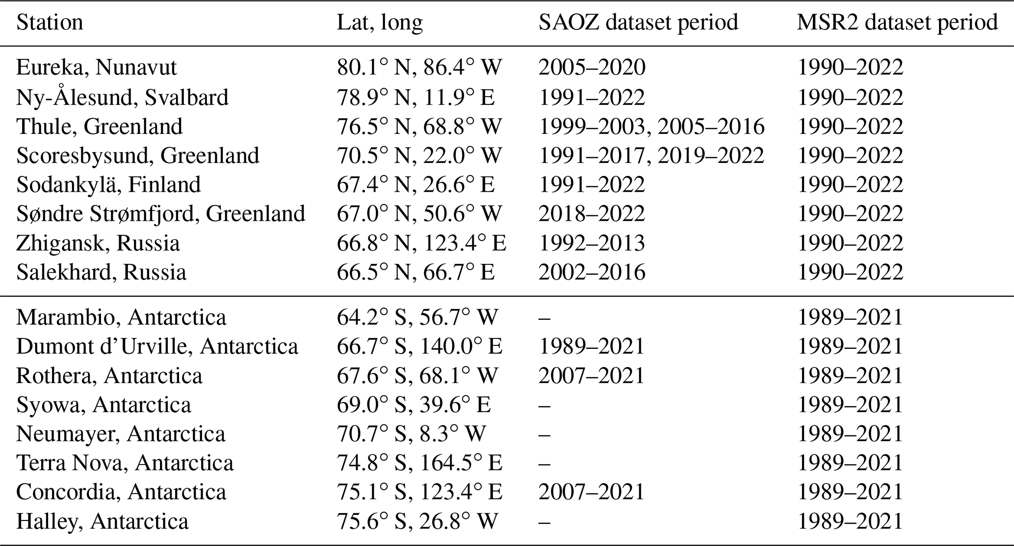
The difference between sunset and sunrise NO₂ total columns is calculated at each SAOZ station to follow the amplitude of the NO₂ diurnal cycle and to assess whether denitrification, which could promote ozone loss, occurred inside the vortex. SAOZ data are available on the NDACC database (https://www-air.larc.nasa.gov/missions/ndacc/, last access: 24 February 2023) and the SAOZ web page (http://saoz.obs.uvsq.fr/, last access: 24 February 2023).

2.2 Multi-Sensor Reanalysis (MSR2)

In this study, daily SAOZ total column ozone data corresponding to the mean sunrise–sunset values are merged with daily MSR2 ozone columns. The MSR2 ozone dataset comprises daily assimilated gridded ozone columns at 12:00 UT at a spatial resolution of 0.5^∘ × 0.5^∘ in both hemispheres. The TM3-DAM CTM (simplified version of TM5; Krol et al., 2005) is used to assimilate 14 polar-orbiting satellite datasets, already corrected for SZA dependency, stratospheric temperature, and other parameters by means of comparisons with ground-based datasets from Dobson and Brewer networks, which are part of the World Ozone and Ultraviolet Data Center (WOUDC) (see van der A et al., 2010, 2015, for a detailed description). The data covering the 1989–2022 period are available from the Tropospheric Emission Monitoring Internet Service (TEMIS) of KNMI/ESA (http://www.temis.nl, last access: 4 March 2023).

Daily ozone columns at the stations mentioned in Table 1 are retrieved from the global gridded MSR2 assimilated data fields by averaging the total ozone columns of MSR2 within ±1^∘ of the station coordinate. Data corresponding to the grid cell with forecast error estimates higher than 20 DU for MSR2 were removed following indications given on the TEMIS/ESA website. This filter was increased to 35 DU for 1993–1994 in the Southern Hemisphere (SH) to allow for data in July for purposes of normalisation (see Sect. 3, Methodology).

2.3 TOMCAT/SLIMCAT model

The three-dimensional offline CTM TOMCAT/SLIMCAT (Chipperfield, 1999) (hereafter SLIMCAT) is used to simulate passive odd-oxygen tracer that is transported and/or advected without any interactive chemistry (Feng et al., 2005) and active ozone with full stratospheric chemistry, including heterogeneous reactions on sulfate aerosols and polar stratospheric clouds (PSCs) (Feng et al., 2021). In this study, SLIMCAT is forced by wind and temperature fields from the European Centre for Medium-Range Weather Forecasts (ECMWF) ERA5 reanalysis (Hersbach et al., 2020). The model uses a hybrid σ-pressure as the vertical coordinate. The tracer advection uses the scheme of the conservation of second-order moments by Prather (1986). The vertical transport is diagnosed using mass flux divergence (Chipperfield, 2006).

The long-term simulations used in this work start in 1980 (Feng et al., 2021) with a horizontal resolution of 2.8^∘ latitude × 2.8^∘ longitude and 32 vertical levels from the surface to ∼ 65 km. The passive ozone tracer is preinitialised each year on 1 July in the Southern Hemisphere (SH) and on 1 December in the Northern Hemisphere (NH) by setting it to be equal to the modelled active chemical ozone field. The passive and active ozone columns are sampled above the stations of Table 1 at 12:00 UT by performing a bilinear interpolation of the model fields (in latitude and longitude) to the location of the SAOZ stations during the model simulation. The SLIMCAT model has been widely used in previous studies of stratospheric ozone (e.g. Feng et al., 2021).

3 Methodology

The ozone loss is obtained by applying the passive-tracer method (Goutail et al., 1999), which has been applied in different studies to calculate ozone loss in the SH (e.g. Kuttippurath et al., 2010, 2013) and the NH (e.g. Pommereau et al., 2013, 2018) using MSR2 or SAOZ data. The loss is computed at each station of Table 1 by subtracting the measured total ozone (SAOZ and MSR2 merged dataset, hereafter called OBS) inside the polar vortex from the corresponding passive ozone column simulated by SLIMCAT. To determine if the station is inside the vortex, the Nash et al. (1996) criterion is applied on the equivalent-latitude (EL)–isentropic-level (θ) quasi-conservative coordinate system (McIntyre and Palmer, 1984). This system can be assimilated to 2-D vortex-following coordinates where the pole corresponds to the position of maximum potential vorticity (PV). The wind and temperature fields from ERA5 reanalysis are used to calculate the 2-D coordinate system. The vortex edge is considered to be the limit between a region inside and outside the vortex, corresponding to the EL of the maximum PV gradient, weighted by the wind module temporally smoothed with a 5 d moving average, as described in Pazmiño et al. (2018). Similarly to previous works (e.g. Kuttippurath et al., 2010; Pommereau et al., 2013), the classification of the station with respect to the position of the vortex is considered at the 475 K isentropic level (∼ 18 km), where the ozone maximum is observed in winter–spring. Figure 1 shows the number of merged data inside the vortex for each winter of the considered periods for the SH (blue line) and NH (red line). Between 200 and 400 observations are considered for the Arctic vortex, and about 800 are considered for the Antarctic vortex. The number of observations in the Arctic vortex displays a large interannual variability, while it is much more stable in the Antarctic. These differences are explained by the larger area and the longer persistence of the SH vortex compared to the NH one.

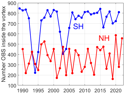
Figure 1 Number of merged data (OBS) inside the vortex for each winter of the SH (blue line) and NH (red line).

Before the subtraction, the SLIMCAT passive ozone tracer is normalised to the MSR2 ozone dataset. The normalisation coefficient is calculated at each station considering the difference between the monthly mean values of the MSR2 ozone and SLIMCAT active ozone tracer in December (July) for the NH (SH). SAOZ measurements are also normalised by the mean difference between MSR2 and SAOZ data at the beginning of each winter (December/July for NH/SH) or, if not available at high latitudes, in March (August) in the NH (SH). In the case of the days when only one measurement is available, the corresponding value is considered. The amplitude of the mean monthly difference during the winter between normalised SAOZ data and MSR2 or merged data is less than 2 % or 1 %, respectively, which is smaller than the SAOZ precision (Hendrick et al., 2011).

Figure 2 shows the evolution of MSR2 and SAOZ ozone observations and normalised ozone columns (both passive and active) from the model at Ny-Ålesund during the Arctic winter of 2021–2022. Panel a shows the position of the station and the vortex edge on the equivalent latitude scale at the 475 K isentropic level. The SLIMCAT tracer captures the short-term ozone fluctuations resulting from horizontal and vertical transports linked to the propagation of the planetary waves. The horizontal transitions between regions inside and outside the vortex are observed by mid-March (day ∼ 70), with ozone values increasing from ∼ 300 to ∼ 550 DU. The progression of chemical ozone loss (100 × (passive tracer − OBS) $/$ passive tracer) above the station is observed to reach 112 DU on Julian day 83, corresponding to about 23 % (Fig. 2c). The agreement observed between the MSR2 and SAOZ datasets after normalisation gives confidence in this simple method in terms of building the OBS merged dataset. The mean biases between MSR2 and the normalised SAOZ datasets in the NH are within ±0.3 DU at each station, and in the SH, they are between 0 and −1 DU, with a standard deviation of the mean lower than 1 DU.

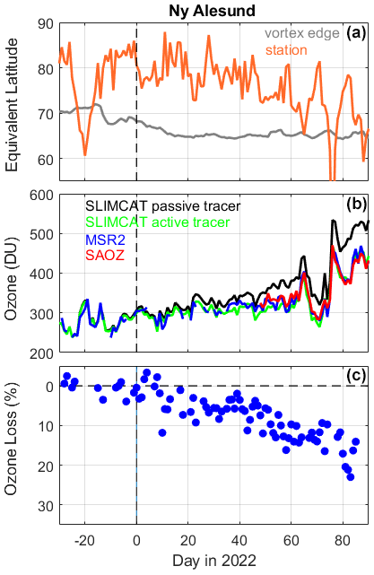
Figure 2 (a) Evolution of the position of the 2021–2022 vortex edge over Ny-Ålesund station in equivalent-latitude scale at the 475 K isentropic level. (b) Evolution of ozone columns at Ny-Ålesund from reanalysis MSR2 fields, SAOZ observations, and simulations by SLIMCAT in 2021–2022. (c) Evolution of ozone loss (in %) at Ny-Ålesund derived from OBS merged dataset (see the text) and the SLIMCAT passive tracer in 2021–2022 winter.

The relative ozone losses at each station (Table 1) within the vortex are considered altogether, and a 10 d running median is applied during the winter. Figure 3 shows the evolution of the relative ozone loss during the 2022 NH winter (black line) obtained from the ozone loss values above the different stations (symbols in colour). At the end of the winter, the accumulated ozone loss is considered to be complete when temperatures within the vortex are higher than the temperature threshold for nitric acid trihydrate (NAT) PSC formation (T_NAT). At that time, the diurnal NO₂ difference rapidly increases (Fig. 3b), and ClO values from SLIMCAT rapidly decrease (not shown). During the 2022 NH winter, a fast increase of the diurnal NO₂ difference is observed after day 60 (as shown in Fig. 3b) as a signature of chlorine deactivation. Long periods were also observed in which minimum temperatures were lower than T_NAT inside the vortex for 105 and 81 d at the 475 and 550 K isentropic levels, respectively, as shown in Fig. 4a. The considered thresholds are 195 and 192 K for the 475 and 550 K isentropic levels, respectively (Pommereau et al., 2013). PSC formation stops first at the higher levels on day 50 and then later on day 75 at the lower levels. The accumulated ozone loss observed on day 80 reaches 18.1 ± 0.5 % (87 ± 2.7 DU). The standard error of the median corresponding here to half of the Q₈₄–Q₁₆ ​​​​​​ or 68 % interpercentile spread (IP68) is also shown.

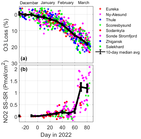
Figure 3 (a) Time series of observed ozone loss (%) inside the vortex above each SAOZ station for the 2022 NH winter. (b) Time series of the amplitude of the NO₂ diurnal variation (NO₂ sunset – NO₂ sunrise) inside the vortex above SAOZ stations. The 10 d running median and standard error of the median (IP68/2; see the text) are superimposed by the black line on both panels.

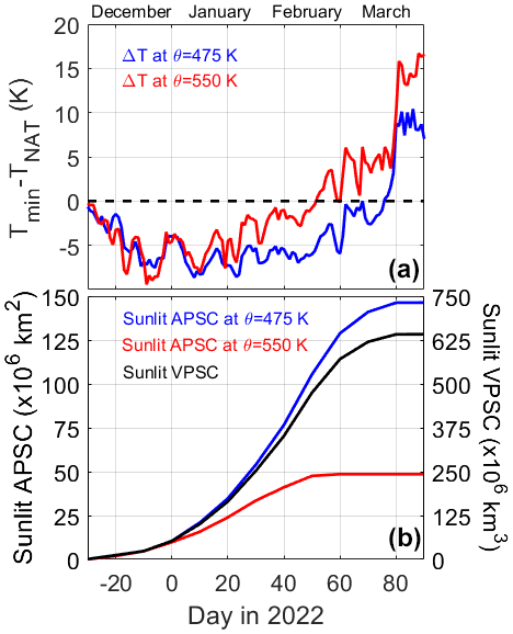
Figure 4 (a) Time series of difference between minimum temperatures and T_NAT (K) at 475 and 550 K isentropic levels for the 2022 NH winter. Negative values correspond to the period of PSC formation at the corresponding isentropic level. (b) Cumulative time series of sunlit areas of PSC at 475 (blue) and 550 K (red). The sunlit volume of VPSC computed following Rex et al. (2004) is superimposed by a black curve.

The interannual behaviour of ozone loss related to PSCs, which plays a crucial role in ozone polar heterogeneous chemistry, is also analysed. The cumulative surface of the polar vortex exposed to temperatures lower than the NAT PSC formation threshold coincident with sunlit regions (SZA < 93^∘) was computed at 475 and 550 K. This cumulative surface is hereafter referred to as sunlit APSC_θ. The APSCs on the 475 and 550 K isentropic levels are shown in Fig. 4b for the 2022 NH winter. The sunlit NAT PSC volume (sunlit VPSC) was estimated following the relationship of Rex et al. (2004) and integrated through the end of the winter. The sunlit VPSC is considered to be a proxy of chlorine activation. The computed VPSC for the 2022 NH winter is superimposed on Fig. 4b (black curve).

4 Polar ozone loss in the 2018–2022 period

Since 2000, an increasing interannual ozone loss variability has been observed in both hemispheres, particularly in the SH, compared to previous winters. Figure 5 presents the evolution of ozone loss calculated by our method between 2018–2021 in the SH (panel a) and 2018–2022 in the NH (panel b). Ozone losses in previous atypical years are also shown (dotted lines), e.g. the NH 2011 record ozone loss (Pommereau et al., 2013) that was due to a cold, strong, and long-lasting polar vortex (Manney et al., 2011) and the 2002 SH weak ozone loss (Hoppel et al., 2003) that was linked to unprecedented large-wave activity (Allen et al., 2003) which resulted in a major sudden stratospheric warming (SSW) and a split of the vortex in the middle stratosphere at the end of September. The median values of ozone loss for the 1989–2017 winters in the SH and the 1990–2017 winters in the NH and the corresponding 20th and 80th percentiles are also represented in Fig. 5 by the black lines and shaded area, respectively. Similarly to Fig. 5, the $T_{min}-T_{\mathrm{NAT}}$ anomaly at 475 K is shown for the last winters in Fig. 6, and the 45 d mean heat flux in the 45–75^∘ latitude range at 70 hPa from MERRA-2 analyses (NASA's Goddard Space Flight Center, https://acd-ext.gsfc.nasa.gov/Data_services/met/ann_data.html, last access: 6 October 2022) is shown in Fig. 7 to evaluate the impact of dynamical activity. Figure 8 plots the proxy GRAD (gradient) corresponding to the maximum gradient of PV as a function of equivalent latitude within the vortex boundary region (Pazmiño et al., 2018) to evaluate the stability of the vortex during the study period. Pazmiño et al. (2018) used both proxies to characterise the interannual evolution of total ozone in Antarctica during the September and October periods.

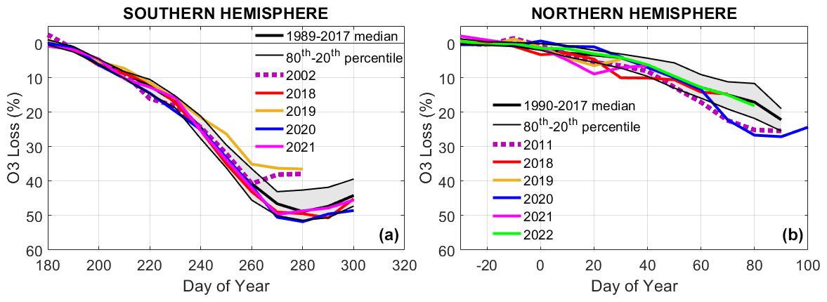
Figure 5 Evolution of ozone loss in recent winters using the merged OBS dataset: SH 2018–2021 (a) and NH 2018–2019 and 2021–2022 (b). Unusual winters are also represented by dashed pink lines: weak ozone loss in SH (2002) and 2011 record ozone loss in NH. The median and 20th–80th percentile climatological values of previous winters are represented by thick and thin black lines, respectively.

Figure 6 As Fig. 5 but for temperature anomaly at 475 K using ERA5 reanalyses.

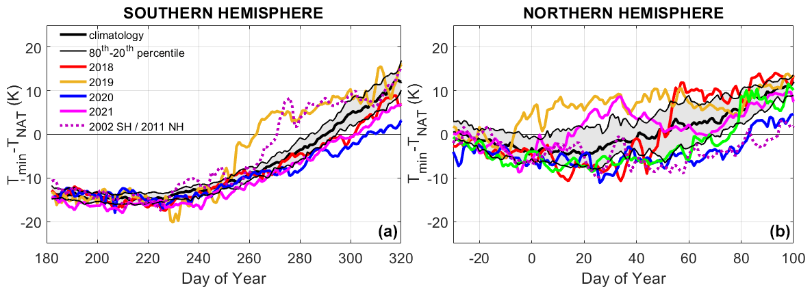
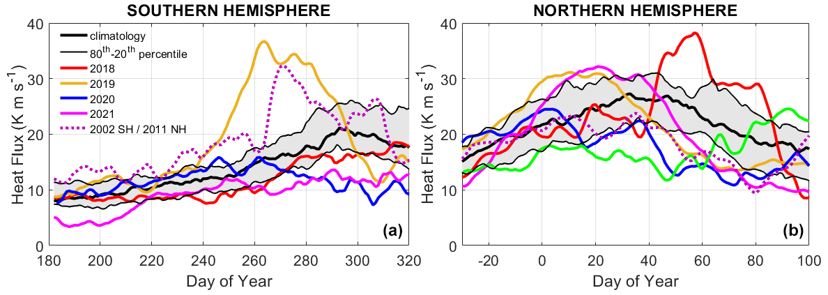
Figure 7 As Fig. 5 but for 45 d mean heat flux in the 45–75^∘ latitude range at 70 hPa from MERRA-2 analyses.

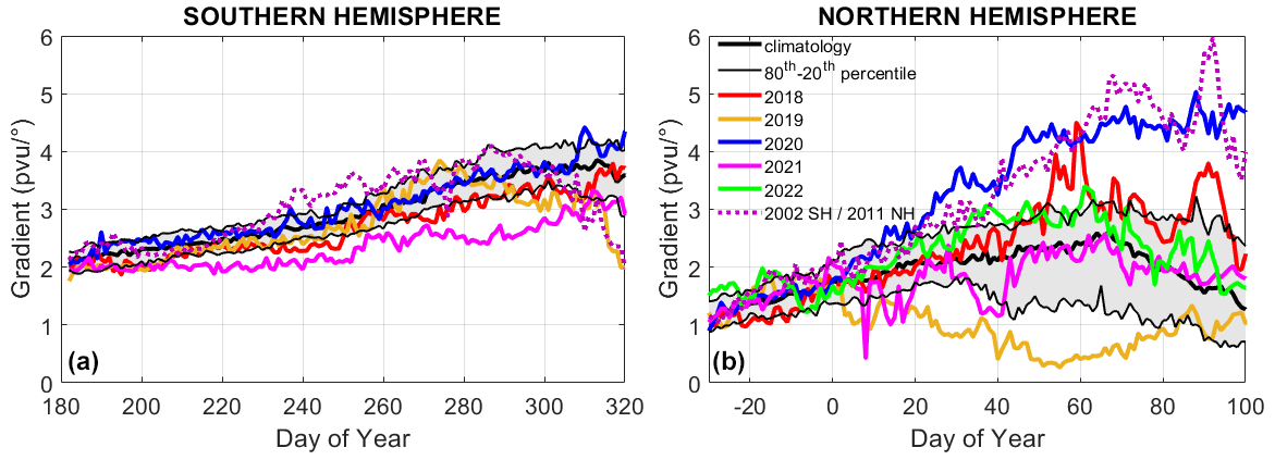
Figure 8 As Fig. 5 but for the PV gradient in the vortex edge as defined in Pazmiño et al. (2018) using ERA5 reanalyses.

The median value of the accumulated ozone loss at the end of the winter is more than 2 times larger in the SH than in the NH. The recent winters present an accumulated ozone loss varying from 7 % to 27 % in the NH and 37 % to 52 % in the SH. The maximum ozone loss is reached between mid-January and the end of March for the NH and between the end of September and mid-October for the SH. The interannual variability of the ozone loss represented by the maximum amplitude of ozone loss between the recent winters is mostly similar in both hemispheres: 20 % in the NH and 15 % in the SH.

4.1 Southern Hemisphere

In the SH (Fig. 5a), the evolution of the ozone loss during the recent winters is found to be within the climatological values (grey area) until the end of August (day 240). For the 4 years shown, temperatures lower than T_NAT are observed early, from mid-May, at the 475 K isentropic level.

The 2018 SH winter is a typical one (cold winter with a strong vortex) close to the median climatological value, reaching a maximum ozone loss of 50.7 ± 1.1 (1σ) % at day 290 (red line). Temperature values lower than T_NAT persist until the end of October, as shown by $T_{min}-T_{\mathrm{NAT}}$ anomalies at 475 K in Fig. 6a. The anomaly is within the 20th–80th percentiles of the 1989–2017 climatological median values represented by the grey area. The mean anomaly was −10.1 ± 4.8 K for 174 consecutive days. The dynamical activity was near the climatology (Fig. 7a) and so was the vortex stability (Fig. 8a).

During the 2019 SH winter, a minor SSW appeared at the end of August, linked to wavenumber-1 event, producing a displacement of the vortex at the upper levels with an associated decrease in size. These two factors were similar to the 2002 SH winter (dashed pink line in Fig. 5a), where a major SSW occurred at the end of September, inducing large total ozone values within the vortex (Wargan et al., 2020). In 2019, after the minor SSW at the end of August, the ozone loss started to slow down, as shown by a levelling of the ozone loss, diverging from the climatological grey area and reaching a maximum of 36.3 ± 1.3 % in the first week of October (brown line in Fig. 5). In the case of 2002, the ozone loss stopped rapidly after the major warming and reached a slightly larger ozone loss compared to 2019. The period with temperatures lower than T_NAT was reduced by 1 month compared to 2018 and displayed a mean T anomaly slightly higher than in 2018 (−11.4 ± 4.2 K over 132 consecutive days). The dynamical activity is well represented in Fig. 7, where the heat flux increases rapidly at the end of August with values that are much higher than the climatology until mid-October and that are comparable to the NH (Fig. 7b). The stability of the vortex was within the climatological values until mid-October, slowing down rapidly thereafter.

The SH stratosphere in 2020 was strongly impacted by the enhancement of aerosol levels from the severe southeastern Australia bushfires during 29 December 2019 to 4 January 2020, known as the Australian New Year (ANY) fires (e.g. Khaykin et al., 2020). Rieger et al. (2021) showed ozone negative anomalies in mid-latitudes and polar regions from OMPS satellite observations linked to the ANY event; these were of magnitudes similar to the anomalies related to the Calbuco volcanic eruption in April 2015 in the south of Chile. In the Antarctic, the 2020 winter ozone loss evolution was within climatological values until the end of September (blue line in Fig. 5). Temperatures lower than T_NAT were already present in May until the beginning of November (176 d), with a mean T anomaly of −10.1 ± 4.5 K, as in 2018 but with a much larger sunlit VPSC than in 2018. The maximum ozone loss of 51.8 ± 1.4 % was found in early October, a value outside the 20th–80th percentile range of the climatology. The persistently cold lower stratosphere in the polar region in 2020 led to an acceleration of the October ozone loss and a delayed break-up of the polar vortex, explaining the long-lasting ozone loss during the months of October to November (Damany-Pearce et al., 2022). The heat flux exhibited values within the climatology until the end of September before slowing down rapidly during October (Fig. 7), and the strength of the vortex edge was close to the median climatological value (Fig. 8).

During the 2021 SH winter, the evolution of ozone loss was within the climatological values until the end of August (day 240). The temperatures lower than T_NAT started later than previous years in May, persisting until the end of October, as in 2018 and 2020, with a T anomaly of −11 ± 5.3 K corresponding to 167 d (Fig. 6). The ozone loss ratio increased between the end of August and the beginning of October (day 270), reaching the lower limit of climatological ozone loss values. The sunlit VPSC values were similar to those of 2018, but the strength of the vortex was weaker than in previous years, as shown by the low PV gradient in Fig. 8. This year also presented lower heat flux values than the climatology before August and after mid-September (Fig. 7), and the final accumulated ozone loss reached 49.7 ± 0.9 % (pink line in Fig. 5), which lies within the climatology.

4.2 Northern Hemisphere

In the NH (Fig. 5b), the evolution of the accumulated ozone loss is strongly dependent on the temperature history. The ozone loss already starts to vary from one year to the next in December. Perturbed winters due to enhanced wave activity could favour mixing across the polar vortex.

The 2018 NH winter (red line in Fig. 5b) displayed higher ozone loss than the 20th–80th interpercentiles (grey area) from mid-December to mid-February. Temperatures within the vortex at the 475 K isentropic level were much lower than the T_NAT threshold from early December until mid-February, with a mean T_min anomaly of −5.3 K (Fig. 6b). The major SSW on 12 February, linked mainly to wavenumber-2 forcing (Butler et al., 2020), induced a rapid increase in temperature and a split of the vortex. This increase in dynamical activity is also highlighted by the increase in the heat flux (Fig. 7). The strength of the vortex exhibited values larger than climatology (Fig. 8). The very low temperatures for the remaining ∼ 80 d within the vortex allowed moderate ozone loss of 14.7 ± 0.8 (1σ) %.

The 2019 NH winter also presented an SSW but early in the year corresponding to the January single warming mode (Mariaccia et al., 2022), as shown by the increase in heat flux outside the climatological values at the end of December (brown line in Fig. 7). The major SSW of 2 January 2019 was linked to a wavenumber-1 event (Butler et al., 2020). The vortex weakened more rapidly after the SSW and remained at low values thereafter (Fig. 8). Temperatures lower than T_NAT were observed during 20 (non-consecutive) days in December, with a mean anomaly value of −2.2 K at the 475 K isentropic level (Fig. 6). The accumulated ozone loss of the 2019 warm winter was 6.5 ± 1.4 % (Fig. 5).

The 2020 NH winter is associated with record-low ozone values within the vortex, which are explained by a long period of temperatures lower than T_NAT from December to mid-March (113 d at 475 K isentropic level, blue line in Fig. 6), a large stability of the vortex (Fig. 8), and a low ozone resupply from lower latitudes (e.g. Manney et al., 2020). In the beginning of December, temperature anomalies at the 475 K level were near −4 K, and the mean anomaly value for the whole winter reached −5.3 K, as in 2018. The ozone loss was within the climatological values until March, but a rapid increase of 13 % during March led to an accumulated ozone loss of 27.1 ± 1.1 % (Fig. 5). Mariaccia et al. (2022) classified this winter as an unperturbed radiative final warming mode, also shown by the low values of the heat flux in Fig. 7. Comparing the 2020 and 2011 winters with pronounced ozone loss (dashed pink line in Fig. 5), we find a similar maximum ozone loss at the end of March, which is due to the persistent low temperatures less than T_NAT for ∼ 110 d (Fig. 6), a weak dynamical activity (Fig. 7), and a strong vortex (Fig. 8).

The 2021 NH winter experienced a major SSW on 5 January (pink line in Fig. 6). Temperatures lower than T_NAT were observed during 41 consecutive days between early December and mid-January, with a mean value of T anomaly of −3.4 K (Fig. 7). During this period, a rapid ozone loss evolution outside the climatological values was observed at the beginning of January, slowed down by the SSW event that stopped it on 20 January (Fig. 5). The accumulated ozone loss was only 8.9 ± 1.2 %.

The 2022 NH winter is associated with an unperturbed dynamical final warming mode, as shown by the low values of heat flux until the beginning of March (day 60) (green line in Fig. 7). It was a cold and long-lasting winter, with temperatures lower than T_NAT until mid-March (105 d at 475 K, Fig. 6), with a mean value of −6.5 K for the T anomaly. The ozone loss is well within the climatological values, with an accumulated ozone loss of 18.1 ± 0.5 % (Fig. 5).

5 Long-term evolution of ozone loss

In order to study a possible recovery rate of total ozone columns in the polar regions, three different metrics were applied to the ozone loss datasets. Then, a robust linear fit was calculated from 2000, the year of maximum ODS amounts in the polar stratosphere (WMO, 2014).

5.1 Maximum ozone loss

The first metric considered is the maximum ozone loss (MOLoss) for each winter, which corresponds to the maximum value of the accumulated ozone loss within the respective winter period, as considered in Sect. 3. Figure 9 shows the interannual evolution of MOLoss for both hemispheres (coloured lines). The model results using its active tracer are also represented (grey lines). A good agreement is observed in the interannual variability of observations and simulations in both hemispheres, with systematically smaller values in the simulations since 2003 in the SH. As expected, the NH MOLoss shows smaller values but larger interannual variability, which is intrinsically linked to a more disturbed stratospheric dynamic.

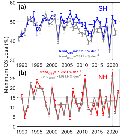
Figure 9 Interannual evolution of the maximum ozone loss obtained using the passive-tracer method and the merged OBS dataset (colour lines) and model (grey line) in the SH (a) and NH (b). The estimated robust trends since 2000 were added to the figures with the corresponding colour codes.

In the SH, a stabilisation of the MOLoss is observed in the 1990s at about 50 %, and a slight decrease can be seen from 2000, with an enhanced interannual variability in the last decade. A similar negative trend in ozone loss is found based on observed (OBS) and modelled results, with values of −2.3 ± 1.5 % and −2.8 ± 1.4 % per decade, respectively. The trends are significant only at 1 standard deviation (σ) for the OBS. In particular, the SSW years 2002 and 2019 are characterised by smaller MOLoss values, followed by 2004, 2012, 2013, and 2017. The years 2002, 2004, 2012, and 2013 were identified by Lim et al. (2019) as years that had a weak SH polar vortex. In 2017, the heat flux (not shown) presents values higher than the climatological envelope from the end of August to the end of September, with T anomalies rapidly increasing by 8 K with respect to the median in the second half of September, which could have slowed down the chemical ozone depletion.

In the NH, the average MOLoss is less than half of that observed in the SH. The large ozone losses in the mid-1990s NH are shown in Fig. 9b, with values near 20 %. There is substantial interannual variability between warm and cold winters, with two record values of ozone loss in 2011 and 2020. The trend values estimated since 2000 are positive (1.2 ± 2.1 % per decade), but they are not significant. This metric does not allow the detection of any trend in the NH.

5.2 Ozone loss onset day

The ozone loss onset day (OLossOnset) metric was developed to analyse the evolution of the ozone loss at different thresholds values as we might expect a later onset of polar ozone loss in relation to lower amounts of ODS in the stratosphere. The onset day is determined to be the day when the 10 d running median ozone loss crosses a determined threshold value. A similar metric for total ozone values inside the vortex was used in a previous study (Pazmiño et al., 2018). In this study, the dataset of ozone loss onset days is used instead of the dataset of total ozone column onset days in order to consider chemical processes only. Figure 10 presents the evolution of OLossOnset at five different thresholds of ozone loss for the SH (panel a) and NH (panel b).

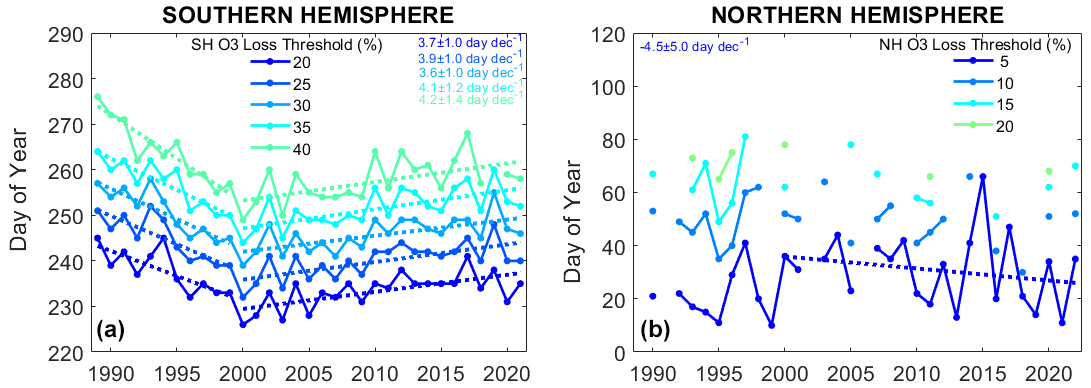
Figure 10 Onset day when 10 d averaged ozone loss reaches a particular ozone loss value: 20 %, 25 %, 30 %, 35 %, and 40 % for the SH (a) and 5 %, 10 %, 15 %, and 20 % for the NH (b). Robust linear fits before and after 2000 are also shown for the SH (dashed lines).

In the case of the SH, the chosen ozone loss threshold values enable a long-term estimation of the interannual evolution of OLossOnset. The trend estimations were performed before and after 2000. All trends estimated by independently robust linear regression are significant at at least 2σ. The lower trend values are observed for the threshold of 20 % and the highest ones for the threshold of 40 % of ozone loss before and after 2000. The positive trends vary between 3.6 ± 1.0 and 4.2 ± 1.4 d per decade. The ratio between the trends before and after 2000 for each OLossOnset dataset is −0.3, with the exception of the threshold of 40 %, where −0.2 is found due to the steeper slope observed before 2000. The onset dataset obtained from SLIMCAT model simulations exhibits larger trends since 2000 that are significant at 2σ (not shown). The trends vary from 4.4 ± 1.0 to 6.1 ± 1.8 d per decade. The ratios between the trends before and after 2000 for each ozone loss onset dataset vary from −0.5 to −0.3, showing a faster recovery considering SLIMCAT simulations compared to using the SAOZ-MSR2 merged dataset, as already found using the ozone loss metric 1 (see Sect. 5.1). For the NH, only the OLossOnset at the threshold of 5 % is reached almost every year of the considered period. The trend observed is marginally significant (−4.5 ± 5.0 d per decade). The other thresholds do not allow any robust statistical analysis. This metric does not allow the detection of any trend in the NH.

5.3 Residuals of ozone-loss–VPSC relationship

Climate change can influence the polar ozone loss through changes in temperature within the vortex, which directly influence the formation of PSCs. Figure 11 represents the interannual evolution of sunlit VPSCs above the Antarctic and Arctic regions (panels a and b, respectively). Larger sunlit VPSC values are expected in the SH than in the NH due to much lower polar temperatures. Low values of sunlit VPSCs are found for the years of low ozone loss, and the inverse is also true, as expected (see Fig. 9). Record values of sunlit VPSCs are observed in 2020 for both hemispheres. As a consequence, very high ozone loss was found in the NH, and large but not record ozone loss was found in the SH. A linear trend was computed for VPSCs from 2000, yielding an insignificant value in the SH and a positive value in the NH, though these were significant only at the 1σ level.

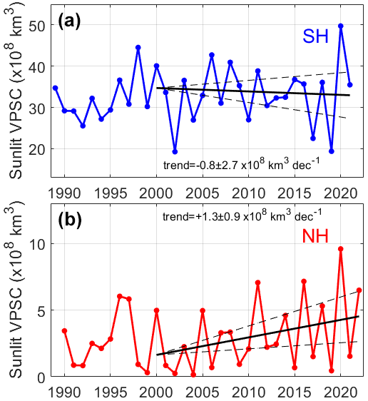
Figure 11 Interannual evolution of sunlit volume of polar stratospheric clouds (VPSCs) in the SH (a) and NH (b). The estimated robust trend (thick black line) and uncertainty level values of ±1σ (dashed black lines) since 2000 are added for both regions.

Figure 12 presents the ozone loss value as a function of sunlit VPSCs for each winter of the NH (triangles) and SH (inverse triangles). The figure highlights the difference between both hemispheres, with many more sunlit VPSCs in the SH and, consequently, more ozone loss. The range of sunlit VPSCs in the SH varies between 2 × 10⁹ and 5 × 10⁹ km³, which corresponds to an ozone loss between 36 % and 55 %. The range of sunlit VPSCs in the NH is much smaller (< 10⁹ km³), but the dynamical range of ozone loss is slightly higher (4 %–27 %). The figure highlights a quasi-linear relationship between ozone loss and VPSCs in the NH (lower-left region in Fig. 12) and a different behaviour for larger ozone loss values due to the saturation of ozone loss in the lower stratosphere in the SH (e.g. Yang et al., 2008).

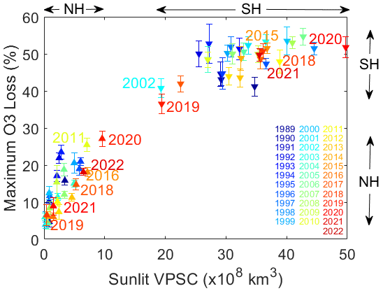
Figure 12 Maximum ozone loss as a function of sunlit VPSCs for each winter for the Northern and Southern hemispheres. The 68 % interpercentile range of ozone losses is also represented (see Sect. 3, Methodology). The colour code represents the years.

In order to remove the influence of temperature interannual variability in the estimation of trends since 2000, a multi-parameter model was applied to the ozone loss dataset of each region, as presented in Eq. (1):

$$\begin{array}{}\text{(1)}& \begin{array}{rl}\mathrm{MOLoss}\left(t\right)& =\mathrm{SunlitVPSC}\mathrm{\_}\mathrm{contr}\left(t\right)\\ & +t\mathrm{1}\times \left(\mathrm{year}\right(t)-\mathrm{2000})+\in \left(t\right),\end{array}\end{array}$$

where t is the number of years since 2000, t1 is the time-linear trend since 2000, ∈(t) is the ozone loss residual, and SunlitVPSC_contr corresponds to the contribution of sunlit VPSCs considering a linear fit for the NH and a parabolic fit for the SH due to the saturation of ozone loss in the lower stratosphere (Eqs. 2 and 3, respectively).

$$\begin{array}{}\text{(2)}& {\displaystyle }\begin{array}{rl}\mathrm{SunlitVPSC}\mathrm{\_}\mathrm{contrNH}\left(t\right)& =K_{\mathrm{0}\mathit{\_}\mathrm{NH}}\\ & +K_{\mathrm{1}\mathit{\_}\mathrm{NH}}\times \mathrm{SunlitVPSC}\mathrm{\_}\mathrm{NH}\left(t\right)\end{array}\text{(3)}& {\displaystyle }\begin{array}{rl}\mathrm{SunlitVPSC}\mathrm{\_}\mathrm{contrSH}\left(t\right)& =K_{\mathrm{0}\mathit{\_}\mathrm{SH}}\\ & +K_{\mathrm{1}\mathit{\_}\mathrm{SH}}\times \mathrm{SunlitVPSC}\mathrm{\_}\mathrm{SH}\left(t\right)\\ & +K_{\mathrm{2}\mathit{\_}\mathrm{SH}}\times \mathrm{SunlitVPSC}\mathrm{\_}\mathrm{SH}(t{)}^{\mathrm{2}}\end{array}\end{array}$$

The regression coefficients in Eqs. (2) and (3) are significant at the 2σ level. The autocorrelation of residuals of ozone loss in Eq. (1) is weak and lower than 0.2, and the determination coefficient (R²) is 0.83 for the SH and 0.82 for the NH. Figure 13a and c show a good agreement between the MOloss dataset (colour lines) and the regression model results (black lines) considering estimated sunlit VPSC contribution (dashed black line) and trend.

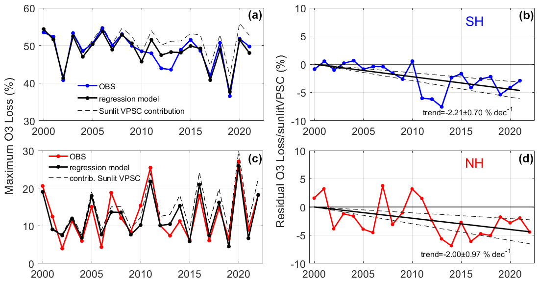
Figure 13 (a, c) Interannual evolution of the maximum ozone loss (colour lines) since 2000 for both hemispheres and the regression model (black lines). Sunlit VPSC contribution (see Eq. 2 for NH and Eq. 3 for SH) is superimposed by dashed lines. (b, d) Interannual evolution of residuals of ozone loss with respect to regressed ozone loss values computed following Eqs. (1) to (4) for the SH (a, b) and the NH (c, d). The estimated trend (thick black line) and uncertainty level values of ±1σ (dashed black lines) since 2000 are also represented for both hemispheres.

The difference between the maximum ozone loss and the regressed sunlit VPSC contribution (ROLoss) is calculated for each year of the corresponding hemisphere as follows:

$$\begin{array}{}\text{(4)}& \begin{array}{rl}\mathrm{ROLoss}\left(t\right)& =\mathrm{MOLoss}\left(t\right)-\mathrm{SunlitVPSC}\mathrm{\_}\mathrm{contr}\left(t\right)\\ & =t\mathrm{1}\times \left(\mathrm{year}\right(t)-\mathrm{2000})+\in \left(t\right).\end{array}\end{array}$$

Figure 13b and d show the ROLoss dataset for the SH (panels a and b) and the NH (panels c and d), respectively. The residuals vary between approximately 0 % and −8 % for the SH and within ±5 % for the NH. A decrease is observed since 2000 in both hemispheres, with a higher interannual variability in the NH. The linear trend estimated by the multi-parameter regression model in both hemispheres (Eq. 1) is around 2 % per decade and is significant at 2σ. Unlike the other two metrics, this metric provides a potential detection of a negative trend in the NH at the limit of significance.

The multi-parameter model was also applied to ozone loss using only SLIMCAT simulations (not shown). All regression coefficients are significant at 2σ, except the quadratic regression coefficient in the case of the SH. A larger recovery rate is found with the model simulation in the SH, with a negative trend of −2.8 ± 0.8 % per decade (1σ). For the NH, a slightly weaker trend was found compared to the observations, with a value of −1.4 ± 0.7 % per decade, also with limited significance at 2σ.

6 Conclusions

Ozone loss datasets extending for more than 30 years were computed for both polar regions using the passive-ozone-tracer values simulated by the SLIMCAT CTM combined with SAOZ ground-based data merged with the MSR-2 reanalysis. Although the passive-tracer method enables the identification of ozone evolution due only to chemistry, this chemistry can be influenced by dynamical processes via their effect on temperature. The ozone loss shows a linear relationship with sunlit VPSCs within the vortex for the NH and a parabolic behaviour in the SH due to the saturation effect of the ozone loss in the Antarctic stratosphere.

The analysis of ozone loss in the polar winters since 2018 shows that much of the loss lies between the 20th and 80th percentiles of the values observed in previous years and that they are well correlated with the temperature history (Figs. 5 and 6). The extreme years are prominent in the ozone loss datasets with (1) an atypical weak ozone loss in the 2019 SH caused by an early minor SSW at the end of August due to the strong dynamical activity in that year, comparable to what is generally observed in the NH (Fig. 7), and (2) a large ozone loss in 2020 in both hemispheres with 7 % higher values than the median climatology, linked to very cold and long-lasting winters. Notably, the strength of the vortex edge in the 2020 NH is larger than the values observed in the SH climatology, including those of the year 2020 (Fig. 8).

In order to estimate a possible recovery of ozone, trends since 2000 were computed for three different metrics. In the first case, based on the maximum ozone loss found at the end of the winter, a negative trend of −2.3 ± 1.5 % per decade was found in the SH, only significant at 1σ. This metric appears to be sensitive to dynamics since the maximum in ozone loss generally occurs between days 270–290, in October, a month characterised by higher temperatures within the vortex and larger transport variability (Solomon et al., 2016). Regarding the NH, a positive trend of +1.2 ± 2.1 % per decade was calculated, but it is not significant. This positive trend is mostly influenced by the record ozone loss years of 2011 and 2020. The second metric takes into account the interannual evolution of the onset day when the ozone loss reaches different thresholds, similarly to the methodology developed for total ozone values by Pazmiño et al. (2018). In the SH, this metric shows a positive trend of +3.8 ± 1.0 d per decade on average. This trend is significant at 2σ and could be related to the lower ODS amounts in the polar austral stratosphere compared to the period before 2000. The various thresholds are reached in September so this metric is sensitive to the ozone loss at a time that is less affected by dynamical processes compared to October, when the maximum ozone loss is reached. In the NH, this metric does not show a statistically significant trend due to the large interannual variability and the fact that most of the thresholds are not reached in the period studied. The third metric takes into account the relationship between ozone loss and the sunlit volume of PSCs, linked to heterogeneous chemical processes. In the SH, the ozone loss residuals show a negative trend from 2000 of −2.2 ± 0.7 % per decade, significant at 2σ, indicating a statistically significant signal for the recovery of ozone. This value is close to that obtained with the first metric. In the case of the NH, for the first time, a potential recovery is observed based on this metric, which displays a trend of −2.0 % per decade; this is slightly significant at 2σ. Note that this trend is similar to the SH trend.

In conclusion, our study confirms the ozone recovery in the SH, which is significant for two of the three metrics based on the ozone loss datasets despite the higher interannual variability in the last decade. In the NH, our study shows, for the first time, a decrease in ozone loss with respect to sunlit VPSCs within the Arctic vortex, limitedly significant at 2σ. In the same way, Bernet et al. (2023) only applied the linear regression model from the Long-term Ozone Trends and Uncertainties in the Stratosphere (LOTUS) project to datasets from three high-latitude stations (Oslo, Andøya and Ny-Ålesund) and found positive trends of around 3 % per decade in March for the 2000–2020 period. However, these trends are only significant at 1σ. Considering the interannual variability in the NH and the associated uncertainties in the ozone loss versus sunlit VPSC regressed values, more years of observations are needed to confirm the trend and to quantitatively attribute the decreasing total ozone loss trend to reductions in ozone-depleting substances.