the Creative Commons Attribution 4.0 License.
the Creative Commons Attribution 4.0 License.
 | 20 Dec 2023
Towards a more reliable forecast of ice supersaturation: concept of a one-moment ice-cloud scheme that avoids saturation adjustment
Dario Sperber
A significant share of aviation's climate impact is due to persistent contrails. Thus, avoiding the creation of contrails that exert a warming impact is a crucial step in approaching the goal of sustainable air transportation. For this purpose, a reliable forecast of when and where persistent contrails are expected to form is needed (i.e. a reliable prediction of ice supersaturation). With such a forecast at hand, it would be possible to plan aircraft routes on which the formation of persistent contrails can be avoided. One problem on the way to these forecasts is the current systematic underestimation of the frequency and degree of ice supersaturation at cruise altitudes in numerical weather prediction due to the practice of “saturation adjustment”. In this common parameterisation, the air inside cirrus clouds is assumed to be exactly at ice saturation, while measurement studies have found cirrus clouds to be quite often out of equilibrium.
In this study, we propose a new ice-cloud scheme that overcomes saturation adjustment by explicitly modelling the decay of the in-cloud humidity after nucleation, thereby allowing for both in-cloud super- and subsaturation. To achieve this, we introduce the in-cloud humidity as a new prognostic variable and derive the humidity distribution in newly generated cloud parts from a stochastic box model that divides a model grid box into a large number of air parcels and treats them individually.
The new scheme is then tested against a parameterisation that uses saturation adjustment, where the stochastic box model serves as a benchmark. It is shown that saturation adjustment underestimates humidity, both shortly after nucleation, when the actual cloud is still highly supersaturated, and also in aged cirrus if the temperature keeps decreasing, as the actual cloud remains in a slightly supersaturated state in this case. The new parameterisation, on the other hand, closely follows the behaviour of the stochastic box model in any considered case. The improvement in comparison with saturation adjustment is largest if slow updraughts occur in relatively clean air in models with a high spatial and temporal resolution. We conclude that our parameterisation is promising but needs further testing in more realistic frameworks.
- Article
(2706 KB) - Full-text XML
- BibTeX
- EndNote


The upper troposphere is quite often in a state of ice supersaturation, both in clear air (e.g. Gierens et al., 1999; Petzold et al., 2020) and within cirrus clouds (Ovarlez et al., 2002; Spichtinger et al., 2004; Dekoutsidis et al., 2023). Although this state was first reported in 1906 (Wegener, 1914), it was ignored in numerical weather prediction (NWP) until the end of the century, when it was first introduced into the UK Meteorological Office Unified Model (Wilson and Ballard, 1999) and later into the Integrated Forecast System (IFS) of the European Centre for Medium-Range Weather Forecasts (ECMWF; Tompkins et al., 2007). However, NWP models that incorporate ice supersaturation in their cirrus parameterisations often assume (at least in one-moment parameterisations) that supersaturation relaxes to saturation in the cloudy part of a grid box as soon as cloud formation occurs. Hence, this procedure represents a form of “saturation adjustment” (McDonald, 1963) and ignores ice supersaturation within cirrus clouds. There is justification to do so, and the grid-mean water vapour mixing ratios are largely consistent with in situ measurement results (at least in the IFS; Kaufmann et al., 2018). However, it leads to an underestimation of the occurrence frequency and degree of ice supersaturation in upper-tropospheric layers (Gierens et al., 2020), and this becomes a problem for the forecasting of persistent contrails.
Aviation contributes about 3.5 % of the total anthropogenic climate impact (Lee et al., 2021) via both CO2 and non-CO2 effects. In terms of radiative forcing and effective radiative forcing, contrail cirrus dominates among the non-CO2 effects. The climate impact of persistent contrails is significant, but its climatological mean is quite uncertain. One source of this uncertainty is simply the vast weather-induced variability in the radiative effect of individual contrails (Wilhelm et al., 2021). Further difficulties arise from a lack of relative humidity measurements at cruise levels and from the mentioned underestimation of ice supersaturation in current NWP models. The latter two issues also impede a reliable forecast of persistent contrails.
Contrails, like natural cirrus, scatter solar light and trap infrared radiation from Earth's surface and from lower atmospheric levels (e.g. Meerkötter et al., 1999; Corti and Peter, 2009; Schumann et al., 2012; Wolf et al., 2023); thus, they have both cooling and heating effects on the atmosphere, but the warming dominates on average (Stuber et al., 2006). The distribution of instantaneous radiative effects is wide (Wilhelm et al., 2021) and so is the distribution of contrail lifetimes (Gierens and Vázquez-Navarro, 2018), such that one can assume that the individual radiative effect of single contrails (energy forcing; see Schumann et al., 2012) also varies widely. Thus, in order to drastically reduce the contrail share to aviation's climate effect, it suffices to avoid those contrails that exert the strongest warming impact (Teoh et al., 2020, 2022). In order to predict when and where contrails with strong warming impact can occur, three steps are necessary: (1) the prediction of where contrails can form (Schmidt–Appleman criterion; see Schumann, 1996); (2) the prediction of where they persist (ice-supersaturated regions, ISSRs; see Gierens et al., 2012); and (3) the determination or estimation of their individual radiative effect, either by simulating their development (Schumann, 2012) or by using so-called algorithmic climate change functions (aCCFs; see Yin et al., 2023; Dietmüller et al., 2023). The second of these steps is currently the bottleneck to a better contrail mitigation, as the prediction of ice supersaturation is challenging.
Satellite imagery taken in the water vapour absorption band at about 6–7 µm shows how variable the water vapour field is in the upper troposphere. Water vapour participates in dynamic, thermodynamic, chemical and aerosol processes on a multitude of spatiotemporal scales. Relative humidity changes due to variation in both water vapour concentration and temperature. This alone makes the prediction of the relative humidity field difficult. Moreover, ice supersaturation is a state of the humidity field that is far away from equilibrium, making it more sensitive to changes in external conditions than bulk measures of humidity (e.g. mean concentration). As a consequence, there is a huge variability in upper-tropospheric relative humidity, which specifically renders the prediction of ice supersaturation with a precision (time and location) that suffices for environmentally friendly flight routing a serious challenge. This problem is aggravated by a lack of reliable humidity measurements in the upper troposphere that could be used in data assimilation for NWP. There are long-term measurement programmes (Measurement of ozone and water vapor by Airbus in-service aircraft, MOZAIC, and In-service Aircraft for a Global Observing System, IAGOS; Marenco et al., 1998; Petzold et al., 2015), but the data collected in these programmes are probably too sparse for assimilation into weather models. It is clear that a field as variable as relative humidity needs a dense measurement network to be characterised reliably.
However, this is not the topic of the current paper. As mentioned above, the current cirrus parameterisations used in NWP assume saturation adjustment and, thus, ignore ice supersaturation in cirrus clouds. We introduce a concept of a cirrus parameterisation that does not use saturation adjustment. Instead, we assume a simple distribution of supersaturation within cirrus and use the average in-cloud humidity as an additional prognostic variable. Furthermore, we acknowledge the fact that the in-cloud supersaturation relaxes to an equilibrium supersaturation a few percent above saturation as long as there is cooling (Khvorostyanov and Sassen, 1998a). We develop the concept within a box model that represents one grid box of a 3D model. The implementation of the new concept into a 3D-NWP model is left for future work.
The paper is organised as follows: the new concept is developed using a stochastic model, where the single grid box is divided into a large number of air parcels that have a certain initial distribution of relative humidities (or specific humidities). The results of this stochastic model are taken as the truth to check the new parameterisation, which is developed in the next section as well. The checks are presented in Sect. 3, where we also compare the new parameterisation with one that closely follows the one used in the IFS (i.e. one with saturation adjustment). The comparison makes the underestimation of supersaturation in the current models evident. We discuss some issues in Sect. 4 and present our conclusions in Sect. 5.
2.1 Stochastic box model
We first want to explicitly model the evolution of humidity inside a model grid box that we consider to consist of an arbitrarily large number of air parcels. At the beginning of the simulation, we set the grid box mean temperature T to a start value below the threshold for spontaneous freezing of supercooled droplets, which is at about −38 ∘C. We also set the cloud fraction C to zero and, thus, the specific ice water content qi as well. We follow the approach selected for the ECMWF IFS and set the temperature in all parcels to a common value, T, and let the specific humidity qp of the parcels be uniformly distributed around the mean specific humidity q. The limits of this distribution are and , where a<1 is a parameter to be chosen. These common assumptions about the clear-sky sub-grid fluctuations also come in handy in our case, as they lead to a simple humidity distribution inside a subsequently generated cloud. Nevertheless, they are a strong simplification of the fluctuations in the real atmosphere (see Gierens et al., 2007).
If we now let T decrease, the saturation specific humidity with respect to ice, qs(T), is going to drop as well. We assume here that cirrus forms by homogeneous nucleation only. Treatment of heterogeneous nucleation requires the treatment of solid aerosol as well, a complication that we want to avoid in the writing of this concept. Thus, cloud formation will not be initiated until the relative humidity with respect to ice, RHi, in one of the air parcels passes the threshold for homogeneous freezing specified by Kärcher and Lohmann (2002):
Other formulations for this threshold can be used as well. Let the time of the first nucleation event be t0. From this time on, more and more air parcels within the grid box will exceed the nucleation threshold and begin to deposit their water vapour on ice crystals as long as T keeps decreasing. Although the deposition of vapour on ice can be described in detail, for example taking into account ice crystal shape, accommodation coefficients of mass and heat, and so on (for details, see any textbook on cloud physics), we will assume a basic formulation here, namely that the vapour deposition is simply proportional to the current supersaturation (see Khvorostyanov and Sassen, 1998a, Eq. 26), i.e.
In this simple formulation, all of the microphysical details are embedded in the value of α, which is simply the reciprocal value of the so-called phase relaxation time (Khvorostyanov and Sassen, 1998a):
where D is the temperature- and pressure-dependent water vapour diffusion coefficient, N is the number concentration of ice crystals, and is the radius that ice crystals would obtain if the complete excess vapour was transferred into N spherical crystals. Therefore, α is a constant for each time step for a certain cloud, but different clouds can have different values of α. Influences of changes in α will be discussed in Sect. 4.
For each air parcel that made it to a cloudy state, qp will hence start decaying exponentially towards qs from the respective parcel's individual nucleation time tnuc≥t0 on. The parcel's specific ice water content qi,p will grow at the same rate; thus, after a small period of time δt we have the following conditions:
However, qs itself will keep dropping as long as T keeps falling. It is well known (e.g. Khvorostyanov and Sassen, 1998a, b; Gierens, 2003) that an equilibrium relative supersaturation, Seq, will be reached after a while (the phase relaxation time). Supersaturation here refers to
Seq is given by , which can be translated to the q space as follows:
Performing the derivatives leads to the following condition:
i.e. the relative rate at which the specific humidity decreases by ice growth equals the relative rate by which the saturation specific humidity decreases by cooling of the air. From this condition, the equilibrium supersaturation can be determined as follows:
Details of the derivation may be found in Appendix A.
Whether an equilibrium exists or not depends on the relative sizes of the “deposition rate” α and the relative decrease rate of the saturation specific humidity. If this ratio approaches unity (from above), the term in brackets approaches zero and then the equilibrium saturation ratio grows to infinity. Such a situation needs strong cooling in a cloud with a low crystal number density. Fortunately, strong cooling generally induces large crystal numbers which, in turn, lead to a stronger consumption of the available supersaturation (Kärcher and Lohmann, 2002). This mechanism usually guarantees an equilibrium with a few percent supersaturation. Therefore, we assume that an equilibrium always exists at Seq. Note that this equilibrium “supersaturation” becomes negative if the saturation specific humidity increases (i.e. if the cloud experiences warming). An example of the cooling-cloud formation-phase relaxation process is presented in Fig. 1.
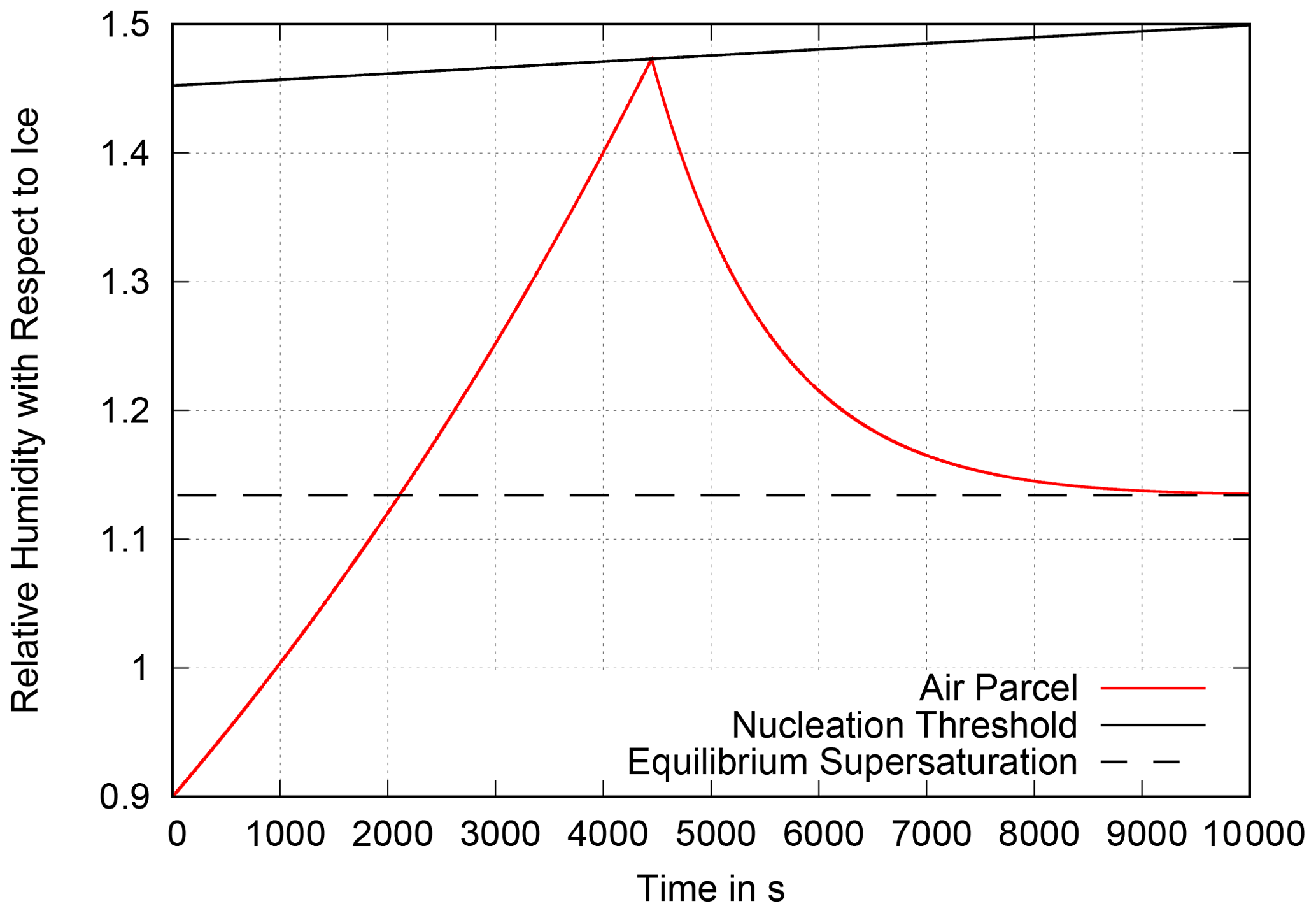
Figure 1Example of the cooling-cloud formation-phase relaxation process. The red curve shows the supersaturation of a single air parcel as it increases over time, until it reaches the nucleation threshold (solid black line). From there on, the supersaturation is consumed by depositional growth of ice crystals, which lowers the supersaturation down to an equilibrium value (dashed black line) a few percent above saturation.
As the cloudy air parcels had their individual nucleation events at different times, their current supersaturation is spread over a certain range of values with a distribution that needs to be determined. In principle, this can be achieved using the box model and making a histogram of the supersaturation values. For more complicated initial conditions than assumed here, this might actually be necessary; however, as we start from a uniform distribution of qp in the clear grid box (which is equivalent to a uniform distribution of the relative humidity at constant T throughout the box, as assumed), one can derive an analytical expression for the supersaturation distribution in the cloudy air parcels, . At the moment of nucleation, the air parcel has a supersaturation Snuc; thereafter, the supersaturation will approach the mentioned equilibrium value, Seq. As temperature changes little during a small time step, the change in Seq is generally negligible and the corresponding change in Snuc is small (see Fig. 1). We neglect these changes for simplicity. We rather assume that, for a little while after nucleation, the supersaturation, s, in a single air parcel evolves as follows:
This means that the growing cloud always consists of young, highly supersaturated parts and old parts with a supersaturation close to the current Seq. After some time has passed, the corresponding humidity distribution within the cloud appears to be of hyperbolic shape with high probability densities close to Seq and lower densities at higher supersaturation. In order to derive , we start from the corresponding distribution of individual nucleation times, which is approximately a uniform one due to the assumption of an initially uniform distribution of qp and a constant cooling rate during one time step. Let, as before, nucleation start at a time t0 and let us consider the situation at a later time t1, which is either within the same time step or the end of the current time step. Then, the uniform distribution of nucleation times is as follows:
We now use the transformation law for probability densities to derive from . Using Eq. (12) gives the relation between Sp and tnuc,
from which we calculate the derivative,
With this, the transformation law reads
and the desired result is
where
Figure 2 shows that, despite the assumptions made, this analytical solution closely captures the probability distribution generated by the model.
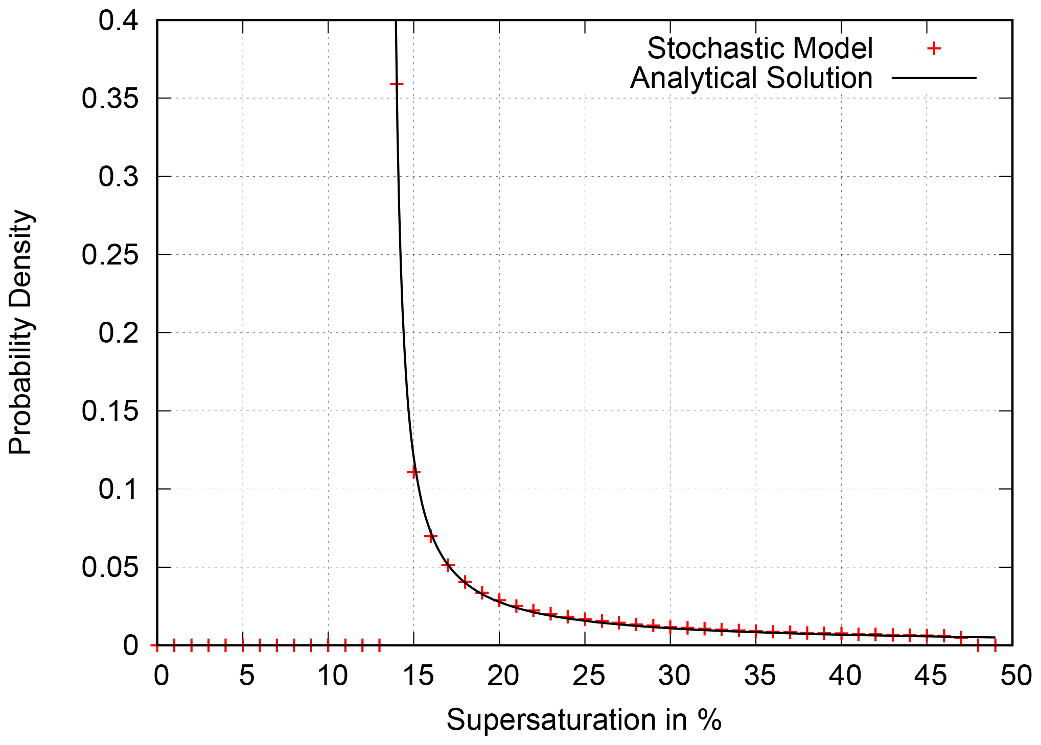
Figure 2Hyperbolic distribution of supersaturation in the cloudy part of a grid box, analytical solution (solid line) and numerical result.
With S0 and S1, one can write the distribution of supersaturation within the cloudy air parcels in terms of supersaturation values alone:
Note that, later, after nucleation has stopped, S1 will no longer be Snuc; instead, it will evolve according to Eq. (12), with , but the general expression for the hyperbolic distribution of Sp will still be valid.
It is easy to see that, for large times t1, the distribution of in-cloud supersaturation approaches a delta distribution centred at the equilibrium supersaturation:
This end point is higher than saturation as long as there is cooling, and this is an important difference to saturation adjustment.
2.2 New parameterisation
We propose a new, simple ice-cloud scheme that overcomes saturation adjustment by directly modelling the decay of supersaturation once cloud formation has begun at temperatures below the supercooling limit for small droplets at about −38 ∘C. For this purpose, again consider a single model grid box with temperature T, specific humidity q, cloud fraction C and specific ice water content qi. Further, let δT be the change in T when integrating the next model time step and again imagine the grid box to consist of an arbitrarily large number of air parcels.
2.2.1 Initial cloud formation
Let us first consider δT<0 and C=0; thus, qi=0. In this case, we again assume qp to be uniformly distributed between qlow and qhigh across the grid box. As T decreases, qs(T) and qnuc(T) drop as well, and cloud formation is initiated if qnuc(T) passes qp at one point within the grid box. According to the sub-grid humidity fluctuations, this happens if qnuc<qhigh at the end of the current time step or, equivalently, if
where the upper indices n, n+1 label time steps in the following. The duration of one time step is .
Consistent with the assumption of uniform q fluctuations, the time, t0, of the first air parcel becoming cloudy and the cloud fraction at the end of the time step can both be determined by simple geometric (i.e. linear) considerations. Assuming that qnuc decreases linearly with time during a time step gives the following:
Similarly, we calculate the cloud fraction for the next time step as the difference between qhigh and divided by the total spread in qp:
With t0 and the humidity distribution from Eq. (17) inside the new cloud, we can calculate the mean relative supersaturation Scl inside the cloud at tn+1.
We leave it open here at which moment within a time step the quantities Snuc and Seq are evaluated. The choice does not have much effect, as these quantities vary little over one time step. In our simulations, we always use the values at the beginning of the time step. The two limits of Eq. (24) are Seq for large time differences and Snuc for very small time differences, as expected. Note that we introduce qcl as a new prognostic variable at this point. This appears to be necessary in order to overcome saturation adjustment entirely.
The mean specific humidity in the clear air right after cloud formation, , can be determined with a geometric consideration as well. Before cloud formation, the total spread in specific humidity was . After partial cloud formation, this spread is reduced by a factor , such that
Figure 3 shows schematically how the clear-sky humidity develops over time.
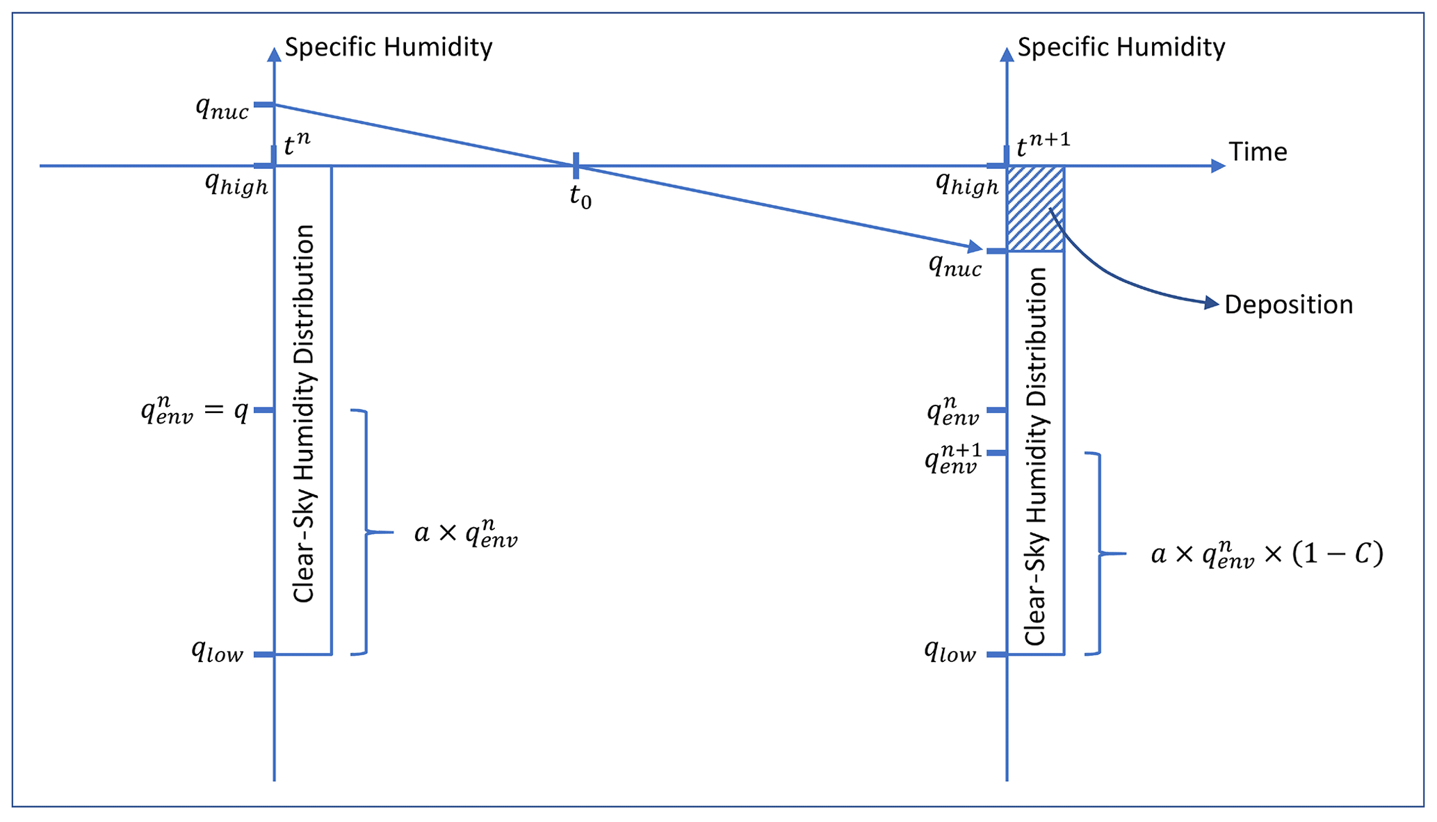
Figure 3Schematic on the initiation of cloud formation in the parameterisation. At the time t0, qnuc propagates into the clear-sky humidity distribution, thereby causing nucleation in the moistest part of the grid box. The parameterisation turns this part into a cloud, and qnuc becomes the new top end of the clear-sky humidity distribution. The mean clear-sky humidity qenv is adjusted accordingly.
If cloud formation was so vigorous (or if the grid box was small with small a) that the cloud fraction became unity within the time step, would be undefined and the mean specific humidity in the grid box, q, would correspond to the mean supersaturation in the cloud. Otherwise, the mean specific humidity is the weighted mean of and :
For the mean specific ice water content , we know that all water vapour that leaves the gas phase is deposited as ice; thus,
Note that these equations are valid at the end of the time step at which cloud formation commences. Equations for later time steps will be derived below.
2.2.2 Continual cloud growth
Let us now consider further time steps in which cloud formation continues and the cloud fraction increases. The general time step ranges from tn+i to , where i≥1, but let us take i=1 for simplicity of notation. We now use our new prognostic variable qcl to recover the mean specific humidity in the clear-sky part of the grid box by rearranging Eq. (27):
It is necessary to formulate all changes in terms of quantities at the two considered time steps, so that not too many quantities have to be kept in memory. Again, determining the new cloud fraction, Cn+2, is a simple geometric task and the result is as follows:
With this, the new average specific humidity in the cloud-free part, , can be computed in analogy to Eq. (26):
but it is necessary to replace by its updated value from Eq. (26) here, giving
For the in-cloud humidity, we split the grown cloud into the old part with cloud fraction Cn+1 and the new part with cloud fraction . In the new part, cloud formation is initiated as before according to Eqs. (24)–(25), but now nucleation occurs right from the beginning of the time step, giving the following:
The old cloud part, on the other hand, can be considered to be an individual cloud that stopped growing at tn+1. If a cloud stops growing, not only the lower boundary S0 of the in-cloud distribution of supersaturation further approaches Seq but the upper boundary S1 also starts to deviate from Snuc, as mentioned above. Both boundaries develop in a similar way; the lower one proceeds further as in Eq. (18), with the end time updated. The upper one proceeds in an analogous way, however, with t0 replaced by tn+1. In this case, we have the following:
In order to evaluate this, one would need to have t0 still in memory. Instead, we recognise that this is a simple exponential decay towards Seq, as we would expect if qp decays exponentially in all of the air parcels. Thus, the specific humidity qold in the old cloud part can simply be calculated as follows:
Putting the cloud together again, we can derive the following:
Figure 4 shows schematically how the in-cloud humidity develops over time.
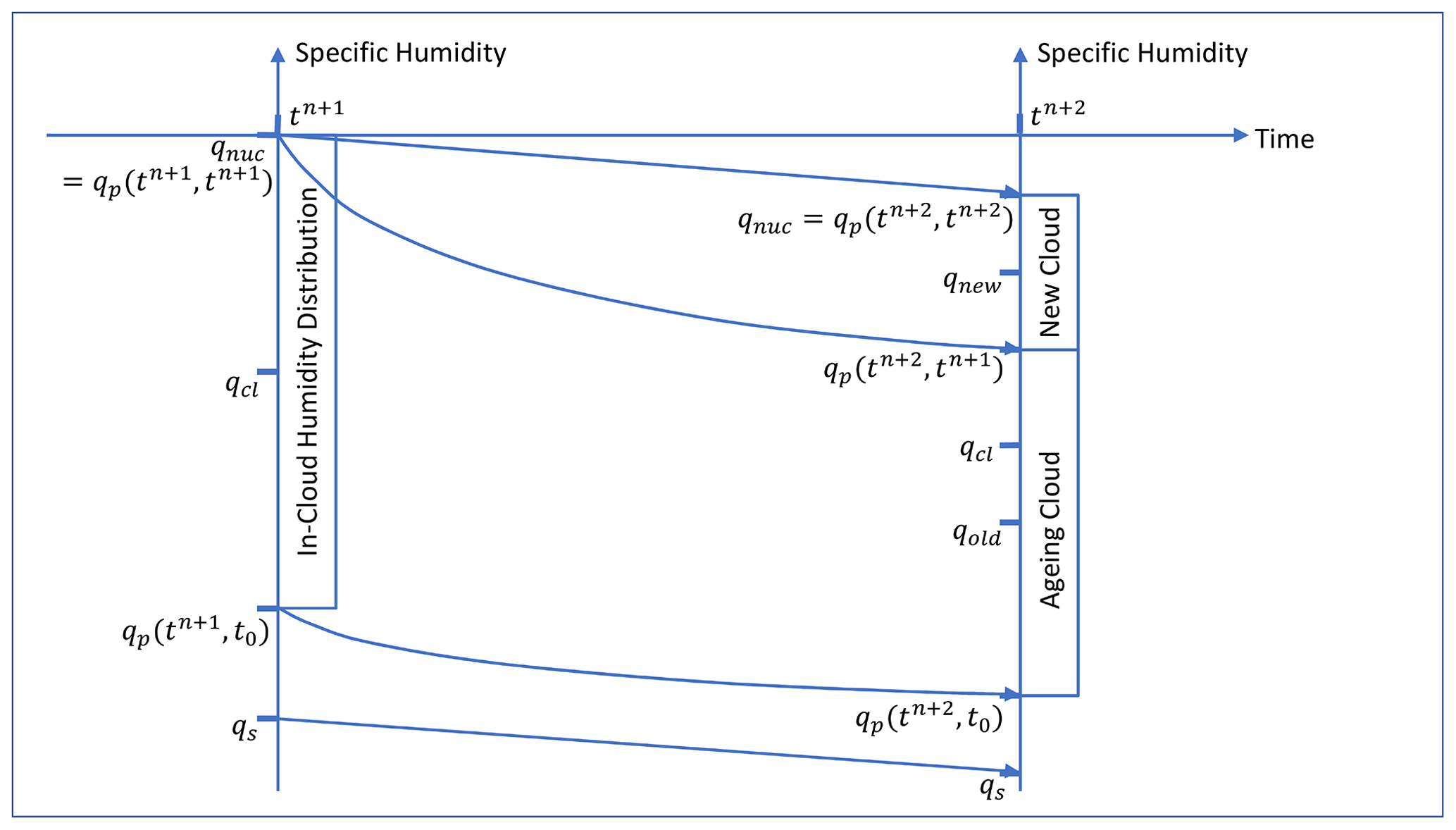
Figure 4Schematic of the evolution of the in-cloud humidity during ongoing cloud formation. The boundaries of the humidity distribution in the already existing cloud decay exponentially towards qs, while the steady decrease in qnuc continuously causes nucleation in further parts of the clear-sky portion of the grid box. These new cloud parts begin their own decay towards qs at their individual nucleation times, resulting in a steady new humidity distribution in the grown cloud with the new qnuc as its top end.
The mean specific humidity in the grid box, qn+2, is (as before) the weighted mean of and , and the new specific ice water content is given by the following:
2.2.3 Continual cloud growth to full coverage
If full cloud coverage is reached within a time step, it is necessary to record the point in time, t1, when this happens. This can again be done by a geometric consideration. Let the current time step start at tm. The current clear-sky specific humidity can again be calculated according to Eq. (29). With this, t1 becomes
Now one computes the average supersaturation in the new cloud part at tm+1 in two steps. The first step ranges from tm to t1, for which the upper boundary of is still the current nucleation threshold. This gives a preliminary supersaturation, :
The equilibrium and nucleation supersaturations have to be taken at the conditions of the current time step. After nucleation has ceased – that is, in the second step from t1 to tm+1 – the new cloud part can be treated like the old one:
The specific humidity in the old cloud part can be calculated as before, such that we have the following for qm+1:
Cm+1 can then be set to 1 and can be calculated as before.
2.2.4 Completely covered sky and cooling
Let us now consider a time step tm+i to after full coverage has been reached, where we again take i=1 for simplicity of notation. In this simple case, we only let q decay further towards qs, while qs itself decreases:
We calculate analogously to Eq. (38).
2.2.5 Warming a cloud
Now consider a time step tk to tk+1, during which there is a cloud inside the grid box and δT>0. If the grid box mean temperature keeps rising over a longer period of time, the ice crystals inside the cloud are expected to return to the gas phase and eventually vanish. During this process, it is hard to determine a threshold for qi,p below which a specific air parcel can be considered to be no longer cloudy. As we also neglect cloud edge erosion in this concept, we simply do not let any air parcel leave the cloud and keep C constant until all ice has sublimated.
For the in-cloud humidity, we again have the conditions of a cloud that is no longer growing, i.e. Scl decays exponentially towards Seq. Therefore, qcl evolves analogously to Eq. (44):
qk+1 and can then be calculated via the following expressions:
If , the cloud is about to vanish in the course of the current time step. In this case, we instead simply set the following:
The new parameterisation has been tested against the stochastic box model and against a parameterisation with saturation adjustment in various scenarios of cloud formation and dissolution, which are essentially distinguished by the temporal behaviour of the vertical velocity, w(t), or, equivalently, of the adiabatic cooling and warming over time. Two such scenarios are considered: one with a constant updraught and one where w(t) follows a cosine function with two different amplitudes (see Fig. 5a). These two scenarios are additionally combined with variations in the other parameters (i.e. α, a and Δt) in order to test the sensitivity of the parameterisation to variations in these parameters. Table 1 gives an overview of the performed simulations. Figure 5b provides an example of how the cloud fraction evolves in the two wind scenarios with the parameter settings of the first two simulations.
Table 1Overview of the tests. The scenarios are characterised by either a constant updraught velocity (“const” in the second column) or a variable one characterised by a pair of cosine functions (“cos”) (see Fig. 5a).
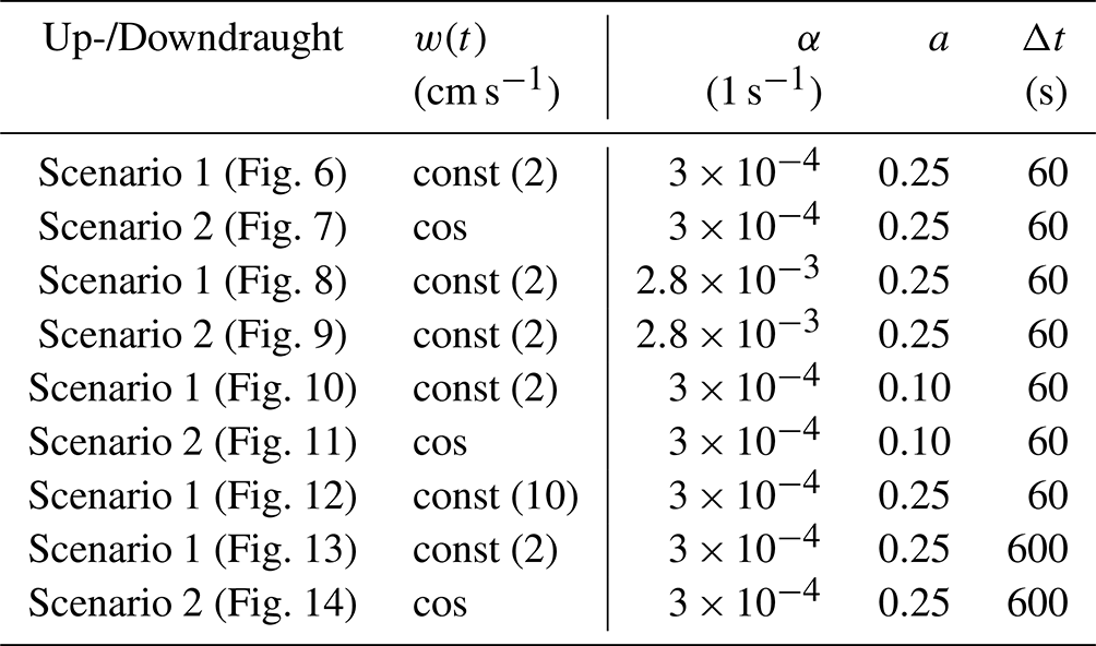
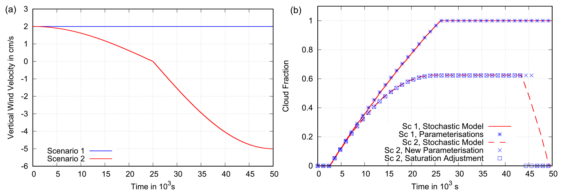
Figure 5Panel (a) presents a visualisation of the considered vertical wind speed scenarios. Scenario 1 is characterised by a constant updraught, whereas the vertical wind speed in Scenario 2 follows half a period of a cosine function in time with an increase in amplitude halfway through the simulation from 2 to 5 cm s−1. Panel (b) shows the corresponding evolutions of the cloud fraction in the stochastic model and the parameterisations for s−1 and a=0.25. As can be seen, the parameterisations both capture the evolution of the cloud fraction precisely. Only the process of cloud dissolution is not modelled accurately, as the cloud fraction is simply set to zero once all ice has sublimated. Note that the sublimation process is slower in the new parameterisation compared with the one using saturation adjustment, thereby increasing the cloud lifetime.
All tests are illustrated using pairs of figures: each left panel shows the temporal evolution of the grid-mean relative humidity, which is an output variable of NWP models, and each right panel shows the temporal evolution of the in-cloud relative humidity, which is (proportional to) the new prognostic variable in our concept. All simulations start from an initial grid box mean temperature of 235 K so that the temperature at the time of first nucleation will always be below the threshold for homogeneous freezing.
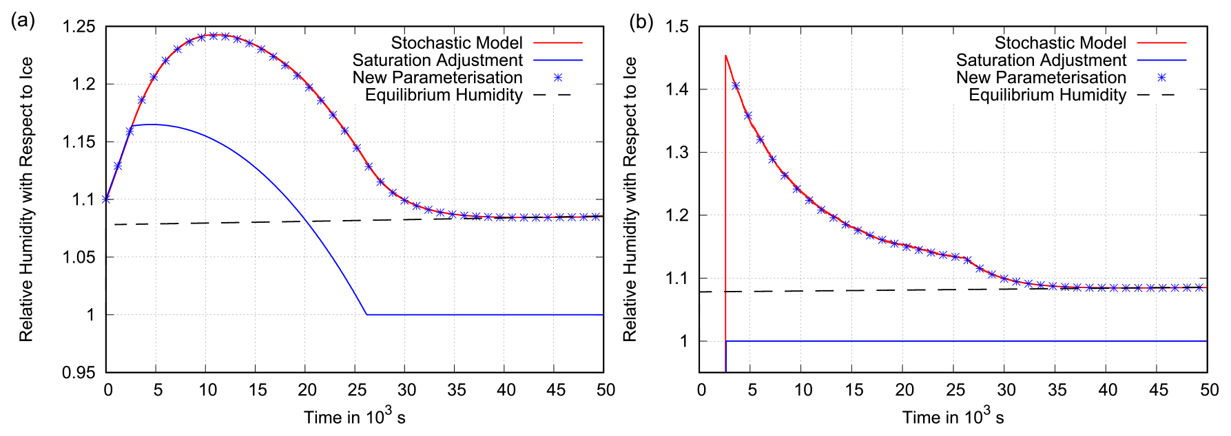
Figure 6Scenario 1. Panel (a) shows the grid box mean relative humidity (with respect to ice) as a function of time in a grid box with a=0.25 that undergoes cooling in a constant updraught of 2 cm s−1 and cloud formation with s−1. Shown is the behaviour of the stochastic box model that treats one grid box as an ensemble of 104 air parcels with an initial distribution of specific humidity (red line); this model is assumed to best represent reality and serves as a benchmark for the parameterisations. The new parameterisation (blue stars) follows the stochastic model closely, while the parameterisation that uses saturation adjustment does not, leading to an underestimation of the mean relative humidity and, thus, of supersaturation. The new parameterisation approaches the equilibrium supersaturation (dashed black line), while saturation adjustment assumes exactly saturated conditions inside the cloud. Panel (b) presents the corresponding mean in-cloud relative humidity for the stochastic model, the new parameterisation and the parameterisation with saturation adjustment. One can clearly see how the decay of humidity in the stochastic box model changes into a pure exponential decay once the cloud fraction reaches unity and no new, highly supersaturated cloud parts join the cloud anymore (see Fig. 5b).
The first simulation uses a constant uplift speed of 2 cm s−1 and ice growth with s−1. The value of α is chosen by taking the results of Khvorostyanov and Sassen (1998b) into account. According to their Table A1, this value would be appropriate, for example, if about 100 ice crystals with a mean radius of 10 µm were present per litre of air. We set a=0.25, such that nucleation is initiated once , which is the current standard in the Integrated Forecast System. The time step is 60 s. Figure 6 illustrates two mechanisms of how saturation adjustment leads to an underestimation of supersaturation in cloudy situations. Right from the initiation of cloud formation in a grid box, saturation adjustment drives the mean relative humidity over ice down to 100 %. As soon as full cloud coverage is reached, the mean relative humidity is and stays at 100 %. On the contrary, the stochastic box model (which is our benchmark) shows that the humidity still increases after cloud initiation, reaches a maximum and then approaches the equilibrium supersaturation a few percent above 100 %. The new parameterisation closely follows this behaviour and, thus, represents reality better than saturation adjustment. The two reasons for the underestimation of supersaturation in the current parameterisations with saturation adjustment are (1) a decrease in supersaturation right at cloud initiation and (2) ignorance of the equilibrium supersaturation later. This becomes particularly evident in Fig. 6b, where the in-cloud relative humidity is plotted for this case. With saturation adjustment, there is no in-cloud supersaturation; however, in reality, there is in-cloud supersaturation at least as long as cooling proceeds.
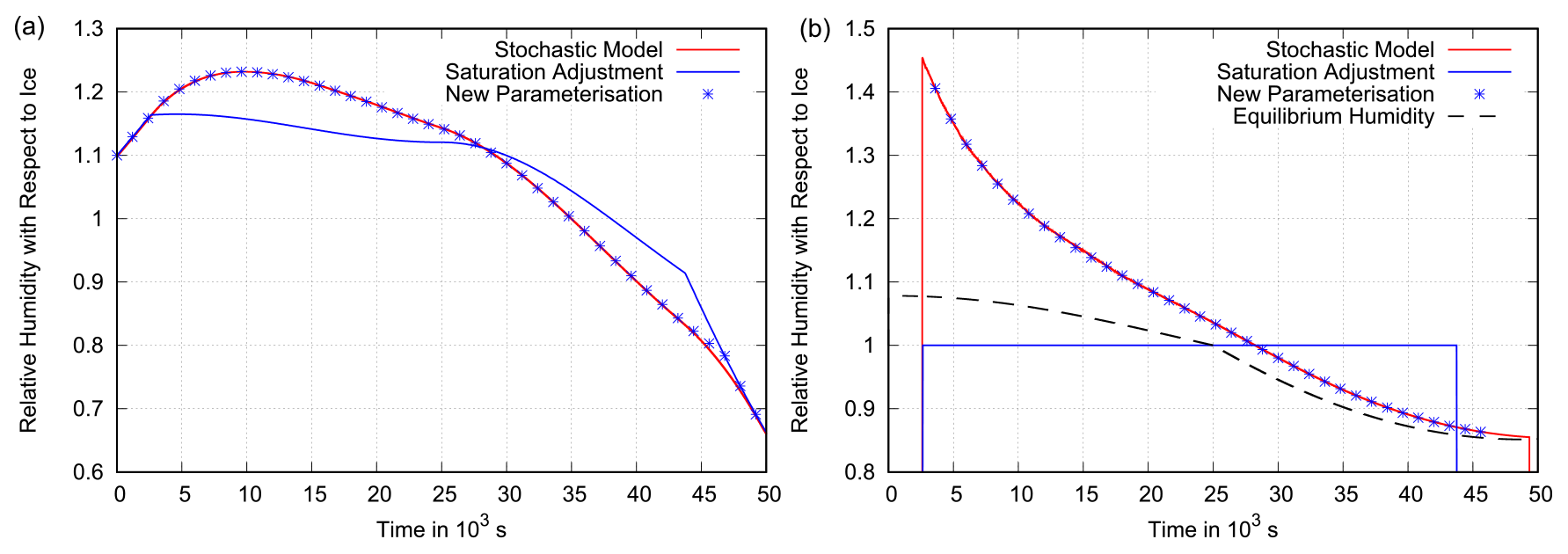
Figure 7Scenario 2. Panel (a) shows the grid box mean relative humidity (with respect to ice) as a function of time in an updraught with an initial speed of 2 cm s−1 that weakens over time and becomes a downdraught accelerating to 5 cm s−1 (see Fig. 5). Other simulation parameters are s−1 and a=0.25. The behaviour of the benchmark box model is shown in red. The new parameterisation (blue stars) follows the benchmark simulation closely, while the parameterisation that uses saturation adjustment does not, leading to an underestimation of relative humidity during the cooling period and an overestimation during the warming period. Panel (b) presents the corresponding mean in-cloud relative humidity for the stochastic model, the new parameterisation and the parameterisation with saturation adjustment. The box model and the new parameterisation approach the equilibrium supersaturation (dashed black line), while saturation adjustment assumes exactly saturated conditions inside the cloud.
The second test is a situation in which the cooling rate follows a cosine function that changes amplitude halfway through the simulation: the simulation starts with cooling through an updraught of 2 cm s−1 that gets weaker over time and reverses into warming and ice sublimation in a final downdraught of 5 cm s−1. The temporal evolution of relative humidity (grid box average and in-cloud average) is shown in Fig. 7. Clearly, saturation adjustment also shows a deviating behaviour under the warming conditions in the second half of the simulation. In the stochastic box model and the new parameterisation, the in-cloud RHi approaches the equilibrium humidity, which is now below saturation, while the cloud again is assumed to be exactly saturated in the model with saturation adjustment. Sublimation is (just as deposition) only effective if the relative humidity deviates from saturation, and it is not an instantaneous process in reality. Therefore, subsaturation inside the cloud can be considered the more realistic state; hence, the new parameterisation shows an improvement to saturation adjustment also under warming conditions.
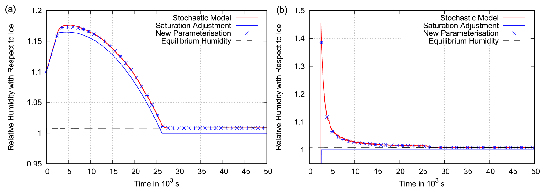
Figure 8Scenario 1. Panel (a) shows the grid box mean relative humidity (with respect to ice) as a function of time in a constant updraught of 2 cm s−1 with a=0.25. The assumed deposition rate is high, s−1, which corresponds to a cloud with 1000 crystals of 10 µm radius per litre. The behaviour of the benchmark box model is shown in red. The new parameterisation (blue stars) follows the benchmark simulation closely, while the parameterisation that uses saturation adjustment does not. This leads to only a slight underestimation of relative humidity due to the large deposition rate. Panel (b) presents the corresponding mean in-cloud relative humidity for the stochastic model, the new parameterisation and the parameterisation with saturation adjustment. The box model and the new parameterisation approach the equilibrium supersaturation (dashed black line), while saturation adjustment assumes exactly saturation inside the cloud.
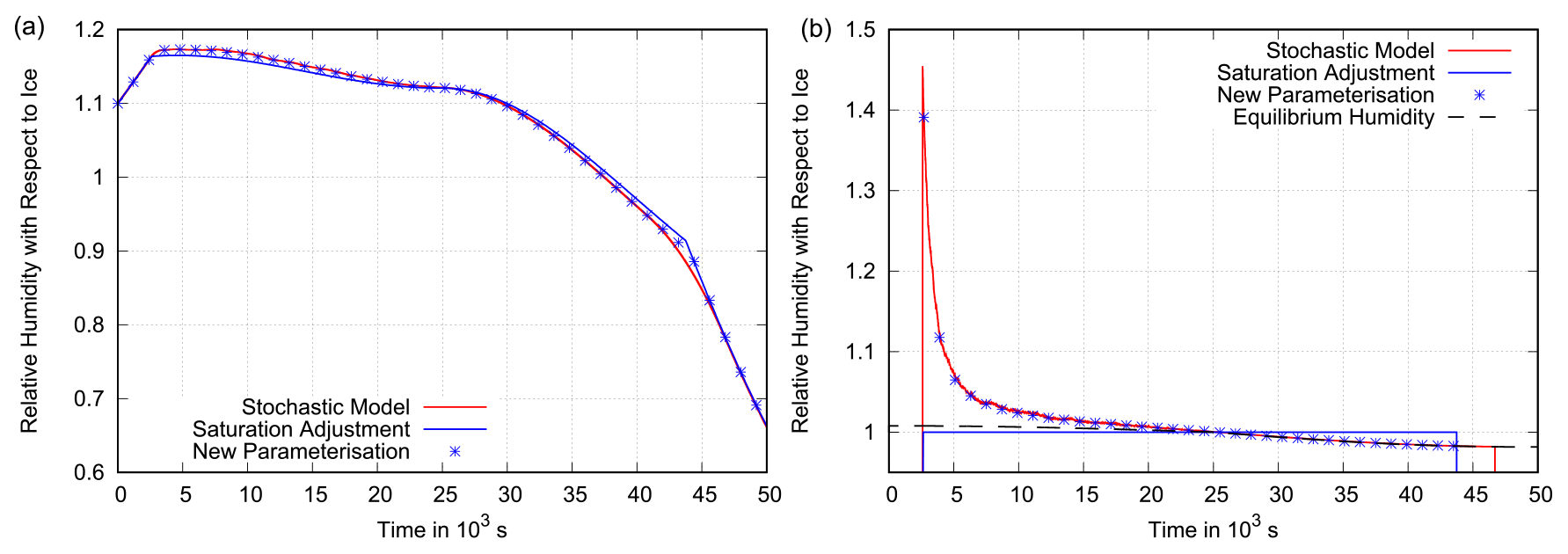
Figure 9Scenario 2. Panel (a) shows the grid box mean relative humidity (with respect to ice) as a function of time with a=0.25 in an updraught with an initial speed of 2 cm s−1 that weakens over time and becomes a downdraught accelerating to 5 cm s−1 (see Fig. 5). The assumed deposition rate is high, s−1, which corresponds to a cloud with 1000 crystals of 10 µm radius per litre. The behaviour of the benchmark box model is shown in red and is closely followed by the new parameterisation (blue stars). The parameterisation that uses saturation adjustment only slightly underestimates relative humidity during the cooling period and slightly overestimates it during the warming period due to the large deposition rate. Panel (b) presents the corresponding mean in-cloud relative humidity for the stochastic model, the new parameterisation and the parameterisation with saturation adjustment. The box model and the new parameterisation approach the equilibrium supersaturation (dashed black line), while saturation adjustment assumes exactly saturated conditions inside the cloud.
Next, cases with a higher ice formation rate of s−1 are considered, which corresponds to clouds with 1000 ice crystals of 10 µm radius per litre. The corresponding phase relaxation time is only 6 min. Figures 8 and 9 show that quite small differences between the old and the new parameterisation and the stochastic box model remain if the in-cloud supersaturation is consumed quickly, as expected. Of course, right after cloud formation, there is considerable supersaturation in the cloud which is not at all represented by the old parameterisation (Figs. 8b, 9b); however, as the cloud fraction is initially small, this does not cause a large difference in the mean specific humidity (see Figs. 8a, 9a). Thus, saturation adjustment leads to only a small underestimation of supersaturation in cases of clouds with quick vapour deposition on ice.
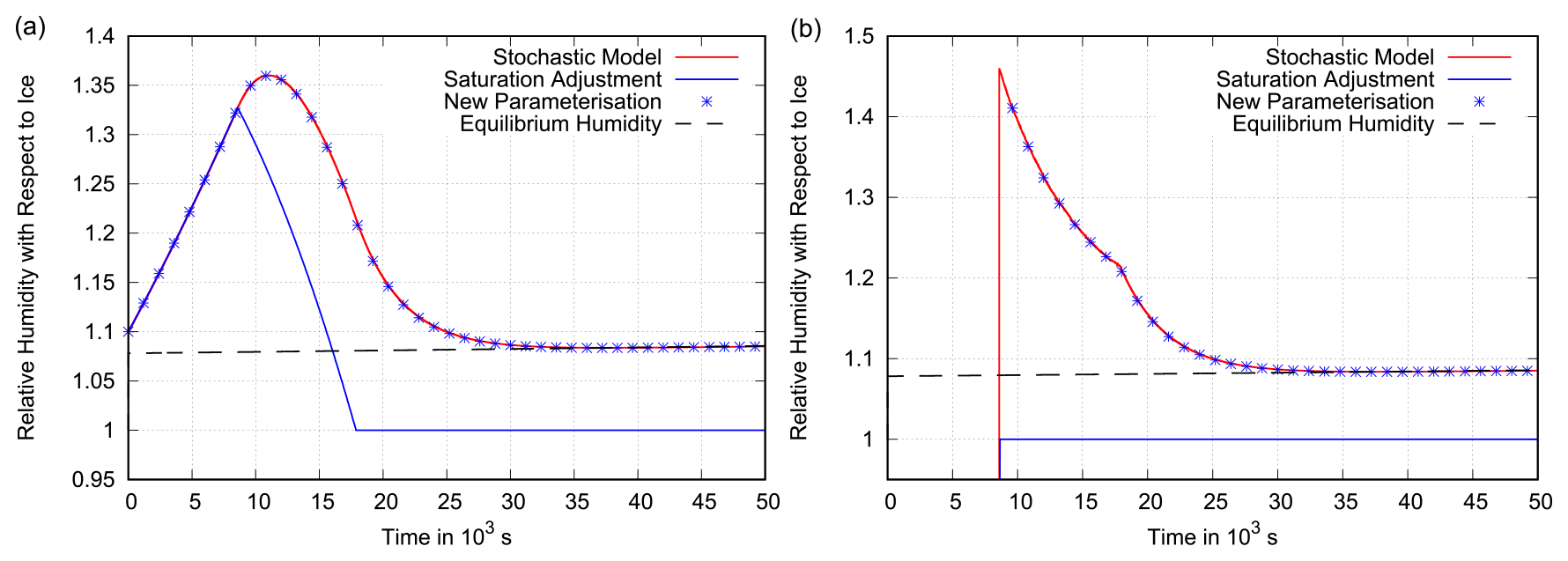
Figure 10Scenario 1. Panel (a) shows the grid box mean relative humidity (with respect to ice) as a function of time in a constant updraught of 2 cm s−1. The assumed deposition rate is s−1. The initial humidity distribution is narrow with a=0.1. The behaviour of the benchmark box model is shown in red. The new parameterisation (blue stars) follows the benchmark simulation closely, while the parameterisation that uses saturation adjustment does not, leading to a larger underestimation of relative humidity compared with the reference simulation in Fig. 6. Panel (b) presents the corresponding mean in-cloud relative humidity for the stochastic model, the new parameterisation and the parameterisation with saturation adjustment. The box model and the new parameterisation approach the equilibrium supersaturation (dashed black line), while saturation adjustment assumes exactly saturation inside the cloud.
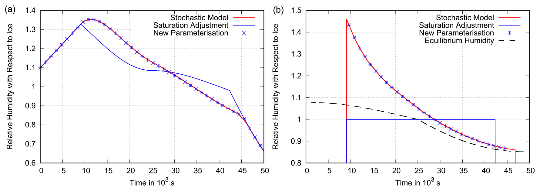
Figure 11Scenario 2. Panel (a) shows the grid box mean relative humidity (with respect to ice) as a function of time in an updraught with an initial speed of 2 cm s−1 that weakens over time and becomes a downdraught accelerating to 5 cm s−1 (see Fig. 5). The assumed deposition rate is s−1. The initial humidity distribution is narrow with a=0.1. The behaviour of the benchmark box model is shown in red and is closely followed by the new parameterisation (blue stars). The parameterisation that uses saturation adjustment underestimates relative humidity during the cooling period and overestimates it during the warming period more strongly due to the narrower clear-sky humidity distribution. Panel (b) presents the corresponding mean in-cloud relative humidity for the stochastic model, the new parameterisation and the parameterisation with saturation adjustment. The box model and the new parameterisation approach the equilibrium supersaturation (dashed black line), while saturation adjustment assumes exactly saturated conditions inside the cloud.
As the results of Gierens et al. (2007) suggest, the actual spread in q across a small model grid box (i.e. higher resolution) is probably smaller than ±25 %. Figures 10 and 11 show that the deviation of the parameterisation with saturation adjustment from the stochastic box model increases in a case with a narrower initial distribution of q (here ±10 %). The maximum deviation in the constant updraught simulation increases from less than 15 percentage points in Fig. 6 to about 20 percentage points in Fig. 10, and the maximum deviation in the modulated updraught simulation increases from less than 10 percentage points (Fig. 7) to more than 10 points (Fig. 11). The reason is that the cloud fraction increases faster if the spread in q is smaller. Thus, the initially high supersaturation inside the cloud in the stochastic box model gains more weight in the grid box mean relative humidity, whereas saturation adjustment drives the grid box mean relative humidity back to 100 % even faster.
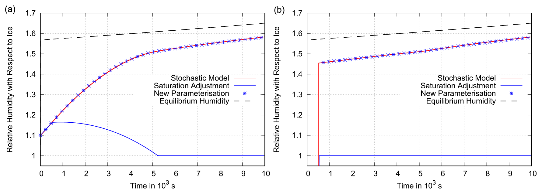
Figure 12Scenario 1. Panel (a) shows the grid box mean relative humidity (with respect to ice) as a function of time in a fast constant updraught of 10 cm s−1. Other simulation parameters are s−1 and a=0.25. The behaviour of the benchmark box model is shown in red. It increases steadily and is closely followed by the new parameterisation (blue stars), while the parameterisation that uses saturation adjustment does not even reproduce the same trend. Hence, in principle, the new parameterisation is capable of simulating large supersaturations beyond the threshold for homogeneous nucleation occasionally found in the real atmosphere. However, the box model result quickly becomes unrealistic, as the increasing supersaturation would cause α to grow due to a rapid increase in crystal number density. Panel (b) presents the corresponding mean in-cloud relative humidity for the stochastic model, the new parameterisation and the parameterisation with saturation adjustment. The box model and the new parameterisation approach the equilibrium supersaturation (dashed black line), while saturation adjustment assumes exactly saturated conditions inside the cloud.
The equilibrium supersaturation rises quickly with increasing cooling rates. Figure 12 shows that it can even rise beyond the nucleation threshold in a rather extreme case with a 10 cm s−1 constant updraught. In such a situation, the deposition of water vapour on the ice crystals is not fast enough to make the supersaturation inside the cloud decay; it can only slow down the further increase. Here, saturation adjustment not only leads to incorrect grid box mean relative humidity values but also to an incorrect trend. In any case, this simulation soon becomes unrealistic, as the high supersaturation would let the ice crystals grow quickly in size and number. Thus, the available surface for vapour deposition would increase and the value of α would grow larger and larger. Hence, the equilibrium supersaturation would soon decrease again and the state of steadily increasing supersaturation could no longer be maintained.
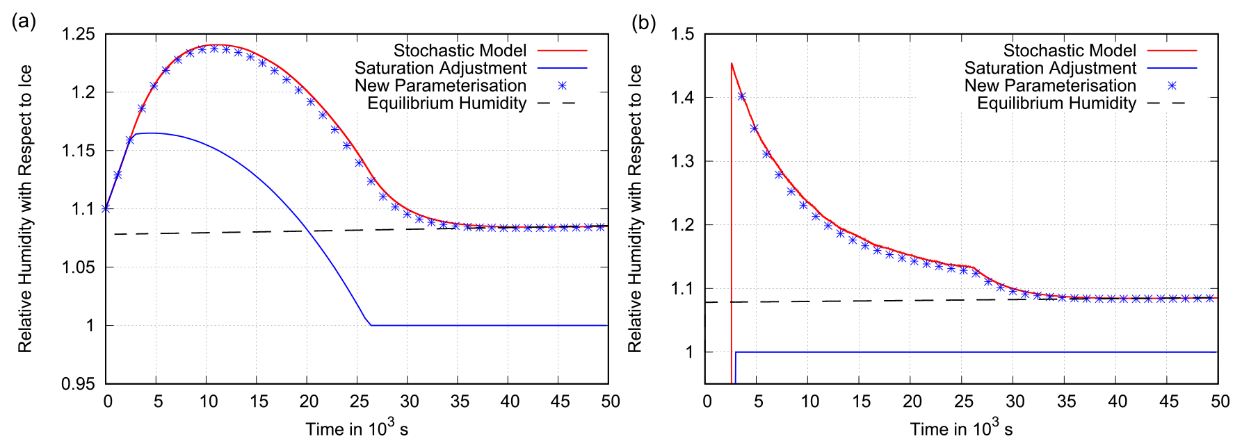
Figure 13Scenario 1. Panel (a) shows the grid box mean relative humidity (with respect to ice) as a function of time in a constant updraught of 2 cm s−1. Other simulation parameters are s−1 and a=0.25. The time step of the parameterisations is increased to 10 min. The behaviour of the benchmark box model is shown in red. The new parameterisation (blue stars) still follows the benchmark simulation quite closely, while the parameterisation that uses saturation adjustment does not, leading to an underestimation of relative humidity. Panel (b) presents the corresponding mean in-cloud relative humidity for the stochastic model, the new parameterisation and the parameterisation with saturation adjustment. The box model and the new parameterisation approach the equilibrium supersaturation (dashed black line), while saturation adjustment assumes exactly saturation inside the cloud.
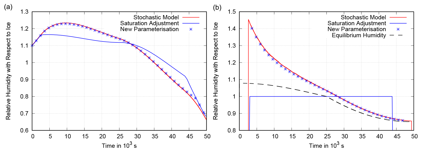
Figure 14Scenario 2. Panel (a) shows the grid box mean relative humidity (with respect to ice) as a function of time in an updraught with an initial speed of 2 cm s−1 that weakens over time and becomes a downdraught accelerating to 5 cm s−1 (see Fig. 5). Other simulation parameters are s−1 and a=0.25. The time step of the parameterisations is increased to 10 min. The behaviour of the benchmark box model is shown in red and is still closely followed by the new parameterisation (blue stars). The parameterisation that uses saturation adjustment underestimates relative humidity during the cooling period and overestimates it during the warming period. Panel (b) presents the corresponding mean in-cloud relative humidity for the stochastic model, the new parameterisation and the parameterisation with saturation adjustment. The box model and the new parameterisation approach the equilibrium supersaturation (dashed black line), while saturation adjustment assumes exactly saturated conditions inside the cloud.
A time step of 1 min is rather short in NWP. Therefore, we also test the sensitivity of the new parameterisation to the length of the time step by repeating the two experiments with a time step of 10 min. The results are shown in Figs. 13 and 14. Comparing these figures to Figs. 6 and 7, one can clearly see that the sensitivity is low. The new parameterisation still precisely captures the onset of cloud formation and also later closely follows the behaviour of the stochastic box model. The slight deviation by the end of the modulated cooling simulation (Fig. 14a) is not due to an error in the specific humidity, as the three models show identical final values in a plot of specific humidity (not shown). This deviation in relative humidity is rather due to the rough approximation of the time dependence of the updraught resulting in a deviation in temperature. Finally, the time step was increased to 30 min and the deviation of the new parameterisation from the stochastic box model was still small (not shown).
Overall, the new parameterisation always stayed close to the stochastic box model in all performed tests and, thus, has proven to be numerically stable against variations in all considered parameters.
It is important to see that saturation adjustment is a special case of the new parameterisation, namely one with a very large value of the deposition rate α (or equivalently a very short phase relaxation time). Our first sensitivity study (Figs. 8, 9) has shown that both parameterisations give more similar results if the phase relaxation time is short. Equation (11) shows that the equilibrium supersaturation approaches zero (i.e. the relative humidity over ice approaches 100 %) when α becomes very large. Thus, both causes for the underestimation of supersaturation vanish in this limit. However, this limit is not the typical case for cirrus clouds.
One can estimate a value for α as the reciprocal value of the phase relaxation time given by Khvorostyanov and Sassen (1998a):
where D is the temperature- and pressure-dependent water vapour diffusion coefficient, N is the number concentration of ice crystals, and is the radius that they would obtain if the complete excess vapour was transferred into N spherical crystals. In this equation, the diffusion coefficient has the smallest variability (Pruppacher and Klett, 1997), while the number density and crystal radius vary over several orders of magnitude (Dowling and Radke, 1990; Heymsfield et al., 2017; Krämer et al., 2009, 2016, 2020). The data in these papers indicate that short relaxation times (high N and large crystals) are typical of liquid-origin cirrus, while cirrus formed in situ is rather characterised by longer relaxation times; thus, we can expect long-lasting in-cloud supersaturation in this kind of cirrus. In contrast, liquid-origin cirrus is characterised by its liquid origin (i.e. it started from water saturation), which implies high ice supersaturation that relaxes to ice saturation quickly.
In the tests described above, we kept the value of α constant throughout each simulation. This is similar to the approach with saturation adjustment, where, although α is not specified, we can conceive it as a constant very large value. However, a constant α is not a condition for the new parameterisation, and we plan to recalculate it every time step for every grid box based on the individual meteorological conditions influencing the quantities in Eq. (52) when implementing the parameterisation into an actual 3D-NWP model. Firstly, N can be estimated via the updraught speed, w, when the cloud forms, using the relation from Kärcher and Lohmann (2002). This relation only holds for clear air, and a lower number density has to be assumed if pre-existing ice is present. Secondly, can be estimated by assuming that the supersaturation is completely transferred to spherical ice crystals with radius . In a further test with the stochastic box model, we let α vary with for every air parcel. For this test, we also introduced uniformly distributed, random sub-grid fluctuations in w of ±1 cm s−1 to investigate how small-scale updraught fluctuations affect the nucleation rate. Therefore, every second each air parcel experienced a new random updraught of between 1 and 3 cm s−1. Figure 15 shows that the updraught fluctuations result in an overall higher mean value of α, leading to a slightly lower relative humidity shortly after the onset of nucleation. However, the non-linear dependence of Seq on α and causes an increase in the equilibrium supersaturation, thereby leading to an increased relative humidity in the aged cloud. Overall, the two simulations do not differ very much; this provides hope that the negligence of updraught fluctuations and the use of a single value for α do not introduce large errors into simulations of the new parameterisation.
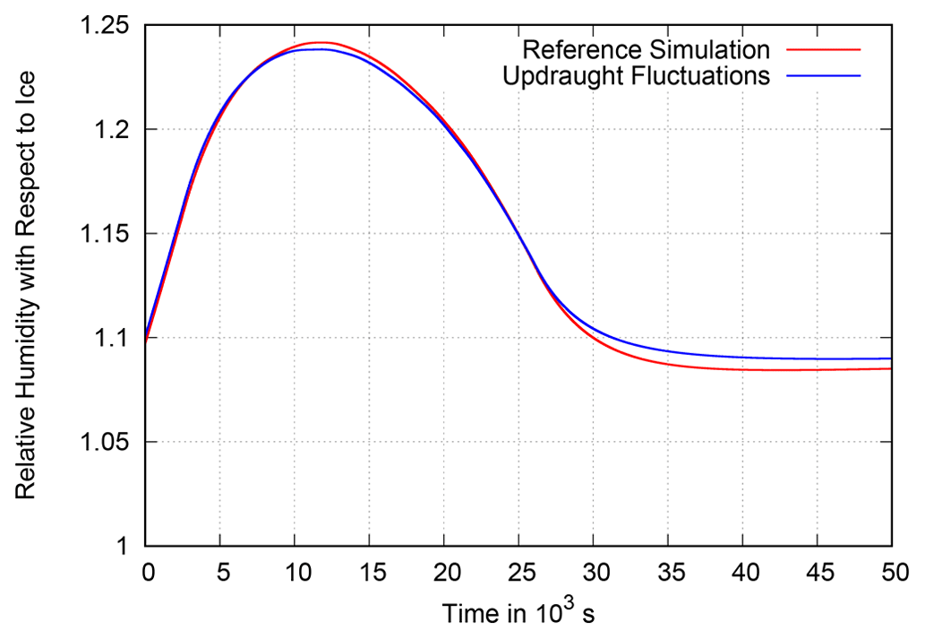
Figure 15Evolution of the grid box mean relative humidity in the stochastic box model in a simulation in which each air parcel experiences a random updraught of between 1 and 3 cm s−1 (blue) every time step. α varies with the updraught velocity at the time of nucleation in the individual air parcel around s−1. The red plot shows the reference simulation of the stochastic box model from Fig. 6 with uniform w=2 cm s−1 and uniform s−1 for all air parcels. Even though the updraught fluctuations cause a slightly larger mean value of α, they lead to an increased equilibrium humidity in the aged cloud due to the non-linear dependence of Seq on .
Another process that has been simplified is nucleation. On the one hand, recent studies have found that, especially in slow updraughts, the nucleation threshold from Kärcher and Lohmann (2002) is often not reached, as homogeneous nucleation already takes place at low rates when the supersaturation is still below the threshold (Baumgartner and Spichtinger, 2019; Spichtinger et al., 2023). If these low nucleation rates are active for longer times (as in a slow updraught), the amount of generated ice crystals becomes large enough to reduce the supersaturation without the actual nucleation threshold ever being reached. Thus, nucleation might actually occur earlier than in the presented simulations. However, we stick with the original threshold from Kärcher and Lohmann (2002) here, as this is also the one used in the IFS. Switching to a more elaborated nucleation threshold involving not only supersaturation but also the vertical velocity should be fairly straightforward. On the other hand, nucleation and initial crystal growth are not instantaneous in reality; therefore, α would actually have to start from zero at the onset of nucleation and increase over time. Gierens (2003) provides a formulation of α that includes this effect in a simple exponential form, and we implemented this formulation into our box model to evaluate this effect:
where α0 is the assumed final value of α after the initial crystal growth phase and tnuc is the time at which nucleation started in the respective air parcel. As can be seen in Fig. 16, accounting for the duration of the nucleation event itself leads to even larger supersaturations and an even slower relaxation to the equilibrium supersaturation. However, we do not plan to adapt the new parameterisation to include this effect, as it might become impossible to derive an analytical form of the in-cloud humidity distribution (Eq. 17), which would increase the complexity and, thus, the run time of the parameterisation.
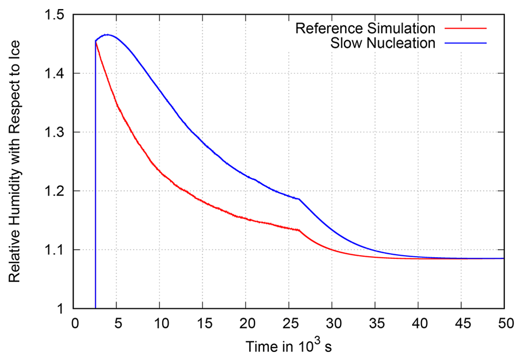
Figure 16Evolution of the in-cloud mean relative humidity in the stochastic box model in a simulation in which α starts at zero at the onset of nucleation in every air parcel and increases over time to s−1 (blue) compared with the reference simulation of the stochastic box model from Fig. 6 with constant s−1 (red). Accounting for the phase of initial crystal growth leads to a short further increase in supersaturation after the onset of nucleation before deposition becomes fast enough to deplete the supersaturation, resulting in a considerable delay in the relaxation process.
Finally, we have also neglected the process of heterogeneous nucleation so far. In order to investigate the influence of ice nucleating particles (INPs) on the evolution of relative humidity in our simulations, we consider the critical number density, Ncr, of INPs derived by Gierens (2003) (Eq. 21 therein), which gives an approximate order of magnitude above which cloud formation is dominated by heterogeneous nucleation. As Haag et al. (2003) suggested that, even in the polluted regions of the Northern Hemisphere, cirrus clouds do not form exclusively via heterogeneous nucleation, we take half of Ncr as our number density of INPs. We introduce it into our stochastic box model by setting a second nucleation threshold at 130 % relative humidity and calculating a corresponding value of α via Eq. (52) for deposition on the resulting heterogeneously nucleated ice particles. In particular, the number density of INPs is 128 m−3 and the corresponding deposition rate is s−1. Consequently, if an air parcel's relative humidity exceeds 130 %, deposition is assumed to occur at this low rate, while α returns to its usual value of s−1 if the parcel's relative humidity exceeds the threshold for homogeneous nucleation. Figure 17 shows the result of this simulation. Intuitively, one might think that introducing another sink for water vapour should reduce the relative humidity. However, apparently the opposite is the case. Heterogeneous nucleation removes moisture from the air parcels with the highest vapour content, while the increase in relative humidity in the dryer parcels remains unchanged. As a result, the threshold for homogeneous nucleation is reached later and the grid-mean relative humidity increases for longer, leading to an overall increased grid-mean relative humidity. Hence, the negligence of heterogeneous nucleation in the new parameterisation does not lead to an overestimation of relative humidity in situations such as the one considered here. Obviously, the picture changes if the number density of INPs exceeds Ncr by far, causing the heterogeneously induced deposition to become fast enough to prevent homogeneous nucleation from occurring. However, according to Haag et al. (2003), such high number densities of INPs should be uncommon.
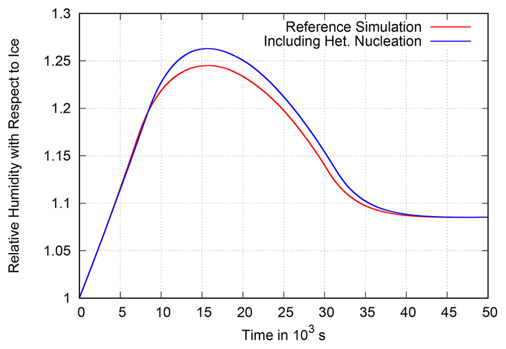
Figure 17Evolution of the grid box mean relative humidity in the stochastic box model in a simulation with a second nucleation threshold at 130 % representing heterogeneous nucleation (blue). For each air parcel, α is set to s−1 once its relative humidity exceeds 130 % and to s−1 once it exceeds the threshold for homogeneous nucleation. The red curve shows the reference simulation of the stochastic box model from Fig. 6 with constant s−1 but starting from 100 % relative humidity. The heterogeneously induced deposition removes vapour from the moistest air parcels, thereby delaying the onset of homogeneous nucleation. This leads to an overall increase in the grid box mean relative humidity.
Further complex influences on the value of α and, therefore, on the distribution of supersaturation within cirrus clouds may arise due to advection and sedimentation processes, which we have not considered thus far in the development of the new concept. A model with saturation adjustment does not have such influences because its α is simply infinite and its distribution of in-cloud supersaturation is a δ function without any sensitivity to other microphysical processes. An investigation of the behaviour of the new parameterisation in a more complete framework that includes advection and sedimentation is outside of the scope of the present paper but is of course the necessary next step in the implementation of the new concept into an actual NWP model.
The mentioned influences on α might be better captured in a two-moment scheme in which information on the ice crystal concentration is available. We expect that a combination of the new concept with explicit in-cloud supersaturation and a two-moment scheme will be fruitful.
In the end, even the best parameterisation will not lead to a temporally and spatially precise prediction of ice supersaturation alone without the aid of relative humidity data for data assimilation, as argued in Sect. 1. The new concept can make the model humidity statistics better match the corresponding statistics from measurements taken over many years in the MOZAIC (Marenco et al., 1998) and IAGOS (Petzold et al., 2015) projects; but this is only a necessary, not a sufficient, condition. More aircraft equipped with hygrometers that work reliably in the upper troposphere are urgently needed.
Tompkins et al. (2007) noticed that many ice-cloud parameterisations suffer from unphysical sub-grid humidity fluxes between the cloudy and the clear-sky portion of a grid box. These fluxes can occur if the specific humidities inside the cloud and in the cloud environment are coupled to the grid mean humidity via a diagnostic assumption. As our parameterisation uses the in-cloud humidity as an additional source of information, there is no need for a diagnostic assumption and unphysical sub-grid humidity fluxes cannot occur, as the in-cloud humidity is processed independently of the grid mean humidity.
Concerning the run time of the new parameterisation, 850 time steps took about 7 ms in the current version, while the parameterisation with saturation adjustment took about 4.5 ms for the same number of steps on the same computer. Furthermore, there will be an increase in the run time of a NWP model due to the additional prognostic variable that is needed in the new parameterisation. Hence, one has to expect additional computational costs when implementing the new parameterisation.
This paper has been written in response to a problem that is probably common to most NWP and climate models, namely the underestimation of both the frequency and degree of ice supersaturation in the upper troposphere. There are many ways that this problem can be tackled and mitigated, ranging from simple corrections to the output humidity field to elaborated cloud microphysics submodels that represent many processes, full size spectra of ice crystals and aerosols, and the complex dynamical background in which the clouds are embedded and in which the microphysics proceeds. Evidently, there is a trade-off between microphysics elaboration and computing effort, and our guideline here is to make better predictions of ice supersaturation in a model that is still cheap and, thus, fast enough that it can serve as a NWP model (which has to obey strict run-time constraints). Therefore, we try to stay with a one-moment scheme, knowing that better but more expensive schemes exist, and we boil down the nucleation and crystal growth physics to a quite simple formulation that is promising with respect to providing a better (albeit not the best) representation of ice supersaturation in NWP models compared with traditional methods that use saturation adjustment. In the sense of “adequacy for purpose” (Gramelsberger et al., 2020; Parker, 2020), we think that this is a good compromise.
In this study, we have introduced the concept of a new parameterisation for the representation of pure ice clouds in NWP models that overcomes the practice of saturation adjustment. This common practice that consists of assuming exactly saturated conditions inside a cloud has been compared to a stochastic box model in which the model grid box is divided into a large number of air parcels. Every air parcel can become cloudy individually if it meets the conditions for nucleation, in which case the humidity inside the parcel is assumed to exponentially decay towards saturation. As this assumption can be considered to be a reasonable approximation to reality, the mean humidity across all air parcels inside this box model serves as a benchmark to estimate the quality of the considered parameterisations.
In this comparison, the parameterisation using saturation adjustment has been shown to underestimate humidity in the presence of a cloud for two reasons:
-
the large supersaturation at the onset of nucleation is converted immediately into ice, which is a process that can take up to hours in weak updraughts in reality;
-
as long as cooling proceeds, it represents a continuous source of new supersaturation such that the cloud remains in a slightly supersaturated state that is not represented in saturation adjustment.
Furthermore, humidity can also be overestimated by saturation adjustment if the temperature inside the cloud is rising. In this case, the ice crystals need time to sublimate such that the air inside the cloud becomes slightly subsaturated, while saturation adjustment again assumes exactly saturated conditions.
This insufficient treatment of in-cloud humidity in current NWP models is one of the factors that hamper a reliable prediction of persistent contrails, which contribute significantly to the overall warming effect of aviation emissions. Our new parameterisation aims to better represent in-cloud humidity by introducing it as a new prognostic variable. Thus, we can explicitly model the decay of the initial large supersaturation right from the onset of nucleation and also represent any super- or subsaturated state in the later life cycle of a cirrus cloud. For this purpose, we derived the humidity distribution in newly generated cloud parts from the stochastic box model.
The new parameterisation has been shown to closely follow the behaviour of the stochastic box model for different updraught scenarios, different rates of exponential humidity decay, different widths of the sub-grid humidity fluctuation distribution and different time step lengths. In particular, it always resulted in an improvement to the saturation adjustment. This improvement is larger if the cloud fraction increases quickly, as this gives more weight to the initially highly supersaturated cloud in the grid box mean humidity – for example, if the sub-grid humidity fluctuations in the clear sky are small. On the other hand, the improvement to the saturation adjustment is small if a large number of ice crystals are generated upon nucleation inside the cloud – for example, in a strong updraught. In this case, the in-cloud humidity relaxes towards saturation quickly and the equilibrium supersaturation that it approaches is also small, as the available surface for the deposition of water vapour is large. However, such conditions are not typical of synoptic-scale cirrus and, hence, a significant improvement compared with a saturation adjustment scheme can be expected.
In reality, the rate of the exponential decay of humidity depends on the number density and the size of the ice crystals inside the cloud and, thus, varies in time. Although this rate has been held constant throughout each of the presented tests of the new parameterisation, first simulations with a variable decay rate have provided promising results. Of course, further tests, especially in a less artificial environment, are needed but we are confident that, despite the additional computational costs, our parameterisation is capable of contributing to a significant improvement in the humidity forecast in the upper troposphere.
Here, we provide details on the derivation of Seq. The defining condition for the equilibrium supersaturation is that a parcel's supersaturation Sp remains unchanged if it equals Seq:
Using the product rule leads to the following:
By moving the second term to the right-hand side of the equation, multiplying it by qs and dividing by qp, we get
This means that, in order for Sp to remain constant, the relative decrease rates of the parcel's specific humidity due to deposition and the saturation specific humidity due to cooling have to equal each other. We now use Eq. (3) to further evolve the expression:
After multiplying this equation by qp and dividing by α and qs, we can identify the equilibrium supersaturation on the left-hand side of the equation and the equilibrium relative humidity, which can be written as Seq+1, on the right-hand side:
Dividing by Seq+1 and taking the reciprocal gives the following:
Here, subtracting 1 and again taking the reciprocal leads to the desired result:
Simulation data are available from https://doi.org/10.5281/zenodo.8413820 (Sperber and Gierens, 2023).
This paper is part of DS's master's thesis. KG conceived of the research, and DS wrote the codes, ran the simulations and produced the figures. Both authors discussed the results and wrote the paper.
The contact author has declared that neither of the authors has any competing interests.
Publisher’s note: Copernicus Publications remains neutral with regard to jurisdictional claims made in the text, published maps, institutional affiliations, or any other geographical representation in this paper. While Copernicus Publications makes every effort to include appropriate place names, the final responsibility lies with the authors.
The authors would like to thank Sabine Brinkop for her helpful comments and grant her a jar of tea in deep gratitude. Two reviewers greatly helped to raise the quality of the paper with their insightful comments, for which we are grateful.
This research has been supported by the Horizon Europe programme (grant no. 101056885).
The article processing charges for this open-access publication were covered by the German Aerospace Center (DLR).
This paper was edited by Toshihiko Takemura and reviewed by Blaž Gasparini and one anonymous referee.
Baumgartner, M. and Spichtinger, P.: Homogeneous nucleation from an asymptotic point of view, Theor. Comp. Fluid Dyn., 33, 83–106, 2019. a
Corti, T. and Peter, T.: A simple model for cloud radiative forcing, Atmos. Chem. Phys., 9, 5751–5758, https://doi.org/10.5194/acp-9-5751-2009, 2009. a
Dekoutsidis, G., Groß, S., Wirth, M., Krämer, M., and Rolf, C.: Characteristics of supersaturation in midlatitude cirrus clouds and their adjacent cloud-free air, Atmos. Chem. Phys., 23, 3103–3117, https://doi.org/10.5194/acp-23-3103-2023, 2023. a
Dietmüller, S., Matthes, S., Dahlmann, K., Yamashita, H., Simorgh, A., Soler, M., Linke, F., Lührs, B., Meuser, M. M., Weder, C., Grewe, V., Yin, F., and Castino, F.: A Python library for computing individual and merged non-CO2 algorithmic climate change functions: CLIMaCCF V1.0, Geosci. Model Dev., 16, 4405–4425, https://doi.org/10.5194/gmd-16-4405-2023, 2023. a
Dowling, D. and Radke, L.: A summary of the physical properties of cirrus clouds, J. Appl. Meteorol., 29, 970–978, 1990. a
Gierens, K.: On the transition between heterogeneous and homogeneous freezing, Atmos. Chem. Phys., 3, 437–446, https://doi.org/10.5194/acp-3-437-2003, 2003. a, b, c
Gierens, K. and Vázquez-Navarro, M.: Statistical analysis of contrail lifetimes from a satellite perspective, Meteorol. Z., 27, 183–193, https://doi.org/10.1127/metz/2018/0888, 2018. a
Gierens, K., Schumann, U., Helten, M., Smit, H., and Marenco, A.: A distribution law for relative humidity in the upper troposphere and lower stratosphere derived from three years of MOZAIC measurements, Ann. Geophys., 17, 1218–1226, 1999. a
Gierens, K., Kohlhepp, R., Dotzek, N., and Smit, H.: Instantaneous fluctuations of temperature and moisture in the upper troposphere and tropopause region. Part 1: Probability densities and their variability, Meteorol. Z., 16, 221–231, 2007. a, b
Gierens, K., Spichtinger, P., and Schumann, U.: Ice supersaturation, in: Atmospheric Physics. Background – Methods – Trends, edited by: Schumann, U., Springer, Heidelberg, Germany, Chap. 9, 135–150, ISBN 978-3-642-30182-7, 2012. a
Gierens, K., Matthes, S., and Rohs, S.: How well can persistent contrails be predicted?, Aerospace, 7, 169, https://doi.org/10.3390/aerospace7120169, 2020. a
Gramelsberger, G., Lenhard, J., and Parker, W.: Philosophical perspectives on Earth system modeling: Truth, adequacy, and understanding, J. Adv. Model. Earth Sy., 12, e2019MS001720, https://doi.org/10.1029/2019MS001720, 2020. a
Haag, W., Kärcher, B., Ström, J., Minikin, A., Lohmann, U., Ovarlez, J., and Stohl, A.: Freezing thresholds and cirrus cloud formation mechanisms inferred from in situ measurements of relative humidity, Atmos. Chem. Phys., 3, 1791–1806, https://doi.org/10.5194/acp-3-1791-2003, 2003. a, b
Heymsfield, A., Krämer, M., Luebke, A., Brown, P., Cziczo, D., Franklin, C., Lawson, P., Lohmann, U., McFarquhar, G., Ulanowski, Z., and Tricht, K. V.: Cirrus Clouds, Meteor. Mon., 58, 1–26, https://doi.org/10.1175/AMSMONOGRAPHS-D-16-0010.1, 2017. a
Kärcher, B. and Lohmann, U.: A parameterization of cirrus cloud formation: Homogeneous freezing of supercooled aerosols, J. Geophys. Res., 107, AAC 4-1–AAC 4-10, https://doi.org/10.1029/2001JD000470, 2002. a, b, c, d, e
Kaufmann, S., Voigt, C., Heller, R., Jurkat-Witschas, T., Krämer, M., Rolf, C., Zöger, M., Giez, A., Buchholz, B., Ebert, V., Thornberry, T., and Schumann, U.: Intercomparison of midlatitude tropospheric and lower-stratospheric water vapor measurements and comparison to ECMWF humidity data, Atmos. Chem. Phys., 18, 16729–16745, https://doi.org/10.5194/acp-18-16729-2018, 2018. a
Khvorostyanov, V. and Sassen, K.: Cirrus cloud simulation using explicit microphysics and radiation. Part I: Model description, J. Atmos. Sci., 55, 1808–1821, 1998a. a, b, c, d, e
Khvorostyanov, V. and Sassen, K.: Cirrus cloud simulation using explicit microphysics and radiation. Part II: Microphysics, vapor and ice mass budgets, and optical and radiative properties, J. Atmos. Sci., 55, 1822–1845, 1998b. a, b
Krämer, M., Schiller, C., Afchine, A., Bauer, R., Gensch, I., Mangold, A., Schlicht, S., Spelten, N., Sitnikov, N., Borrmann, S., de Reus, M., and Spichtinger, P.: Ice supersaturations and cirrus cloud crystal numbers, Atmos. Chem. Phys., 9, 3505–3522, https://doi.org/10.5194/acp-9-3505-2009, 2009. a
Krämer, M., Rolf, C., Luebke, A., Afchine, A., Spelten, N., Costa, A., Meyer, J., Zöger, M., Smith, J., Herman, R. L., Buchholz, B., Ebert, V., Baumgardner, D., Borrmann, S., Klingebiel, M., and Avallone, L.: A microphysics guide to cirrus clouds – Part 1: Cirrus types, Atmos. Chem. Phys., 16, 3463–3483, https://doi.org/10.5194/acp-16-3463-2016, 2016. a
Krämer, M., Rolf, C., Spelten, N., Afchine, A., Fahey, D., Jensen, E., Khaykin, S., Kuhn, T., Lawson, P., Lykov, A., Pan, L. L., Riese, M., Rollins, A., Stroh, F., Thornberry, T., Wolf, V., Woods, S., Spichtinger, P., Quaas, J., and Sourdeval, O.: A microphysics guide to cirrus – Part 2: Climatologies of clouds and humidity from observations, Atmos. Chem. Phys., 20, 12569–12608, https://doi.org/10.5194/acp-20-12569-2020, 2020. a
Lee, D., Fahey, D., Skowron, A., Allen, M., Burkhardt, U., Chen, Q., Doherty, S., Freeman, S., Forster, P., Fuglestvedt, J., Gettelman, A., De León, R., Lim, L., Lund, M., Millar, R., Owen, B., Penner, J., Pitari, G., Prather, M., Sausen, R., and Wilcox, L.: The contribution of global aviation to anthropogenic climate forcing for 2000 to 2018, Atmos. Environ., 244, 117834, https://doi.org/10.1016/j.atmosenv.2020.117834, 2021. a
Marenco, A., Thouret, V., Nedelec, P., Smit, H., Helten, M., Kley, D., Karcher, F., Simon, P., Law, K., Pyle, J., Poschmann, G., Wrede, R. V., Hume, C., and Cook, T.: Measurement of ozone and water vapor by Airbus in-service aircraft: The MOZAIC airborne program, An overview, J. Geophys. Res., 103, 25631–25642, 1998. a, b
McDonald, J.: The saturation adjustment in numerical modelling of fog, J. Atmos. Sci., 20, 476–478, 1963. a
Meerkötter, R., Schumann, U., Doelling, D. R., Minnis, P., Nakajima, T., and Tsushima, Y.: Radiative forcing by contrails, Ann. Geophys., 17, 1080–1094, https://doi.org/10.1007/s00585-999-1080-7, 1999. a
Ovarlez, J., Gayet, J.-F., Gierens, K., Ström, J., Ovarlez, H., Auriol, F., Busen, R., and Schumann, U.: Water vapour measurements inside cirrus clouds in northern and southern hemispheres during INCA, Geophys. Res. Lett., 29, 60-1–60-4, https://doi.org/10.1029/2001GL014440, 2002. a
Parker, W.: Model Evaluation: An Adequacy-for-Purpose View, Philos. Sci., 87, 457–477, https://doi.org/10.1086/708691, 2020. a
Petzold, A., Thouret, V., Gerbig, C., Zahn, A., Brenninkmeijer, C., Gallagher, M., Hermann, M., Pontaud, M., Ziereis, H., Boulanger, D., Marshall, J., Nedelec, P., Smit, H., Friess, U., Flaud, J.-M., Wahner, A., Cammas, J.-P., and Volz-Thomas, A.: Global-scale atmosphere monitoring by in-service aircraft – current achievements and future prospects of the European Research Infrastructure IAGOS, Tellus B, 67, https://doi.org/10.3402/tellusb.v67.28452, 2015. a, b
Petzold, A., Neis, P., Rütimann, M., Rohs, S., Berkes, F., Smit, H. G. J., Krämer, M., Spelten, N., Spichtinger, P., Nédélec, P., and Wahner, A.: Ice-supersaturated air masses in the northern mid-latitudes from regular in situ observations by passenger aircraft: vertical distribution, seasonality and tropospheric fingerprint, Atmos. Chem. Phys., 20, 8157–8179, https://doi.org/10.5194/acp-20-8157-2020, 2020. a
Pruppacher, H. and Klett, J.: Microphysics of clouds and precipitation, Kluwer Academic Publishers, 2nd edn., ISBN 0-7923-4211-9, 1997. a
Schumann, U.: On conditions for contrail formation from aircraft exhausts, Meteorol. Z., 5, 4–23, 1996. a
Schumann, U.: A contrail cirrus prediction model, Geosci. Model Dev., 5, 543–580, https://doi.org/10.5194/gmd-5-543-2012, 2012. a
Schumann, U., Mayer, B., Graf, K., and Mannstein, H.: A parametric radiative forcing model for contrail cirrus, J. Appl. Meteorol. Clim., 51, 1391–1406, 2012. a, b
Spichtinger, P., Gierens, K., Smit, H. G. J., Ovarlez, J., and Gayet, J.-F.: On the distribution of relative humidity in cirrus clouds, Atmos. Chem. Phys., 4, 639–647, https://doi.org/10.5194/acp-4-639-2004, 2004. a
Spichtinger, P., Marschalik, P., and Baumgartner, M.: Impact of formulations of the homogeneous nucleation rate on ice nucleation events in cirrus, Atmos. Chem. Phys., 23, 2035–2060, https://doi.org/10.5194/acp-23-2035-2023, 2023. a
Sperber, D. P. and Gierens, K. M.: Data of “Towards a More Reliable Forecast of Ice Supersaturation: Concept of a One-Moment Ice Cloud Scheme that Avoids Saturation Adjustment”, Zenodo [data set], https://doi.org/10.5281/zenodo.8413820, 2023. a
Stuber, N., Forster, P., Rädel, G., and Shine, K.: The importance of the diurnal and annual cycle of air traffic for contrail radiative forcing, Nature, 441, 864–867, 2006. a
Teoh, R., Schumann, U., Majumdar, A., and Stettler, M.: Mitigating the climate forcing of aircraft contrails by small-scale diversions and technology adoption, Environ. Sci. Technol., 54, 2941–2950, https://doi.org/10.1021/acs.est.9b05608, 2020. a
Teoh, R., Schumann, U., Gryspeerdt, E., Shapiro, M., Molloy, J., Koudis, G., Voigt, C., and Stettler, M. E. J.: Aviation contrail climate effects in the North Atlantic from 2016 to 2021, Atmos. Chem. Phys., 22, 10919–10935, https://doi.org/10.5194/acp-22-10919-2022, 2022. a
Tompkins, A., Gierens, K., and Rädel, G.: Ice supersaturation in the ECMWF Integrated Forecast System, Q. J. Roy. Metor. Soc., 133, 53–63, 2007. a, b
Wegener, A.: Meteorologische Terminbeobachtungen am Danmarks-Havn, in: Meddelelser om Grønland, Vol. XLII: Danmark-Ekspeditionen til Grønlands Nordøstkyst 1906–1908, Kommissionen for ledelsen af de geologiske og geografiske undersøgelser i Grønland, II, 125–356, 1914. a
Wilhelm, L., Gierens, K., and Rohs, S.: Weather variability induced uncertainty of contrail radiative forcing, Aerospace, 8, 332, https://doi.org/10.3390/aerospace8110332, 2021. a, b
Wilson, D. and Ballard, S.: A microphysically based precipitation scheme for the UK meteorological office unified model, Q. J. Roy. Meteor. Soc., 125, 1607–1636, https://doi.org/10.1002/qj.49712555707, 1999. a
Wolf, K., Bellouin, N., and Boucher, O.: Radiative effect by cirrus cloud and contrails – A comprehensive sensitivity study, EGUsphere [preprint], https://doi.org/10.5194/egusphere-2023-155, 2023. a
Yin, F., Grewe, V., Castino, F., Rao, P., Matthes, S., Dahlmann, K., Dietmüller, S., Frömming, C., Yamashita, H., Peter, P., Klingaman, E., Shine, K. P., Lührs, B., and Linke, F.: Predicting the climate impact of aviation for en-route emissions: the algorithmic climate change function submodel ACCF 1.0 of EMAC 2.53, Geosci. Model Dev., 16, 3313–3334, https://doi.org/10.5194/gmd-16-3313-2023, 2023. a
- Abstract
- Introduction
- Stochastic box model and new parameterisation
- Results
- Discussion
- Summary and conclusions
- Appendix A: Derivation of the equilibrium supersaturation
- Data availability
- Author contributions
- Competing interests
- Disclaimer
- Acknowledgements
- Financial support
- Review statement
- References