The role of a low-level jet for stirring the stable atmospheric surface layer in the Arctic

In this study, we analyze the transition of a stable atmospheric boundary layer (ABL) with a low-level jet (LLJ) to a traditional stable ABL with a classic Ekman helix in the late-winter central Arctic. Vertical profiles in the ABL were measured with a hot-wire anemometer on a tethered balloon during a 15 h period in March 2018 in northeast Greenland. The tethered balloon allows high-resolution turbulence observations from the ground to the top of the ABL. The core of the LLJ was observed at about 150 m altitude, and its height and strength were associated with the temperature inversion. Increased turbulence was observed in the vicinity of the LLJ, but most of the turbulence does not reach down to the surface, thus decoupling the LLJ from the surface. Only when the LLJ collapses and the ABL again exhibits a more classical Ekman spiral is a coupling to the surface re-established. The LLJ might enhance both advective and turbulent vertical transport of passive tracers such as aerosol particles or moisture in the often stably stratified Arctic ABL.

1 Introduction

Low-level jets (LLJs) are vertically more or less bounded wind fields with local maximum wind velocities exceeding the geostrophic wind. An LLJ, especially in conjunction with stably stratified boundary layers, is usually found in the upper region of the atmospheric boundary layer (ABL) or even partly just inside or above the inversion. LLJs are often related to inertia oscillations and a decoupling of the flow dynamics from the surface-layer friction (Blackadar, 1957; Smedman et al., 1993). There is a lively debate about the origin of LLJs (Vihma et al., 2011; Jakobson et al., 2013; Tuononen et al., 2015; Guest et al., 2018; Chechin and Lüpkes, 2019), and details of the mechanism behind this are still not completely understood. Polar regions are preferable locations for the occurrence of LLJs (Tuononen et al., 2015; López-García et al., 2022) due to frequently observed (extremely) stably stratified and shallow ABLs, in particular during cloudless (wintertime) conditions with strongly negative thermal-infrared net irradiance. In northeast coastal Greenland, the area of interest for this study, LLJs occur 60 %–70 % of the time, are observed at very low altitudes and are attributed to katabatic flows (Tuononen et al., 2015).

The stably stratified boundary layer, as defined by an increase in potential temperature with height, usually exhibits comparably low turbulence. When neglecting cloud-related effects such as radiative cooling at the cloud top, the only significant source of turbulent kinetic energy (TKE) is the surface roughness. However, due to the strong local wind shear below and above the wind maximum, an LLJ can introduce a significant amount of TKE (Smedman et al., 1993) and modulate the vertical distribution of TKE (Jakobson et al., 2013; Banta et al., 2006). These wind shear zones are usually considered a source of TKE production as long as the damping effect of the inversion does not dominate the TKE production. Boundary-layer flows with a source of turbulence at the top of the inversion generated by vertical wind shear have also been referred to as “upside down” (Mahrt, 1999). The relative importance of turbulence-generating wind shear and damping inversion is quantified by the dimensionless Richardson number (Ri) defined later on. In addition to TKE production, LLJs may play an important role in the advection of momentum, turbulence, and aerosol particles and precursor gases (Stensrud, 1996; Algarra et al., 2019).

Here, we study the ABL evolution in terms of an LLJ, as observed by a set of subsequent vertical wind and temperature profiles measured with a tethered balloon in the framework of the Polar Airborne Measurements and Arctic Regional Climate Model SImulation Project (PAMARCMiP) at Station Nord in northeast Greenland. The central question of this work is how the LLJ might affect the vertical distribution of turbulence and whether increased turbulence is observed at the surface when the LLJ occurs or collapses. This could indicate that properties advected with the LLJ, such as increased aerosol concentration or precursor gases, could also be mixed down to the surface after being advected over a certain distance inside the LLJ.

2 Observations

2.1 PAMARCMiP campaign

The PAMARCMiP field campaign was conducted at the Villum Research Station (VRS) on the military outpost “Station Nord” in the northeast corner of Greenland on the small peninsula of Princess Ingeborg (81^∘36^′ N, 16^∘40^′ W). Balloon observations were made from 10 March to 7 April 2018 about 2 km south of VRS at a small observation hut (“Flygers Hut”) to minimize the station's influence. The site is located on the coastline between the Greenland Ice Sheet to the south and the Arctic Ocean, which is covered with sea ice for most of the year at this location. A glacier is located about 20 km to the south.

The LLJ and ABL structure observations are mainly based on the tethered-balloon system BELUGA (Egerer et al., 2019a). Continuously running meteorological measurements at 9 m altitude at the VRS and three-dimensional wind data from an ultrasonic anemometer (USA-1, manufactured by METEK GmbH, Germany) mounted on a tower at 65 m height support the analysis of the profile measurements.

2.2 The BELUGA setup

BELUGA is a modular system consisting of tethered balloons of various sizes and a variety of sensor packages. During PAMARCMiP, a 9 m³ balloon with a maximum payload of 3 kg was used with multiple sensor packages. The instrument packages were deployed in a rotating sequence aboard BELUGA to ensure adherence to the payload limit; a flight overview table with deployed instruments is provided in Egerer et al. (2019b). In this work, data from two sensor packages are used. (i) A turbulence probe based essentially on a single-component hot-wire anemometer measuring wind speed with a sampling frequency of 500 Hz. A Pitot static tube served as a reference for the hot-wire sensors. Fast temperature measurements were made with a cold-wire sensor. In addition to a calibrated thermometer as a reference for the cold-wire sensor, the data logger provided additional pressure measurements for barometric altitude. (ii) A standard meteorological probe (“StdMeteo”) based on a Graw DFM-09 radiosonde with an additional Pitot static probe provided wind speed and direction using a compass. This package measured wind, temperature and relative humidity at a frequency of 1 Hz and was intended for regular use on all flights. The absolute accuracy of the wind speed measurement with the Pitot static tube is determined by the accuracy of the differential pressure sensor and is additionally inversely proportional to the wind speed itself. For typical wind speeds of 5 m s⁻¹, the absolute accuracy is only in the range of 0.5 m s⁻¹ which is essentially noticeable by a zero offset and can therefore be partially corrected; however, the relative resolution is higher by a factor of 10 for the Pitot static tube and the spectrally determined resolution of the hot-wire anemometer is in the range of 0.2 cm s⁻¹ (Egerer et al., 2019a).

2.3 Measurements and synoptical situation

This study focuses on nine subsequent flights between 10:00 UTC on 29 March and 01:00 UTC on 30 March 2018, during the transition between polar night and day. The period was mainly characterized by the persistent occurrence of an LLJ, followed by a transition to a more classic stable ABL which is characterized by the wind speed increasing mostly logarithmically from the ground with height. The turbulence is generated by the wind shear and is therefore strongest near the ground and decreases continuously with height, depending on the damping effect of the temperature inversion. Synoptic conditions during this period were influenced by high air pressure over central Greenland yielding calm weather conditions at ground level. All flights occurred under cloudless conditions with only thin clouds well above 1000 m. Therefore, possible icing was not an issue.

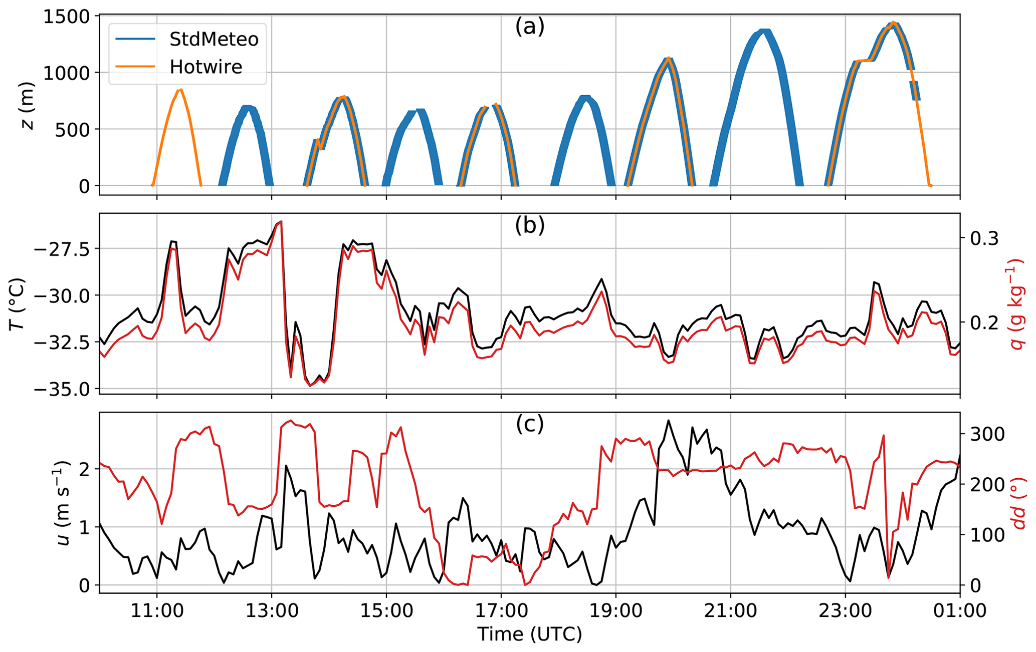
Figure 1 Time series for 29–30 March 2018 of (a) BELUGA flight altitude from the two instrument packages “StdMeteo” and “Hotwire” and (b) VRS near-surface measurements of temperature T and specific humidity q as well as (c) wind velocity u and wind direction dd.

Figure 1 provides an overview of the nine BELUGA flight profiles up to altitudes of 600 to 1400 m in combination with near-surface measurements. The near-surface conditions are quite variable in terms of temperature T and specific humidity q, with T ranging between −35 and −26 ^∘C and q ranging between 0.15 to 0.3 g kg⁻¹. Qualitatively, there is an obvious high correlation between T and q. Wind speeds u were below 2 m s⁻¹ and decreased towards the end of the observation period. The wind direction dd is mainly from the west but turns to being south and then to north from 16:00 UTC and back to west after 19:00 UTC. Between 13:00 and 14:00 UTC, T and q drop abruptly by −8 K and 0.2 g kg⁻¹, respectively, along with a change in wind direction (southeast to north) and reach their previous values about 1 h later.

3 Data analysis methods

In this study, we use the balloon-borne vertical profiles to relate the properties of an LLJ to the vertical structure of stability and turbulence. The literature reveals various definitions of an LLJ, mostly based on a local low-altitude wind velocity maximum greater than around 2 m s⁻¹ (Tuononen et al., 2015; Andreas et al., 2000; Blackadar, 1957). We adopt and slightly modify this definition and define the following criteria for an LLJ: (i) the wind velocity maximum occurs below 250 m altitude, and (ii) the difference between the maximum wind velocity in the LLJ core u_LLJ and the wind minimum u_min above and below (commonly the near-surface wind velocity) exceeds 2.5 m s⁻¹. The LLJ strength is then defined as $\mathrm{\Delta }u=u_{\text{LLJ}}-u_{\text{min}}$ with u_min being the higher value either above or below the jet core. The height of the LLJ core z_LLJ is typically located at the maximum height of the (strong) temperature inversion z_i. We tailor some of the criteria used in the literature to our specific observations and the unique characteristics of this particular LLJ.

The dimensionless gradient Richardson number Ri_g is the ratio of buoyancy to shear:

$$\begin{array}{}\text{(1)}& {\mathit{Ri}}_{\mathrm{g}}={\displaystyle \frac{g}{\stackrel{\mathrm{‾}}{\mathit{\theta }}}}\cdot {\displaystyle \frac{\partial \mathit{\theta }/\partial z}{(\partial u/\partial z{)}^{\mathrm{2}}}},\end{array}$$

with the vertical gradient of the mean flow speed $(\partial u/\partial z{)}^{\mathrm{2}}\approx (\partial u_x/\partial z{)}^{\mathrm{2}}+(\partial u_y/\partial z{)}^{\mathrm{2}}$, the vertical potential temperature gradient $\partial \mathit{\theta }/\partial z$, and the acceleration of gravity g. When stratification dominates over wind shear and a critical Richardson number Ri_c – estimated to be between 0.25 and 1 (Miles, 1961; Abarbanel et al., 1984) – is reached, turbulence decreases. Thus, the contribution of buoyancy and shear to the turbulence profile throughout the ABL can be analyzed by the shear and buoyancy terms of the Ri_g. For estimating Ri_g, u and θ profiles are smoothed with a 10 s rolling mean before calculating the local gradients. The final Ri_g profile is then smoothed again with a rolling mean with a 10 s window. As an approximation for the range between the surface and the core of the LLJ, the bulk Richardson number Ri_b (Mahrt, 1985) is calculated for the height z:

$$\begin{array}{}\text{(2)}& {\text{Ri}}_{\mathrm{b}}\left(z\right)={\displaystyle \frac{g}{\stackrel{\mathrm{‾}}{\mathit{\theta }}}}\cdot {\displaystyle \frac{\mathrm{\Delta }\mathit{\theta }\left(z\right)\cdot z}{\left(\mathrm{\Delta }u\right(z){)}^{\mathrm{2}}}}.\end{array}$$

Here, Δθ(z), or Δu(z), is the difference between θ, or u, at z and close to the surface.

The local turbulence is characterized by means of the local energy dissipation rate ε, which is derived from the second-order structure function of u applying inertial sub-range scaling:

$$\begin{array}{}\text{(3)}& \stackrel{\mathrm{‾}}{{\left(u(t-t^{*})-u\left(t\right)\right)}^{\mathrm{2}}}=C\cdot {\mathit{\epsilon }}^{\mathrm{2}/\mathrm{3}}\cdot {\left(t^{*}\cdot \stackrel{\mathrm{‾}}{u}\right)}^{\mathrm{2}/\mathrm{3}},\end{array}$$

with C=2 and a time lag t^* for the longitudinal wind velocity u (Siebert et al., 2006, Eqs. 10 and 11;). Here, the overline in Eq. (3) denotes time averaging; an averaging interval of 2 s was selected which yields robust estimates (Egerer et al., 2019a). The minimum resolvable ε is estimated to be about 10⁻⁶ m² s⁻³.

To better classify both the integration and averaging times in the determination of parameters as discussed before but also to better interpret the vertical profiles in the next sections, knowledge of the length scales involved is of certain interest. Integral length scales of a turbulent flow, describing the size of the largest energy-containing eddies, can be defined according to

$$\begin{array}{}\text{(4)}& \mathcal{L}=\mathit{\beta }\cdot {\mathit{\sigma }}_u^{\mathrm{3}}/\mathit{\epsilon }.\end{array}$$

(p. 16; Wyngaard, 2010) with a constant β of 𝒪(1). We call the ratio of individual, locally fluctuating $\frac{{\mathit{\sigma }}^{\mathrm{3}}}{\mathit{\epsilon }}$ values “local length scales” ℒ. Here, ε is interpreted as a local parameter derived from 30 s long sub-records to be consistent with ${\mathit{\sigma }}_u^{\mathrm{3}}$ (with σ_u being the standard deviation of u) averaged over 30 s, since σ_u is determined by the largest contributing scales. Earlier studies (Egerer et al., 2019a; Siebert et al., 2006) have shown that the estimation of dissipation rates is insensitive to the choice of the averaging time. Figure 2 shows a scatterplot of ε versus ${\mathit{\sigma }}_u^{\mathrm{3}}$ based on all BELUGA data observed on 29 March 2018. For each measuring point, the corresponding Ri_g value is represented by a color code to better classify the values. The relation of observed ε and ${\mathit{\sigma }}_u^{\mathrm{3}}$ is almost linear as predicted by Eq. (4) but shows some variations. A majority of resulting local length scales (98 % of the data points, assuming β=1) are in the range between 0.1 to 10 m with somewhat larger ℒ in regions of comparably high turbulence (blue–purple colors). A few data points with Ri_g > 1 (yellow color) indicate small length scales below around 1 m. The ratio of the assumed mean wind velocity of $\stackrel{\mathrm{‾}}{u}\approx$ 5 m s⁻¹ to the averaging time of 30 s for estimating σ_u yields an averaging length of 150 m, which is about 10 to 100 times larger than the ℒ estimates. Therefore, we can safely conclude that the averaging period covers enough eddies and the results are statistically robust.

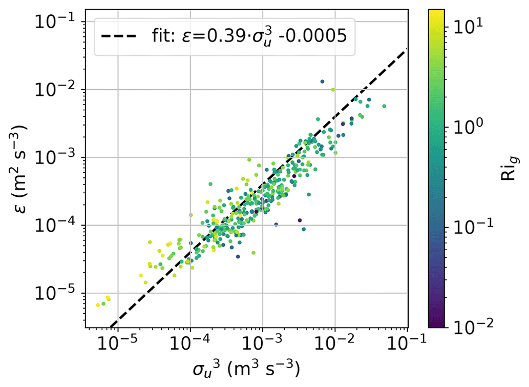
Figure 2 Relation of turbulence parameters for all BELUGA flights on 29 March 2018 with the hot-wire: gradient Richardson number Ri_g, ${\mathit{\sigma }}_u^{\mathrm{3}}$ and local dissipation rate ε. Each dot represents a 30 s time interval of averaged parameters. The dashed line shows a linear regression fitted to the data points.

For the 65 m mast wind data, ε is estimated analogously to the vertical profiles but averaged over 5 min segments and using the vertical wind velocity component. The vertical wind velocity of the 65 m mast sonic anemometer for the flux calculation is tilt-corrected using the double-rotation algorithm described by Wilczak et al. (2001). For the determination of the turbulent fluxes of virtual sensible heat, $H=\mathit{\rho }\cdot c_p\cdot \stackrel{\mathrm{‾}}{{\mathit{\theta }}_v^{\prime }{w}^{\prime }}$, and momentum, ${\mathit{\tau }}_u=\mathit{\rho }\cdot \stackrel{\mathrm{‾}}{u^{\prime }{w}^{\prime }}$, the fluctuations are calculated by applying linear detrending and averaging over 30 min periods at 5 min time steps.

4 Observed vertical structure of the ABL and LLJ

4.1 Evolution of the LLJ and ABL structure

We first analyze the evolution of the mean ABL structure and the LLJ throughout the observation period. Figure 3 provides an overview of the period based on BELUGA profiles (time–height contour plots), VRS observations in terms of meteorological measurements at 9 m and the sonic data at 65 m height. The observation period can be divided into three sub-periods: (i) an LLJ period, (ii) a transition period and (iii) a standard stable ABL. By a “standard stable ABL” we refer to a cloud-free, shallow stable ABL in which terrestrial radiation causes a surface-based temperature inversion, comparable to a nocturnal boundary layer at midlatitudes.

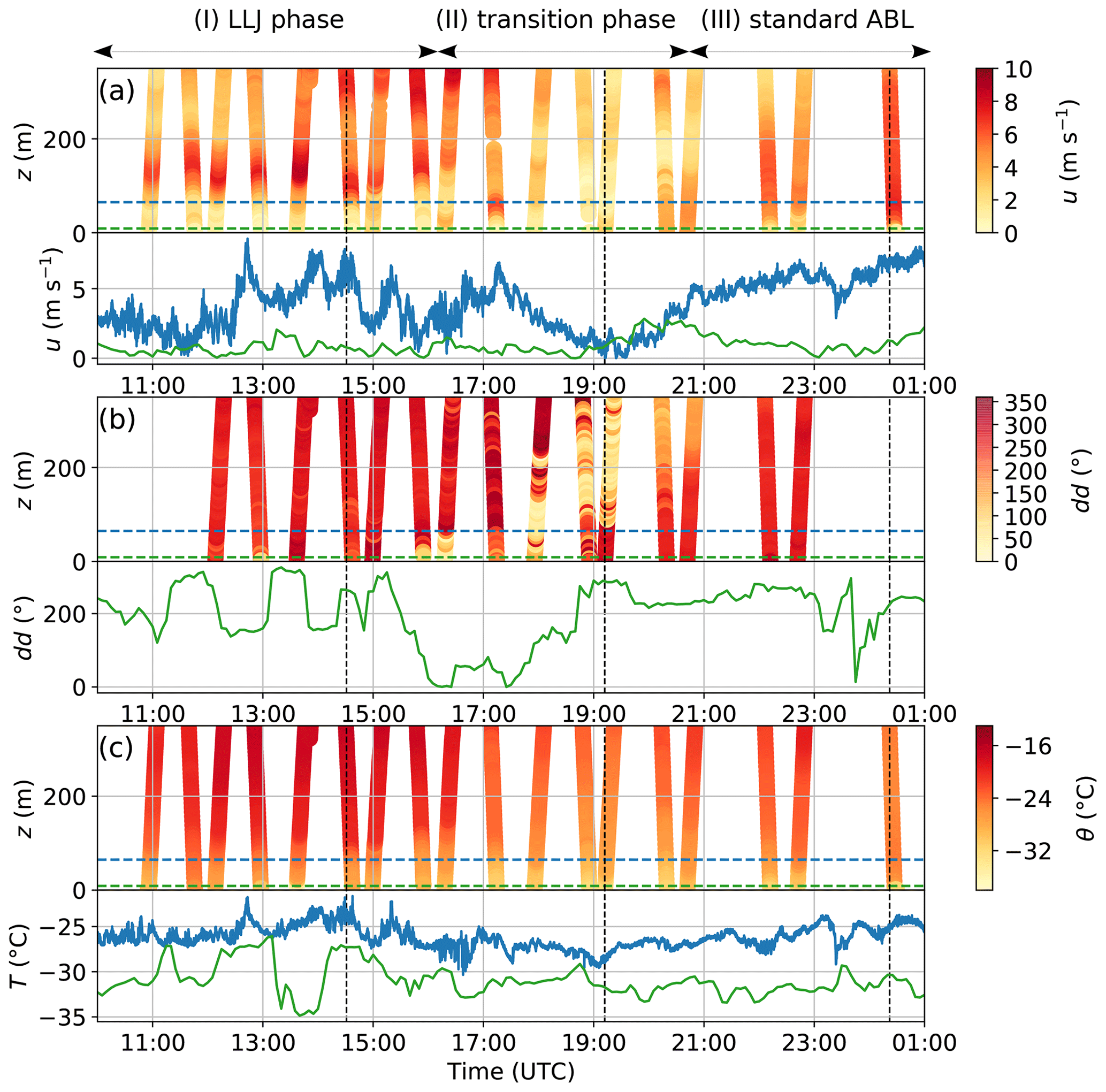
Figure 3 Time–height contour plots and time series observed at 9 m (green) and 65 m (blue) altitude for (a) wind velocity u, (b) wind direction dd, and (c) temperature T or potential temperature θ. The data are from three different sources: (i) the time–height profiles are from BELUGA, (ii) the data shown at 9 m altitude are from VRS and (iii) the data at 65 m altitude are from the mast. The dashed vertical lines represent the time of the example flights in Fig. 4.

In the first period (10:00 to 16:00 UTC), a clear LLJ emerges with a wind velocity maximum of about 10 m s⁻¹ at a height of around 100 to 150 m, while the wind velocity in the near-surface layer remains below 2 m s⁻¹. The wind direction in the lower 400 m is west to northwest with the highest variability at surface level. A very stable surface layer develops with near-surface temperatures around −30 ^∘ C, which increase by 10 K to 100 m height. The sharp surface temperature drop at 13:15 is not obvious at 65 m altitude and qualitatively correlates with a wind rotation to the north.

Between about 16:30 and 21:00 UTC, the wind velocity becomes more constant with height but generally decreases throughout the profile from about 5 m s⁻¹ to less than 2 m s⁻¹ with a highly variable wind direction. The LLJ disappears almost completely, and the strong surface temperature inversion now extends only to the lowermost tens of meters. At 17:00, however, another smaller LLJ occurs with a maximum at a lower altitude compared to the previous LLJs of the first period. The temperature throughout the entire profile decreases by about 5 to 10 K. This period is labeled as a transition between the LLJ period and a standard stable ABL structure.

After 21:00 UTC, the wind velocity increases with a local maximum at around 100 m but is much less pronounced compared to the LLJ structure observed in the first period. The wind direction is almost constant throughout the profile. The temperature profile is similar to the transition phase with a temperature inversion situated at a lower altitude.

For a more detailed analysis of the stratification during the three periods, four selected individual profiles of u, θ and ε are plotted in Fig. 4. A well-developed LLJ is observed at 14:31 UTC. The wind velocity maximum of 9 m s⁻¹ in 100 m coincides with the top of the strong surface-based temperature inversion. Above this inversion, the ABL is almost adiabatically stratified up to 150 m – the region with decreasing wind velocity. This region between 100 and 150 m shows the highest local variability in wind velocity, although the wind shear is lower compared to the height range between 40 and 100 m. This observation is visible in the local energy dissipation, which is highest – apart from the lowermost surface layer – in the upper part of the LLJ. Here, with almost neutral stratification, the wind shear term in Eq. (1) dominates the buoyancy term by 1 order of magnitude. Below the LLJ core at 40 to 100 m, the turbulence generation due to wind shear is reduced (compared to above the LLJ) by the influence of the temperature inversion. A local minimum of ε is located between the surface and the base of the LLJ, where the damping effect of the strong temperature inversion coincides with a height-constant wind velocity. Above 160 m, θ again increases slightly with height and ε drops by 2 orders of magnitude.

The profile observed at 19:12 UTC in the transition phase shows the lowest wind velocity (≈ 1 m s⁻¹) between 50 m and 160 m. The maximum wind velocity is above 3 m s⁻¹ in the near-surface layer, coinciding with a temperature inversion up to 40 m. However, just above this inversion, there is a shallow, 20 m thick layer where the wind shear is strong enough to develop some turbulence indicated by a local maximum of ε up to ${\mathrm{10}}^{-\mathrm{3}}{\mathrm{m}}^{\mathrm{2}}{\mathrm{s}}^{-\mathrm{3}}$. Above and below this maximum, stable stratification in combination with weak wind shear results in reduced turbulence. In the transition phase, one single profile includes an LLJ again, with a slightly different structure than the first period observations (Fig. 4, upper right). Here, the wind velocity increases with height directly above the surface with u_LLJ=7 m s⁻¹ at 60 m height. The lowermost 20 m are neutrally stratified followed by a temperature inversion at z_i=100 m, which coincides with the wind minimum above the LLJ. Here, the ε profile is different from the LLJ cases, with maximum turbulence at the surface, gradually decreasing towards the upper bound of the LLJ, allowing turbulent mixing between the surface and the LLJ core. The upper part of the LLJ is still located inside the temperature inversion, leading to less turbulence in that region than for the LLJ phase. Above the LLJ, the turbulence intensity remains low and slightly increases at higher altitudes, with the wind velocity increasing again.

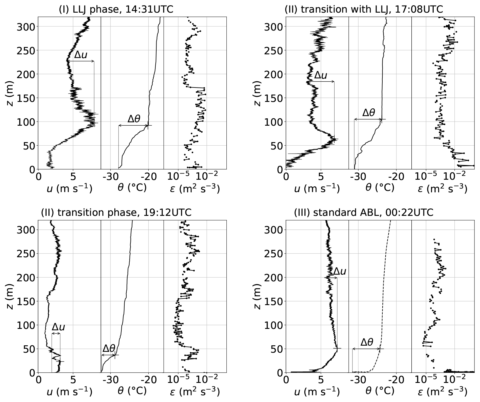
Figure 4 Example vertical profiles for each phase: wind velocity u with the definition of LLJ strength Δu and LLJ height z_LLJ, potential temperature θ with the temperature inversion strength Δθ and inversion height z_i and dissipation rate ε. For the transition phase, one profile with and one profile without LLJ is shown.

In the period with a standard stable ABL structure, the surface layer up to 50 m shows the largest increase in u and θ, thus resulting in generally low values of ε compared to the previous periods. Above 50 m, the ABL is slightly stably stratified with an almost height-constant wind velocity, weakest turbulence at the top of the surface inversion and some variable turbulence at higher altitudes. Throughout the profile, the values for buoyancy and shear increase or decrease to a similar degree, resulting in turbulence predominantly induced by surface roughness.

As a next step, we examine the temporal evolution of LLJ and ABL parameters. Figure 5 shows the time series of LLJ and temperature inversion strength and height, as well as Ri_b between surface and z_i derived from the profiles, combined with continuously measured turbulence parameters at 65 m. Except for a few cases in the transition phase, the LLJ strength correlates with the temperature inversion strength (Pearson correlation coefficient R=0.52). The LLJ height correlates even more clearly with the inversion height (R=0.64). Ri_b is increased in the transition period and around Ri=1 (weak turbulence) for the other two periods. Energy dissipation ε in the LLJ period is 1 order of magnitude higher than in phases II and III and shows much more variability. The turbulent fluxes of heat H and momentum τ_u show increased values and variability and individual events with high flux magnitude in the LLJ period, compared to low fluxes in the transition and standard ABL phase. The LLJ, as observed at 17:04 UTC, coincides with a short period of weak upward-oriented momentum fluxes and downward heat fluxes.

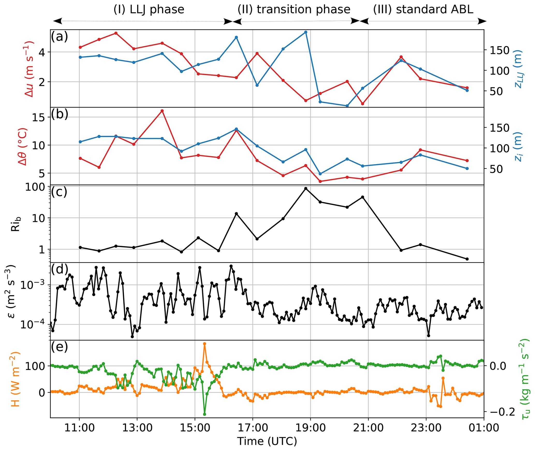
Figure 5 Temporal development of (a) the LLJ parameters strength Δu and height z_LLJ, (b) the temperature inversion strength Δθ and height z_i, (c) bulk Richardson number Ri_b (between surface and z_i), (d) dissipation rate ε at 65 m (5 min averages), and (e) turbulent fluxes H and τ_u at 65 m (calculated every 5 min for a 30 min period).

4.2 Normalized vertical profiles

Each of the three periods introduced in Sect. 4.1 features a distinct vertical structure of thermodynamic and turbulence parameters. For each of the three periods, Fig. 6 shows normalized vertical profiles. Whereas the height is normalized with z_i, u is normalized with u_max (below 300 m), and θ and q are normalized with their values at z_i. The box plots are assigned to height intervals and include median values for each profile within the respective period. The wind velocity profile shows a characteristic shape for the LLJ period and the standard stable ABL period, with low variability within the profiles. The transition phase exhibits much higher variability, and wind velocity increases with height. The θ and q profiles are similar for all phases, with the lowest variability below z_i for the LLJ period. In each period, there is a turbulence maximum in ε close to the surface, which indicates surface-driven turbulence for all cases. In relation to the wind profile, the vertical turbulence profile is different for each period and will be discussed in more detail.

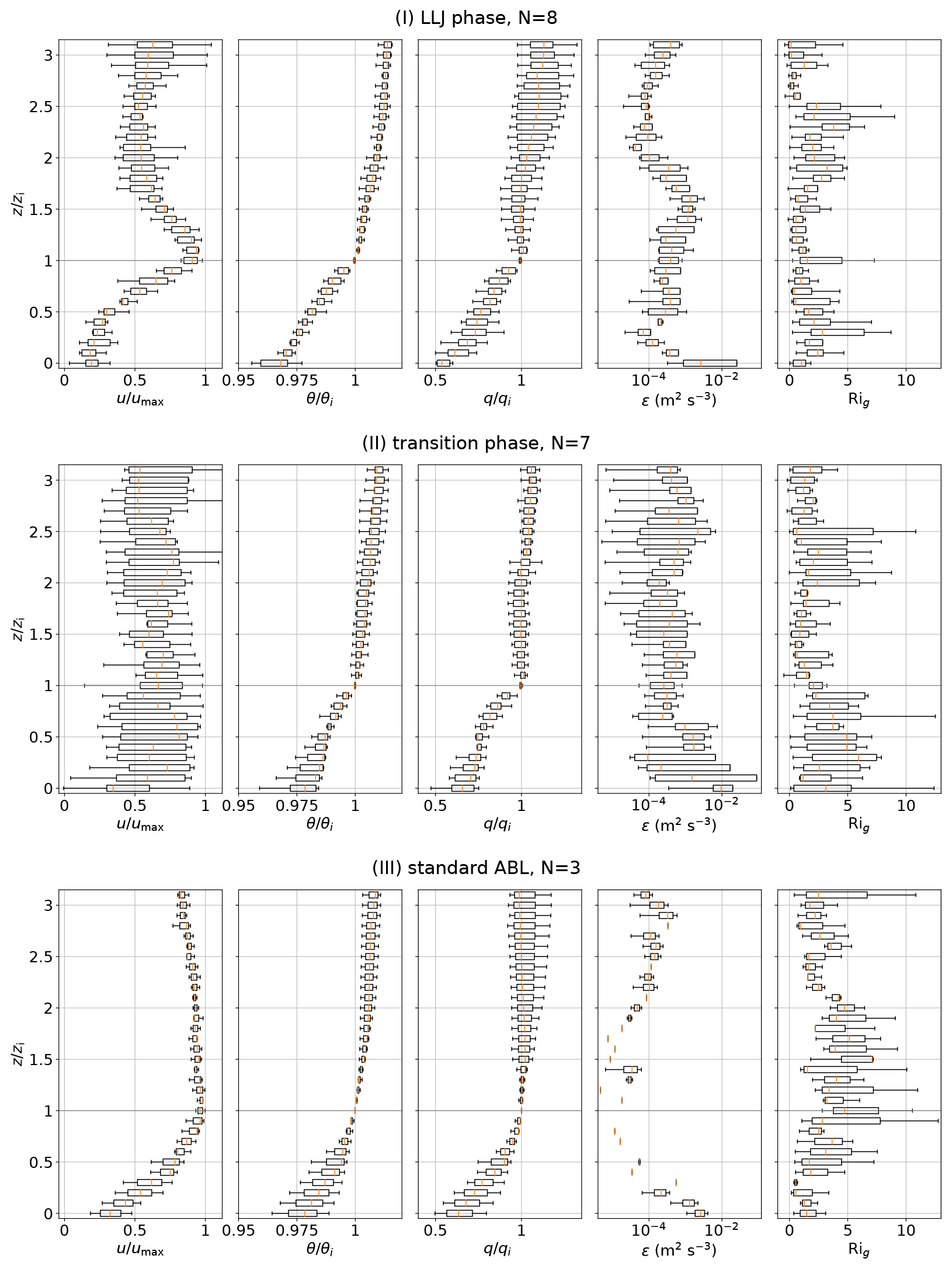
Figure 6 Normalized vertical profiles of u, θ, ε, Ri_g and q for phase I (with LLJ, top), phase II (transition, center) and phase III (profiles without LLJ, bottom). The box plots show variations within the individual N profiles in each phase. The height z is normalized with the temperature inversion base height z_i. The wind velocity is normalized with u_max (u_LLJ or maximum u below 300 m). The quantities θ and q are normalized with their value at z_i. The boxes include the lower and upper quartile values of the data, with the orange line at the median.

In the LLJ period, the average ε structure has a characteristic shape with two local maxima: near the surface and at $z/z_i\approx \mathrm{1.5}$ with reduced values around z_i itself. A local minimum of ε at $z/z_i\approx \mathrm{0.3}$ suggests decoupling of the LLJ from the surface. In the transition period, the average u profile is almost height-constant but shows high internal variability. The ε profile is highly variable with height without any characteristic structure. The only common features are minimum values around z_i and maximum values close to the surface.

The last period is characterized by a gradual increase in the normalized velocity from the surface up to z_i followed by a slight decrease above. Turbulence shows comparably high values only close to the surface with a clear minimum around z_i, where values close to the resolution limit are observed. The low variability within the profiles results partly from only two profiles with turbulence measurements in this phase. The profiles of Ri_g generally match the ε profiles with low Ri_g, correlating with high ε but generally showing a high variability.

These normalized profiles show that the presence of an LLJ enhances turbulent mixing directly above and below the jet maximum compared to a stable ABL without an LLJ. The turbulence increase is more pronounced above the jet core. However, a stably stratified region close to the surface with height-constant wind speeds decouples the LLJ from the surface. The enhanced turbulent mixing by the LLJ might be important for the vertical mixing of advected long-range-transported tracers.

5 Summary and discussion

This study presents the observation of an LLJ based on tethered-balloon measurements in the late-winter central Arctic in March 2018 in northeast Greenland at the Villum Research Station/Station Nord. The measurements span a 15 h period with a transition from a stable ABL with a prominent LLJ to a classically stable nocturnal ABL without an LLJ. The observations include measurements of mean standard meteorological measurements as well as turbulence measurements from the ground to well above the ABL (typically 300 m). The balloon observations were supported by continuous turbulence measurements on a mast at 65 m height – corresponding to the lower part of the LLJ.

During the LLJ phase, observations indicate increased turbulence (increased local dissipation rates) within the LLJ, but the increased turbulence does not reach the surface. Only during the transition phase to a more classical boundary layer structure do these increased turbulence intensities also reach the surface, allowing thorough mixing to occur. These observations lead to the hypothesis that within an LLJ, a passive tracer can be “trapped” and transported over a long distance, without vertical mixing beyond the LLJ boundaries greatly reducing the tracer concentration. Only the dissolution of the LLJ can finally lead to an increased concentration also at the ground.

An accompanying analytical model study (Hellmuth et al., 2023) shows that LLJs may impact aerosol formation and evolution under Arctic conditions. However, the one-dimensional analytical LLJ model revealed difficulties in the reproduction of the observed LLJ wind peak (underestimation of the sharpness of the observed vertical wind velocity), which leads to a misprediction of the shear-induced contribution to the TKE budget. As a consequence, the TKE production at the LLJ level is underestimated. The removal of this shortcoming would require the consideration of momentum advection, baroclinicity and terrain-induced cold-air flow. Nevertheless, within the framework of this conceptual study, we demonstrate that an LLJ can effectively promote the horizontal transport of a passive tracer released close to the ground. This result, in turn, suggests that an LLJ may have a significant impact on both in situ and ex situ aerosol formation and evolution under Arctic conditions. In future research, the simulation of the intrinsically three-dimensional nature of this phenomenon with a more sophisticated model requires further investigation through appropriate observations of the parameters involved, including vertical profiling.