Impacts of maritime shipping on air pollution along the US East Coast

Air pollution is considered a leading threat to human health in the US and worldwide. An important source of air pollution in coastal areas is the globally increasing maritime shipping traffic. In this study, we take a high-resolution modeling approach to investigate the impacts of ship emissions on concentrations of various atmospheric pollutants, under the meteorological conditions and emissions of the year 2018. We utilize the Comprehensive Air Quality Model with extensions (CAMx) to simulate transport, diffusion, and chemical reactions and the Weather Research and Forecasting (WRF) model to provide the meteorological inputs. We focus on four criteria pollutants – fine particulate matter with a diameter smaller than 2.5 µm (PM_2.5), nitrogen dioxide (NO₂), sulfur dioxide (SO₂), and ozone (O₃) – as well as nitrogen oxide (NO), and we calculate their concentrations in the presence and absence of ship emissions along the US East Coast, particularly in the proximity of major ports.

We find that ship emissions increase the PM_2.5 concentrations over the ocean and over a few areas inland. The 98th percentile of the 24 h average PM_2.5 concentrations (the “design value” used by the US Environmental Protection Agency) increased by up to 3.2 µg m⁻³ in some coastal areas. In addition, ships contribute significantly to SO₂ concentrations, up to 95 % over the Atlantic and up to 90 % over land in coastal states, which represents a ∼45 ppb increase in the SO₂ design values in some states. The 98th percentile of the hourly NO₂ concentrations also increased by up to 15 ppb at the major ports and along the shore. In addition, we find that the impact of shipping emissions on O₃ concentrations is not uniform, meaning that ships affect ozone pollution in both positive and negative ways: over the ocean, O₃ concentrations were significantly higher in the presence of ships, whereas O₃ concentrations decreased in the presence of ships in major coastal cities. Our simulation results show that ships emit significant amounts of fresh NO in the atmosphere, which then helps scavenge O₃ in volatile organic compound (VOC)-limited areas, such as major ports. By contrast, over the ocean (NO_x-limited regime), enhanced NO_x concentrations due to ships contribute to the formation of O₃ and therefore enhance O₃ concentrations. Overall, due to the dominant southwesterly wind direction in the region, the impacts of ships on air pollutants mainly remain offshore. However, in coastal states near major ports, the impacts are significantly important.

1 Introduction

Globally, it is estimated that, in 2019, ambient air pollution, particularly particulate matter (PM) and ozone (O₃), was responsible for ∼4.5 million premature deaths worldwide (Fuller et al., 2022). This ranked air pollution as a leading risk factor in the Global Burden of Disease study by the Institute for Health Metrics and Evaluation in 2019 (Murray and Lopez, 1996). Meanwhile, ship traffic is globally increasing and is becoming an important source of air pollution, especially in coastal areas (Corbett and Fischbeck, 1997; Eyring et al., 2010b; Schnurr and Walker, 2019). Sea transport accounts for 80 % of goods transported worldwide (Schnurr and Walker, 2019), while recent studies estimate demand growth of almost 40 % for seaborne trade by 2050 (Serra and Fancello, 2020). Marine vessels are important sources of air pollutants, emitting sulfur oxides (SO_x), nitrogen oxides (NO_x = NO + NO₂), particulate matter (PM), carbon monoxide (CO), volatile organic compounds (VOCs), and carbon dioxide (CO₂) (Corbett et al., 2007; Smith et al., 2015). Low-grade marine fuel oil contains 3500 times more sulfur than road diesel (Wan et al., 2016). Studies reported the fuel consumption of oceangoing ships as being between 200 and 290 Tg (million metric tons) for the year 2000 (Corbett and Köhler, 2003; Endresen et al., 2007). Ships are responsible for about 15 % of all global anthropogenic NO_x emissions and 4 %–9 % of sulfur dioxide (SO₂) emissions. In addition, oceangoing ships are estimated to emit 1.2–1.6 Tg of PM annually (Corbett et al., 2007; Eyring et al., 2010b; Viana et al., 2014).

About 70 % of ship emissions occur within 400 km of the shore (Corbett et al., 1999; Eyring et al., 2005; Endresen et al., 2003). Thus, ships can be a major source of pollution in coastal areas and can impact human health. For instance, ship emissions in East Asia caused 14 500–37 500 premature deaths in 2013, twofold the number reported in 2005 (Liu et al., 2016). Similarly, particulates emitted from ships cause 60 000 cardiopulmonary and lung cancer deaths each year worldwide (Corbett et al., 2007). Studies from different parts of the world, like China, show that shipping emissions increased the annual averaged PM_2.5 concentrations in the eastern coastal regions by up to 5.2 µg m⁻³ and that these enhanced concentrations were carried 900 km inland (Lv et al., 2018). In Europe, although the increase in PM_2.5 concentrations due to ships is found to be small, their relative contribution is large because of the low background PM_2.5 concentrations (Viana et al., 2009; Aksoyoglu et al., 2016).

Fine particulate matter (PM_2.5) is a harmful air pollutant that consists of microscopic particles with a diameter smaller than 2.5 µm. These particles can penetrate human lungs and even the bloodstream and cause serious health problems (US EPA, 2020b). NO_x comprises a group of highly reactive gases; although seven compounds are technically part of the NO_x family (NO; NO₂; nitrous oxide, N₂O; dinitrogen dioxide, N₂O₂; dinitrogen trioxide, N₂O₃; dinitrogen tetroxide, N₂O₄; and dinitrogen pentoxide, N₂O₅), the most abundant are NO and NO₂, but only NO₂ is actually regulated in the US. NO₂ harms humans by irritating the respiratory system, while it harms the environment by creating acid rain (US EPA, 2020a; Lin and McElroy, 2011); it is also a precursor to tropospheric ozone (O₃) formation, which has further negative impacts on human health (EPA, 2020). Similarly, short-term exposure to SO₂ can harm the human respiratory system. These four pollutants – PM_2.5, SO₂, NO₂, and O₃ – are both primary (i.e., they can be directly emitted into the atmosphere) and secondary (i.e., they can also form after chemical reactions in the atmosphere) pollutants. Here, we will focus on these four pollutants which are among the seven “criteria” pollutants that are regulated at the federal level by the US Environmental Protection Agency (EPA) via the National Ambient Air Quality Standards (NAAQS) (US EPA, 2022b).

Due to the complex nature of the atmosphere and its processes, such as chemical reactions, transport, and diffusion, high concentrations of these pollutants are not necessarily found where their emissions are highest. Therefore, although ship emissions are released in marine environments, atmospheric conditions can play an essential role in transporting those pollutants, some of which are precursors for the formation of secondary EPA-regulated pollutants, like O₃.

Ozone pollution is one of the main focuses of this study. The rate of ozone production can be limited by the concentration of either VOCs or NO_x and depends on the relative sources of hydroxyl radical (OH) and NO_x (Finlayson-Pitts and Pitts, 1993). When the rate of OH production is greater than the rate of NO_x production, the rate of ozone production is NO_x-limited. In this situation, ozone concentrations are sensitive to NO_x emissions rather than VOC concentrations. In contrast, when the rate of OH production is less than the rate of NO_x production, ozone production is VOC-limited. In this case, ozone is most effectively reduced by lowering VOC concentrations. NO_x is generally higher where human mobility and transportation are higher (Archer et al., 2020) and, while it is generally NO_x-limited in rural areas and downwind suburban areas, O₃ is often VOC-limited in urban areas with a high population and high traffic emissions (Seinfeld and Pandis, 1998). Motor vehicles are among the major sources of ozone pollution in the region, due to their NO_x and VOC emissions (Niemeier et al., 2006; Yao et al., 2015; Zhang et al., 2014). However, the impact of ocean ship emissions along the US East Coast is lacking in the literature, and we fill this gap in this study. In locations that exceed the EPA ozone standards by only 2–3 ppb, like the small state of Delaware (Moghani et al., 2018), the ship contribution could be of even higher importance.

Here, we explore the impacts of oceangoing ship emissions on the air quality along the US East Coast by utilizing the Comprehensive Air Quality Model with extensions (CAMx) for our simulations. For the first time, we use the most recent high-spatial-resolution (4 km) and high-temporal-resolution (hourly) ship emission data from the EPA's National Emission Inventory (NEI). We also include the ship stack height to account for the vertical layer within which the emissions are emitted into the atmosphere, to be able to account for stability and atmospheric impacts on the pollutants. We investigate the pollution concentrations in a control scenario based on the shipping emissions in the year 2018. Then, we conduct another simulation for a hypothetical condition in which we eliminate the ship emissions altogether while keeping everything else the same. The difference between the two scenarios gives insights into the net contribution of the ships to air pollution.

Seasonal variations in the impact of shipping on various pollutants have been documented in prior studies. For example, Eyring et al. (2010a) noted that during Mediterranean summer conditions, characterized by slow atmospheric transport, strong solar radiation, and limited washout, primary ship emissions accumulate and secondary pollutants form. They reported that secondary sulfate aerosols from shipping were responsible for 54 % of the average sulfate aerosol concentration in the region during the summer. Our findings along the US East Coast align with these results, highlighting the substantial contribution of ships to SO₂ pollution during the summer season. Furthermore, they observed that shipping NO_x emissions could lead to ozone depletion in northern Europe in winter (Eyring et al., 2010a). In a separate study, Eyring et al. (2007) noted significant variations in simulated O₃ levels between January and July, despite a consistent ship emission inventory throughout the year. They found that additional NO_x emissions from shipping led to an O₃ reduction due to titration during winter, while these emissions resulted in relatively modest but positive O₃ concentration changes in regions with sufficient solar radiation in summer. They also showed that the highest ship impacts on O₃ due to ship emissions were found in July and April, whereas the impacts were smaller in October and January (Eyring et al., 2007). In this study, however, we base our analysis on the summer (1 June–31 August) when the highest-O₃ episodes occur.

2 Methods

2.1 Setup of the WRF-CAMx modeling system

We take a modeling approach to explore the pollution concentration across the study domain. The models used in this study are the Weather Research and Forecasting (WRF) model, version 4.3, and the Comprehensive Air quality Model with extensions (CAMx), version 7.1, with the Carbon Bond version 6 revision 5 (CB6r5) chemical mechanism. WRF is developed at the National Center for Atmospheric Research (NCAR) (Skamarock et al., 2019) and is one of the most widely used numerical weather prediction models. CAMx is a modular, Eulerian, 3D photochemical air quality model (Ramboll Environment and Health, 2020) that simulates the emission, production, advection, diffusion, chemical transformation, and removal of atmospheric pollutants at regional scales, and it is among the few that are recommended by the EPA for regulatory purposes (US EPA, 2022a). We use the WRF-CAMx modeling system to conduct simulations of two separate scenarios, based on the exact same setup and inputs: the first scenario includes the ship emissions (WithShips), whereas we remove the ship emissions altogether in the second hypothetical scenario (NoShips). The difference in pollution levels between the two cases provides the net contribution of ship emissions to regional air quality.

CAMx requires input data to characterize meteorology and chemistry, initial and boundary conditions for all of the modeling domains, and other environmental conditions such as the photolysis rates. Meteorology is an essential factor in the formation of many secondary pollutants, both directly and indirectly. Atmospheric stability plays a significant role in determining pollutant faith (Arya, 1999). In CAMx, the plume rise calculations for point sources including the commercial marine vessel (CMV) emissions depend on meteorological conditions and atmospheric stability to determine which vertical layer the emissions are emitted in. In the summertime, various atmospheric stabilities have been found to be dominant over the Atlantic Ocean depending on the location (Golbazi et al., 2022; Golbazi and Archer, 2019; Archer et al., 2016). We use the WRF model to provide meteorological inputs to CAMx. The publicly available WRF-CAMx data-processing program (Ramboll Environment and Health, 2020) is used to generate CAMx meteorological input files from WRF output files. Details on the WRF model setup are provided in Table 1. Our period of study is the summer of 2018, selected to reflect the most recent emission inventory available (discussed next in Sect. 2.2). Photolysis rate inputs to CAMx were calculated using the Tropospheric Ultraviolet and Visible (TUV) radiative transfer and photolysis model (https://www2.acom.ucar.edu/modeling/tropospheric-ultraviolet-and-visible-tuv-radiation-model, last access: 12 January 2023).

Table 1 Details of the WRF-CAMx model setup.

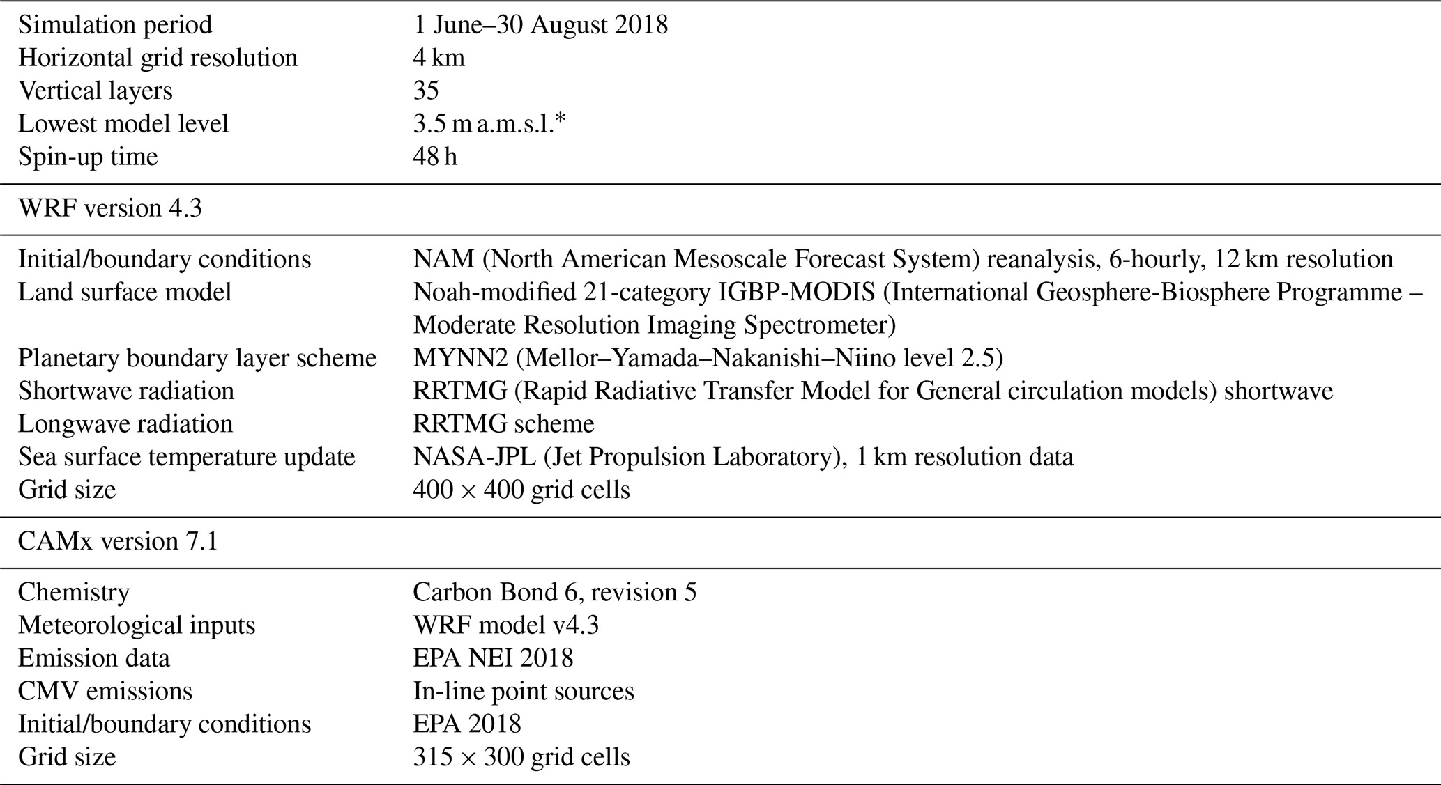
^*“m a.m.s.l.” denotes meters above mean sea level.

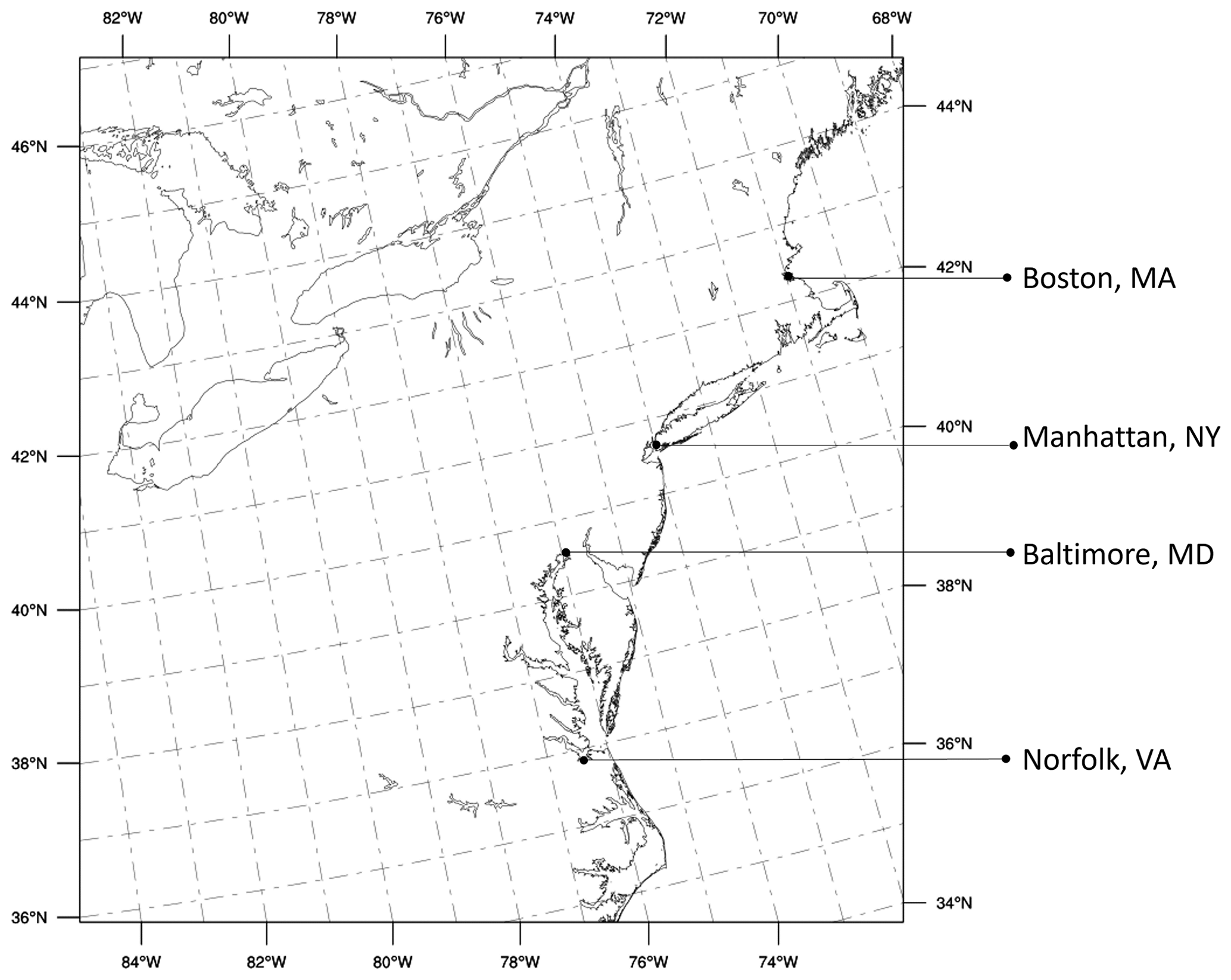
Figure 1 The 315×300 grid cell study domain with a 4 km horizontal grid resolution.

The domain of this study covers the US East Coast (Fig. 1) and includes major cities and highly populated regions. Furthermore, it contains several major ports, which are found to experience high shipping traffic. The meteorological files have 400×400 horizontal grid points covering the entire CAMx domain, which consists of 315×300 grid points, the same as the emission files. We impose 35 vertical levels that are closely spaced near the surface and then gradually expand. The top hydrostatic pressure is 20 hPa, and the lowest model level is at approximately 3.5 m a.m.s.l. (meters above mean sea level). Details about the model configuration are discussed in Table 1. Both the WRF and CAMx models have a 4 km horizontal resolution, the same as the emission inventory, in order to avoid spatial interpolation of gridded emission data. To minimize the impacts of the initial conditions on modeling results, we consider at least 48 h of spin-up time for both models. Furthermore, as the areas of interest are far from the boundaries, the effects of boundary conditions on modeling results are expected to be minimal.

2.2 Emission data

For emission inputs, we use the most recent emission inventory (Long Island Sound Tropospheric Ozone Study, LISTOS, data) developed by the EPA, which includes the period from 1 May to 1 October 2018 (US EPA, 2017) at a 4 km horizontal grid resolution and an hourly temporal resolution. The emissions are distributed on a 315×300 grid, which covers the entire US East Coast (Fig. 1), with 35 layers vertically. Emissions are treated in two basic ways within CAMx: gridded 2D emissions that are released into each grid cell of the modeling domain near the surface (i.e., “area sources”, such as traffic or residential heating) and stack-specific “point sources”, where each stack is assigned unique coordinates and parameters (i.e., smokestacks or ship chimneys). For in-line point source emissions, CAMx computes the plume rise using stack parameters and the hourly emissions for each emission sector.

The 2018 NEI data are based on the year 2017 activity. They contain merged gridded 2D surface emissions, meaning that they are provided as one set of surface emissions that include all of the existing 2D emission sectors, such as all anthropogenic emissions, aircraft emissions, on-road and non-road emissions, railroad emissions, and agricultural emissions. They also include biogenic emissions. The 2018 inventory lacks the wildfire emissions for this time and domain. However, our investigation through the wildfire history shows that 2018 was a year with a low number of wildfires, especially along the East Coast (https://www.nifc.gov/fire-information/statistics/wildfires, last access: 12 January 2023); therefore we do not believe that wildfire emissions significantly impact our findings. Nonetheless, in future studies, including wildfire emissions (based upon availability) is recommended. In contrast to the 2D gridded emissions, the elevated point sources in this inventory are provided for each respective sector.

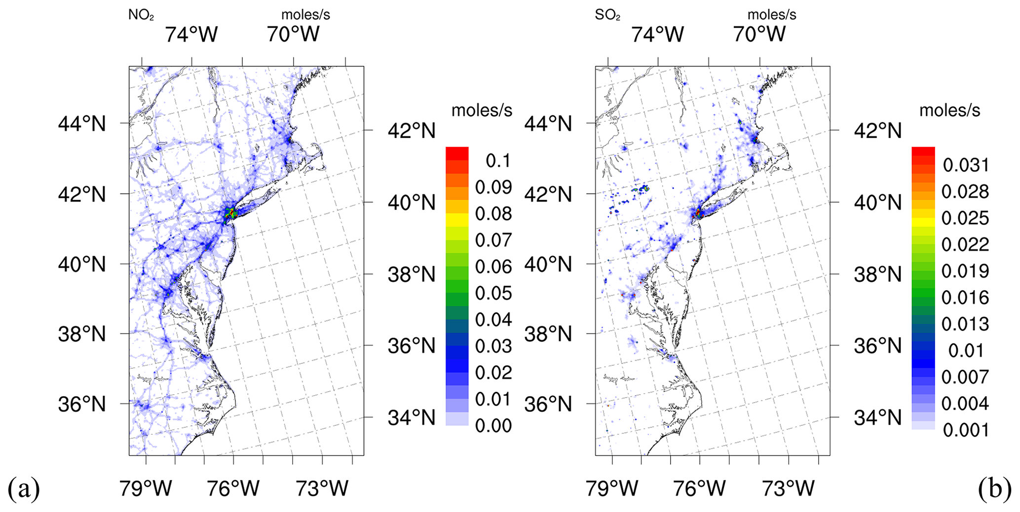
Figure 2 Gridded 2D emission distribution across the domain (averaged over time) in moles per second for (a) NO₂ and (b) SO₂. The gridded emissions include all of the 2D anthropogenic and biogenic emissions and exclude the elevated point sources.

For the ship emissions, we use the emission data for the commercial marine vessel (CMV) sector, which includes category-1, category-2 (small engine), and category-3 (large engine) ships. These emissions are calculated based on the ship's fuel consumption, ship engine type, ship activity, and emission factors specific to those characteristics. The EPA's CMV estimates are computed using detailed satellite-based automatic identification system (AIS) activity data from the United States Coast Guard (US Environmental Protection Agency, 2021, 2020). Other point sources present in this inventory include electric generation units, point oil and gas sources, and any other point sources. CAMx computes the time-varying buoyant plume rise using stack parameters and the hourly emissions for each emissions sector, including CMV. Unlike previous EPA datasets, the CMV emissions in 2018 are at a 1 h temporal resolution, which is very important and makes this study the first to utilize hourly emissions for ships. The initial and boundary conditions for this study are also provided by the EPA and are products of the GEOS-Chem model.

The spatial distribution of the 2D gridded merged anthropogenic emissions are illustrated in Fig. 2. It is important to note that O₃ is a secondary pollutant, meaning it is not directly emitted into the atmosphere. Conversely, PM_2.5 is either a primary or secondary pollutant. Hence, we have specifically generated gridded emission maps for NO₂ and SO₂, only. The distribution of NO₂ emissions closely mirrors the pattern of major highways and roads, as transportation stands out as one of the most significant emission sources for nitrogen oxides (NO_x). The objective of this figure is to explain the spatial distribution of gridded anthropogenic emissions, shedding light on how concentrations change (Figs. 6a, 7a) in relation to their emission sources.

3 CAMx model performance analysis

The primary goal of this study is to explore changes in pollution levels between the two examined case studies, one involving the presence of ships and the other without the presence of ships. Despite the instances where CAMx may either under- or overestimate pollutant concentrations, it is noteworthy that the model bias remains the same in both scenarios. Consequently, we hold the view that these outcomes are unlikely to have a significant influence on our analysis. Nevertheless, we have thoroughly evaluated the model's performance to maintain transparency in our findings. It is important to acknowledge that uncertainties in air quality modeling can arise from various sources, such as uncertainties in emission inventories (Foley et al., 2015), the accuracy of meteorological inputs (Kumar et al., 2019; Ryu et al., 2018; Zhang et al., 2007), numerical noise inherent in the model (Ancell et al., 2018; Golbazi et al., 2022), and numerical approximations.

For our evaluation process of these four pollutants, we rely on measurement data sourced from the EPA's AirNow program, which are publicly accessible (https://aqs.epa.gov/aqsweb/documents/data_api.html, last access: 12 January 2023). Within the geographical scope of our study, we have access to data from a network of monitoring stations. Specifically, there are a total of 196 stations providing data for O₃, while 87, 73, and 118 stations supply data for SO₂, NO₂, and PM_2.5, respectively. This extensive dataset forms the basis of our assessment, enabling us to comprehensively evaluate the CAMx model's performance with respect to replicating real-world air quality conditions for these pollutants. It is worth mentioning that evaluating PM_2.5 presents challenges due to the nature of EPA-reported PM_2.5 measurements in the AirNow database. These values are directly obtained through instrumental measurements, classifying any particle smaller than 2.5 µg as a PM_2.5 species. This method does not provide a clear means of distinguishing between the various particles detected by these instruments. In contrast, the PM_2.5 species in our study are defined based on CAMx model documentation (Ramboll Environment and Health, 2020). This divergence in approach makes a comprehensive PM_2.5 evaluation challenging, and pursuing alternative assessment methods falls beyond the scope of our current study.

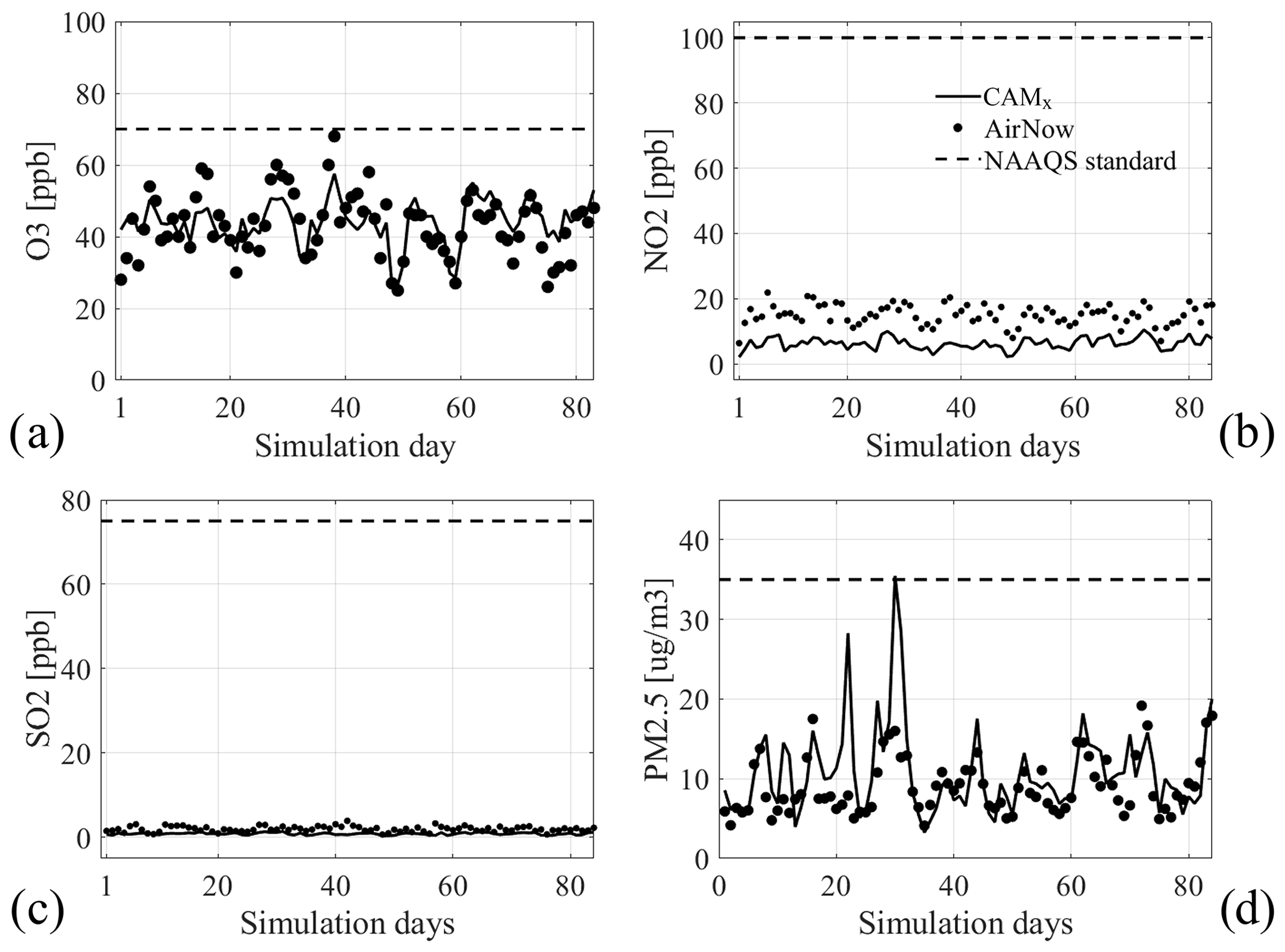
Figure 3 Time series of the model versus observations: CAMx model performance evaluated against the AirNow measurements. The time series are averages calculated across all stations for each day for (a) O₃ (ppb), (b) NO₂ (ppb), (c) SO₂ (ppb), and (d) PM_2.5 (µg m⁻³).

Figure 3 illustrates the time series of the AirNow measurements (black circles) across the simulation days as well as the co-located CAMx outputs (solid black line) for the pollutant of interest. The co-located data are such that they are extracted at the same hour as observations and at the mass point of the grid cell that contains that specific station. Figure 4, on the other hand, illustrates the mean bias error (MBE) calculated at every station and depicts a spatial distribution of the model MBE for each pollutant using the co-located data. CAMx demonstrates a tendency to slightly under- or overestimate O₃ concentrations closer to the coast or away from the coast, respectively (Fig. 4a). Our focus is mainly on locations closer to the coast, as that is where we detect the highest impact of shipping emissions. For O₃, a calculated MBE of −1.12 ppb indicates a systematic underestimation of around 2.5 % across all monitoring stations within the designated domain. Overall, the model effectively captures the O₃ trend and demonstrates a satisfactory level of agreement with observational data, as illustrated in Fig. 3a. In addition, CAMx showcases a strong alignment with observational data in terms of SO₂ simulations with minimal deviation from the observations.

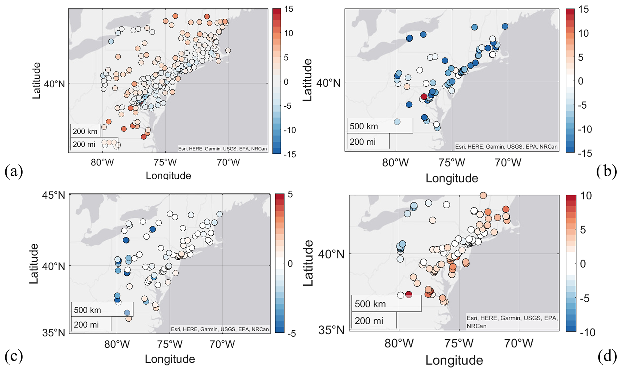
Figure 4 CAMx model performance against the AirNow observations: the MBE calculated at each station for (a) O₃ (ppb), (b) NO₂ (ppb), (c) SO₂ (ppb), and (d) PM_2.5 (µg m⁻³). Blue shades show a systematic underestimation, whereas red shades illustrate a systematic overestimation by the model.

For PM_2.5, the model typically underestimates high-PM_2.5 episodes, as has commonly been observed in prior studies (Delle Monache et al., 2020; Golbazi et al., 2023). Nonetheless, for the remainder of the time, it demonstrates a strong alignment with observed data, as shown in Fig. 3d. Figure 4d reveals that the model bias for PM_2.5 consistently remains below 5 µg m⁻³ for the majority of coastal stations, with only a few exceptions.

Shifting focus to NO₂, the model systematically underestimates NO₂ concentrations (Figs. 3b, 4b). This observation aligns with findings reported in existing literature (Ma et al., 2006). The notable underestimation of NO₂ levels within the model can be attributed to the fact that the monitoring stations are typically situated in close proximity to major roadways characterized by a heavy traffic flow, resulting in elevated NO₂ emissions. Conversely, NO₂ concentrations at locations farther away from these monitoring stations tend to be significantly lower than those recorded by the sensors near high-traffic roads (Fig. 2a). On the other hand, in the CAMx model, data are extracted from the nearest central mass point within a grid cell containing the AirNow station's location, providing an averaged representation of NO₂ levels within that specific grid cell. Consequently, the inherent positive bias in observations contributes to the model's tendency to underestimate this pollutant.

4 Results and discussion

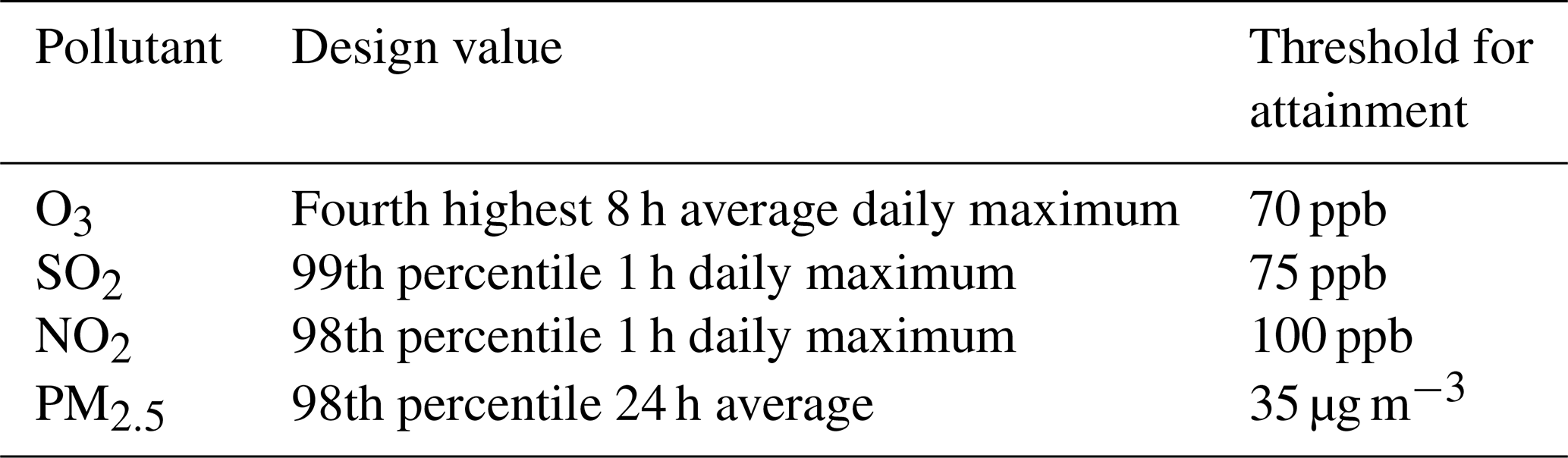
We study the impacts of ship emissions on the concentrations of four criteria pollutants: PM_2.5, SO₂, NO₂, and O₃. We calculate the time-averaged concentrations over different time periods depending on the pollutant (to match the EPA national standards) as follows: 1 h for SO₂ and NO₂, 8 h for O₃, and 24 h for PM_2.5. We analyze every pollutant from two perspectives: (1) from a regulatory perspective, thus calculating the statistics that are as close as possible to the EPA design value for each pollutant (Table 2), and (2) from a worst-case perspective, thus calculating the maximum contribution of ships to each pollutant over the entire 3-month study period.

Table 2 Design values for criteria pollutants (US EPA, 2022b). For attainment purposes, the design values should be calculated by taking the average of the various percentiles over the past 3 years; as only 1 year was simulated in this study, the 3-year average could not be calculated and, therefore, only the actual percentiles were used.

To calculate the maximum contribution, we first find the differences between the two cases (WithShips minus NoShips) at every grid cell, averaged over the relevant time interval, which depends on the pollutant (Table 2); then, we find the maximum difference through the 3 months at every grid cell as follows:

$$\begin{array}{}\text{(1)}& \max \left(\mathrm{\Delta }{P}_{i,j}\right)={\max }_{t\in \left[\mathrm{1}\mathrm{\dots }n\right]}\left(P_{i,j}^{\mathrm{WithShips}}\left(t\right)-P_{i,j}^{\mathrm{NoShips}}\left(t\right)\right),\end{array}$$

where n is the number of data on the 1, 8, or 24 h averaged pollutant (P) concentration values (the exact time-averaging window depends on the pollutant; see Table 2) over the 3-month period of study; P^WithShips and P^NoShips are pollutant P concentrations with and without the ships, respectively; and i and j correspond to the model grid cell indices.

Although the maximum contribution from Eq. (1) is not valuable in terms of reaching or maintaining the EPA attainment for states, it is essential to understand the importance of maritime shipping on air quality, both physically and statistically. A summary of the design values defined here for each pollutant to represent the EPA standards and the threshold for attainment are presented in Table 2. The defined design values follow the same criteria as defined by the EPA (US EPA, 2022b) but only for the time period of this study. For the remainder of the article, we will assume that the design values defined in Table 2 serve the purpose of analyzing the pollution from a regulatory perspective and are the same as the EPA standards for those pollutants for the time period of this study.

We find that the concentration of carbon monoxide (CO) remains unchanged in the presence of ships (not shown), suggesting that the CMV sector has minimal impact on the CO concentrations in the region. As such, we do not discuss the CO results further.

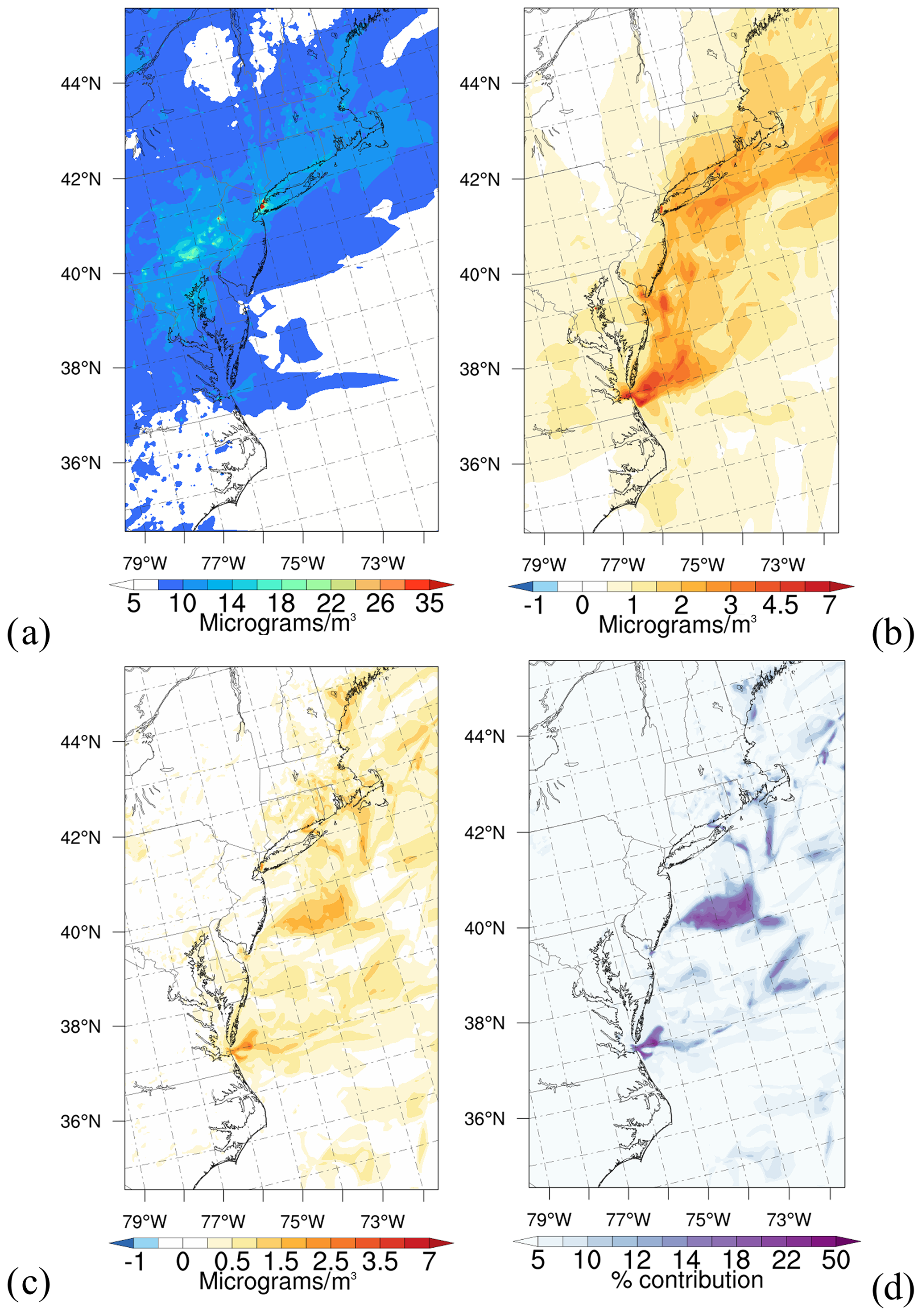
Figure 5 PM_2.5 concentration results: (a) 98th percentile of the 24 h average PM_2.5 concentrations with ships (WithShips); (b) maximum contribution of the ships during the 3-month period (Eq. 1); (c) difference between the two scenarios (WithShips minus NoShips) from a regulatory perspective, meaning the changes in the 98th percentile PM_2.5 concentrations; and (d) percent contribution of the ships to 98th percentile of the 24 h average PM_2.5 concentrations.

4.1 Fine particulate matter (PM_2.5)

The PM_2.5 species used in this study are those included in the CAMx model output (Ramboll Environment and Health, 2020). The EPA requires that the 3-year average of the 98th percentile of the daily mean PM_2.5 concentrations should not exceed 35 µg m⁻³. Here, we calculated the 98th percentile of the 24 h averaged PM_2.5 concentrations at every grid cell during the simulation period in both scenarios, WithShips and NoShips.

We find that PM_2.5 levels stayed below 35 µg m⁻³ across most of the domain and that only two locations, i.e., Manhattan, New York (NY), and Easton, Pennsylvania (PA) (Fig. 5a), crossed the 35 µg m⁻³ maximum allowed concentration and, therefore, were in non-attainment based on the design value defined in Table 2 in this study. From a policy perspective, the CMV sector increases PM_2.5 levels up to 3.2 µg m⁻³ in Manhattan, NY, and up to 2 µg m⁻³ elsewhere (Fig. 5c). This is while the contribution (in %) to PM_2.5 concentrations remains below 27 % across the domain (Fig. 5d). In a worst-case scenario, however, the maximum contribution of ships to PM_2.5 concentrations within the 3 months is significantly high across the domain, but, due to the dominant southwesterly wind direction in the region (Golbazi et al., 2022), it mostly remains over the Atlantic Ocean (Fig. 5b). The maximum impact on PM_2.5 during the 3 months reaches as high as 8 µg m⁻³. Across the domain, the highest impacts are found offshore of MD and VA and in the Chesapeake Bay, Delaware (DE). Over land, the highest impacts are in Manhattan, NY, Connecticut (CT), and coastal Massachusetts (MA).

4.2 Sulfur dioxide (SO₂)

The SO₂ design value is defined as the 99th percentile daily maximum SO₂ concentrations in the simulation period, which should not exceed 75 ppb (Table 2). Here, we calculated the 99th percentile of daily maximum SO₂ concentrations at every grid cell over the simulation period in the two scenarios, i.e., WithShips and NoShips. Then, we subtracted these two cases from one other (WithShips minus NoShips) to obtain the net effect of the maritime shipping sector.

Our results show that ships have a significantly high impact on SO₂ concentrations, up to 95 % and 90 % over the Atlantic Ocean and inland areas, respectively (Fig. 6d). This suggests that the CMV sector is one of the highest contributors to SO₂ levels in the region. The increase in the SO₂ design value for ships remains mainly offshore and around the major shipping routes (Fig. 6c). However, it reaches interior inland regions at major ports and in some parts of the coastal states. Over the simulation period, the contribution of the ships to the 99th percentile daily SO₂ maxima is up to ∼45 ppb, with the highest impact in Baltimore; Maryland (MD); Norfolk, Virginia (VA); and parts of New Jersey and Long Island (Fig. 6c). We note, however, that the SO₂ design value in the region remained below 75 ppb in all states (Fig. 6a). It is worth mentioning that the locations with the highest SO₂ concentrations are the ones highly impacted by ships.

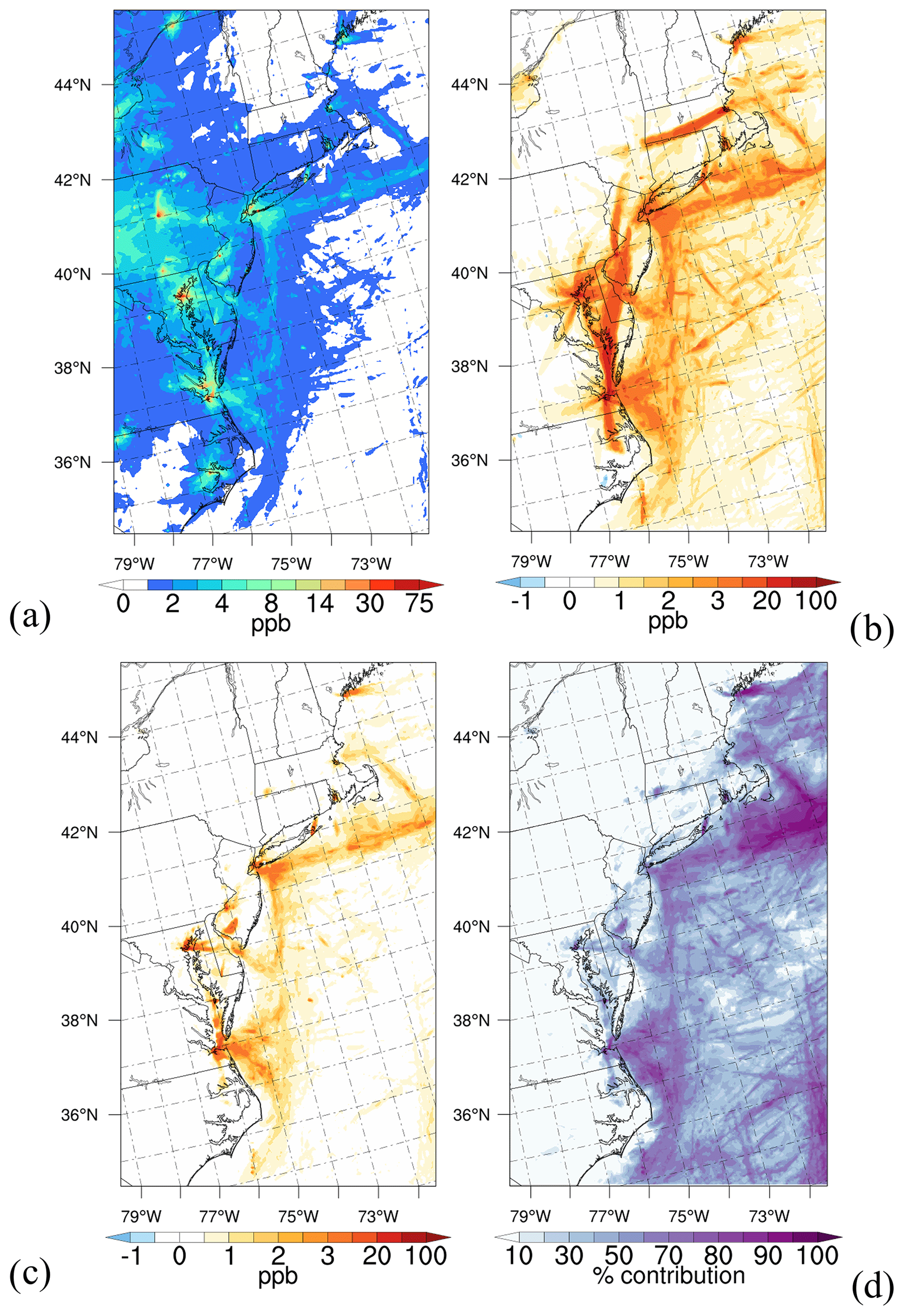
Figure 6 SO₂ concentration results: (a) 99th percentile of daily 1 h maximum SO₂ concentrations with ships (WithShips); (b) maximum contribution of the ships during the simulation period (Eq. 1); (c) differences between the 99th percentile daily maximum between the two scenarios (WithShips minus NoShips); and (d) contribution (in %) of the ships to the 99th percentile of the daily SO₂ maximum.

In addition, we calculated the 3-month maximum contributions of ships to SO₂ concentrations, which indicates the worst-case scenario at every grid cell (Fig. 6b). Although the increase in the SO₂ design value was mainly offshore, the maximum contribution of ships to SO₂ showed a different pattern, with a maximum increase of up to ∼185 ppb at a few grid cells around Norfolk, VA. We note that an occasional and short-term spike of high SO₂ concentrations, as we report here for Norfolk, is not necessarily associated with a strong health impact.

4.3 Nitrogen dioxide (NO₂)

NO₂ is a precursor to tropospheric ozone (O₃) formation, which has further negative impacts on human health (EPA, 2020). NO₂ is generally directly emitted into the atmosphere from emission sources, including ships. We find that ships cause a significant increase in the 98th percentile of daily maximum NO₂ concentrations, up to 34 ppb, although only at a few locations along the coast and in coastal states with major ports (Fig. 7c), suggesting that, except for states with large ports, ships do not significantly impact the state compliance with the EPA standards. However, in NC, VA, DE, NY, and CT, the shipping impacts reach beyond 15 ppb from a regulatory standpoint. Among these states, while NC remains in attainment with regulations (below 100 ppb), it experiences up to an 80 % contribution from ships to its NO₂ concentrations. On the other hand, NY is the only state in the study domain that exceeds the 100 ppb standard for NO₂ concentrations, and the shipping contribution to its non-attainment is 20 %–25 %.

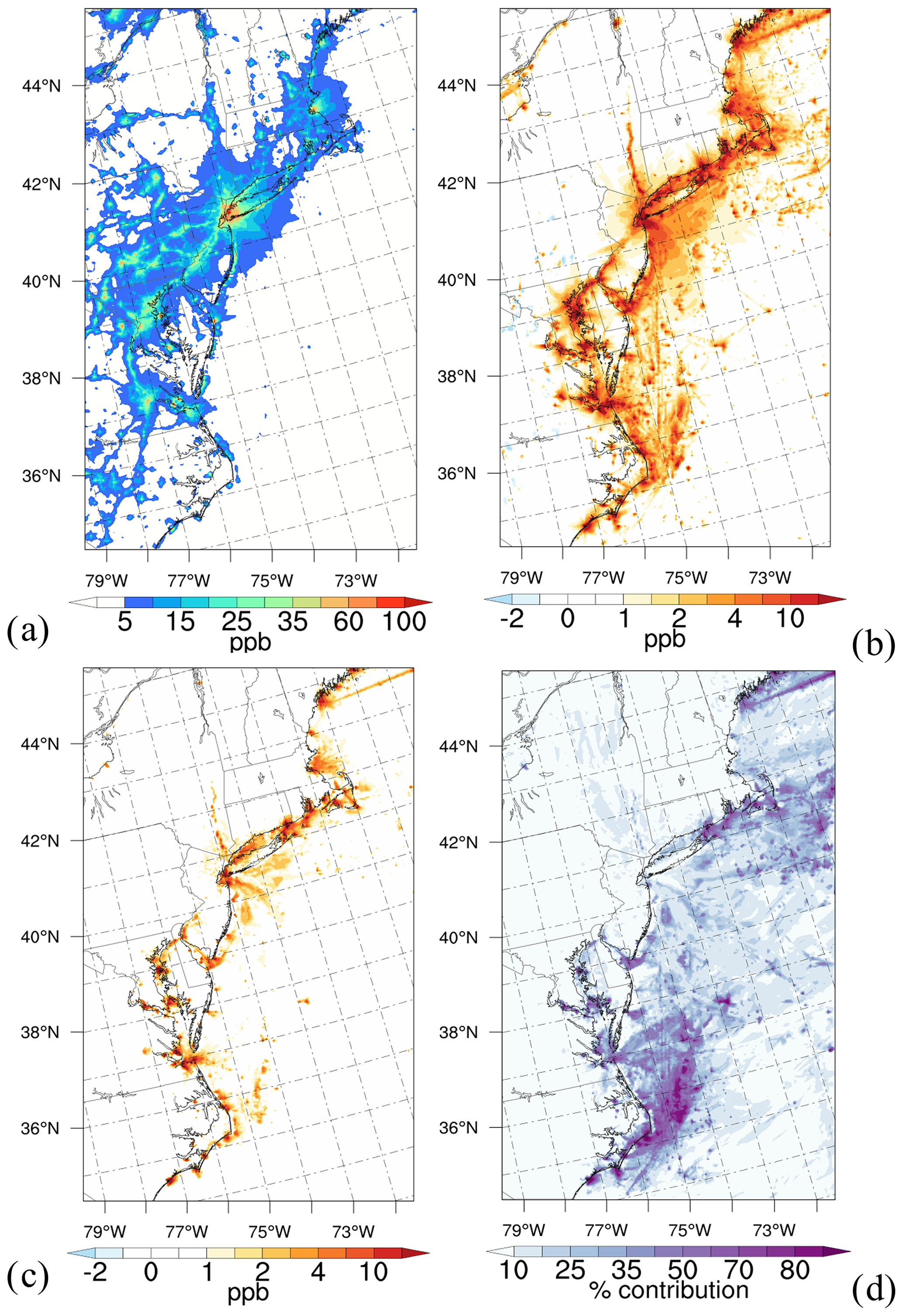
Figure 7 NO₂ concentration results: (a) 98th percentile of 1 h daily maximum NO₂ concentrations with ships (WithShips); (b) maximum contribution of the ships during the simulation period (Eq. 1); (c) differences between the 98th percentile of the 1 h daily maximum between the two scenarios (WithShips minus NoShips); and (d) contribution (in %) of the ships to the 98th percentile of the daily NO₂ maximum.

The maximum contribution of ships to NO₂ concentrations, which is illustrated in Fig. 7b, shows that, in a worst-case scenario, ships contributed to up to ∼50 ppb of NO₂ along the coast and ∼75 ppb over the Atlantic, which is significantly high with respect to the 100 ppb standard. The 3-month highest impact happens near the major ports and shipping routes but stretches to the land and over the ocean.

4.4 Ozone (O₃)

Tropospheric ozone is formed by both naturally occurring and anthropogenic sources. Ozone is not emitted directly into the air, but, in the presence of sunlight, it is created by its precursors: VOCs and NO_x. The rate of ozone production can be limited by either VOCs or NO_x. As a result, a specific location can be either VOC-limited or NO_x-limited. The rate of the production/destruction of O₃ in the atmosphere is different in these regimes. We will further discuss this matter later in this section.

We use 8 h average ozone concentrations for our analysis to maintain consistency with the EPA standards (US EPA, 2022b). We calculated the 8 h averaged ozone values by averaging 8 consecutive hours of O₃ outputs at each hour of the day and storing this information at the start hour (Cohen et al., 1999). For instance, O₃ at 11:00 UTC in a day indicates the time-averaged O₃ concentrations between the hours of 11:00 and 19:00 UTC on that day. Hereafter, we will refer to the 8 h averaged O₃ concentrations simply as O₃ concentrations.

Ambient ozone concentrations are directly affected by temperature, solar radiation, wind speed, and other meteorological factors. As O₃ production is a photochemical reaction, its peak concentrations are found during the daytime when tropospheric ultraviolet radiation in the atmosphere is highest. Because the focus of this study is the daily high episodes of O₃ that are associated with adverse health impacts, we limit our analysis of the maximum impacts to only daytime hours. To select the daytime hours, we considered the 8 h averaged O₃ daily profiles in 10 different locations along the coast from which 4 selected locations are shown in Fig. 8. The lowest concentrations of O₃ are associated with the hours 00:00 to 08:00 UTC (20:00 to 04:00 LT, local time). We eliminated these hours from our analysis to only focus on concentrations during the high episodes. Therefore, we select the hours with peak O₃ concentrations during the 24 h period i.e., 09:00 to 23:00 UTC (05:00 to 19:00 LT).

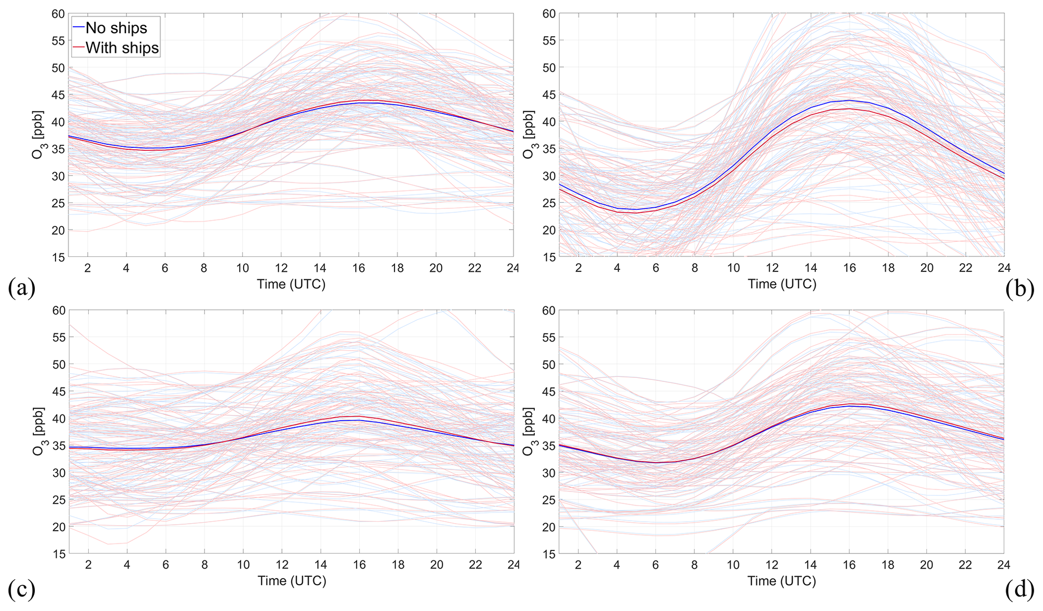
Figure 8 The 8 h average O₃ concentration time series at four different locations along the East Coast from 1 June to 30 August 2018: (a) Atlantic City, New Jersey (NJ); (b) Manhattan, NY; (c) Cape Cod, MA; and (d) Providence, Rhode Island (RI). The thin lines represent the daily time series and the thick lines are the 3-month average profiles; red lines represent the WithShips simulations and blue lines show the NoShips simulations.

We find that, although ship emissions contribute to O₃ enhancement in the region, these emissions reduce O₃ at some urban locations. We detect a significant increase or decrease in O₃ concentrations in the presence of ships depending on whether the location was an NO_x- or VOC-limited area.

The maximum contribution of ships to the O₃ levels over the entire 3-month period is illustrated in Fig. 9c as a worst-case scenario. Over the ocean, the maximum increase is large, up to 8.6 ppb. However, the pollution increase remained primarily offshore and did not significantly impact the coastal areas. O₃ increased by 4–5 ppb at most in parts of North Carolina; Baltimore, MD; and parts of CT and MA. Otherwise, the maximum increase over the land was up to 3.5 ppb. It is important to note that the maximum impact is not necessarily at the time when high-O₃ episodes (from a regulatory perspective) are found. Despite the O₃ increase over the Atlantic, the maximum contribution of ships is negative at the shore where the major ports are built, suggesting that O₃ was destroyed in the presence of the ships. This is due to the complex nature of atmospheric chemistry, where fresh NO emissions from ships scavenge O₃ and reduce its concentrations in urban VOC-limited areas.

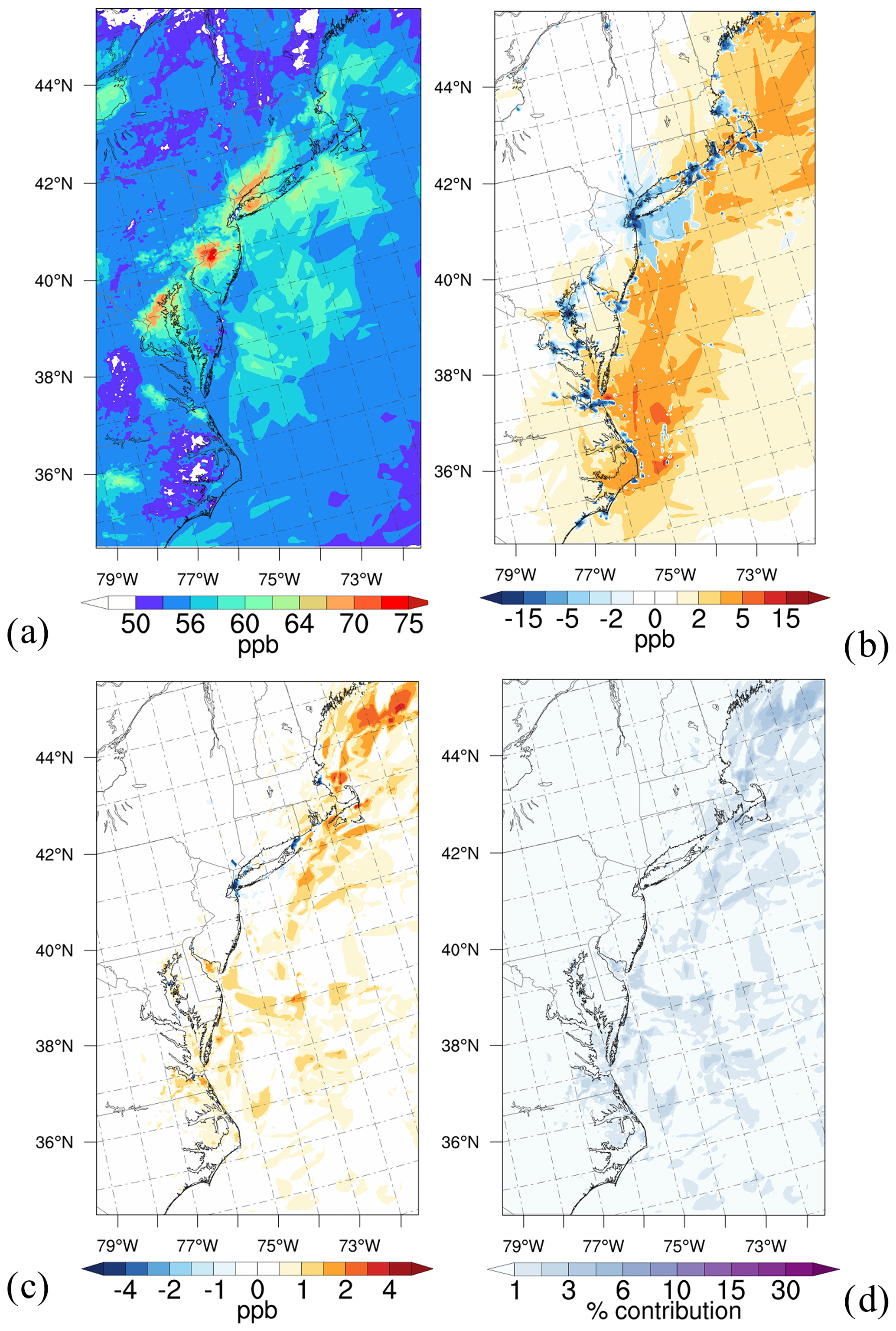
Figure 9 O₃ concentration results: (a) fourth highest 8 h daily maximum O₃ concentrations with ships (WithShips); (b) maximum contribution of the ships during the 3-month simulation period (Eq. 1); (c) differences between the fourth highest 8 h daily maximum between the two scenarios (WithShips minus NoShips); and (d) contribution (in %) of the ships to the fourth highest daily O₃ maximum.

While Fig. 9b is important to understand the worst-case scenario of the shipping impact on O₃ pollution in the region, it does not help to measure the impact of these changes on state compliance with EPA standards. This is because a high impact on O₃ in the worst-case scenario may not correspond to the time of the day when O₃ daily maxima occurred. Therefore, to study the impacts of ship emissions from a policy perspective, it is necessary to explore the impacts on the O₃ design value at every grid cell. For O₃, the EPA defines this standard as the fourth highest 8 h averaged O₃ daily maxima, averaged over a 3-year period, which should not exceed 70 ppb (US EPA, 2022b). As we do not have data for 3 consecutive years, we focus on the fourth highest daily maximum in our study period, the summer of 2018. Hereafter, in this study, we will refer to this value as the O₃ design value. We assume that this value represents the fourth highest daily maximum in the year 2018, as the highest-O₃ episodes are expected to occur during the summer period. Thus, the regions with O₃ concentrations higher than 70 ppb in Fig. 9a are most susceptible to being in non-attainment with the EPA standards; therefore, the impacts of the ships are of higher significance in those regions. Out of all states in the domain, NY, NJ, and MD are the only states that exceed the 70 ppb standard and are likely to be in non-attainment. All other states stay in attainment with the standards defined in Table 2 in either scenario.

From a policy perspective, O₃ design values increased by up to 3.5 ppb in the presence of the ships over the Atlantic Ocean. However, we find a reduction (up to 6.5 ppb) in O₃ concentrations at major ports along the East Coast (Fig. 9c), where fresh NO is emitted by ships into the atmosphere in VOC-limited regions (Fig. 10). In most parts, the major impact of ships remains offshore away from the coastal areas. However, in some regions in MA, RI, CT, ME, VA, NC, and MD, ships contribute to the O₃ increase at the coast, although only MD is likely to be in non-attainment. The highest increase in the O₃ design value inland is found in VA and NC and is up to 2.5 ppb, whereas we note that the fourth highest daily maximum in NY is decreased by 4 ppb in the presence of ships for the reasons discussed later in this section. However, the decrease in O₃ values remains in Manhattan, NY, and is not associated with the parts of Long Island (NY) where O₃ exceeds the standards.

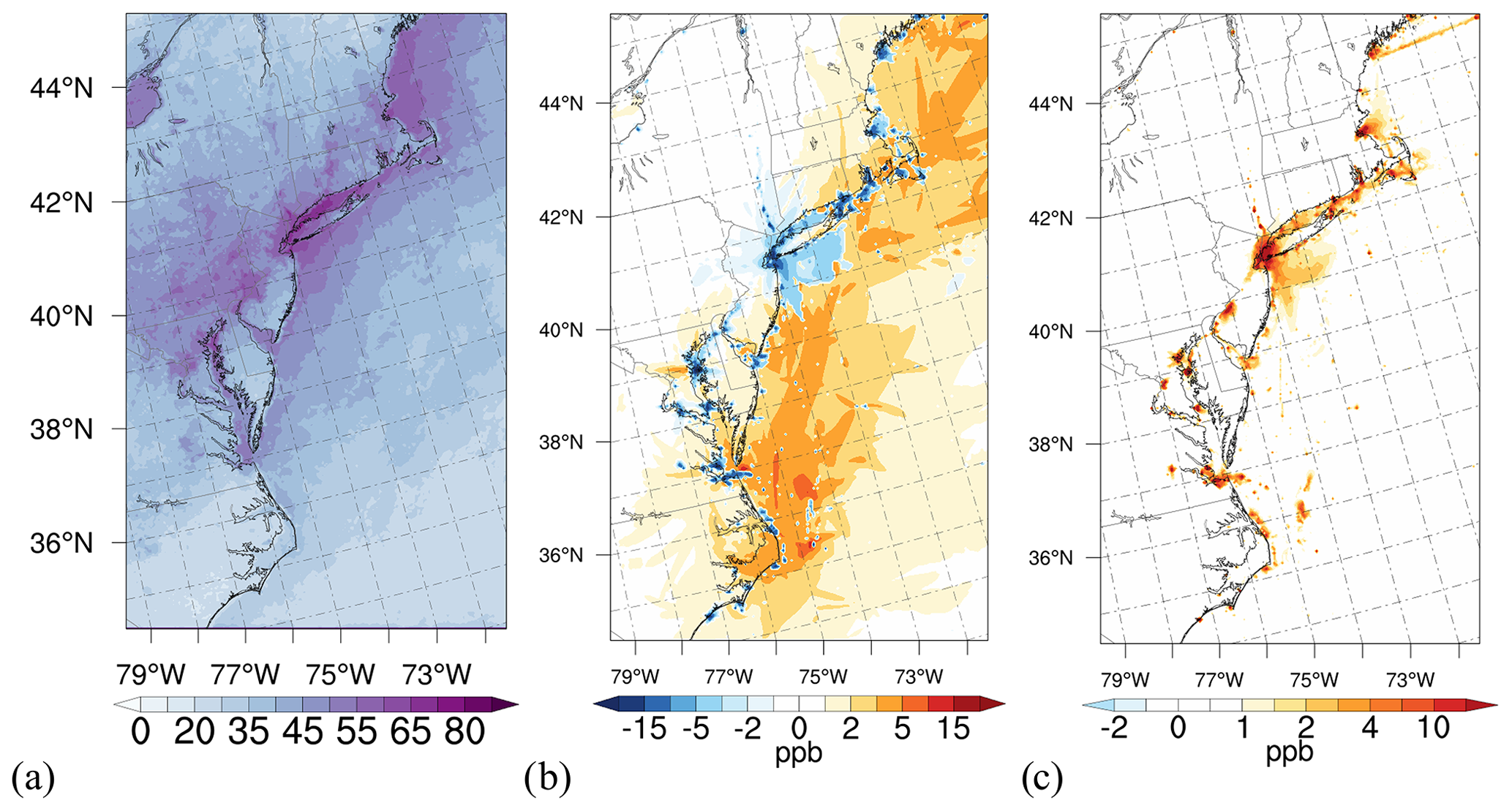
Figure 10 VOC- versus NO_x-limited regime determination: (a) the percentage of the times when $\mathrm{\Delta }{\mathrm{H}}_{\mathrm{2}}{\mathrm{O}}_{\mathrm{2}}/\mathrm{\Delta }{\mathrm{HNO}}_{\mathrm{3}}<\mathrm{0.35}$, as determined in the CAMx model, which is an indication of a VOC-limited regime; (b) maximum contribution of ships to O₃ pollution (Fig. 9c); and (c) maximum contribution of ships to NO pollution.

In the atmosphere, the formation or destruction of ozone depends on the concentrations of both NO_x and VOCs as well as the ratio between them ($\mathrm{VOC}/{\mathrm{NO}}_x$). Transportation is usually associated with high NO_x emissions; therefore, O₃ is generally NO_x-limited in rural areas and VOC-limited in urban areas, with low and high traffic densities, respectively.

In the VOC-limited regions, high concentrations of freshly emitted NO locally scavenge O₃ and lead to the formation of NO₂. Close to the emission sources, this titration process can be considered an ozone sink. In addition, high NO₂ concentrations deflect the initial oxidation step of VOCs by forming other products such as nitric acid (HNO₃), which slows down the formation of O₃ (National Research Council, 1992; Beck et al., 1998). Because of these reactions, an increase in NO leads to a decrease in O₃ in VOC-limited regions.

In CAMx, a VOC-limited regime is defined as occurring when the rate of change of hydrogen peroxide (H₂O₂) is lower compared with the rate of change of HNO₃. A higher $\mathrm{\Delta }{\mathrm{H}}_{\mathrm{2}}{\mathrm{O}}_{\mathrm{2}}/\mathrm{\Delta }{\mathrm{HNO}}_{\mathrm{3}}$ ratio indicates an NO_x-limited regime, whereas a lower $\mathrm{\Delta }{\mathrm{H}}_{\mathrm{2}}{\mathrm{O}}_{\mathrm{2}}/\mathrm{\Delta }{\mathrm{HNO}}_{\mathrm{3}}$ ratio corresponds to a VOC-limited regime. There are other indicators for determining the NO_x-limited or VOC-limited regimes that are discussed in the literature (Li et al., 2022), but we use the $\mathrm{\Delta }{\mathrm{H}}_{\mathrm{2}}{\mathrm{O}}_{\mathrm{2}}/\mathrm{\Delta }{\mathrm{HNO}}_{\mathrm{3}}$ ratio here, as it is used in the CAMx model (Ramboll Environment and Health, 2020).

To understand the formation/destruction of ozone in the presence of ships in our study domain, we calculated the frequency of the VOC-limited regime based on the ratio in every grid cell. Figure 10a illustrates the percentage of the times that a VOC-limited regime occurred in every cell, which is the highest along the coast and in major cities. This indicates that O₃ may be affected by titration when ship emissions are present. We find that the NO concentrations increase along the coast where we detect a decrease in O₃ concentrations (Fig. 10b) and a VOC-limited regime (Fig. 10c).

This finding does not necessarily mean that ships help create better air quality, as a reduction in O₃ is due to a significant increase in other important air pollutants i.e., NO_x concentrations.

4.5 Diurnal cycle of the impacts

In order to examine the diurnal variations in the impact of shipping activities on each of the four pollutants, we generated time series of data representing the daily cycles of changes induced by ships (Fig. 11). To achieve this, we specifically chose four key locations along the eastern coast: Manhattan, NY; Baltimore, MD; Boston, MA; and Norfolk, VA. This selection was deliberate, as these locations encompass large cities as well as major ports, making them suitable representatives for assessing the shipping-related effects on air quality.

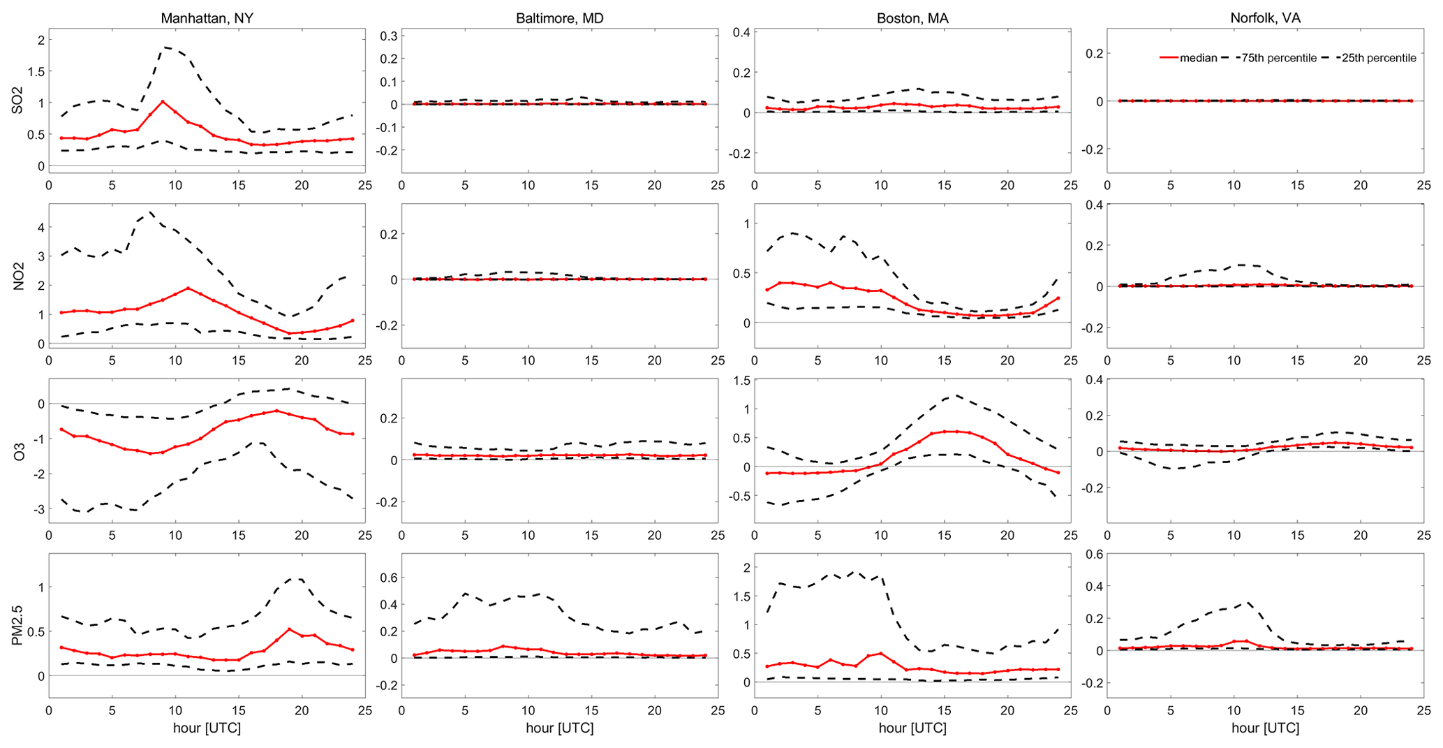
Figure 11 Diurnal cycle of the ship emission impacts on pollutants for (a) SO₂ (ppb), (b) NO₂ (ppb), (c) O₃ (ppb), and (d) PM_2.5 (µg m⁻³). The first through fourth columns represent respective changes in Manhattan, NY; Baltimore, MD; Boston, MA; and Norfolk, VA.

The dashed lines in Fig. 11 are the 25th and 75th percentiles, offering insights into the distribution of the impacts across various days and stations at each simulation hour. In contrast, the solid pink line represents the median impact attributed to the presence of ships. For both NO₂ and SO₂, we observe an increase in concentrations when ships are present at all hours, as evidenced by the positive values of the median diurnal impact. Notably, the most significant impact for NO₂ is observed around 05:00–15:00 UTC (corresponding to 01:00–11:00 LT). For SO₂, we do not detect a clear diurnal pattern across all four locations. The median changes in the O₃ levels show varying patterns across different locations. In Baltimore, MD, and Norfolk, VA, the median impacts on O₃ are minimal. In Manhattan, NY, O₃ levels demonstrate consistent negative changes across all hours, indicating a reduction in the O₃ concentration in the presence of ships, with the most pronounced decrease occurring between 05:00 and 12:00 UTC (equivalent to 01:00 and 08:00 LT, respectively). It is important to note that these values represent the 8 h average O₃ concentrations, meaning that, for instance, 08:00 LT represents the average O₃ levels between the hours of 08:00 and 16:00 LT. Conversely, in Boston, MA, the most significant impacts of ships on O₃ levels are observed between 11:00 and 20:00 UTC (equivalent to 07:00 and 16:00 LT, respectively) and are increased.

PM_2.5 shows a similar diurnal pattern to NO₂: it displays a positive impact (increase in PM_2.5 levels due to ships) for all hours, with the highest impact during ∼ 00:00–12:00 UTC (corresponding to ∼ 20:00 to 08:00 LT), apart from Manhattan, NY, where the highest impacts occur around hour 20:00 UTC (16:00 LT).

It is worth highlighting that the influence of shipping emissions on the four pollutants shown in panels b and c of Figs. 5–9 may be different from the findings in Fig. 11. This divergence arises from our utilization of distinct metrics in these two analyses. In Fig. 11, we base our assessment on median impacts at the four locations, whereas we evaluate the impacts with regard to EPA regulations or under a worst-case scenario in the other figures.

5 Conclusions

Ships emit significant amounts of pollutants within 400 km of the shores. Here, we studied the impact of oceangoing ship emissions on the air quality of the US East Coast. We utilized the WRF-CAMx modeling system to simulate the pollution concentrations in the presence and absence of shipping activities along the East Coast and at the major ports. We used the WRF model to provide the meteorological inputs for the CAMx air quality model for the year 2018, on which the most recent EPA NEI emission inventory is based. We particularly focused on PM_2.5, SO₂, NO₂, and O₃. Overall, we studied the outcomes of every pollutant from two perspectives: (1) from the EPA perspective with respect to the national concentration standards for each specific pollutant and (2) from the perspective of the maximum contribution of ships to that pollutant over 3 months. Our assessment of the CAMx model's performance reveals strong performance with respect to simulating SO₂ levels. The model shows a slight underestimation of O₃ concentrations near the coast and a slight overestimation farther from the shore. Nevertheless, the mean bias error for O₃ is limited to −1.12 ppb. Likewise, the bias in PM_2.5 concentrations remains below 5 µg m⁻³. On the other hand, the model exhibits a noticeable underestimation of NO₂ concentrations, primarily stemming from a positive bias in observations collected in proximity to major roads.

We find that shipping increases the PM_2.5 concentrations across the domain. The 98th percentile daily average PM_2.5 levels increased by 3.2 µg m⁻³ over the ocean and in some coastal areas. However, in a worst-case scenario, ships contribute up to approximately 8.0 µg m⁻³ to PM_2.5 concentrations, only over the Atlantic off the coast of MD and in VA. In addition, we find that ships have a significantly high impact, up to 95 % and 90 %, on the SO₂ concentrations over the Atlantic and inland areas, respectively. This suggests that the CMV sector is one of the highest contributors to SO₂ levels in the region. The shipping contribution to SO₂ levels was up to 45 ppb over coastal regions. Ship emissions also impacted the NO₂ design value by up to 34 ppb. In addition, our simulation results show that the impact of ship emissions on O₃ concentrations is not uniform, meaning that maritime shipping affects ozone pollution in both positive and negative ways. Although O₃ concentrations increase significantly in the presence of ships (up to 8.6 ppb) over the ocean, they decrease by up to ∼6.5 ppb in coastal areas with major cities and major ports. To understand the reasons behind the O₃ reduction in the presence of ships, we analyzed the $\mathrm{\Delta }{\mathrm{H}}_{\mathrm{2}}{\mathrm{O}}_{\mathrm{2}}/\mathrm{\Delta }{\mathrm{HNO}}_{\mathrm{3}}$ ratio in the region, which is used to determine NO_x-limited or VOC-limited ozone production, as well as changes in NO concentrations, as they play a significant role in O₃ formation and destruction. We found that ships emit significant amounts of fresh NO into the atmosphere, which then helps scavenge O₃ in VOC-limited regimes. As a result, with higher NO concentrations in the atmosphere produced by ship emissions, O₃ is destroyed in major cities and urban areas. By contrast, over the ocean (an NO_x-limited regime), excessive NO_x emissions due to ships contribute to the formation of O₃ and, therefore, an enhancement of O₃ concentrations. It is important to note that the destruction of O₃ by ship emissions in major cities does not necessarily mean that the ships create better air quality, as a decrease in O₃ is a consequence of a significant increase in other pollutants like NO. The diurnal cycle in the impact of shipping emissions across four major cities shows different patterns for different locations. For instance, the highest impacts on O₃, occur at different times for different locations. PM_2.5 and NO₂, however, experience the highest changes in the early morning at most locations. On the other hand, we do not detect consistent patterns for changes in SO₂.

Overall, the majority of the time, due to the dominant southwesterly wind direction in the region, the impacts on different pollutants remained spatially confined offshore. However, in some coastal areas near the major ports, the impacts were significant.