the Creative Commons Attribution 4.0 License.
the Creative Commons Attribution 4.0 License.
 | 05 Dec 2023
Investigation of spatial and temporal variability in lower tropospheric ozone from RAL Space UV–Vis satellite products
Richard J. Pope
Brian J. Kerridge
Richard Siddans
Barry G. Latter
Martyn P. Chipperfield
Wuhu Feng
Matilda A. Pimlott
Sandip S. Dhomse
Christian Retscher
Richard Rigby
Ozone is a potent air pollutant in the lower troposphere and an important short-lived climate forcer (SLCF) in the upper troposphere. Studies using satellite data to investigate spatiotemporal variability of troposphere ozone (TO3) have predominantly focussed on the tropospheric column metric. This is the first study to investigate long-term spatiotemporal variability in lower tropospheric column ozone (LTCO3, surface–450 hPa sub-column) by merging multiple European Space Agency–Climate Change Initiative (ESA-CCI) products produced by the Rutherford Appleton Laboratory (RAL) Space. We find that in the LTCO3, the degree of freedom of signal (DOFS) from these products varies with latitude range and season and is up to 0.8, indicating that the retrievals contain useful information on lower TO3. The spatial and seasonal variation of the RAL Space products are in good agreement with each other, but there are systematic offsets of up to 3.0–5.0 DU between them. Comparison with ozonesondes shows that the Global Ozone Monitoring Experiment (GOME-1, 1996–2003), the SCanning Imaging Absorption spectroMeter for Atmospheric CartograpHY (SCIAMACHY, 2003–2010) and the Ozone Monitoring Instrument (OMI, 2005–2017) have stable LTCO3 records over their respective periods, which can be merged together. However, GOME-2 (2008–2018) shows substantial drift in its bias with respect to ozonesondes. We have therefore constructed a robust merged data set of LTCO3 from GOME-1, SCIAMACHY and OMI between 1996 and 2017. Comparing the LTCO3 differences between the 1996–2000 and 2013–2017 5-year averages, we find sizeable positive increases (3.0–5.0 DU) in the tropics/sub-tropics, while in the northern mid-latitudes, we find small-scale differences in LTCO3. Therefore, we conclude that there has been a substantial increase in tropical/sub-tropical LTCO3 during the satellite era, which is consistent with tropospheric column ozone (TCO3) records from overlapping time periods (e.g. 2005–2016).
Please read the corrigendum first before continuing.
-
Notice on corrigendum
The requested paper has a corresponding corrigendum published. Please read the corrigendum first before downloading the article.
-
Article
(13348 KB)
-
The requested paper has a corresponding corrigendum published. Please read the corrigendum first before downloading the article.
- Article
(13348 KB) - Full-text XML
- Corrigendum
- BibTeX
- EndNote


Tropospheric ozone (TO3) is a short-lived climate forcer (SLCF) and is the third most important greenhouse gas (GHG; e.g. Myhre et al., 2013). TO3 is also a hazardous air pollutant with adverse impacts on human health (WHO, 2018) and the biosphere (e.g. agricultural and natural vegetation; Sitch et al., 2007). Since the pre-industrial (PI) period, anthropogenic activities have increased the atmospheric loading of ozone (O3) precursor gases, most notably nitrogen oxides (NOx) and methane (CH4), resulting in a substantial increase in TO3 of 25 %–50 % since 1900 (Gauss et al., 2006; Lamarque et al., 2010; Young et al., 2013). The PI to present day (PD) radiative forcing (RF) from TO3 is estimated by the Intergovernmental Panel on Climate Change (IPCC) to be 0.47 W m−2 (Forster et al., 2021) with an uncertainty range of 0.24–0.70 W m−2.
During the satellite era, with a number of missions since 2000, extensive records of TO3 have been produced, e.g. by the European Space Agency Climate Change Initiative (ESA-CCI; ESA, 2019). However, the large overburden of stratospheric O3, coupled with the different vertical sensitivities and sources of error associated with observations in different wavelength regions (e.g. Eskes and Boersma, 2003; Ziemke et al., 2011; Miles et al., 2015), contributes to large-scale spatiotemporal inconsistencies between the records (Gaudel et al., 2018). Various studies (e.g. Heue et al., 2016; Pope et al., 2018; Ziemke et al., 2019) analysing TO3 trends usually focussed on one or two instruments. The work by Gaudel et al. (2018) was part of the Tropospheric Ozone Assessment Report (TOAR), which represented a large global effort to understand spatiotemporal patterns and variability in TO3. Gaudel et al. (2018) analysed ozonesondes and multiple polar-orbiting–nadir-viewing satellite products and reported large-scale discrepancies in the spatial distribution, magnitude, direction and significance of the tropospheric column ozone (TCO3) trends. While the satellite records did cover slightly different time periods, they were unable to provide any definitive reasons for these discrepancies beyond briefly suggesting that differences in measurement techniques and retrieval methods were likely to be causing the observed spatial inconsistencies. Another factor introducing inconsistencies is the assumed tropopause height for the different products. Some products used the World Meteorological Organization (WMO) definition of “the first occurrence of the 2 K km−1 lapse rate”, while some others, for example, integrated the 0–6 and 6–12 km sub-columns to derive the tropospheric column. The use of different a priori products within the retrieval scheme will have also provided inconsistencies.
The vertical sensitivity of each product (function of measurement technique and retrieval methodology) used by Gaudel et al. (2018) has a substantial impact on which part of the troposphere (and stratosphere) the O3 signal is weighted towards. The vertical sensitivity can be referred to as the “averaging kernel” (AK), which provides the relationship between perturbations at different levels in the retrieved and true profiles (Rodgers, 2000; Eskes and Boersma, 2003). As the instruments' vertical sensitivities differ, they are likely to be influenced differently by processes controlling TO3 temporal variability in different layers of the troposphere (e.g. lower troposphere influenced more by precursor emissions vs. the upper troposphere subject more to the influence from stratospheric–tropospheric exchange). Therefore, the differing vertical sensitivities, and thus the TO3 they are retrieving, could be driving the inconsistencies in reported TCO3 trends between products.
While many studies have previously focussed on TCO3 (e.g. Gaudel et al., 2018; Ziemke et al., 2019), several nadir-viewing ultraviolet–visible (UV–Vis) sounders can retrieve TO3 between the surface to 450 hPa (i.e. lower tropospheric column O3, LTCO3). The retrieval scheme from the Rutherford Appleton Laboratory (RAL) Space exploits information from the O3 Huggins bands (325–335 nm), as well as the Hartley band (270–307 nm), to retrieve high-quality LTCO3 and was selected for the ESA-CCI and EU Copernicus Climate Change Service. As a result, the RAL Space LTCO3 products (and equivalent from other providers) are valuable resources to investigate global and regional O3-related air quality (e.g. Richards et al., 2013; Pope et al., 2018; Russo et al., 2023).
In this study, we explore the spatiotemporal variability of LTCO3 from several UV–Vis sounders produced by RAL Space. While Gaudel et al. (2018) used a range of UV–Vis and infrared (IR) TCO3 products, including the RAL Space Ozone Monitoring Instrument (OMI) product, we focus here on several RAL Space UV–Vis products. Here, we aim to explore the consistencies between them, their vertical sensitivities, LTCO3 stability against ozonesonde records and suitability for long-term trend analysis. In our article, Sect. 2 discusses the satellite/ozonesonde data sets used, Sect. 3 presents are results, while Sect. 4 summarises our conclusions and discussion points.
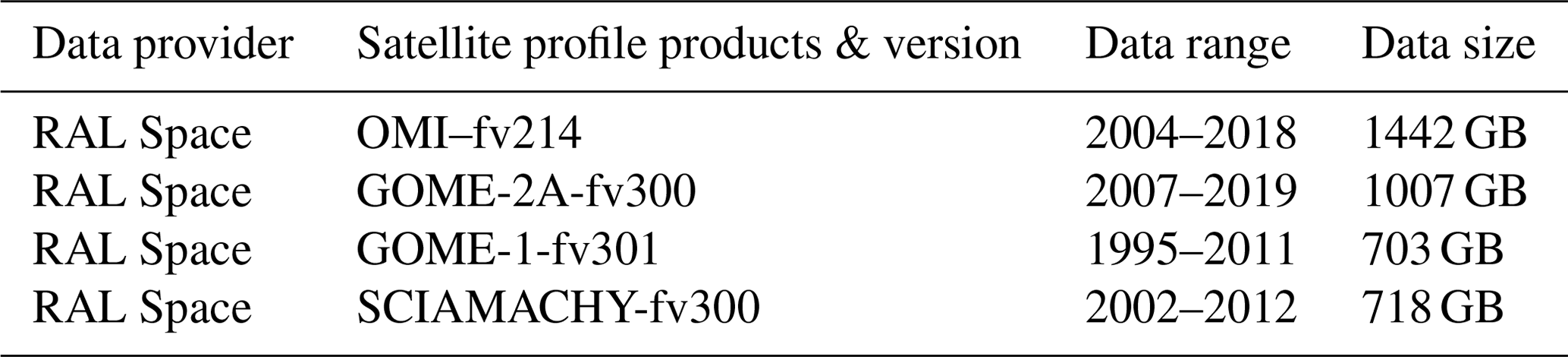
Table 1List of RAL Space level-2 satellite ozone profile data sets.
2.1 Data sets
The four RAL Space UV–Vis satellite products investigated here are from OMI, the Global Ozone Monitoring Experiment (GOME-1), GOME-2 and the SCanning Imaging Absorption spectroMeter for Atmospheric CartograpHY (SCIAMACHY), all of which were developed as part of the ESA-CCI project (Table 1). GOME-1, GOME-2, SCIAMACHY and OMI flew on ESA's ERS-2, MetOp-A, ENVISAT and NASA's Aura satellites in sun-synchronous low Earth polar orbits with local overpass times of 10:30, 09:30, 10:00 and 13:30, respectively. They are all nadir viewing with spectral ranges which include the 270–350 nm range used for ozone profile retrieval. The spatial footprints of the respective instruments at nadir are 320 km × 40 km, 80 km × 40 km, 240 km × 30 km and 24 km × 13 km (Boersma et al., 2011; Miles et al., 2015; Shah et al., 2018). The scheme established by RAL Space to retrieve height-resolved O3 profiles with tropospheric sensitivity (Miles et al., 2015) was applied to all of these satellite instruments. The scheme is based on the optimal estimation (OE) approach of Rogers et al. (2000) and provides state-of-the-art retrieval sensitivity to lower TO3, which is described in detail by Miles et al., (2015) and by Keppens et al., (2018). The differences between the retrieval versions (i.e. fv214 and fv300) in Table 1 are primarily linked to the instrument types where GOME-1, GOME-2 and SCIAMACHY are across-track scanning instruments while OMI uses a 2-D array detector. For this work, the data were filtered for good-quality retrievals whereby the geometric cloud fraction was <0.2, the lowest sub-column O3 value was >0.0, the solar zenith angle , the convergence flag = 1.0 and the normalised cost function was <2.0. These filters also remove OMI pixels influenced by the OMI row anomaly (Torres et al., 2018), so there is reduced OMI data coverage over the record. However, we find this has minimal impact on our results with substantial proportions of data (e.g. millions of retrievals per year at the start and end of the OMI record) available for analysis in our study.
2.2 Ozonesondes and application of satellite averaging kernels
To help understand the impact of the satellite AKs on retrieved LTCO3 and stability of the satellite instruments listed in Table 1 over time, we use ozonesonde data between 1995 and 2019 from the World Ozone and Ultraviolet Radiation Data Centre (WOUDC), the Southern Hemisphere ADditional OZonesondes (SHADOZ) project, and from the National Oceanic and Atmospheric Administration (NOAA). Keppens et al. (2018) undertook a detailed assessment of the ESA-CCI TO3 data sets, including the RAL UV–Vis profile data sets used in this study (mostly older versions though) using ozonesondes. They found that the RAL LTCO3 products typically had a positive bias of about 40 %, apart from OMI which was closer to 10 %. On the global scale, tropospheric drift in GOME-1 and OMI over time was approximately −5 % and 10 % per decade, respectively. However, GOME-2 and SCIAMACHY had significant tropospheric drift trends of approximately 40 % per decade. The recent Copernicus Product Quality Assessment Report (PQAR) Ozone Products Version 2.0b (Copernicus, 2021) undertook a more recent assessment of nadir ozone profiles using the level 3 products from RAL listed in Table 1. They found that in the troposphere, OMI/GOME-1 and SCIAMACHY/GOME-2 had biases of −20 % and 10 %. GOME-1 tropospheric drift was deemed to be insignificant (−10 % to 5 % per decade), while GOME-2 and SCIAMACHY had a significant drift of 30 % and 20 % per decade, respectively. OMI also had an insignificant tropospheric drift of 10 % per decade.
In this study, for comparisons between ozonesonde profiles and satellite retrievals, each ozonesonde profile was spatiotemporally co-located to the closest satellite retrieval. Here, all the retrievals within 6 h of the ozonesonde launch were subsampled, and then the closest retrieval in space (i.e. within 500 km) was taken for the final co-located one. Therefore, there was one satellite retrieval for every ozonesonde profile to help reduce the spatiotemporal sampling difference errors. Here, ozonesonde O3 measurements were rejected if the O3 or pressure values were unphysical (i.e. <0.0), if the O3 partial pressure >2000.0 mPa or the O3 value was set to 99.9, and whole ozonesonde profiles were rejected if at least 50 % of the measurements did not meet these criteria. These criteria are similar to those applied by Keppens et al. (2018) and Hubert et al. (2016). To allow for direct like-for-like comparisons between the two quantities, accounting for the vertical sensitivity of the satellite, the instrument AKs were applied the ozonesonde profiles. Here, each co-located ozonesonde profile (in volume mixing ratio) was used to derive ozone sub-columns (in number density) on the satellite pressure grid. The application of the AKs for the UV–Vis instruments was done using Eq. (1):
where sondeAK is the modified ozonesonde sub-column profile (Dobson units, DU), AK is the averaging kernel matrix, sondeint is the sonde sub-column profile (DU) on the satellite pressure grid and apr is the a priori sub-column amount (DU). Here, the ozonesonde profiles, on its original pressure grid (typically in units of ppbv or mPa), are converted into ozone sub-columns between each pair of measurement levels. These sub-columns are then aggregated up to the larger sub-columns (e.g. the LTCO3 range is between the surface and 450 hPa) on the coarser satellite pressure grid.
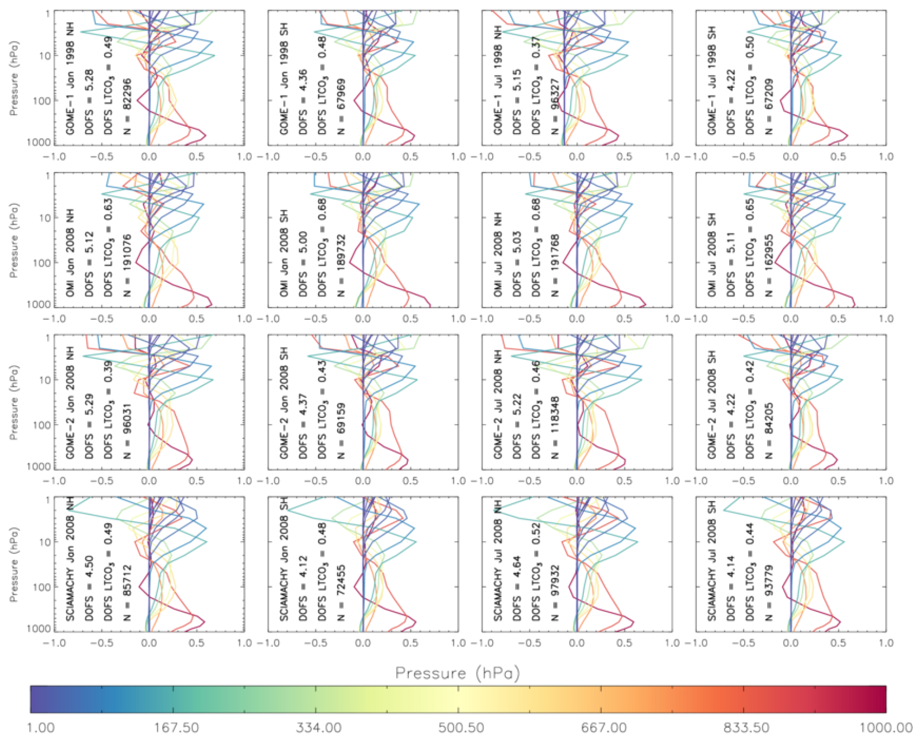
Figure 1Average averaging kernels (AKs) for the instruments listed in Table 1 for the Northern Hemisphere and Southern Hemisphere (restricted to ± 60∘ N/S) in January and July of 2008 (1998 for GOME-1). The average degree of freedom of signal (DOFS) is shown as is DOFS LTCO3, which represents the DOFS in the lower tropospheric column ozone (LTCO3). N represents the number of retrievals in each average AK.
3.1 Satellite vertical sensitivity
Figure 1 represents average AKs for all the instruments listed in Table 1 for 2008 (1998 for GOME-1) in the Northern Hemisphere (NH) and Southern Hemisphere (SH) between the Equator and 60∘ S and N. Of the four RAL Space products, OMI O3 profiles appear to contain the most information with a degree of freedom of signal (DOFS) of 5.0 or above for the full atmosphere. Here, the DOFS represents the number of independent pieces of information on the vertical profile in the retrieval (i.e. the sum of the AK diagonal). SCIAMACHY has the lowest sensitivity with average DOFS ranging between 4.12 and 4.64. The DOFS tends to be larger in NH for all the products, though there is no clear pattern in the seasonality (i.e. January vs. July). In terms of LTCO3, OMI again has greater sensitivity than the others with average hemispheric and seasonal DOFS ranging between 0.63 and 0.68. For GOME-1 (GOME-2), the LTCO3 DOFS ranges between 0.37 and 0.50 (0.39 and 0.46). SCIAMACHY LTCO3 DOFS ranges between 0.44 and 0.52. Therefore, while SCIAMACHY has the lowest overall information on the full atmospheric ozone, it has reasonably good information in the LTCO3, as do the other instruments. These results are robust given the large number of retrievals (N) that have been used to derive the average AKs (i.e. N>65 000 in all cases).
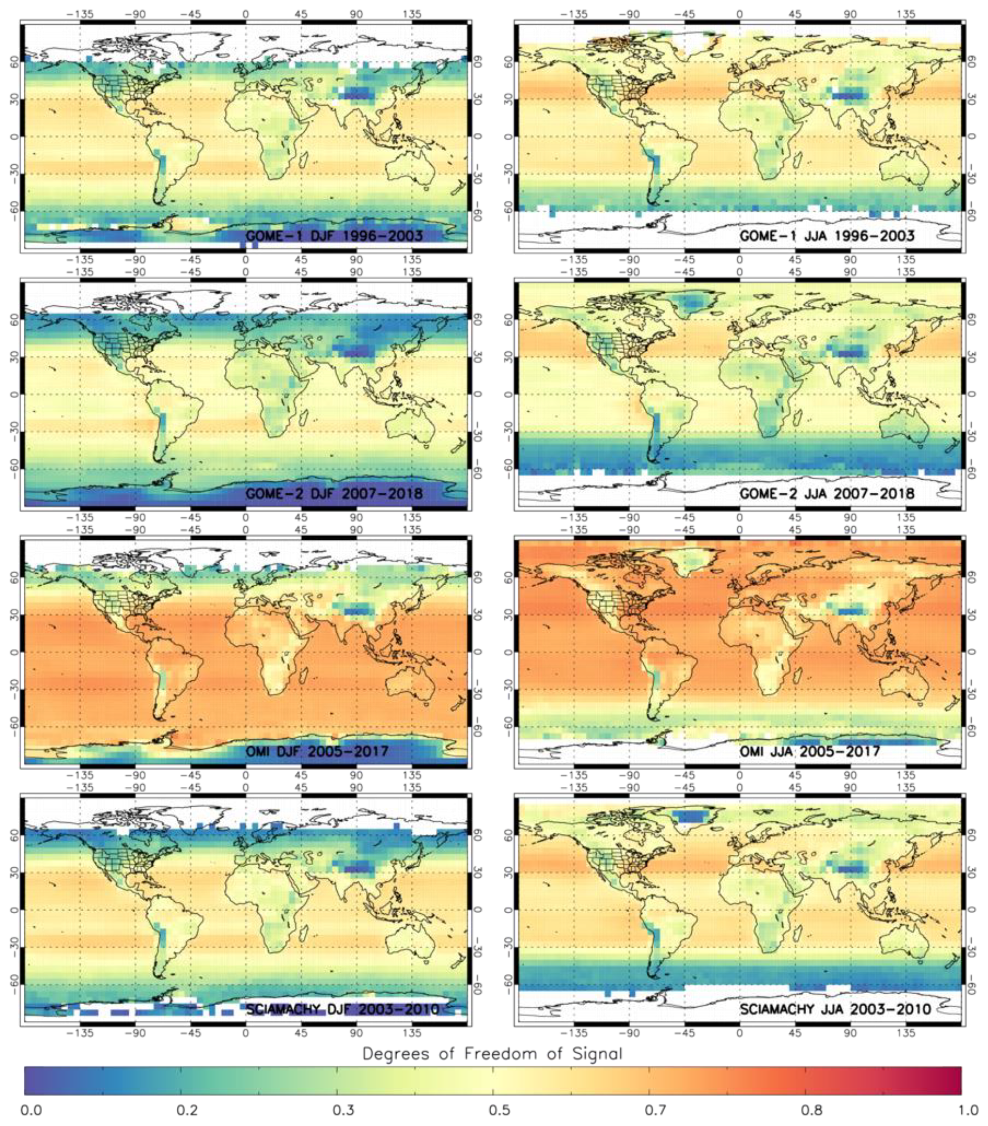
Figure 2Seasonal distributions of LTCO3 degrees of freedom of signal (DOFS) in DJF and JJA for GOME-1, GOME-2, OMI and SCIAMACHY averaged over the full record for each instrument.
While Fig. 1 provides spatial average information on LTCO3 DOFS, Fig. 2 shows spatial maps for December–January–February (DJF) and June–July–August (JJA) over the respective instrument records. The largest LTCO3 DOFS occur over the ocean ranging between approximately 0.4 and 0.6 for GOME-1, GOME-2 and SCIAMACHY, while OMI has larger ocean values between 0.7 and 0.8. Over land, the LTCO3 DOFS tend to be lower and between 0.3 and 0.5 for GOME-1, GOME-2 and SCIAMACHY. Again, OMI has larger values on land of between 0.4 and 0.7. Depending on the hemispheric season, the summertime (JJA in NH and DJF in SH) LTCO3 DOFS is larger for each instrument. Overall, OMI (GOME-2) retrievals contain the largest (lowest) amount of information on LTCO3.
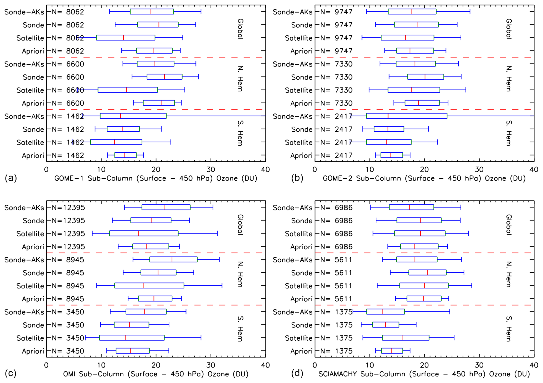
Figure 3Box and whisker distributions of LTCO3 from satellite, a priori, ozonesonde (Sonde) and ozonesonde with AKs applied (Sonde–AKs) for co-located samples (i.e. satellite and ozonesonde profiles co-located within 6 h and 500 km). This is done for GOME-1 (a), GOME-2 (b), OMI (c) and SCIAMACHY (d) on a global, southern hemispheric and northern hemispheric basis over their respective records. Dashed red lines separate the box and whisker distributions for each region. The red, green and blue vertical lines represent the 50th, 25th and 75th, and 10th and 90th percentiles, respectively. N represents the sample size.
The impact of the satellite vertical sensitivity is further investigated by co-locating the products with the merged ozonesonde data set, over their respective mission periods (globally and in the NH and SH) and the AKs applied to assess the impact on the ozonesondes (Fig. 3). For all the instruments, there are suitable samples sizes (N>1000 in all cases) of co-located retrievals and derived ozonesonde LTCO3. In the case of GOME-1, the global distribution has a 25th–75th percentile (25_75 %) range of approximately 8.0 to 20.0 DU and a median of 14.0 DU. The a priori 25_75 % range and median values are 16.0 to 22.0 and 19.0 DU. These substantial differences between retrieved and a priori values confirm there is sensitivity in the GOME-1 retrieval to lower tropospheric ozone. It can be seen from Eq. (1) that if a satellite instrument had perfect sensitivity at all levels (i.e. AK = 1), there would be no change in co-located ozonesonde LTCO3 distribution when the AKs are applied. However, given AK values are less than 1.0 in Fig. 1, leading to the DOFS of approximately 0.5, there is a shift in the median value towards the a priori from approximately 21.0 to 19.0 DU. The corresponding ozonesonde 10th–90th percentile (10_90 %) range of 13.0 to 26.0 DU expanded to 12.0 to 27.0 DU. Therefore, the application of the AKs to the ozonesondes actually increases the range of observed values. In the NH, the GOME-1 median (25_75 % range) is 14.0 (4.0–24) DU, while the a priori median (25_75 % range) is 21.0 (18.0–23.0) DU. The ozonesonde median (25_75% range) is 22.0 (19.0–25.0) DU, while application of the AKs yields values of 19.0 (16.0–24.0) DU. In the SH, the GOME-1 median (25_75 % range) is 12.0 (8.0–17.0) DU, while the a priori median (25_75 % range) is 14.0 (12.0–16.0) DU. The ozonesonde median (25_75 % range) is 12.0 (11.0–17.0) DU, while application of the AKs yields values of 12.0 (6.0–40.0) DU. In comparison, GOME-2 shows a similar response though the shift in LTCO3 value between the a priori and satellite is smaller. This makes sense given the lower vertical sensitivity of GOME-2. In the SH, the application of the AKs to the ozonesondes yields a very large range in the percentiles. It is likely that the South Atlantic Anomaly (SAA – i.e. where charged particles directly impact UV detectors increasing dark-current noise, which in turn reduces the number of retrievals from all UV sensors, notably both GOME-1 and GOME-2; Keppens et al., 2018), given the typically larger values and signal corruption, is driving the large response in the ozonesonde+AKs range.
For OMI, the global distribution has a median (25_75 % range) of 17.0 (13.0–25.0) DU yielding a substantial shift from the a priori median (25_75 % range) of 18.0 (16.0–22.0) DU. In the NH, the satellite median (25_75 % range) is 18.0 (13.0–25.0) DU and the a priori median (25_75 % range) value is 20.0 (17.0–23.0) DU. In the SH, the satellite median (25_75 % range) is 14.0 (10.0–22.0) DU and the a priori median (25_75 % range) value 15.0 (13.0–19.0) DU. When the AKs are applied to the ozonesondes there is typically an increase in the median LTCO3 and range by approximately 3.0–4.0 DU. This increase in LTCO3 when the OMI AKs are applied to the ozonesondes contrasts with the other satellite instruments. While the vertical smearing from the stratosphere would intuitively be expected to increase the tropospheric layer retrieval, and thus the AK adjustment to decrease the ozonesonde value, in the case of OMI there is a negative excursion in the AKs into the lowermost stratosphere (see Fig. 1), so the opposite occurs. For SCIAMACHY, a similar relationship occurs to that of GOME-1 and GOME-2 with a shift of the satellite LTCO3 median away from the a priori by 1.0–3.0 DU and an increase the in 25_75 % range by 10.0–15.0 DU. Apart from the SH, the application of the AKs to the ozonesondes shifts the LTCO3 median by 2.0–3.0 DU, but the 25_75 % range remains similar. Overall, there is shift in the satellite LTCO3 median value away from the a priori with an increase in the 25_75 % and 10_90 % ranges. A similar pattern occurs in multiple cases between the ozonesondes and the ozonesondes + AKs. Therefore, all the instruments have reasonable vertical sensitivity in LTCO3 with substantial perturbations from the a priori and to the satellite LTCO3 distribution.
3.2 Lower tropospheric column ozone seasonality
Multiple studies have investigated the seasonality of TO3 from space observing large biomass-burning- and lightning-induced O3 in the South Atlantic (Ziemke et al., 2006, 2011; Pope et al., 2020), enhanced summertime TO3 over the Mediterranean (Richards et al., 2013), TO3 over large precursor regions such as China and India (Verstraeten et al., 2015), and the enriched northern hemispheric background O3 during springtime (Ziemke et al., 2006). Here, we compare the long-term seasonal (DJF and JJA) spatial distributions of RAL Space LTCO3 products (Fig. 4).
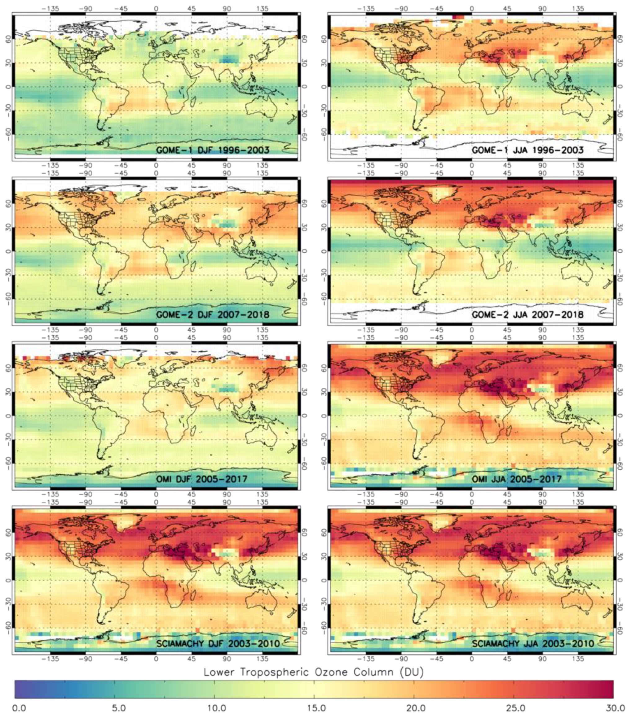
Figure 4Seasonal distributions of LTCO3 in December–January–February (DJF) and June–July–August (JJA) for GOME-1, GOME-2, OMI and SCIAMACHY averaged over the full record for each instrument.
OMI and GOME-2 LTCO3 have regions of consistency (e.g. JJA NH enhanced background TO3, between 20.0 DU and 30.0 DU, and the Mediterranean TO3 peak, >25.0 DU), but the SAA interferes with the signal of the biomass-burning-induced secondary O3 formation from Africa and South America. However, for OMI, this ozone plume ranges between 23.0 and 27.0 DU (18.0 and 20.0 DU) in DJF (JJA). There are also clear LTCO3 hotspots over anthropogenic regions (e.g. eastern China and northern India) peaking at over 25.0 DU in JJA.
The GOME-1 LTCO3 spatial patterns are consistent with that of OMI and GOME-2, but there is a systematic low bias relative to OMI and GOME-2 in the absolute LTCO3 of 3.0 to 7.0 DU, depending on geographical location (e.g. 20.0–22.0 DU over northern India for GOME-2 and OMI, while 16–18 DU for GOME-1). These differences in the GOME-1 and GOME-2/OMI LTCO3 seasonal averages are likely to be at least partly due to underlying LTCO3 tendencies between the respective instrument time periods. This is investigated further in Sect. 3.4. The SCIAMACHY spatial pattern and absolute LTCO3 values are more consistent with OMI and GOME-2. Moreover, SCIAMACHY shows limited sensitivity to the SAA and resolves the biomass burning/lightning O3 sources detected by OMI over South America, the South Atlantic and Africa (18.0–20.0 DU in JJA). However, especially in the NH in DJF, there appears to be regions of latitudinal banding in the LTCO3 spatial patterns (e.g. 0–30∘ N), which are not observed (or to the same extent) as the other UV–Vis sounders. Overall, GOME-2 and OMI are in good agreement spatially and seasonally with similar absolute LTCO3 values. In DJF and JJA, OMI appears to be 2.0–3.0 DU lower and larger than GOME-2, respectively. This is reasonable given the similar temporal records they cover (2005–2017 vs. 2007–2018). SCIAMACHY has similar spatial–seasonal patterns but has systematically larger (3.0–5.0 DU) DJF values in comparison to OMI and GOME-2.
The satellite LTCO3 seasonality is consistent with that of the ozonesondes. Here, the median (25th percentile, 75th percentile) ozonesonde LTCO3 values for the NH in DJF, NH in JJA, SH in DJF and SH in JJA are 18.0 (15.7, 20.0) DU, 20.8 (16.7, 24.6) DU, 10.8 (8.2, 14.8) DU and 14.4 (12.1, 16.3) DU, respectively. Therefore, the NH LTCO3 values are larger than those in the SH, and the JJA LTCO3 values are larger than the DJF equivalent, all of which are consistent with the four instrument LTCO3 seasonal distributions.
3.3 Satellite instrument temporal stability
For accurate assessment of satellite LTCO3 temporal variability, there needs to be insignificant drift over time, whereas bias which is constant over time can be tolerated. The most appropriate data set with which to assess satellite long-term drifts is that of the ozonesonde record, albeit that it has certain limitations potentially including temporal changes in accuracy (Stauffer et al., 2020) as well as geographical coverage. Figure 5 shows annual time series of the satellite ozonesonde (with AKs applied) median biases for three latitude bands: 90–30∘ S, 30∘ S–30∘ N and 30–90∘ N. The hatched pixels show where the biases are non-substantial, defined as the 25_75 % difference range intersecting with zero. For GOME-1, the mean bias (MB) is −5.34, −3.21 and −0.90 DU for the three regions, respectively. For the 30–90∘ N region, several years show substantial biases of −6.0 to −3.0 DU. The two other latitude bands have few substantial years, but in the tropical band, both 2002 and 2003 show substantial biases of approximately −5.0 DU. To assess the stability of the instruments with time, a simple linear least-squares fit was performed with regional trends of −0.32, and −0.03 DU yr−1. A substantial trend (shown by an asterisk) has a p value < 0.05 as defined as (e.g. Pope et al., 2018), where M and σM are the linear trend and trend uncertainty, respectively. While the 30–90∘ N region had a sizable systematic bias, it was stable with time, as was the bias for the 90–30∘ S region. However, the 2002 and 2003 biases in the 30∘ S–30∘ N region gave rise to a substantial drift in the GOME-1 record.
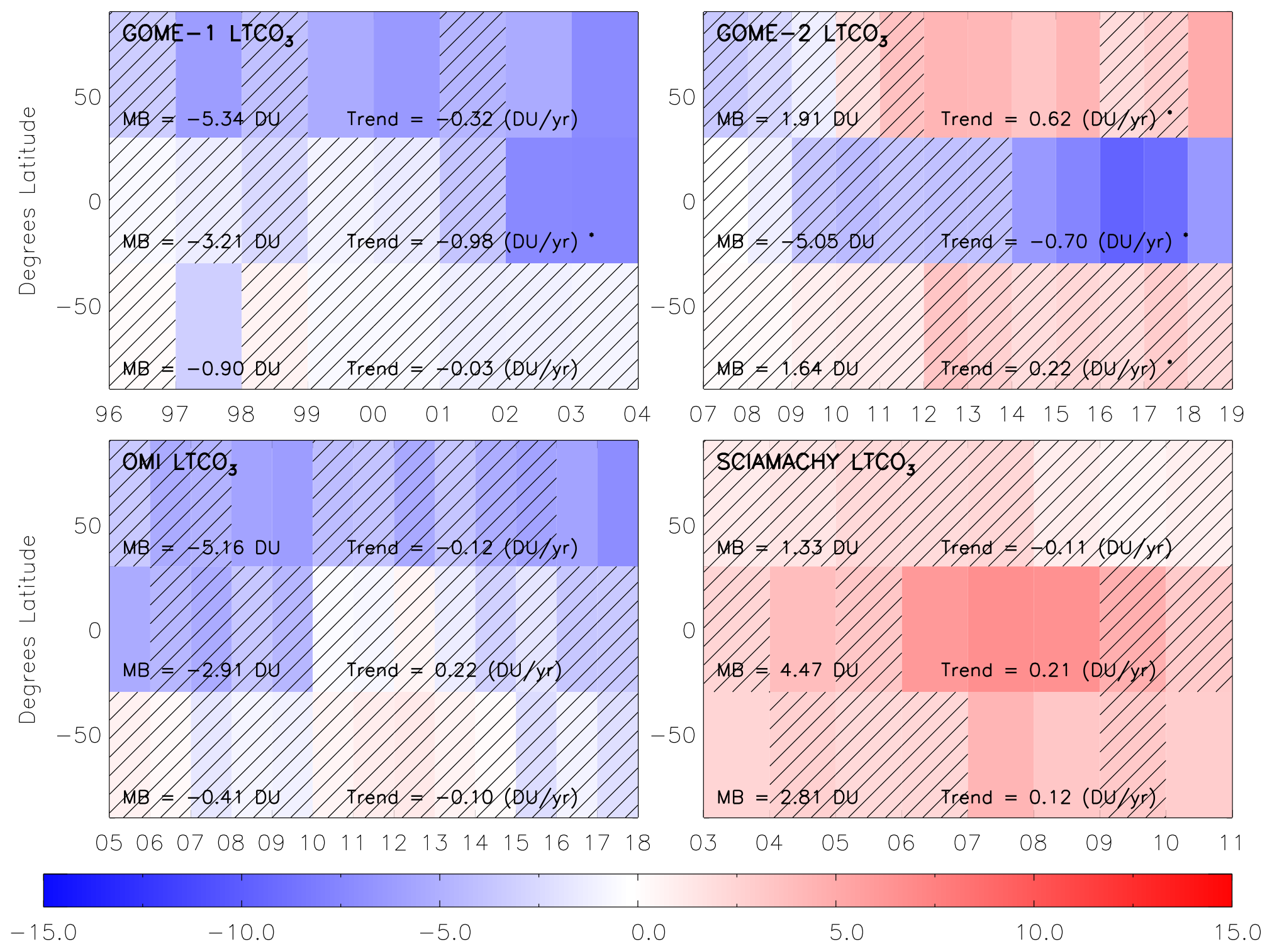
Figure 5Latitudinal–annually varying satellite sonde, with AKs applied, LTCO3 (DU) median (50th percentile) biases. Hatched regions show where the spread in the 25th and 75th percentiles intersects with 0.0. The mean bias (MB) and trend are for the full time series of each hemisphere. The ∗ for the trend term indicates that it has a p value < 0.05. The latitude bands are 90–30∘ S, 30∘ S–30∘ N and 30–90∘ N.
For GOME-2, the record MB is 1.91, −5.05 and 1.64 DU for the respective latitude bands, all of which have substantial bias trends at 0.62∗, and 0.22∗ DU yr−1. Therefore, the GOME-2 LTCO3 records from this processing run are not stable and cannot be used further in the study. SCIAMACHY has regional mean biases of 1.33, 4.47 and 2.81 DU. In the 30–90∘ N region, the bias is non-substantial. While there are substantial biases peaking at 3.0–5.0 DU in the 90–30∘ S region, neither region has a critical drift trend. The largest substantial biases are in the 30∘ S–30∘ N region (>5.0 DU) for 2006 to 2008. While the positive trend of 0.21 DU yr−1 is non-substantial, we do not use the SCIAMACHY data in later years when harmonising the LTCO3 records (Sect. 3.4). OMI has MBs of −5.16, −2.91 and −0.41 DU with only a few of the year–latitude pixels having substantial biases peaking at −6.0 to −3.0 DU in the 30–90∘ N region. The resulting bias trends are −0.12, 0.22 and −0.10 DU yr−1, which all have p values >0.05. Therefore, GOME-1, OMI and SCIAMACHY were deemed suitable LTCO3 records for use in this study.
3.4 Lower tropospheric column ozone merged record
The RAL Space products cover the full period between 1996 and 2017. Therefore, there is the opportunity to merge and harmonise these records to produce a long-term record to look at the spatiotemporal variability of LTCO3. From Fig. 5, the OMI record appears to be stable with time globally, providing a suitable data set between 2005 and 2017. The GOME-2 record appears not to be sufficiently stable across its record (2008–2018), so it is not included in subsequent analysis. The GOME-1 record covers 1996 to 2010, but given the loss of geographical coverage due to the onboard tape recorder failing in June 2003 (van Roozendael, 2012), a true global average is only available between 1996 and 2003. Figure 5 shows that GOME-1 bias with respect to the ozonesonde record is not stable in the tropics, but this is predominantly driven by instrument–ozonesonde differences in 2003. Therefore, 2003 is also dropped leaving the GOME-1 global record between 1996 and 2002. The GOME-1 tropical bias for 2002 is similar to that of 2003 (−5.0 DU), but the biases for the other latitude bands are less distinct. The regional average LTCO3 values for 2002 in Fig. 5 are also comparable to neighbouring years (e.g. 2000 and 2001). SCIAMACHY also does not have a full year of data for 2002, so we have included the GOME-1 2002 data in our analysis.
While OMI (2005–2017) and GOME-1 (1996–2002) now cover a large proportion of the global record, there is still a systematic difference between them. Different UV–Vis instruments can have inconsistencies in their retrieved products (e.g. van der A et al., 2006; Heue et al., 2016) and often require a systematic adjustment to create a harmonised record. Here, there is overlap in the raw records between 2005 and 2010 for GOME-1 and OMI. The GOME-1 record does have large missing data gaps globally, but for the mid-latitude and tropical latitude bands, there is sufficient sampling to inter-compare the two records. Therefore, for each swath, the nearest OMI retrieval is co-located to that of GOME-1 but has to be within 250 km. The local overpass times are different (i.e. GOME-1 10.30 and OMI 13.30) but within approximately 3 h, so the diurnal cycle impacts are likely to be of a secondary order and we are confident in merging the records. Based on the co-located OMI and GOME-1 data, we derived long-term latitude–month offsets which are added to GOME-1 (1996–2002) to harmonise the records. This was done using latitudinal bins of 60–30∘ S, 30∘ S–30∘ N and 30–60∘ N. Given the lack of GOME-1 data outside of 60∘ S–60∘ N due to the failure of the GOME-1 tape recorder in June 2003, there was insufficient data to derive offsets, and the high-latitude data are excluded in the following sections. Where there was good spatial coverage from GOME-1 between 2005 and 2010, once the offset had been applied, gridded OMI and GOME-1 where data existed for both, on a pixel-by-pixel basis, were averaged together.
For 2003 and 2004, we use the SCIAMACHY spatial fields to gap fill the record. Figure 5 shows that SCIAMACHY had some substantially large biases compared to the ozonesondes in 2006, 2007 and 2008 but was reasonable for other years. Therefore, we use the global distributions from SCIAMACHY for both years but scale them to expected values between 2002 and 2005. This is achieved by getting the globally weighted (based on surface area) LTCO3 average for GOME-1 (2002 with GOME-1 with the OMI offset applied) and OMI (2005) and the SCIAMACHY (2003–2004). Based on the difference between 2002 and 2005, an annual linear global scaling is applied in 2003 and 2004 for the SCIAMACHY spatial fields. Thus, we have developed a harmonised LTCO3 record between 1996 and 2017. Examples of the harmonised data for Europe and East Asia are shown in Fig. 6. Overall, there is non-linear variability in the two regional time series where red and blue show the GOME-1 and OMI LTCO3 time series, and then black shows where they have been merged (including SCIAMACHY for 2003 and 2004). For Europe (East Asia), the seasonal cycle ranges between 10.0 (13.0) and 30.0 (27.0) DU, respectively, with annual average values between 18.0 (18.0) and 22.0 (21.0) DU.
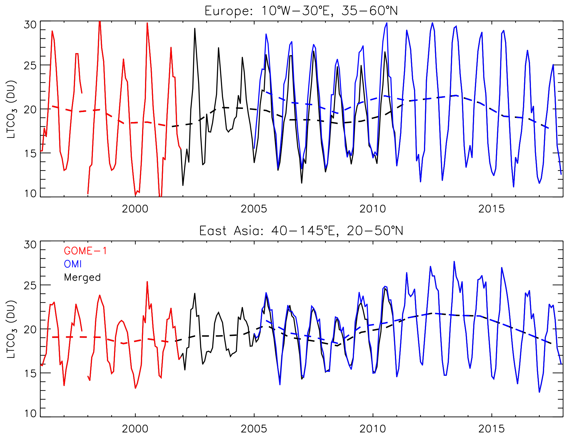
Figure 6Examples of the merged LTCO3 (DU) data set for Europe and East Asia. The GOME-1, OMI and merged time series are shown in red, blue and black, respectively. The merged record also includes globally scaled LTCO3 data from SCIAMACHY for 2003 and 2004. Dashed lines represent the annual averages, and the monthly mean time series are solid lines.
3.5 Lower tropospheric column ozone temporal variability
The harmonised RAL Space data set can now be used to investigate decadal-scale spatiotemporal variability in LTCO3. Figure 7 shows the global long-term (1996–2017) average in LTCO3 and the 5-year average anomalies for 1996–2000, 2005–2009 and 2013–2017. In the long-term average (Fig. 7a), there is clear SH to NH LTCO3 gradient with background values of 13.0–17.0 and 20–23.0 DU, respectively. There are hotspots over East Asia, the Middle East/Mediterranean and northern India of 24.0–25.0 DU. The largest SH LTCO3 values (20.0–22.0 DU) are between 30–15∘ S spanning southern Africa, the Indian Ocean and Australia. Minimum LTCO3 values (<12.0 DU) are over the Himalayas (due to topography) and the tropical oceans. As shown in Fig. 2, there is sufficient information (e.g. LTCO3 DOFS mostly >0.5) in the tropics and mid-latitudes for the instruments used to form the merged LTCO3 data. This provides confidence in this merged LTCO3 record for long-term temporal analysis. Note that the SAA has been masked out in all the panels. The 1996–2000 anomaly map (Fig. 7b) shows values to be similar (i.e. −1.0 to 1.0 DU) with respect to the 1996–2017 mean between 30 and 60∘ N. A similar relationship occurs at approximately 30∘ S. However, in tropics and NH sub-tropics (15∘ S to 30∘ N), the anomalies are more negative, ranging between approximately −3.0 and −1.0 DU. The green polygon-outlined regions show where the 1996–2000 LTCO3 average represents a substantial difference (p value < 0.05) from the long-term average. This is based on the Wilcoxon rank test (WRT), which is the nonparametric counterpart of the Student t test that relaxes the constraint on normality of the underlying distributions (Pirovanoet al., 2012). As well as this tropical band, the 60–45∘ S band shows anomalies of a similar magnitude. In the 2005–2009 anomaly map (Fig. 7c), there are widespread, though non-substantial, anomalies of −1.5.0 to 0.0 DU. There are small clusters of substantial anomalies (e.g. southern Africa at −2.0 to −1.0 DU and over the Bering Sea between 1.0 and 2.0 DU) but with limited spatial coherence. In the 2013–2017 anomaly map (Fig. 7d), there remain small LTCO3 anomalies in the northern mid-latitudes (−1.0 to 1.0 DU). A similar pattern occurs in the southern sub-tropics and mid-latitudes, though the anomalies are larger, peaking at 1.5 DU around 60–45∘ S (some have p values < 0.05). However, in the tropics and sub-tropics (15∘ S–30∘ N), there are positive anomalies of 1.0 to 2.0 DU throughout the region, peaking at 2.0–2.5 DU over Africa.
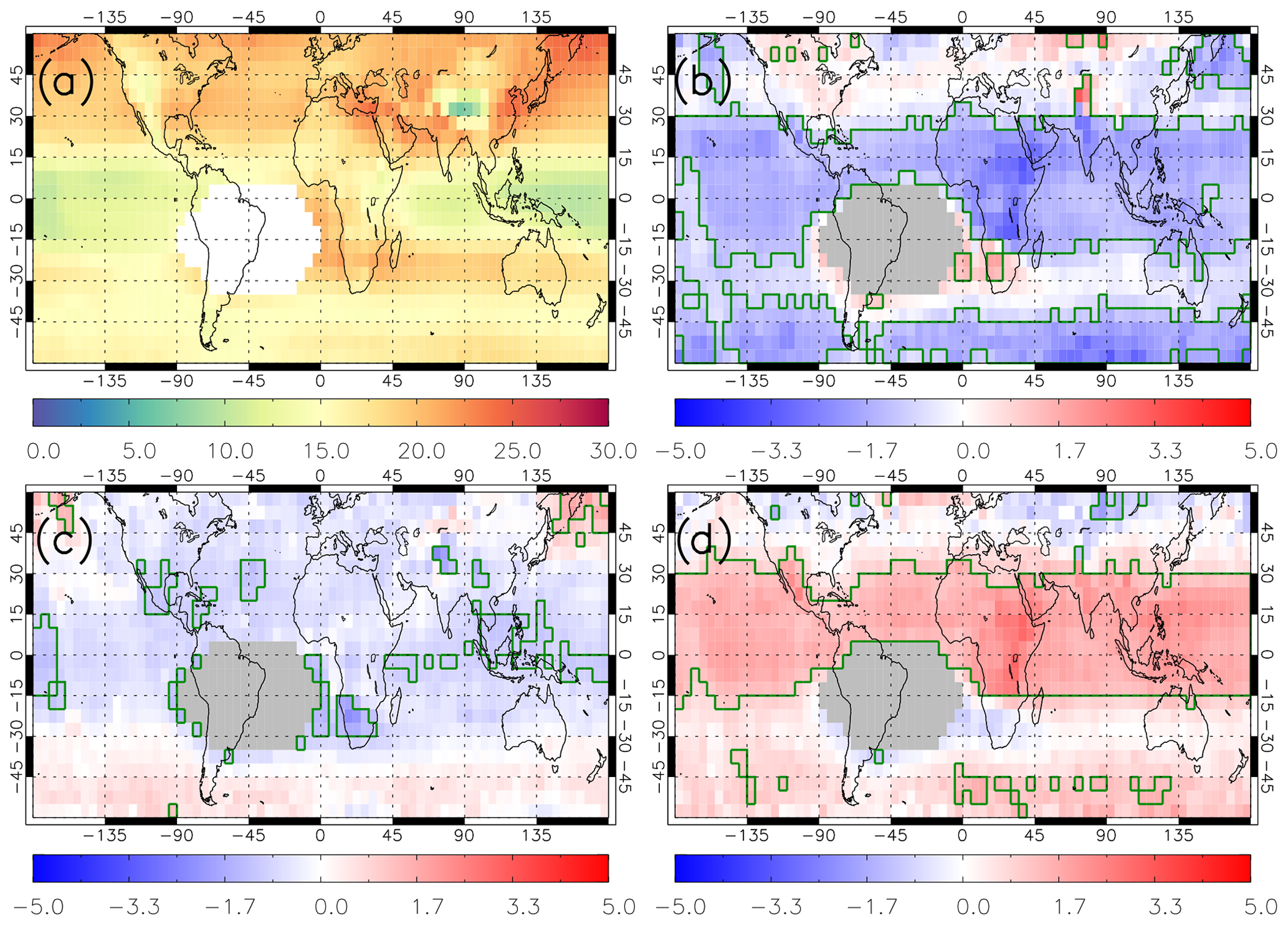
Figure 7LTCO3 (DU) merged data set from GOME-1 (1996–2002), SCIAMACHY (2003–2004) and OMI (2005–2017): (a) 1996–2017 long-term average, (b) 1996–2000 average anomaly, (c) 2005–2009 average anomaly and (d) 2013–2017 average anomaly. Anomalies are relative to the long-term average (a). Green polygon-outlined regions show substantial anomalies (95 % confidence level and where the absolute anomaly >1.0 DU) from the long-term average using the Wilcoxon rank test. White/grey pixels are where the South Atlantic Anomaly influence on retrieved LTCO3 has been masked out.
Overall, these anomalies suggest there has been limited change in LTCO3, between 1996 and 2017, in the NH mid-latitudes (e.g. as can be seen for Europe and East Asia in Fig. 6). Unfortunately, the SAA masks any useful information on LTCO3 over South America, but generally there has been a moderate LTCO3 increase in the SH mid-latitudes. The largest and most substantial changes have been in the tropics and sub-tropics (i.e. 15∘ S to 30∘ N) switching from sizeable negative anomalies (−2.0 to −1.0 DU) in the 1996–2000 LTCO3 average to positive anomalies (1.0–2.0 DU) in the 2013–2017 LTCO3. Figure 8 shows the difference between the 2013–2017 and 1996–2000 averages. Over the tropics/sub-tropics (15∘ S–30∘ N), the largest increases (p values <0.05) of 3.0 to 5.0 DU peak in Africa, India and South-East Asia (>5.0 DU), thus, showing a large-scale increase in tropical LTCO3 between 1996 and 2017. In the NH mid-latitudes, the absolute LTCO3 differences are relatively small (−1.0 to −1.5 DU), but they are consistent, though some negative differences (generally −2.0 and −1.0 DU) are over North America and Russia. In the SH mid-latitudes, there has been a moderate increase in LTCO3 of 2.0–3.5 DU. However, southern Africa shows more localised decreases of up to 3.0 DU and non-substantial differences at 30∘ S across the Indian Ocean. The ozonesondes are consistent with satellite 1996–2000 and 2013–2017 average LTCO3 differences. In the tropics, the majority of ozonesonde sites show increases between these two periods ranging between 0.5 and 5.0 DU. Over Europe (i.e. northern mid-latitudes), the ozonesonde LTCO3 differences range between −0.5 and 0.5 DU, suggesting limited LTCO3 change over time.
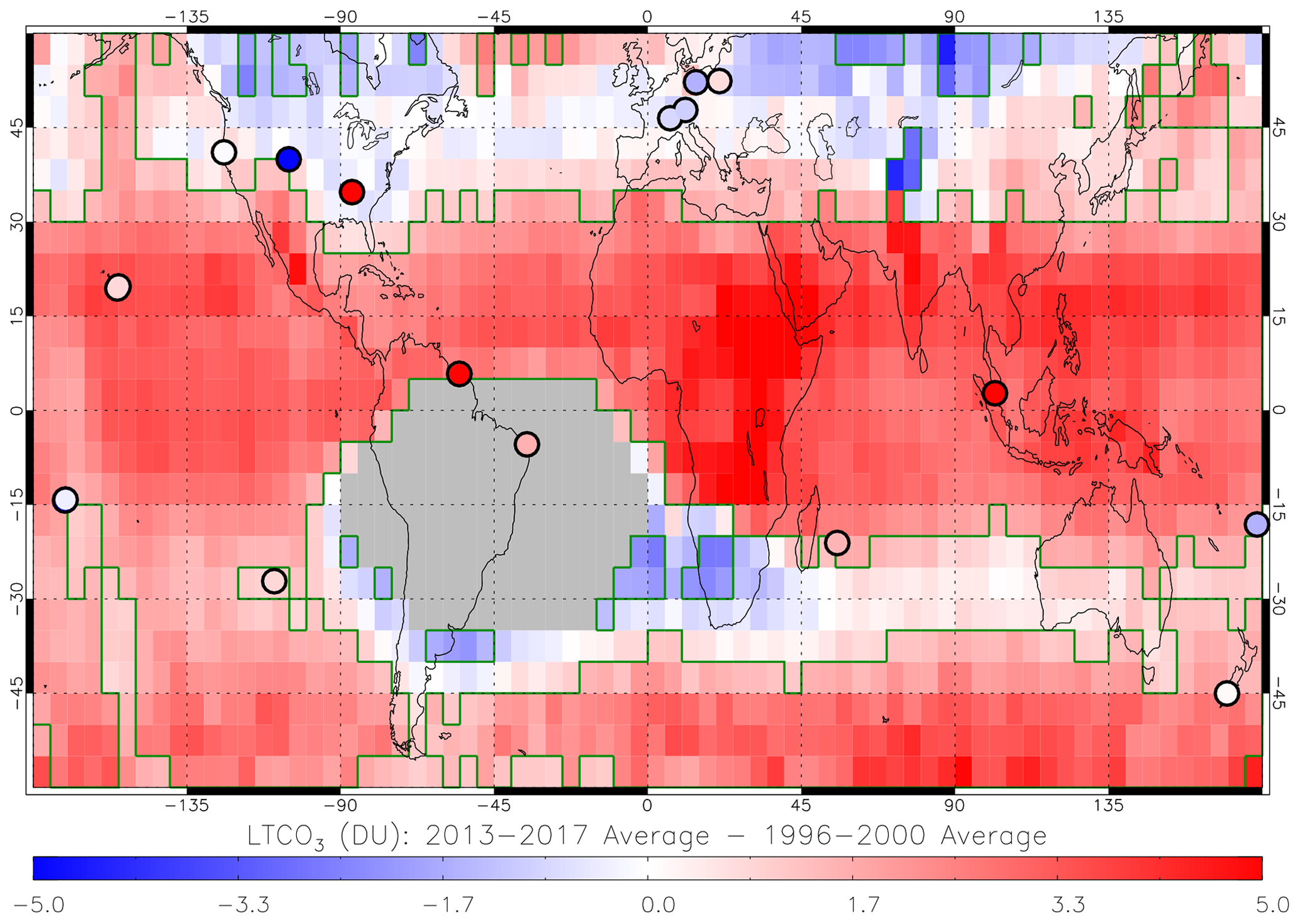
Figure 8LTCO3 (DU) merged data set from GOME-1 (1996–2002), SCIAMACHY (2003–2004) and OMI (2005–2017) where the difference between the 2013–2017 average and 1996–2000 average is shown. Green polygon-outlined regions show substantial differences (95 % confidence level and where the absolute difference >1.0 DU) using the Wilcoxon rank test. Grey pixels are where the South Atlantic Anomaly influence on retrieved LTCO3 has been masked out. Circles show differences in ozonesonde LTCO3 (DU) over the same time periods as the merged satellite record.
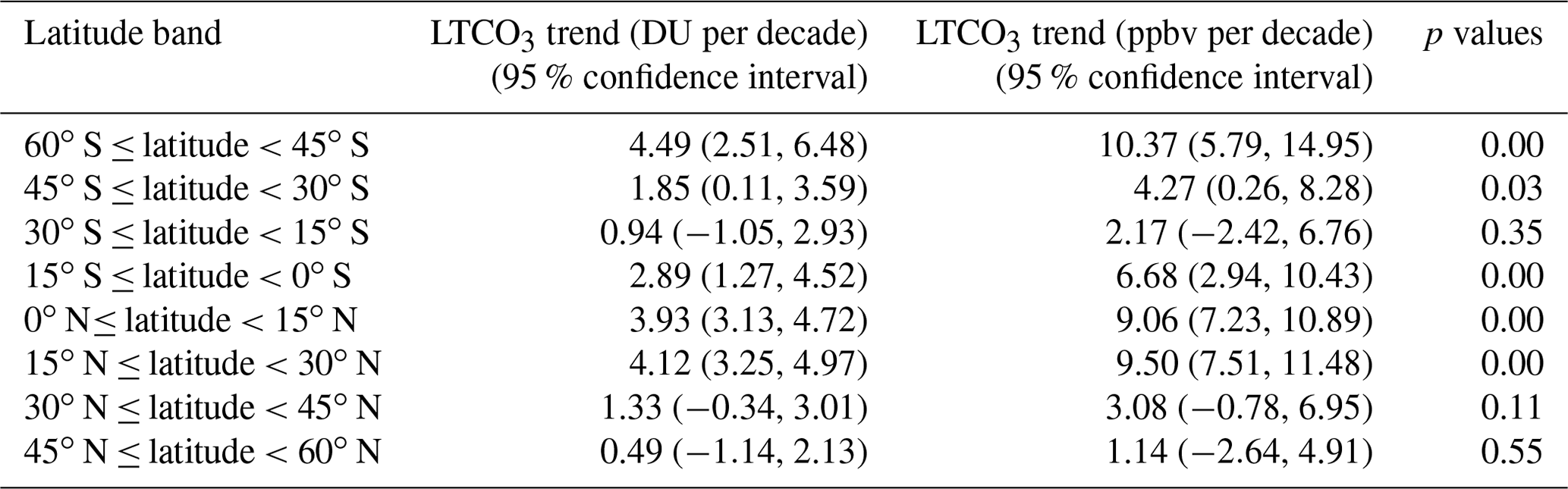
Table 2LTCO3 trends (DU per decade and ppbv per decade) for latitude bands (15∘ bins) between 60∘ S and 60∘ N. The 95 % confidence intervals of the trends are shown in brackets. The trend p values are also shown.
3.6 Long-term LTCO3 trends
In line with TOAR-II, we have added additional metrics on the temporal change in LTCO3 over the merged instrument record. Here, we have calculated the linear trends in LTCO3 in 15∘ latitude bins between 60∘ S–60∘ N along with the 95 % confident range and associated p values (see Table 2). In the tropical latitudes (15∘ S–30∘ N), all the linear trends show substantial increasing trends (2.89–4.12 DU per decade) between 1996 and 2017, all with p values tending to 0.0. This is consistent with the LTCO3 positive differences (3.0–5.0 DU) between the 1996–2000 and 2013–2017 averages (Fig. 8). In the northern mid-latitudes (30–60∘ N), there are smaller positive trends (1.33 and 0.49 DU per decade), but the 95 % confidence values intersect with 0.0 and have larger p values. Again, this is consistent with the near-zero differences between the 1996–2000 and 2013–2017 averages (Fig. 8). In the southern mid-latitudes (30–60∘ S), the trends are substantially positive (1.85 and 4.49 DU per decade) with near-zero p values. Again, this is consistent with the substantial differences (2.0–4.0 DU) between the 1996–2000 and 2013–2017 averages. The 15–30∘ S trend is small at 0.94 DU per decade with a moderate p value of 0.35, indicating this not to be a substantial trend.
Multiple studies have used satellite records to investigate change in TCO3 in recent decades. Gaudel et al. (2018) used a range of UV–Vis and IR TCO3 products between 2005 and 2016. The UV–Vis sounders generally show substantial positive trends (0.1–0.8 DU yr−1) in the tropics/sub-tropics and a mixed response in the mid-latitudes. The IR instruments typically showed significant decreasing trends (−0.5 to −0.2 DU yr−1) in background regions and isolated regions of substantial TCO3 enhancements. Ziemke et al. (2019) used a long-term merged record of TCO3 from the Total Ozone Mapping Spectrometer (TOMS) and Ozone Monitoring Instrument/Microwave Limb Sounder (OMI-MLS) between 1979 and 2016. Over this period, they found significant increases of TCO3 of 1.5 to 6.5 DU, especially over India and East Asia. Heue et al. (2016) used a long-term tropical TCO3 record (GOME, SCIAMACHY, OMI, GOME-2A and GOME-2B) finding significant increases (0.5–2.0 DU per decade) over central Africa and the South Atlantic. However, the study by Wespes et al. (2018) from IASI (an IR sounder) indicated that TCO3 decreased between 2008 and 2017 by −0.5 to −0.1 DU yr−1. Gaudel et al. (2018) reported similar TCO3 tendencies using two IASI products (IASI-FORLI and IASI-SOFRID). However, Boynard et al. (2018) and Wespes et al. (2018) report a step change in 2010 in the IASI-FORLI O3 data which could influence observed long-term trends. Therefore, studies using IR products available to TOAR-I and Wespes (2018) are no longer considered reliable.
In this study, for the first time we analysed long-term changes in LTCO3 using a merged satellite UV–Vis sounder record. Overall, we found that LTCO3 was lower (by 1.0–3.0) in the tropics between 1996 and 2000 in comparison to the long-term average (i.e. 1996–2017). Similar LTCO3 values exist between the 2005–2009 and long-term averages, while the 2013–2017 average shows substantially larger tropical values (1.0–2.5 DU) than the long-term average. Therefore, this tropical increase (3.0–5.0 DU) in LTCO3 between 1996 and 2017 is consistent with other reported increases in TCO3. A similar consistency is found in the NH mid-latitudes, with minimal changes in LTCO3 observed here and in trends in TCO3 reported in Gaudel et al. (2018) and Ziemke et al. (2019). Sizable LTCO3 increases in the SH mid-latitudes are also consistent with Gaudel et al. (2018) and Ziemke et al. (2019), though they differ from IASI-retrieved TCO3 trends as reported by Wespes et al. (2018). Overall, the long-term changes in LTCO3 reported here and the literature TCO3 trends from satellite UV products are comparable in regard to latitude dependence and direction. It therefore seems that the positive tendencies in TCO3 reported in the literature from UV soundings over the satellite era are associated with, and could be driven by, changes occurring in LTCO3.
For future work, a detailed study is required to disentangle the reported TCO3 and LTCO3 trends reported by UV–Vis and IR sounders, which would benefit from satellite level-2 data produced from level-1 data sets which are more uniform over time along with other improvements. This can potentially be done also by using a 3D atmospheric chemistry model (ACM) to investigate the changes in lower and upper tropospheric ozone and application of the satellite AKs (i.e. the vertical sensitivity of the different satellite products) to the model from the different sounders to establish how satellite vertical sensitivity potentially changes the simulated TO3 tendency of the model. An ACM would also be a useful tool to help diagnose the importance of LTCO3 contributions to the TCO3 tendencies and which processes might be driving any spatiotemporal changes (e.g. surface emissions, atmospheric chemistry/surface deposition, stratospheric–tropospheric O3 exchanges). Finally, together with improved, extended reprocessed versions of the data sets used in this study, the launch of the Sentinel 5 Precursor (S5P) satellite (in October 2017) can be used to extend the merged data record of LTCO3, along with new polar-orbiting platforms such as Sentinel-5 and IASI-NG instruments on future EUMETSAT MetOp-Second Generation satellites.
The RAL Space satellite data is available via the NERC Centre for Environmental Data Analysis (CEDA) Jasmin platform (http://www.ceda.ac.uk/, last access: 2 January 2023) and the harmonised LTCO3 data record (from GOME-1, SCIAMACHY and OMI) for 1996–2017 has been uploaded to Zenodo (https://doi.org/10.5281/zenodo.10184945), which is publicly available.
RJP, MPC and BJK conceptualised and planned the research study. RJP and MAP analysed the satellite data provided by RAL Space (BJK, RS, BGL) with support from BJK, RS and BGL. MPC, SSD and CR provided scientific advice, while WF and RR provided technical support. RJP prepared the manuscript with contributions from all co-authors.
The contact author has declared that none of the authors has any competing interests.
Publisher’s note: Copernicus Publications remains neutral with regard to jurisdictional claims made in the text, published maps, institutional affiliations, or any other geographical representation in this paper. While Copernicus Publications makes every effort to include appropriate place names, the final responsibility lies with the authors.
This article is part of the special issue “Tropospheric Ozone Assessment Report Phase II (TOAR-II) Community Special Issue (ACP/AMT/BG/GMD inter-journal SI)”. It is a result of the Tropospheric Ozone Assessment Report, Phase II (TOAR-II, 2020–2024).
This work was funded by the UK Natural Environment Research Council (NERC) by providing funding for the National Centre for Earth Observation (NCEO, award reference NE/R016518/1) and funding from the European Space Agency (ESA) Climate Change Initiative (CCI) post-doctoral fellowship scheme (contract number 4000137140). Anna Maria Trofaier (ESA Climate Office) provided support and advice throughout the fellowship.
This research has been supported by the National Centre for Earth Observation (grant no. NE/R016518/1) and the European Space Agency (grant no. 4000137140).
This paper was edited by Jayanarayanan Kuttippurath and reviewed by two anonymous referees.
Boersma, K. F., Eskes, H. J., Dirksen, R. J., van der A, R. J., Veefkind, J. P., Stammes, P., Huijnen, V., Kleipool, Q. L., Sneep, M., Claas, J., Leitão, J., Richter, A., Zhou, Y., and Brunner, D.: An improved tropospheric NO2 column retrieval algorithm for the Ozone Monitoring Instrument, Atmos. Meas. Tech., 4, 1905–1928, https://doi.org/10.5194/amt-4-1905-2011, 2011.
Copernicus: Product Quality Assessment Report (PQAR) Ozone products – Version 2.0b, Issued by BIRA-IASB/Jean-Christopher Lambert, Ref: C3S_D312b_Lot2.2.1.2_202105_PQAR_O3_v2.0b, 2021.
ESA: Climate Change Initiative, http://cci.esa.int/ozone (last access: 2 May 2023), 2019.
Eskes, H. J. and Boersma, K. F.: Averaging kernels for DOAS total-column satellite retrievals, Atmos. Chem. Phys., 3, 1285–1291, https://doi.org/10.5194/acp-3-1285-2003, 2003.
Forster, P., Storelvmo, T., Armour, K., Collins, W., Dufresne, J.-L., Frame, D., Lunt, D. J., Mauritsen, T., Palmer, M. D., Watanabe, M., Wild, M., and Zhang, H.: The Earth’s Energy Budget, Climate Feedbacks, and Climate Sensitivity, in: Climate Change 2021: The Physical Science Basis, Contribution of Working Group I to the Sixth Assessment Report of the Intergovernmental Panel on Climate Change, edited by: Masson-Delmotte, V., Zhai, P., Pirani, A., Connors, S. L., Péan, C., Berger, S., Caud, N., Chen, Y., Goldfarb, L., Gomis, M. I., Huang, M., Leitzell, K., Lonnoy, E., Matthews, J. B. R.,Maycock, T. K., Waterfield, T., Yelekçi, O., Yu, R., and Zhou, B., Cambridge University Press, Cambridge, United Kingdom and New York, NY, USA, 923–1054, doi:10.1017/9781009157896.009, 2021.
Gaudel, A., Cooper, O. R., Ancellet, G., Barret, B., Boynard, A., Burrows, J. P., Clerbaux, C., Coheur, P. F., Cuesta, J., Cuevas, E., Doniki, S., Dufour, G., Ebojie, F., Foret, G., Garia, O., Granados-Munoz, M. J., Hannigan, J. W., Hase, F., Hassler, B., Huang, G., Hurtmans, D., Jaffe, D., Jones, N., Kalabokas, P., Kerridge, B., Kulwaik, S., Latter, B., Leblanc, T., Le Flochmoen, E., Lin, W., Liu, J., Liu, X., Mahieu, E., McClure-Begley, A., Neu, J. L., Osman, M., Palm, M., Petetin, H., Petropavlovskikh, I., Querel, R., Rahpoe, N., Rozanov, A., Schultz, M. G., Schwab, J., Siddans, R., Smale, D., Steinbacher, M., Tanimoto, H., Tarasick, D. W., Thouret, V., Thompson, A. M., Trickl, T., Weatherhead, E., Wespes, C., Worden, H. M., Vigouroux, C., Xu, X., Zeng, G., and Ziemke, J.: Tropospheric Ozone Assessment Report: Present day distribution and trends of tropospheric ozone relevant to climate and global atmospheric chemistry model evaluation, Elementa, 6, 1–58, https://doi.org/10.1525/elementa.291, 2018.
Gauss, M., Myhre, G., Isaksen, I. S. A., Grewe, V., Pitari, G., Wild, O., Collins, W. J., Dentener, F. J., Ellingsen, K., Gohar, L. K., Hauglustaine, D. A., Iachetti, D., Lamarque, F., Mancini, E., Mickley, L. J., Prather, M. J., Pyle, J. A., Sanderson, M. G., Shine, K. P., Stevenson, D. S., Sudo, K., Szopa, S., and Zeng, G.: Radiative forcing since preindustrial times due to ozone change in the troposphere and the lower stratosphere, Atmos. Chem. Phys., 6, 575–599, https://doi.org/10.5194/acp-6-575-2006, 2006.
Heue, K.-P., Coldewey-Egbers, M., Delcloo, A., Lerot, C., Loyola, D., Valks, P., and van Roozendael, M.: Trends of tropical tropospheric ozone from 20 years of European satellite measurements and perspectives for the Sentinel-5 Precursor, Atmos. Meas. Tech., 9, 5037–5051, https://doi.org/10.5194/amt-9-5037-2016, 2016.
Hubert, D., Lambert, J.-C., Verhoelst, T., Granville, J., Keppens, A., Baray, J.-L., Bourassa, A. E., Cortesi, U., Degenstein, D. A., Froidevaux, L., Godin-Beekmann, S., Hoppel, K. W., Johnson, B. J., Kyrölä, E., Leblanc, T., Lichtenberg, G., Marchand, M., McElroy, C. T., Murtagh, D., Nakane, H., Portafaix, T., Querel, R., Russell III, J. M., Salvador, J., Smit, H. G. J., Stebel, K., Steinbrecht, W., Strawbridge, K. B., Stübi, R., Swart, D. P. J., Taha, G., Tarasick, D. W., Thompson, A. M., Urban, J., van Gijsel, J. A. E., Van Malderen, R., von der Gathen, P., Walker, K. A., Wolfram, E., and Zawodny, J. M.: Ground-based assessment of the bias and long-term stability of 14 limb and occultation ozone profile data records, Atmos. Meas. Tech., 9, 2497–2534, https://doi.org/10.5194/amt-9-2497-2016, 2016.
Keppens, A., Lambert, J.-C., Granville, J., Hubert, D., Verhoelst, T., Compernolle, S., Latter, B., Kerridge, B., Siddans, R., Boynard, A., Hadji-Lazaro, J., Clerbaux, C., Wespes, C., Hurtmans, D. R., Coheur, P.-F., van Peet, J. C. A., van der A, R. J., Garane, K., Koukouli, M. E., Balis, D. S., Delcloo, A., Kivi, R., Stübi, R., Godin-Beekmann, S., Van Roozendael, M., and Zehner, C.: Quality assessment of the Ozone_cci Climate Research Data Package (release 2017) – Part 2: Ground-based validation of nadir ozone profile data products, Atmos. Meas. Tech., 11, 3769–3800, https://doi.org/10.5194/amt-11-3769-2018, 2018.
Lamarque, J.-F., Bond, T. C., Eyring, V., Granier, C., Heil, A., Klimont, Z., Lee, D., Liousse, C., Mieville, A., Owen, B., Schultz, M. G., Shindell, D., Smith, S. J., Stehfest, E., Van Aardenne, J., Cooper, O. R., Kainuma, M., Mahowald, N., McConnell, J. R., Naik, V., Riahi, K., and van Vuuren, D. P.: Historical (1850–2000) gridded anthropogenic and biomass burning emissions of reactive gases and aerosols: methodology and application, Atmos. Chem. Phys., 10, 7017–7039, https://doi.org/10.5194/acp-10-7017-2010, 2010.
Miles, G. M., Siddans, R., Kerridge, B. J., Latter, B. G., and Richards, N. A. D.: Tropospheric ozone and ozone profiles retrieved from GOME-2 and their validation, Atmos. Meas. Tech., 8, 385–398, https://doi.org/10.5194/amt-8-385-2015, 2015.
Myhre, G., Shindell, D., Breon, F.-M., Collins, W., Fuglestvedt, J., Huang, J., Koch, D., Lamarque, J.-F., Lee, D., Mendoza, B., Nakajima, T., Zhang, H., Aamaas, B., Boucher, O., Dalsoren, S. B., Daniel, J. S., Forster, P., Granier, C., Haigh, J., Hodnebrog, O., Kaplan, J. O., Marston, G., Nielsen, C.J., O'Neil, B. C., Peters, G. P., Pongratz, J., Prather, M., Ramaswamy, V., Roth, R., Rotstayn, L., Smith, S. J., Stevenson, D., Vernier, J.-P., Wild, O., and Young.: Anthropogenic and Natural Radiative Forcing, in: Climate Change 2013: The Physical Science Basis. Contribution of Working Group I to the Fifth Assessment Report of the Intergovernmental Panel on Climate Change Cambridge University Press, Cambridge, United Kingdom and New York, NY, USA, 659–740, 2013.
Pope, R. J., Arnold, S. R., Chipperfield, M. P., Latter, B. G., Siddans, R., and Kerridge, B. J.: Widespread changes in UK air quality observed from space, Atmos. Sci. Lett., 19, e817, https://doi.org/10.1002/asl.817, 2018.
Pope, R. J., Arnold, S. R., Chipperfield, M. P., Reddington, C. L. S., Butt, E. W., Keslake, T. D., Feng, W., Latter, B. G., Kerridge, B. J., Siddans, R., Rizzo, L., Artazo, P., Sadiq, M., and Tai, A. P. K.: Substantial Increases in Eastern Amazon and Cerrado Biomass Burning-Sourced Tropospheric Ozone, Geophys. Res. Lett., 47, e2019GL084143, https://doi.org/10.1029/2019GL084143, 2020.
Pope, R.: Investigation of spatial and temporal variability in lower tropospheric ozone from RAL Space UV-Vis satellite products, Zenodo [data set], https://doi.org/10.5281/zenodo.10184945, 2023.
Pirovano, G., Balzarini, A., Bessagnet, B., Emery, C., Kallos, G., Meleux, F., Mitskaou, C., Nopmongcol, U., Riva, G. M., and Yarwood, G.: Investigating impacts of chemistry and transport model formulation on model performance at European scale, Atmos. Environ., 59, 93–109, https://doi.org/10.1016/j.atmosenv.2011.12.052, 2012.
Richards, N. A. D., Arnold, S. R., Chipperfield, M. P., Miles, G., Rap, A., Siddans, R., Monks, S. A., and Hollaway, M. J.: The Mediterranean summertime ozone maximum: global emission sensitivities and radiative impacts, Atmos. Chem. Phys., 13, 2331–2345, https://doi.org/10.5194/acp-13-2331-2013, 2013.
Rodgers, C. D.: Inverse methods for atmospheric sounding: Theory and practice, New Jersey, USA, World Scientific Publishing, ISBN 978-981-02-2740-1, 2000.
Russo, M. R., Kerridge, B. J., Abraham, N. L., Keeble, J., Latter, B. G., Siddans, R., Weber, J., Griffiths, P. T., Pyle, J. A., and Archibald, A. T.: Seasonal, interannual and decadal variability of tropospheric ozone in the North Atlantic: comparison of UM-UKCA and remote sensing observations for 2005–2018, Atmos. Chem. Phys., 23, 6169–6196, https://doi.org/10.5194/acp-23-6169-2023, 2023.
Shah, S., Tuinder, O. N. E., van Peet, J. C. A., de Laat, A. T. J., and Stammes, P.: Evaluation of SCIAMACHY Level-1 data versions using nadir ozone profile retrievals in the period 2003–2011, Atmos. Meas. Tech., 11, 2345–2360, https://doi.org/10.5194/amt-11-2345-2018, 2018.
Sitch, S., Cox, P. M., Collins, W. J., and Huntingford, C.: Indirect radiative forcing of climate change through ozone effects on the land carbon sink, Nature, 448, 791–795, https://doi.org/10.1038/nature06059, 2007.
Stauffer, R. M., Thompson, A. M., Kollonige, D. E., Witte, J. C., Tarasick, D. W., Davies, J., Vomel, H., Morris, G. A., Van Malderen, R., Johnson, B. J., Querel, R. R., Selkirk, H. B., Stubi, R., and Smit, H. G. J.: A post-2013 Dropoff in Total Ozone at a Third of Global Ozonesonde Stations: Electrochemical Concentration Cell Instrument Artefacts?, Geophys. Res. Lett., 47, e2019GL086791, https://doi.org/10.1029/2019GL086791, 2020.
Torres, O., Bhartia, P. K., Jethva, H., and Ahn, C.: Impact of the ozone monitoring instrument row anomaly on the long-term record of aerosol products, Atmos. Meas. Tech., 11, 2701–2715, https://doi.org/10.5194/amt-11-2701-2018, 2018.
van der A, R. J., Peters, D. H. M. U., Eskes, H., Boersma, K. F., Van Roozendael, M., De Smedt, I., and Kelder, H. M.: Detection of the trend and seasonal variation in tropospheric NO2 over China, J. Geophys. Res., 11, D12317, https://doi.org/10.1029/2005JD006594, 2006.
Van Roozendael, M., Spurr, R., Loyola, D., Lerot, C., Balis, D., Lambert, J.-C., Zimmer, W., van Gent, J., van Geffen, J., Kouklouli, M., Granville, J., Doicu, A., Fayt, C., and Zehner, C.: Sixteen years of GOME/ERS-2 total ozone data: The new direct-fitting GOME Data Processor (GDP) version 5 – Algorithm description, J. Geophys. Res., 117, D03305, doi:10.1029/2011JD016471, 2012.
Verstraeten, W. W., Neu, J. L., Williams, J. E., Bowman, K. W., Worden, J. R., and Boersma, K. F.: Rapid increase in tropospheric ozone production and export from China, Nat. Geosci., 8, 690–695, https://doi.org/10.1038/NGEO2493, 2015.
Wespes, C., Hurtmans, D., Clerbaux, C., Boynard, A., and Coheur, P.-F.: Decrease in tropospheric O3 levels in the Northern Hemisphere observed by IASI, Atmos. Chem. Phys., 18, 6867–6885, https://doi.org/10.5194/acp-18-6867-2018, 2018.
Young, P. J., Archibald, A. T., Bowman, K. W., Lamarque, J.-F., Naik, V., Stevenson, D. S., Tilmes, S., Voulgarakis, A., Wild, O., Bergmann, D., Cameron-Smith, P., Cionni, I., Collins, W. J., Dalsøren, S. B., Doherty, R. M., Eyring, V., Faluvegi, G., Horowitz, L. W., Josse, B., Lee, Y. H., MacKenzie, I. A., Nagashima, T., Plummer, D. A., Righi, M., Rumbold, S. T., Skeie, R. B., Shindell, D. T., Strode, S. A., Sudo, K., Szopa, S., and Zeng, G.: Pre-industrial to end 21st century projections of tropospheric ozone from the Atmospheric Chemistry and Climate Model Intercomparison Project (ACCMIP), Atmos. Chem. Phys., 13, 2063–2090, https://doi.org/10.5194/acp-13-2063-2013, 2013.
Ziemke, J. R., Chandra, S., Dincan, B. N., Froidevaux, L., Bhartia, P. K., Levelt, P. F., and Walters, J. W.: Tropospheric ozone determined from Aura OMI and MLS: Evaluation of measurements and comparison with the Global Modelling Initiative's Chemical Transport Model, J. Geophys. Res., 111, D19303, https://doi.org/10.1029/2006JD007089, 2006.
Ziemke, J. R., Chandra, S., Labow, G. J., Bhartia, P. K., Froidevaux, L., and Witte, J. C.: A global climatology of tropospheric and stratospheric ozone derived from Aura OMI and MLS measurements, Atmos. Chem. Phys., 11, 9237–9251, https://doi.org/10.5194/acp-11-9237-2011, 2011.
Ziemke, J. R., Oman, L. D., Strode, S. A., Douglass, A. R., Olsen, M. A., McPeters, R. D., Bhartia, P. K., Froidevaux, L., Labow, G. J., Witte, J. C., Thompson, A. M., Haffner, D. P., Kramarova, N. A., Frith, S. M., Huang, L.-K., Jaross, G. R., Seftor, C. J., Deland, M. T., and Taylor, S. L.: Trends in global tropospheric ozone inferred from a composite record of TOMS/OMI/MLS/OMPS satellite measurements and the MERRA-2 GMI simulation, Atmos. Chem. Phys., 19, 3257–3269, https://doi.org/10.5194/acp-19-3257-2019, 2019.
The requested paper has a corresponding corrigendum published. Please read the corrigendum first before downloading the article.
- Article
(13348 KB) - Full-text XML