Revisiting the question “Why is the sky blue?”

The common answer to the question “Why is the sky blue?” is usually Rayleigh scattering. In 1953 Edward Hulburt demonstrated that Rayleigh scattering accounts for $\mathrm{1}/\mathrm{3}$ and ozone absorption for $\mathrm{2}/\mathrm{3}$ of the blue colour of the zenith sky at sunset. In this study, an approach to quantify the contribution of ozone to the blue colour of the sky for different viewing geometries is implemented using the radiative transfer model SCIATRAN and the CIE (International Commission on Illumination) XYZ 1931 colour system. The influence of ozone on the blue colour of the sky is calculated for solar zenith angles of 10–90^∘ and a wide range of viewing geometries. For small solar zenith angles, the influence of ozone on the blue colour of the sky is minor, as expected. However, the effect of ozone increases with increasing solar zenith angle. The calculations for the Sun at the horizon confirm Hulburt's estimation with remarkably good agreement. More stratospheric aerosols reduce the ozone contribution at and near the zenith for the Sun at the horizon. The exact contribution of ozone depends strongly on the assumed total ozone column. The calculations also show that the contribution of ozone increases with increasing viewing zenith angle and total ozone column. Variations in surface albedo as well as full treatment of polarised radiative transfer were found to have only minor effects on the contribution of ozone to the blue colour of the sky. Furthermore, with an observer at 10 km altitude an increase in the ozone influence can be seen.

1 Introduction

The blue colour of the cloud-free sky is one of the most obvious and self-evident features of our natural environment and has puzzled humans for thousands of years. The blue colour of the sky is nowadays usually explained by Rayleigh scattering, an explanation that is, however, not entirely correct. In his 1953 publication entitled “Explanation of the Brightness and Color of the Sky, Particularly the Twilight Sky”, Edward Olson Hulburt (1890–1982) demonstrated that for specific illumination and viewing conditions, Rayleigh scattering plays only a second-order role for the blue colour of the sky. Based on simplified radiative transfer simulations and single-scattering approximation, Hulburt (1953) concluded that for a solar zenith angle (SZA) of 90^∘ only $\mathrm{1}/\mathrm{3}$ of the blue colour of the sky of the zenith is caused by Rayleigh scattering and $\mathrm{2}/\mathrm{3}$ by absorption of solar radiation in the Chappuis bands of O₃. Interestingly, Hulburt (1953) did not explain how these contributions of Rayleigh scattering and O₃ absorption were determined. However, it can be assumed that the estimation is based on the spectra calculated by Hulburt (Hulburt, 1953, Fig. 5 therein). In the present paper we define a metric that allows determination of the effect of O₃ absorption on the blue sky colour in a quantitative way.

In the following we briefly review different explanations for the blue colour of the sky that were suggested in the past. According to See (1904), Leonardo da Vinci suggested that the blue colour of the sky is caused by mixing sunlight with the black colour of space. Newton was of the opinion that the blue of the sky was caused by small water particles that “reflect” blue light (Newton, 1730). Their size was assumed to be so small as to leave the atmosphere transparent. Newton expected larger particles to reflect different colours. Newton's theory was generally accepted well into the 19th century. An important realisation of the first half of the 19th century was that of the polarisation of sunlight scattered in the atmosphere by Francois Arago in 1809 (Hoeppe, 2007). Of essential importance for the understanding of the blue sky colour were the laboratory experiments by John Tyndall, e.g. described in Tyndall (1869). Tyndall produced tiny particles of many different compositions in a glass cylinder and observed the colour and the polarisation of scattered radiation. He found, “In all cases, and with all substances, the cloud formed at the commencement, when the precipitated particles are sufficiently fine, is blue”. (Tyndall, 1869). Furthermore, he found that these blue clouds in all cases completely polarised the scattered radiation with the direction of polarisation and the propagation direction of the incident beam forming a right angle. In 1871 John William Strutt (Baron Rayleigh III from 1873) provided a theory for both the polarisation and the spectral dependence of radiation scattered by particles which are small compared to the wavelength (Strutt, 1871). Regarding the spectral dependence, he first gave a derivation of the famous λ⁻⁴ law solely based on dimensional analysis, followed by an analytical derivation. Strutt (1871) also provided a comparison of his theoretical considerations with observations of the spectral dependence of the intensity of zenith scattered sunlight, showing good agreement. However, the nature of the small particles causing the blue colour of the sky and its polarisation was not yet established. Only in 1899 did Lord Rayleigh III demonstrate that scattering by air molecules is sufficient to explain the observed effects (Lord Rayleigh, 1899).

Adams et al. (1974) investigated the influence of ozone and aerosols on the brightness and colour of the twilight sky, using five different models of the atmosphere, such as a pure molecular scattering atmosphere, a molecular atmosphere with ozone and three models with varying aerosol concentrations. For this purpose, the authors calculated the radiance and colour of the twilight sky for solar zenith angles of 90–96^∘ assuming single scattering (more information in Sect. 3). Adams et al. (1974), as well as Gadsden (1957), Dave and Mateer (1968), and Lee et al. (2011), for example, focused on twilight conditions, i.e. solar zenith angles greater than 90^∘, and the zenith sky observations. The investigations in the present paper cover solar zenith angles of 10–90^∘ with a wide range of viewing geometries.

The paper is structured as follows. In Sect. 2 the radiative transfer model SCIATRAN, the colour representation in the International Commission on Illumination (CIE) chromaticity diagram and the method for determining the ozone contribution to the blue colour of the sky are introduced. Section 3 presents the main results with discussion, and the conclusions are given at the end (Sect. 4).

2 Methodology

2.1 Radiative transfer simulations with SCIATRAN

For the radiative transfer simulations, the SCIATRAN software package (version 4.5.5) with implemented Mie code was used (Rozanov et al., 2014). The simulations were performed in the approximate spherical mode (“approximate method” in the following). In this mode, the contribution of single scattering is calculated in a fully spherical geometry, whereas an approximation is used to account for the multiple-scattering contribution (Rozanov et al., 2000). The multiple-scattering radiative field was initialised by using the discrete ordinate technique. Figure 1 shows the ratio of scattered solar radiance spectra for the exact method (fully spherical mode) and the approximate method for SZA (solar zenith angle) = 90^∘, RAA (relative azimuth angle) = 0^∘ (corresponding to the sunward direction) and different VZAs (viewing zenith angles) for an observer on the Earth's surface. The differences are primarily in the (short-wave) blue spectral range. Calculations were also performed for VZA = 90^∘, with the resulting ratios covering a range from ≈ 0.997–1.014 (not shown). Overall, the approximate method is completely sufficient for the simulations carried out here.

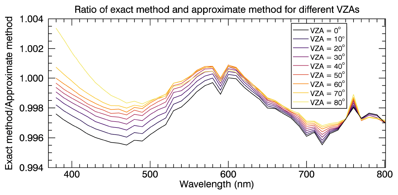
Figure 1 Ratio of scattered solar radiance spectra for the exact and approximate method for different VZAs, SZA = 90^∘ and RAA = 0^∘.

For the simulations with SCIATRAN, vertical profiles of atmospheric trace gases, pressure and temperature for northern mid-latitudes were used from the incorporated climatological database based on a 3-D chemical transport model (Sinnhuber et al., 2003). The effects of refraction are considered for both direct and scattered sunlight. The calculations were done neglecting the polarisation. A test considering polarisation for SZAs = 10 and 70^∘ and different viewing geometries resulted in a maximum relative difference of ≈ 1 % of the x and y chromaticity coordinates.

Simulations were performed for viewing geometries of SZAs = 10, 30, 50, 70, 80 and 90^∘ and VZAs = 0– 90^∘ in 10^∘ steps and RAAs = 0–180^∘ in 30^∘ steps.

A mono-modal log-normal particle size distribution was assumed for the implemented tropospheric and stratospheric aerosols:

$$\begin{array}{}\text{(1)}& n\left(r\right)={\displaystyle \frac{N_{\mathrm{0}}}{\sqrt{\mathrm{2}\mathit{\pi }}\cdot \ln \left(S\right)\cdot r}}\cdot \exp \left[-{\displaystyle \frac{(\ln r-\ln r_{\mathrm{m}}{)}^{\mathrm{2}}}{\mathrm{2}{\ln }^{\mathrm{2}}\left(S\right)}}\right],\end{array}$$

where N₀ is the total particle number density, S the geometric standard deviation of the distribution, r the particle radius and r_m the median radius. The corresponding input parameters for the Mie calculations carried out with the Mie code included in SCIATRAN are discussed in Sect. 3. Output of the simulations performed here are the intensities of the radiation in a wavelength range of 380–800 nm with a wavelength grid of 1 nm. In order to obtain the spectral distribution of the scattered solar radiation for an observer on the Earth's surface, the simulated spectra were multiplied with a solar irradiation spectrum (SORCE – Solar Radiation and Climate Experiment – data; LASP, 2003). For more detailed information on the radiative transfer model SCIATRAN we refer to, for example, Rozanov et al. (2014).

2.2 Chromaticity coordinates

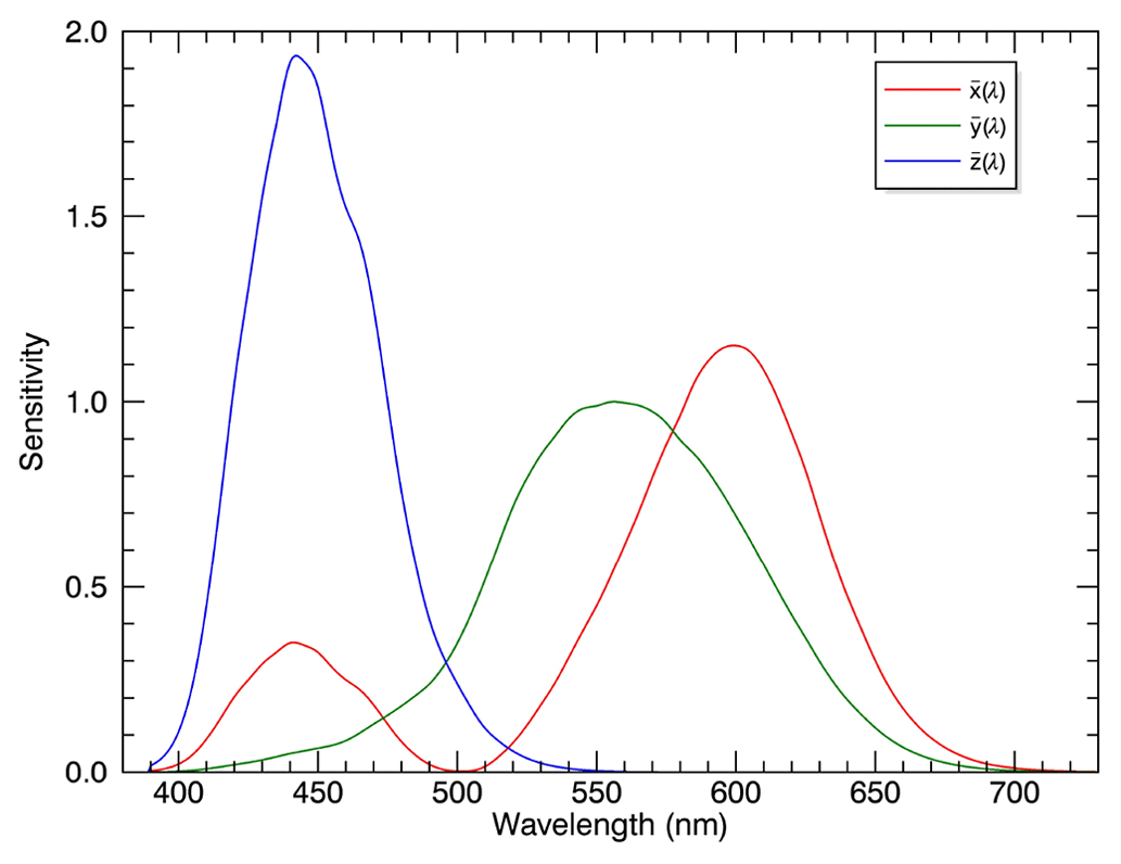
The CIE XYZ 1931 colour system enables the objective representation of colours in a two-dimensional coordinate system with the chromaticity coordinates x and y on the axes, the so-called CIE chromaticity diagram (e.g. Wyszecki and Stiles, 2000; CIE, 2004). Using the CIE colour matching functions $\stackrel{\mathrm{‾}}{x}\left(\mathit{\lambda }\right)$, $\stackrel{\mathrm{‾}}{y}\left(\mathit{\lambda }\right)$ and $\stackrel{\mathrm{‾}}{z}\left(\mathit{\lambda }\right)$ (compare Fig. 2), which describe the spectral sensitivity of the cone cells of the human eye, the CIE XYZ tristimulus values of a simulated spectrum I(λ) were determined by multiplying the simulated spectrum by these functions with subsequent integration (Billmeyer Jr. and Fairman, 1987):

$$\begin{array}{}\text{(2)}& {\displaystyle }X=\underset{\mathrm{380}\mathrm{nm}}{\overset{\mathrm{800}\mathrm{nm}}{\int }}I\left(\mathit{\lambda }\right)\stackrel{\mathrm{‾}}{x}\left(\mathit{\lambda }\right)\mathrm{d}\mathit{\lambda }\text{(3)}& {\displaystyle }Y=\underset{\mathrm{380}\mathrm{nm}}{\overset{\mathrm{800}\mathrm{nm}}{\int }}I\left(\mathit{\lambda }\right)\stackrel{\mathrm{‾}}{y}\left(\mathit{\lambda }\right)\mathrm{d}\mathit{\lambda }\text{(4)}& {\displaystyle }Z=\underset{\mathrm{380}\mathrm{nm}}{\overset{\mathrm{800}\mathrm{nm}}{\int }}I\left(\mathit{\lambda }\right)\stackrel{\mathrm{‾}}{z}\left(\mathit{\lambda }\right)\mathrm{d}\mathit{\lambda }.\end{array}$$

Figure 2 CIE colour matching functions of the cone cells of the human eye after Judd (1951) and Vos (1978).

The chromaticity values x and y were then calculated as follows:

$$\begin{array}{}\text{(5)}& x={\displaystyle \frac{X}{X+Y+Z}}y={\displaystyle \frac{Y}{X+Y+Z}}.\end{array}$$

For the representation in the CIE chromaticity diagram, the CIE XYZ tristimulus values were converted to standard RGB (sRGB). However, it should be noted that the displayed colours may vary depending on the output device. More information on colour modelling can be found in previous papers, e.g. Lange et al. (2023) and Wullenweber et al. (2021).

2.3 Determining the contribution of ozone to the blue colour of the sky

To determine the contribution of ozone to the blue colour of the sky for different viewing geometries, the corresponding chromaticity coordinates x and y were first calculated. Figure 3 shows an example of the representation in the CIE chromaticity diagram (enlarged) with SZA = 10^∘ and RAA = 0^∘ as well as VZAs = 10, 80, 86 and 90^∘ (Fig. 3a) and SZA = 90^∘ and RAA = 0^∘ as well as VZAs = 10, 40, 60 and 70^∘ (Fig. 3b), both for an observer on the Earth's surface. The “x” in the CIE chromaticity diagram (x = y = $\mathrm{1}/\mathrm{3}$) corresponds to the “white point”.

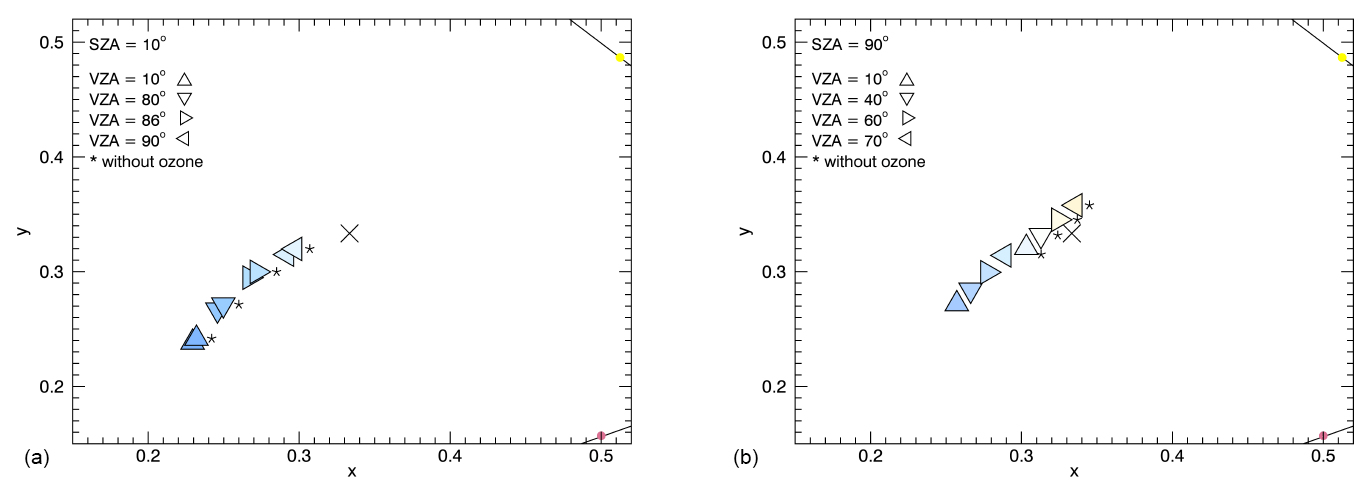
Figure 3 Example of the representation in the CIE chromaticity diagram (enlarged). (a) SZA = 10^∘, RAA = 0^∘, VZAs = 10, 80, 86, 90^∘. (b) SZA = 90^∘, RAA = 0^∘, VZAs = 10, 40, 60, 70^∘. Both for an observer on the Earth's surface.

To estimate the contribution of ozone to the blue colour of the sky, the next step was to calculate the (Euclidean) distances between the data point (with ozone d₁ and without ozone d₂) and the “white point” in the CIE chromaticity diagram. Subsequently, the difference between both distances was determined, divided by the distance d₁ (with ozone), yielding the relative difference r (d₁ is always greater than d₂):

$$\begin{array}{}\text{(6)}& {\displaystyle \frac{d_{\mathrm{1}}-d_{\mathrm{2}}}{d_{\mathrm{1}}}}=r.\end{array}$$

The calculated relative differences are colour-coded and displayed in polar diagrams in the following sections.

The method is not applicable for all cases. Figure 3b shows for VZAs = 60 and 70^∘, for example, viewing geometries where the method is inapplicable. That is generally the case for chromaticity coordinates corresponding to the green, yellow, orange and red colour regions of the CIE chromaticity diagram and can apply to one data point or both (with and without ozone); this covers all cases occurring in this work but not every theoretically possible one. Since the studies focus on the blue colour of the sky, these limitations occur mainly at large SZAs and at VZAs near the horizon. Deviations from this can appear due to changes in the total ozone column (TOC) and aerosol content (further discussed in the following section). Note that the fact that the method is not applicable in all cases does not affect the goals of the study, i.e. to determine the contribution of ozone to the blue colour of the sky, because the sky is not blue anymore in the cases that cannot be studied.

3 Results and discussion

The results in this section are based on the following assumptions, if not stated otherwise. For the particle size distribution and spectral extinction properties of the implemented tropospheric aerosol layer in the altitude range of 0–9 km, the “tropospheric” aerosol model from Shettle and Fenn (1979) was used. The aerosols consist of 70 % water-soluble components (ammonium and calcium sulfate and organics) and 30 % dust-like components with the following parameters: r_m = 33 nm, S = 1.4 and an aerosol optical depth (AOD) at 550 nm of 0.04 (Shettle and Fenn, 1979). The AOD of 0.04 at 550 nm is in the range of AOD values observed with the AERONET (Aerosol Robotic Network) photometer at the Institute of Physics of the University of Greifswald. In Shettle and Fenn (1979), the AOD is not predefined and can be adjusted accordingly using the number density N. The mono-modal log-normal particle size distribution of the tropospheric aerosols results from the elimination of larger particles from the model, since the particles above the boundary layer have a longer residence time and the larger particles settle due to gravity (Shettle and Fenn, 1979). For clear conditions, the “tropospheric model” is also valid for the boundary layer. More detailed information can be found in Shettle and Fenn (1979). It should be noted that the aerosol content in the troposphere is highly variable, and it is not possible to account for this variability within the scope of this work.

The stratospheric aerosol layer at 10–25 km altitude consists of sulfate particles with the following characteristics: r_m = 100 nm, S = 1.6 and AOD (550 nm) = 1.4 × 10⁻³. Other AODs for the stratosphere are also used in the following; see more details below. Accordingly, the total AOD of both aerosol layers is 0.0414 at 550 nm. For the TOC, 300 DU was first assumed.

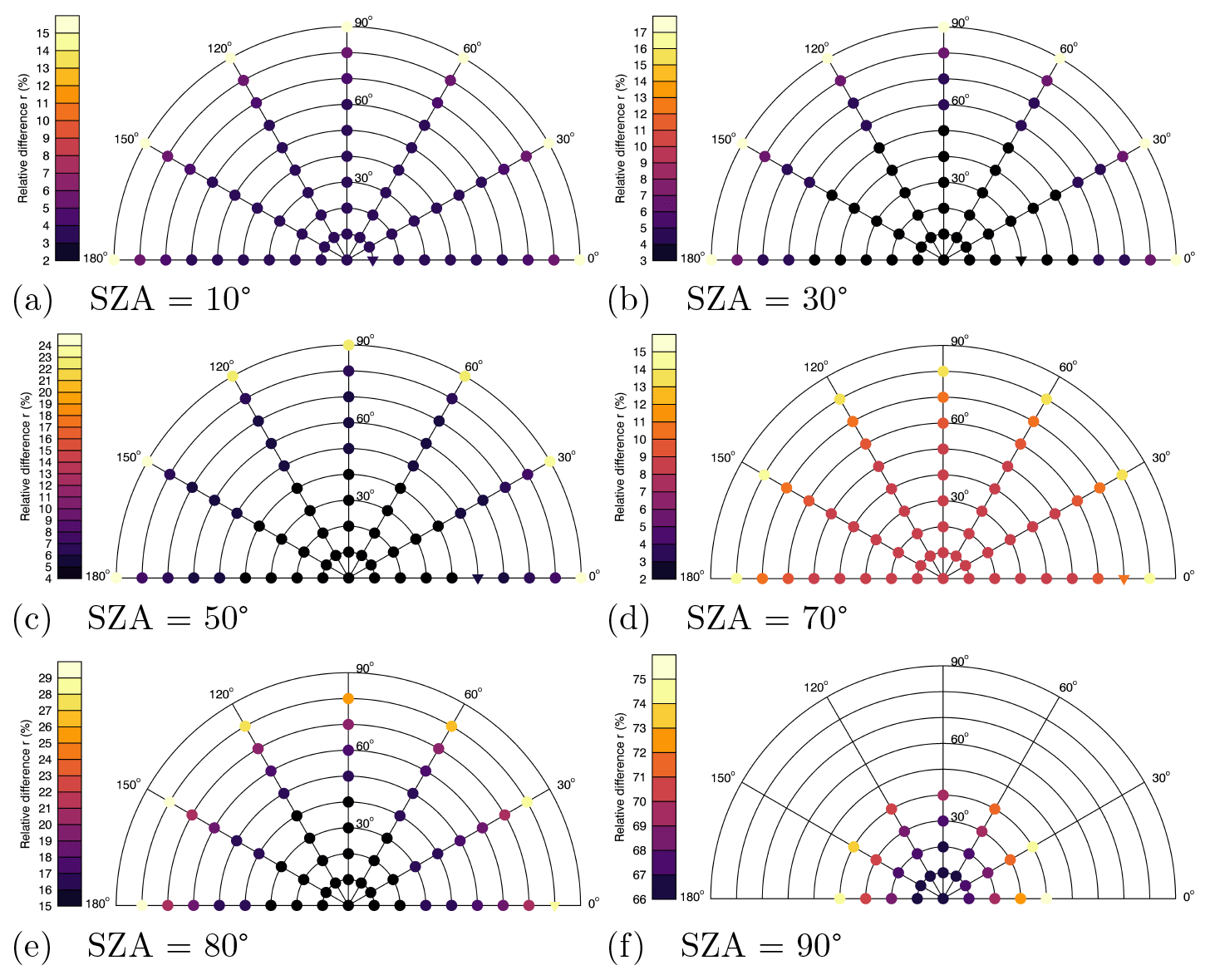
Figure 4 Polar diagrams for SZAs = 10^∘ (a), 30^∘ (b), 50^∘ (c), 70^∘ (d), 80^∘ (e) and 90^∘ (f) with the relative differences r colour-coded. The radius of the polar diagram corresponds to the VZA and the angle to the RAA (marked at the outer edge of the diagram). The missing values are due to the non-applicability of the method as described above.

Figure 4 shows polar diagrams for SZAs = 10^∘ (Fig. 4a), 30^∘ (Fig. 4b), 50^∘ (Fig. 4c), 70^∘ (Fig. 4d), 80^∘ (Fig. 4e) and 90^∘ (Fig. 4f) with the relative differences (see Eq. 6) colour-coded. The radius of the polar diagram corresponds to the VZA and the angle to the RAA (marked at the outer edge of the diagram). The upside-down triangle symbol in the diagrams indicates the observation geometry where the ground-based observer is looking directly into the Sun. Note that the simulations performed here consider only the scattered and not the directly transmitted sunlight. Furthermore, due to the azimuthal symmetry of the radiation field, the RAAs between 180 and 360^∘ lead to the same simulation results as the corresponding RAAs between 180 and 0^∘. Therefore, only results for RAAs between 0 and 180^∘ are shown in the following. Missing values within this RAA range are due to the non-applicability of the method.

For SZA = 10^∘ (Fig. 4a) small relative differences are found as expected, i.e. a minor influence of ozone on the blue colour of the sky, which increases with increasing VZA from 3 % (VZA = 0^∘) to 15 % (VZA = 90^∘), with absolute differences of 0.004 (VZA = 0^∘) and 0.0065 (VZA = 90^∘). The first change in the relative differences can be seen at VZA = 70^∘. Similar results are observed for SZA = 30^∘ (Fig. 4b), with 3 % relative difference up to VZA = 50^∘ and 17 % at VZA = 90^∘ (absolute differences: 0.005, VZA = 0^∘ and 0.007, VZA = 90^∘). For both SZAs, no RAA-dependent change in the ozone influence is found.

At larger SZAs, i.e. longer light paths through the atmosphere, the ozone influence increases, and thus the values of the relative difference increase as well (compare Fig. 4c–f). For SZA = 50^∘, the contribution of ozone is 4 % at the zenith (VZA = 0^∘) (up to VZA = 40^∘) and 24 % at the horizon (VZA = 90^∘) (Fig. 4c). The relative difference for VZA = 90^∘ varies here slightly with the RAA. For RAAs = 0, 150 and 180^∘ the value is 24 %; for RAA = 30^∘ it is 23 %; and for RAAs = 60, 90 and 120^∘ the value of the relative difference is 22 %. In comparison, the contribution of ozone to the blue colour for an SZA of 70^∘ is 8 % at the zenith (up to VZA = 50^∘) and ≈ 14 % at VZA = 80^∘ (for SZA = 50^∘ and VZA = 80^∘ it is 8 %). The value of the relative difference at VZA = 80^∘ also varies with the RAA here (see Fig. 4d).

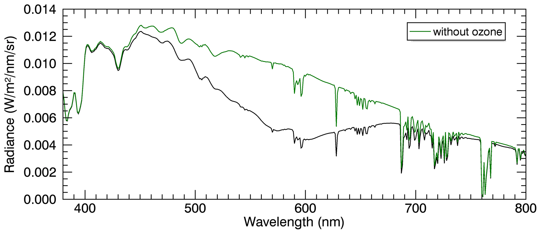
Figure 5 Scattered solar radiation spectra for SZA = 90^∘ and VZA = 0^∘ with TOC = 300 DU (black line) and TOC = 0 DU (green line).

Figure 4e and f show polar diagrams for SZA = 80^∘ (Fig. 4e) and SZA = 90^∘ (Fig. 4f). The values of the relative difference calculated for SZA = 80^∘ range from 15 % (VZA = 0^∘) to ≈ 29 % (VZA = 80^∘), depending on the RAA. For SZA = 90^∘ the relative differences and thus the contribution of ozone increase significantly. At the zenith, ozone accounts for 66 % of the blue colour (absolute difference: 0.065). This is in good agreement with the estimate of Hulburt (1953) of $\mathrm{2}/\mathrm{3}$ ozone influence at the zenith at sunset with a TOC of 240 DU. Our calculations for TOC = 240 DU, SZA = 90^∘ and VZA = 0^∘ yielded a value of 60 % (not shown). However, this is still close to the ozone contribution determined by Hulburt. Also for SZA = 90^∘, the contribution of ozone increases with increasing VZA with a maximum value of 75 % at VZA = 40^∘ and RAA = 0^∘. The relative differences for the RAAs of 30–150^∘ are slightly smaller compared to RAA = 0^∘ and 180^∘. Figure 5 shows the corresponding scattered solar radiation spectra for SZA = 90^∘ and VZA = 0^∘ with TOC = 300 DU (black line) and TOC = 0 DU (green line). The effect of the ozone Chappuis bands (centred around 600 nm) on the scattered radiance spectra is quite pronounced, consistent with the large influence of ozone on the sky colour of this viewing geometry.

Summarising, the results are in good agreement with the work of Hulburt (1953), and they significantly extend Hulburt's work in different ways. Ozone has been shown to strongly affect the colour of the sky not only for the zenith viewing geometry and SZA = 90^∘, but also for larger VZAs. In addition, it was shown that ozone also plays a role for the sky colour for smaller values of the SZA, with the ozone influence increasing with both increasing VZA and SZA.

3.1 Influence of the total ozone column

For all calculations shown so far, a TOC of 300 DU was assumed. Figure 6 shows the resulting relative differences (compare Eq. 6) for SZAs = 10^∘ (Fig. 6a and b), 50^∘ (Fig. 6c and d) and 90^∘ (Fig. 6e and f) with TOC = 500 DU (Fig. 6a, c and e) and TOC = 100 DU (Fig. 6b, d and f). TOC values of 100 DU and 500 DU were chosen because this range essentially covers all possible values occurring in the Earth's atmosphere.

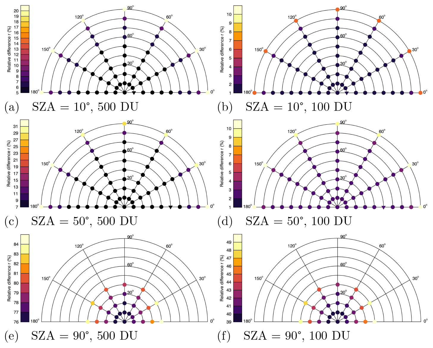
Figure 6 First row: polar diagrams for SZA = 10^∘, TOC = 500 DU (a) and TOC = 100 DU (b). Second row: polar diagrams for SZA = 50^∘, TOC = 500 DU (c) and TOC = 100 DU (d). Third row: polar diagrams for SZA = 90^∘, TOC = 500 DU (e) and TOC = 100 DU (f) with the relative differences r colour-coded.

With a TOC of 100 DU and SZA = 10^∘, the contribution of ozone is reduced to 1 % at the zenith (up to VZA = 70^∘) and 6 % at the horizon (Fig. 6b). The absolute differences are 0.001 for VZA = 0^∘ and 0.0025 for VZA = 90^∘. Assuming a larger TOC of 500 DU (Fig. 6a), the ozone contribution increases to 5 % at the zenith (up to VZA = 50^∘) and 20 % at the horizon (absolute differences: 0.006, VZA = 0^∘ and 0.0095, VZA = 90^∘). In comparison, the ozone contribution for TOC = 300 DU is 3 % at the zenith and 15 % at the horizon (compare Fig. 4a). At a SZA of 50^∘ (Fig. 6c and d), the influence of ozone increases as expected due to the longer light path through the atmosphere. For TOC = 500 DU (Fig. 6c), the relative differences range from 7 % (VZA = 0^∘) to ≈ 31 % (VZA = 90^∘). For a smaller TOC (100 DU) (Fig. 6d), the relative differences are 2 % for VZA = 0^∘ and ≈ 10 % for VZA = 90^∘. The exact values of the relative difference at VZA = 90^∘ depend on the RAA.

While the contribution of ozone to the blue colour of the zenith is 66 % for SZA = 90^∘ and 300 DU (as illustrated in Fig. 4f), the contribution increases to 76 % for 500 DU (Fig. 4e) (absolute difference: 0.108) and correspondingly decreases to 39 % for 100 DU (Fig. 4f) (absolute difference: 0.022) (see Fig. 6e and f). The relative differences for the VZAs 10–40^∘ vary with the RAA. For 100 DU (Fig. 6f), the maximum value is 49 % and for 500 DU (Fig. 6e) 84 % for RAA = 0^∘ and VZA = 40^∘; note that the approach does not work for larger VZAs.

The plots show that the contribution of ozone to the blue colour of the sky for different viewing geometries depends strongly on the assumed TOC. The contribution of ozone at 100 DU is nearly negligible for small SZAs (see Fig. 6b and d). As expected, the values of the relative difference, i.e. the influence of ozone, increase for larger TOCs (e.g. 500 DU) and decrease for smaller TOCs (e.g. 100 DU); compare Fig. 7.

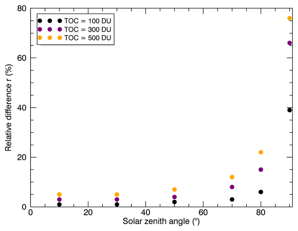
Figure 7 Relative difference (see Eq. 6) as a function of the SZA for different TOCs: 100, 300 and 500 DU. The viewing geometry is the following: VZA = 0^∘; SZAs = 10, 30, 50, 70, 80, 90^∘; and RAA = 0^∘.

3.2 Aerosol effects

In order to test how the contribution of ozone to the blue colour of the sky changes with increased aerosol content, the following stratospheric aerosol scenario was assumed for the calculations: r_m = 250 nm, S = 1.6 and a stratospheric aerosol optical depth (SAOD) of 0.1 at 550 nm. For comparison, the maximum globally averaged SAOD at 550 nm after the eruption of Mt. Pinatubo in June 1991 was about 0.15 (e.g. McCormick et al., 1995). The parameters of the tropospheric aerosols remain unchanged. The total AOD of both layers is 0.14 (at 550 nm), and a TOC of 300 DU was assumed. The symbols in the following polar diagrams shown in grey illustrate comparatively high values of the relative difference and are indicated separately for the sake of readability and clarity.

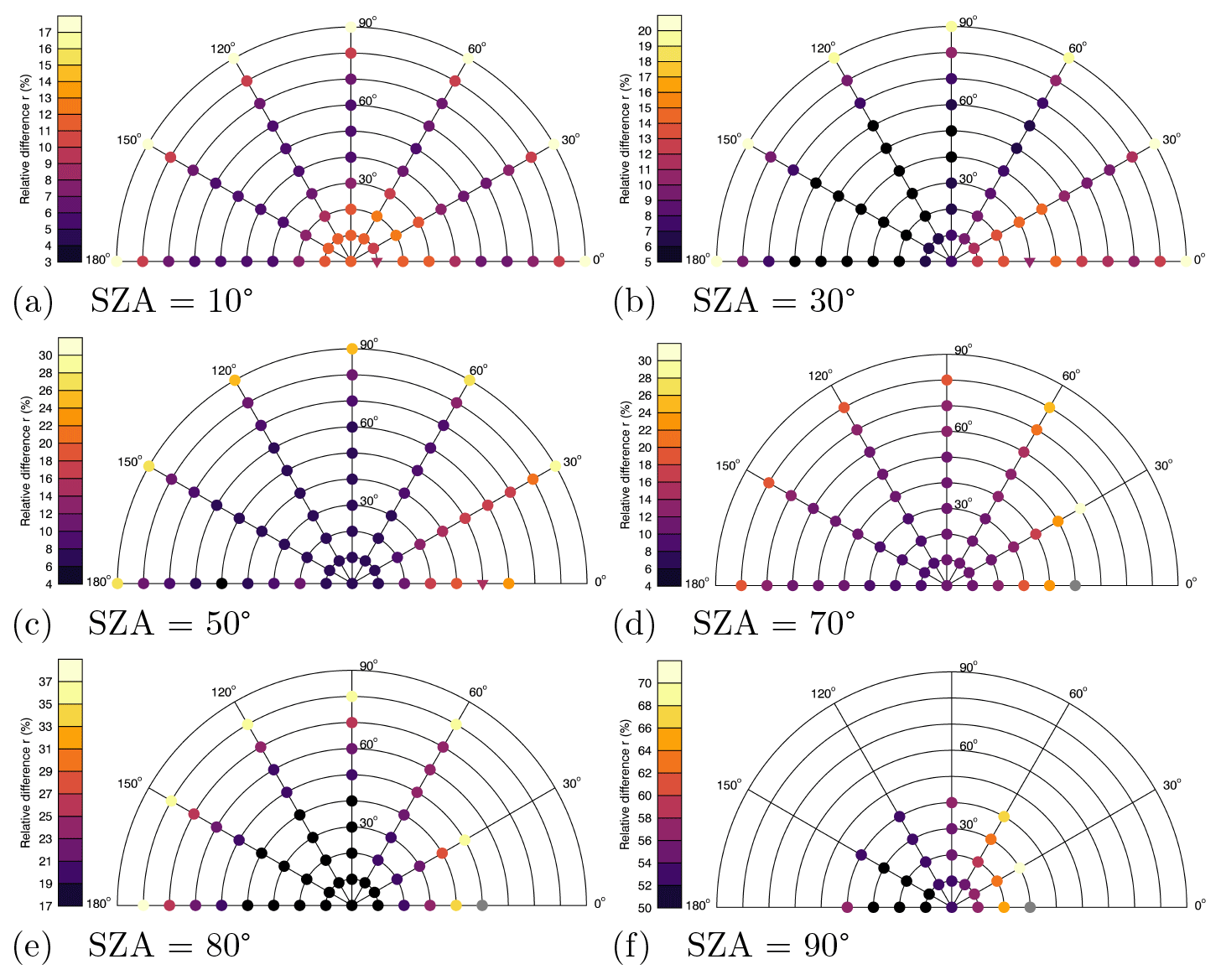
Figure 8 Polar diagrams for SZAs = 10^∘ (a), 30^∘ (b), 50^∘ (c), 70^∘ (d), 80^∘ (e) and 90^∘ (f) with the relative differences r colour-coded. The calculations were carried out for the enhanced stratospheric aerosol content scenario with SAOD = 0.1 (550 nm). For SZA = 70^∘ (d), RAA = 0^∘ and VZA = 50^∘ the value of the relative difference is 37 %. For SZA = 80^∘ (e), RAA = 0^∘ and VZA = 50^∘ the value of the relative difference is 52 %. For SZA = 90^∘ (f), RAA = 0^∘ and VZA = 30^∘ the value is 76 %.

Figure 8a and b show the results for SZA = 10^∘ (Fig. 8a) and SZA = 30^∘ (Fig. 8b). For both SZAs, the relative differences (compare Eq. 6) depend strongly on the RAA. While no RAA-dependent change in ozone contribution is observed in Fig. 4 for SZAs = 10^∘ (Fig. 4a) and 30^∘ (Fig. 4b) (“baseline aerosol scenario”), here the relative differences can vary with the RAA by up to 3 %. For SZA = 10^∘, ozone accounts for 11 % of the blue colour at the zenith. For SZA = 30^∘ the contribution decreases to 8 %, but the maximum contribution (considering all VZA–RAA combinations) of ozone is still larger than for the SZA of 10^∘. At the horizon, the relative differences are 17 % for a SZA of 10^∘ and 20 % for SZA = 30^∘ and RAAs of 0^∘, 30^∘, 150^∘ and 180^∘.

The relative differences for a SZA of 50^∘ (Fig. 8c) range from 6 % at VZA = 0^∘ to ≈ 28 % (RAA = 30^∘) –25 % (RAA = 90^∘) at VZA = 90^∘. In comparison, the ozone contribution at the zenith for a SZA of 70^∘ (Fig. 8d) is 10 %. The grey symbol at SZA = 70^∘, RAA = 0^∘ and VZA = 50^∘ corresponds to a relative difference of 37 %. With 37 % the ozone contribution to the blue colour of the sky is comparatively large for this viewing geometry. For a RAA of 0^∘, the ground-based observer looks in the sunward direction, but with VZA = 50^∘ not directly into the Sun. It can be assumed that the forward peak of the aerosol scattering plays an important role, but a final explanation cannot be given at this point. Figure 8e and f show results for the calculations with the Sun 10^∘ above the horizon (Fig. 8e) and at the horizon (Fig. 8f). The ozone contribution for SZA = 80^∘ and VZA = 0^∘ is 17 % here and increases to 36 % (RAAs 0–150^∘) at VZA = 80^∘. The viewing geometry of SZA = 80^∘, RAA = 0^∘ and VZA = 50^∘ corresponds to a value of 52 %. For SZA = 90^∘ a significant increase in ozone influence is also observed for the enhanced stratospheric aerosol scenario. Here the contribution of ozone to the blue colour at the zenith is 53 % (absolute difference: 0.062) and at VZA = 40^∘ 67 % (maximum value over all RAAs).

The calculations for SZA = 90^∘ with the “baseline aerosol scenario” (Fig. 4f) and the enhanced stratospheric aerosol content scenario (Fig. 8f) show that more stratospheric aerosols reduce the influence of ozone on the blue colour of the sky at and near the zenith. For instance, the value of the relative difference for the “baseline aerosol scenario” at the zenith is 66 %, which is reduced to 53 % with more stratospheric aerosols and the specific aerosol particle size distribution assumed here. However, this is only the case for the SZA of 90^∘, since at the other SZAs shown here, the contribution of ozone is larger with more stratospheric aerosols (compare, for example, Fig. 4a and Fig. 8a). Nevertheless, the differences between the relative differences in both scenarios decrease with increasing VZA (exact values also depend on the RAA) and SZA – especially for SZAs of 10–80^∘. This supports the conclusion that the light path through the atmosphere, which increases with increasing SZA, is crucial for this effect. Note that there is no final explanation for this effect at this point, but the following may represent a possible explanation. With SZAs of 10–80^∘ and the enhanced aerosol content of the stratospheric aerosol layer (10–25 km), the scattered sunlight perceived by the observer on the Earth's surface comes mainly from this altitude and thus has a longer light path through the stratospheric ozone layer, resulting in higher relative differences, i.e. higher ozone contributions. With the Sun at the horizon, the scattered sunlight comes mainly from higher altitudes, resulting in a reduction in the ozone contribution. This is a potential explanation that we cannot prove conclusively. Simulations were also carried out for two other stratospheric aerosol scenarios, one with r_m = 450 nm, S = 1.6 and SAOD = 0.1 (550 nm) and the other with r_m = 250 nm, S = 1.6 and SAOD = 0.2 (550 nm), which lead to similar results for SZA = 90^∘ (not shown).

In Adams et al. (1974) they concluded that with “ten times normal aerosol amount” (vertical optical thickness between 2 and 3.5) the blue of the zenith and near the zenith sky decreases; i.e. the spectral purity is reduced. The spectral purity indicates how monochromatic a colour is; for example, a point near the “white point” in the CIE chromaticity diagram has a low spectral purity, whereas a point near the spectral arc of the CIE chromaticity diagram has a high spectral purity. Adams et al. (1974) performed these calculations only for SZAs of 90–96^∘ and considered just single scattering, but the shift to larger x values can also be observed in the present calculations for the enhanced aerosol content scenario at all SZAs (not shown).

For the “baseline aerosol scenario”, which corresponds to stratospheric aerosol background conditions, it is a valid approximation that the remaining contribution, besides the calculated ozone contribution, is due to Rayleigh scattering. This cannot be directly concluded for the enhanced stratospheric aerosol content scenario, since aerosols also have a contribution, as shown above.

In addition, we also tested the effect of the surface albedo and the height of the observer. A test with different values of the surface albedo (0.1–0.5) led to a maximum relative difference in the x and y chromaticity coordinates of less than 1 %. For an observer at an altitude of 10 km, the contribution of ozone to the blue colour of the sky is 3 % for SZA = 10^∘ and VZA = 0^∘ and 16 % for VZA = 90^∘. For SZA = 90^∘ and VZA = 0^∘ the contribution is 78 %. With an observation height of 10 km an increase in the ozone contribution to the blue colour of the sky can be seen (compare with Fig. 4), which is consistent with expectations, since at an altitude of 10 km most of the ozone is still above this altitude, and Rayleigh scattering is reduced.

4 Conclusions

With the radiative transfer model SCIATRAN, the CIE XYZ 1931 colour system and the new approach used in the present work we quantified the contribution of ozone to the blue colour of the sky for different viewing geometries. We were able to demonstrate quantitatively that the blue colour of the sky cannot be solely attributed to Rayleigh scattering. Therefore, our work represents an additional confirmation of previous studies on the influence of ozone on the blue colour of the sky, although our work is based on a new quantitative method. The calculations show that ozone contributes to the blue colour of the sky also beyond the zenith viewing geometry and SZA = 90^∘. The calculations also show that the exact contribution of ozone is highly dependent on the assumed TOC. Moreover, the influence of ozone increases with increasing TOC, VZA and SZA. Ozone also contributes to the blue sky at small SZAs, although the contribution is found to be minor. In addition, the results for SZA = 90^∘ are in good agreement with Hulburt's estimation of $\mathrm{2}/\mathrm{3}$ ozone influence at the zenith at sunset. With more aerosols, the ozone contribution at the zenith is reduced to 53 % for SZA = 90^∘. Overall, the study of the influence of enhanced aerosol shows complex behaviour, as the ozone contribution is larger at small SZAs than in the “baseline aerosol scenario” and smaller at SZA = 90^∘. Calculations with different values of the surface albedo lead to minor effects on the ozone contribution to the blue colour of the sky. Furthermore, at an observation height of 10 km, an increase in the ozone influence is observed.