A colorful look at climate sensitivity

The radiative response to warming and to changing concentrations of CO₂ is studied in spectral space. If, at a particular wavenumber, the emission temperature of the constituent controlling the emission to space does not change its emission temperature, as is the case when water vapor adopts a fixed relative humidity in the troposphere or for CO₂ emissions in the stratosphere, spectral emissions become independent of surface temperature, giving rise to the idea of spectral masking. This way of thinking allows one to derive simple, physically informative, and surprisingly accurate expressions for the clear-sky radiative forcing, the radiative response to warming, and hence climate sensitivity. Extending these concepts to include the effects of clouds leads to the expectation that (i) clouds dampen the clear-sky response to forcing; (ii) diminutive clouds near the surface, which are often thought to be unimportant, may be effective at enhancing the clear-sky sensitivity over deep moist tropical boundary layers; (iii) even small changes in high clouds over deep moist regions in the tropics make these regions radiatively more responsive to warming than previously believed; and (iv) spectral masking by clouds may contribute substantially to polar amplification. The analysis demonstrates that the net effect of clouds on warming is ambiguous, if not moderating, justifying the assertion that the clear-sky (fixed relative humidity) climate sensitivity – which, after accounting for surface albedo feedbacks, we estimate to be about 3 K – provides a reasonable prior for Bayesian updates accounting for how clouds are distributed, how they might change, and deviations associated with changes in relative humidity with temperature. These effects are best assessed by quantifying the distribution of clouds and water vapor and how they change in temperature rather than geographic space.

1 Introduction

In recent years, conceptualizing the effects of thermal infrared radiation in spectral space has helped advance our understanding of many basic aspects of Earth's energy balance and how it responds to forcing. For instance, a consideration of the differential spectral response of outgoing longwave radiation (OLR) to warming has proved crucial to understanding why OLR varies approximately linearly with temperature (Koll and Cronin, 2018) and how clear-sky radiative cooling is distributed through the depth of the troposphere (Jeevanjee and Fueglistaler, 2020; Hartmann et al., 2022). A spectral treatment of thermal infrared radiation is also necessary to understand how radiation responds to forcing – in the form of increasing concentrations of atmospheric CO₂ (Wilson and Gea-Banacloche, 2012; Seeley, 2018; Jeevanjee et al., 2021b) – and how it maintains an ability to respond to warming at very warm temperatures (Kluft et al., 2021; Seeley and Jeevanjee, 2021). All of the above studies helped answer important questions by abandoning the idea that atmospheric radiative transfer could usefully be thought about as broadband or gray.

The chief advantage of a gray atmosphere is heuristic. Conceptualizing the entirety of radiative transfer in terms of a single emission height is a considerable simplification. In a gray world, intuition as to how the atmosphere responds to changes can be built around an understanding of what controls this emission height. This “gray” way of thinking still greatly influences how we quantify changes to Earth's radiant energy budget, for instance when quantifying clear- and cloudy-sky feedbacks. It turns out that thinking about radiative transfer more colorfully is not that much more difficult, and by managing to do so it becomes possible to anticipate and quantify radiative responses to forcing¹ that gray thinking either misrepresents or cannot explain. The chief simplification in treating the more colorful atmosphere is to recognize that different colors are controlled by different constituents, and, to a good degree of approximation, these constituents can be categorized as sensitive or invariant emitters of thermal radiation. Quantification of their net effect then follows quite simply from allowing invariant emitters to mask the response of sensitive emitters in proportion to their (the sensitive emitters') optical depth, something we call spectral masking.

The ideas presented here were developed in lectures on the greenhouse effect the first author gave at the Universität Hamburg in the fall of 2021. Many had their origins in joint work with the second author. Subsequently, we became aware that others were, or had been, thinking along similar lines to understand cloud-free atmospheres. For instance, the simple model of CO₂ forcing discovered and presented in those lectures had been found independently, and much earlier, by Wilson and Gea-Banacloche (2012) and has since been elaborated upon further and more thoroughly by Seeley (2018), Jeevanjee et al. (2021b), and Romps et al. (2022). Likewise, the ideas related to the clear-sky radiative response were being developed independently by Jeevanjee et al. (2021a), McKim et al. (2021), Colman and Soden (2021), and Koll et al. (2023). In retrospect, these studies do much of the heavy lifting that some readers would like to see by way of justifying some of the approximations we make. This allows us to focus on showing how this colorful way of thinking can be condensed into a heuristic that helps us think about climate sensitivity and the role of clouds more broadly. In this sense, our work is intended less as a replacement for rigorous treatment of radiative transfer and more as a way to understand the results of such computations.

The outline of the paper is as follows: after introducing the data sources and community tools used, the basic ideas are introduced in Sect. 3. These are used to derive estimates and provide an understanding of Earth's clear-sky climate sensitivity and its components in Sect. 4. This provides a basis for thinking about Earth's equilibrium climate sensitivity more broadly (Sect. 5) and for better understanding the role of clouds in its determination. Conclusions and an outlook are presented in Sect. 6

2 Preliminaries

2.1 Data

Absorption spectra of selective absorbers, here CO₂ and H₂O, are taken from the catalog used for the Atmospheric Radiative Transfer Simulator, ARTS (Buehler et al., 2018; Eriksson et al., 2011). ARTS includes treatments of line broadening – with the treatment of the foreign broadening appropriate for Earth's atmosphere and a representation of continuum absorption following the approach of Clough et al. (1989, 2005) as modified by Mlawer et al. (2012). Other data sources include monthly mean, gridded ($\mathrm{0.25}{}^{\circ }\times \mathrm{0.25}{}^{\circ }$) near-surface (2 m) air temperatures, and column water vapor for the 240 months between 2001 and 2021, and these are taken from reanalyses of meteorological data (ERA5, Hersbach et al., 2019). Cloud data are based on measurements using the AATSR instrument which flew on ENVISAT (Poulsen et al., 2019). The record extends from May 2002 through April 2012, and level-3 cloud top temperature and cloud fraction are used.

2.2 Terminology and basic concepts

Concepts are developed for understanding the emission of terrestrial radiation, 99 % of which is emitted in the 50 to 2000 cm⁻¹ wavenumber (denoted by ν) interval. This is sometimes referred to as the longwave or thermal infrared part of the electromagnetic spectrum.

Table 1 Main symbols used in this study. Many are further specified by subscripts, with e denoting emission, sfc denoting surface, cp denoting cold point, cs denoting clear sky, cld denoting cloud, and v denoting vapor.

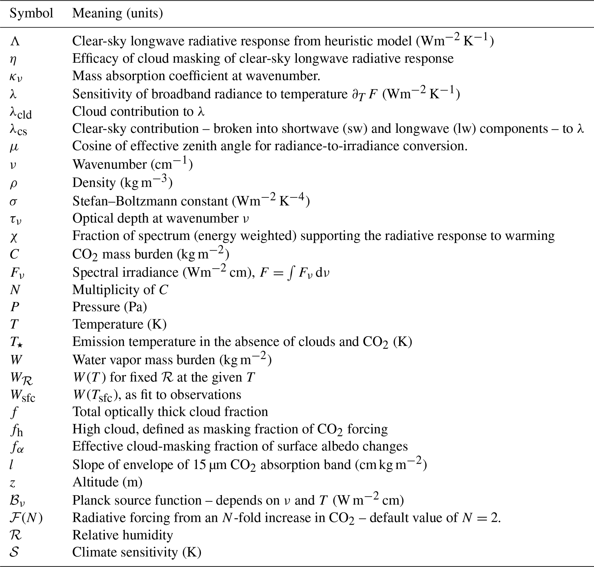
We adopt terminology (see also Table 1) that will be standard for many readers. The Planck source function is denoted by ℬ_ν and depends on wavenumber ν and temperature T. The spectral irradiance is denoted by F_ν and, unless indicated otherwise, is assumed to describe the outgoing thermal irradiance at the top of the atmosphere. The mass absorption cross-section κ_ν,x refers to a constituent x (either c for carbon dioxide or v for water vapor) whose density is denoted by ρ_x.

The optical depth between two heights z₁ and z₂ is denoted by ${\mathit{\tau }}_{\mathit{\nu },\mathrm{x}}(z_{\mathrm{1}},z_{\mathrm{2}})$ and defined as

$$\begin{array}{}\text{(1)}& {\mathit{\tau }}_{\mathit{\nu },\mathrm{x}}(z_{\mathrm{1}},z_{\mathrm{2}})=\underset{z_{\mathrm{1}}}{\overset{z_{\mathrm{2}}}{\int }}{\mathit{\kappa }}_{\mathit{\nu },\mathrm{x}}{\mathit{\rho }}_{\mathrm{x}}\mathrm{d}z\approx {\stackrel{\mathrm{‾}}{\mathit{\kappa }}}_{\mathit{\nu },\mathrm{x}}{M}_{\mathrm{x}}(z_{\mathrm{1}},z_{\mathrm{2}}).\end{array}$$

The approximation defines the path-integrated mass burden of x, denoted M_x, and a mean mass absorption cross-section, denoted ${\stackrel{\mathrm{‾}}{\mathit{\kappa }}}_{\mathit{\nu },\mathrm{x}}$. Hereafter, we denote the partial water vapor column burden M_v by W and the partial CO₂ burden M_c by C. W and C are equal to their respective column burdens when the path is taken to extend through the entirety of the atmosphere. The effective mass absorption coefficient includes the effects of continuum absorption and pressure broadening by adopting a single value at an effective pressure and temperature, $(P,T)=(\mathrm{850}\mathrm{h}\mathrm{Pa},\mathrm{280}\mathrm{K})$. An exception is for the case of CO₂, as used in estimates of the forcing, for which we adopt values $(P,T)=(\mathrm{500}\mathrm{hPa},\mathrm{255}\mathrm{K})$ to be more representative of the levels where the forcing establishes itself. Reducing the effective pressure and temperature for H₂O to $(P,T)=(\mathrm{700}\mathrm{hPa},\mathrm{270}\mathrm{K})$ changes estimates of the radiative response by about 2 %.

The transmissivity through an absorber x is given as $e^{-{\mathit{\tau }}_{\mathit{\nu },x}/\mathit{\mu }}$, where μ is the diffusivity factor. It is introduced by taking an effective zenith angle θ to scale the path length by ${\mathit{\mu }}^{-\mathrm{1}}=(\cos \mathit{\theta }{)}^{-\mathrm{1}}$ through the medium and thereby apply an equation originally valid for radiances to irradiances. The value of θ depends on the optical depth (Armstrong, 1968), but a value of $\mathit{\theta }=\mathrm{53}{}^{\circ }$ roughly corresponds to the average for optical depths uniformly distributed between 0 and 1, resulting in the commonly adopted value of ${\mathit{\mu }}^{-\mathrm{1}}=\mathrm{1.6}$. Beer's law thus becomes

$$\begin{array}{}\text{(2)}& F_{\mathit{\nu }}\left(z\right)=\mathit{\pi }{e}^{-{\mathit{\tau }}_{\mathit{\nu },\mathrm{x}}(z,z_{\mathrm{e}})/\mathit{\mu }}{\mathcal{B}}_{\mathit{\nu }}\left(T_{\mathrm{e}}\right),\end{array}$$

where subscript e denotes the emission value of a particular variable, e.g., height z_e or temperature T_e.

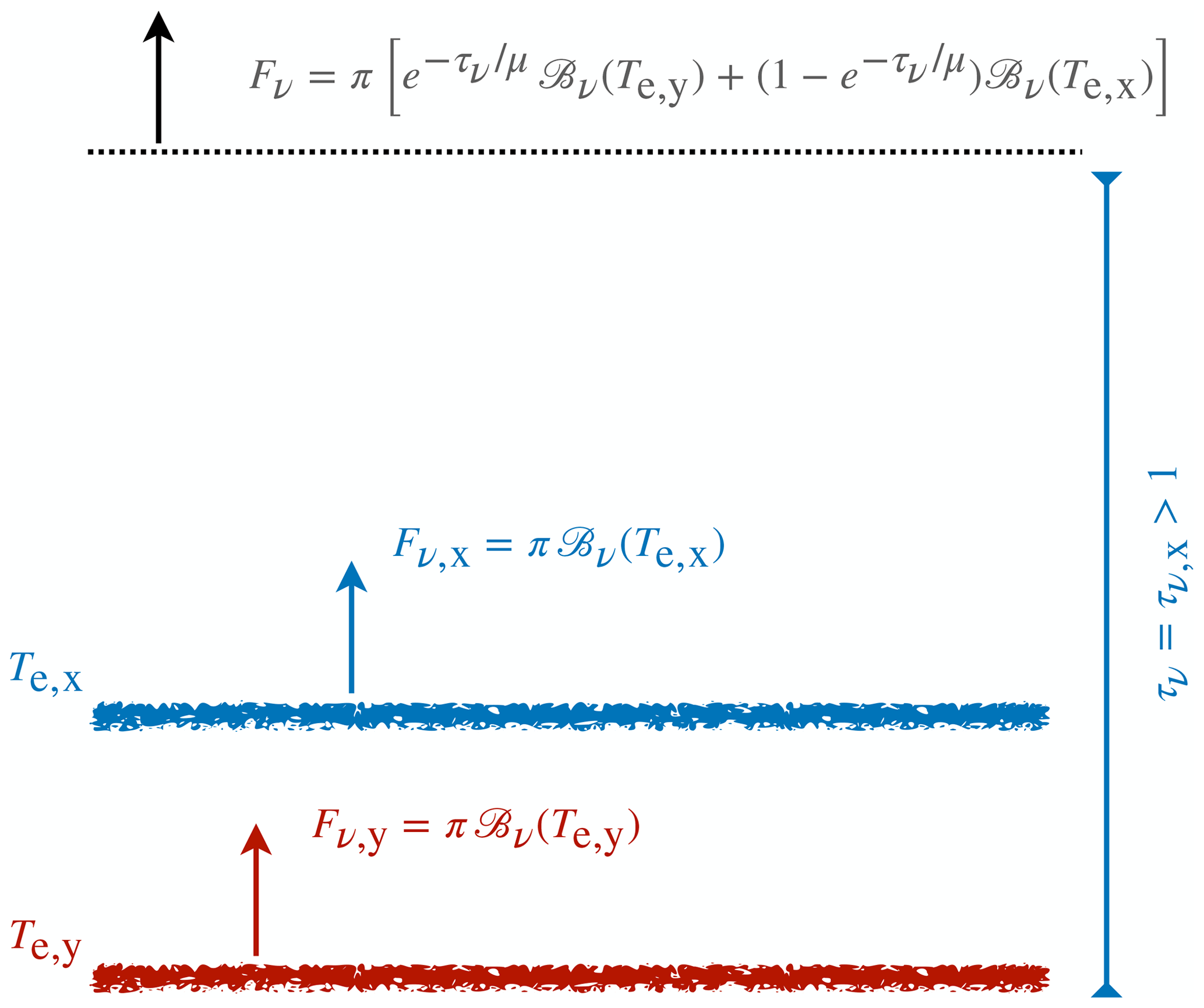
Figure 1 Schematic of simplified treatment of irradiances originating from two sources, denoted by x and y, with each emitting as a black body (ℬ_ν denotes the Planck source function) from a height where their respective optical depths τ_x,y (as measured from space) are at unity. The factor μ in the transmissivity (exponential terms) is the diffusivity factor that arises in converting radiances to irradiances.

3 Heuristics

The colorful ansatz amounts to the very simple and rather standard idea that emission to space at any given wavenumber is controlled by the emission temperature of the atmospheric constituent that first becomes optically thick at that wavenumber and that emission changes depend on how that absorber changes. We formalize this idea with the help of Fig. 1, which outlines how we smoothly weight the emissions from two absorbers (the lower one could be the surface) based on the optical thickness of the absorber which dominates the atmospheric emissions. Mathematically,

$$\begin{array}{}\text{(3)}& F_{\mathit{\nu }}=\mathit{\pi }\left[e^{-{\mathit{\tau }}_{\mathit{\nu },\mathrm{x}}/\mathit{\mu }}{\mathcal{B}}_{\mathit{\nu }}\left(T_{\mathrm{e},\mathrm{y}}\right)+\left(\mathrm{1}-e^{-{\mathit{\tau }}_{\mathit{\nu },\mathrm{x}}/\mathit{\mu }}\right){\mathcal{B}}_{\mathit{\nu }}\left(T_{\mathrm{e},\mathrm{x}}\right)\right],\end{array}$$

where x is the dominant absorber and becomes optically thick at some temperature $T_{\mathrm{e},\mathrm{x}}=T_{\mathrm{1}}$. The second absorber, or possibly surface, emits at the temperature $T_{\mathrm{e},\mathrm{y}}=T_{\mathrm{2}}>T_{\mathrm{1}}$ at which it becomes optically thick. A simple variant of this model, one that perhaps better illustrates the way of thinking it formalizes, is the “first-to-1” model², which simply replaces the transmissivity by 0 or 1 depending on whether or not ${\mathit{\tau }}_{\mathit{\nu },\mathrm{x}}>\mathrm{1}$.

To help us understand how F_ν responds to changes in the surface temperature T_sfc, thermal emissions at a given wavenumber are classified as arising from either a sensitive or T_sfc-invariant emitter.

Sensitive emitters

are ones whose emission temperatures change with T_sfc, such that $\mathit{\delta }{T}_{\mathrm{e},\mathrm{x}}=\mathit{\gamma }\mathit{\delta }{T}_{\mathrm{sfc}}$, with γ>0 being a proportionality constant.

Invariant emitters

are ones whose emission temperature is independent of T_sfc so that $\mathit{\delta }{\mathcal{B}}_{\mathit{\nu },\mathrm{x}}=\mathrm{0}$.

The surface, at all wavenumbers, is an obvious example of a sensitive emitter, with γ=1. At wavenumbers where it becomes optically thick in the troposphere, CO₂ also behaves like a sensitive emitter. In that case, following a moist adiabat, γ>1. Its precise value depends on how high in the troposphere its emission originates. To the extent that the water vapor path is only a function of temperature – something Jeevanjee et al. (2021a) call Simpson's law – it behaves as an invariant emitter. Likewise, to the extent that the stratosphere adjusts its temperature to maintain radiative equilibrium, CO₂ emissions from the stratosphere act as an invariant emitter.

The simple model, Eq. (3), and the concepts introduced here are not intended as a replacement for radiative transfer modeling. Their purpose is mainly to formalize the selection of a dominant emitter at a given wavenumber and to show how this knowledge (when combined with the essential properties of that emitter) proves to be surprisingly informative about how irradiances will change with warming or forcing, for instance as calculated by more complex models.

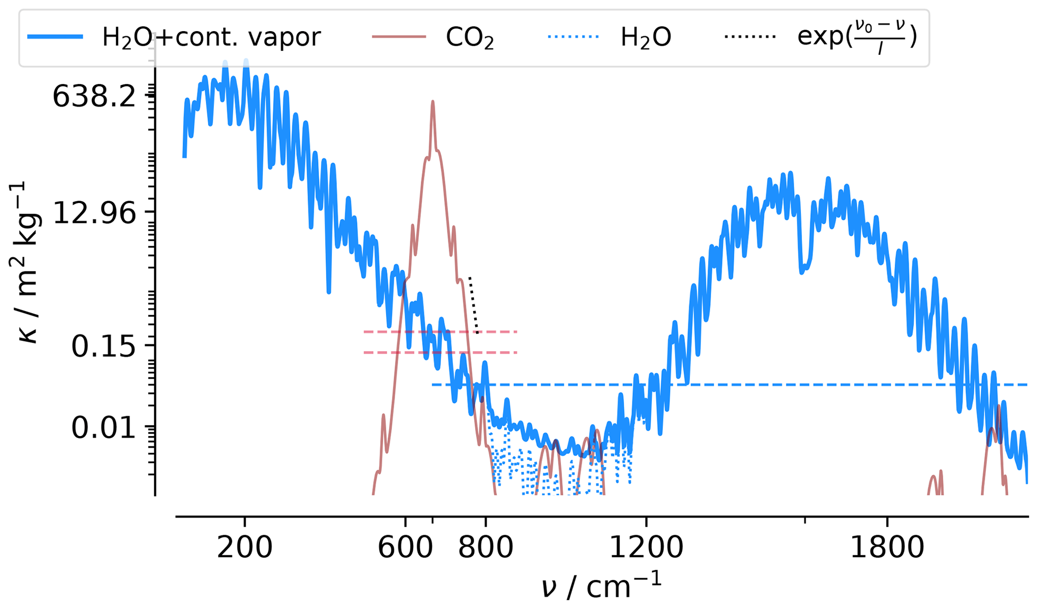
Figure 2 Mass absorption spectrum of H₂O (blue) and CO₂ (red) as a function of wavenumber ν. Spectra are calculated at a wavenumber interval of 0.05 cm⁻¹ for a temperature of 280 K and a pressure of 850 h Pa, and they are smoothed by convolving with a Gaussian (9 cm⁻¹) filter to show the absorption envelope. The black-dotted line (l=10.2 cm⁻¹) is fit to the envelope of the CO₂ band, and the blue-dotted line shows the water vapor absorption in the absence of continuum absorption.

3.1 Spectral masking and the fractional support for the emission response

We introduce the idea of spectral masking as a useful implication of combining Eq. (3) with our classification of emitters. To illustrate the idea, we consider the case where water vapor is the only atmospheric absorber so that $T_{\mathrm{e},\mathrm{y}}=T_{\mathrm{sfc}}$.

Accepting, for the moment, our assertion that the water vapor emission temperature remains invariant, it then follows from Eq. (3) that

$$\begin{array}{}\text{(4)}& \mathit{\delta }{F}_{\mathit{\nu }}=\mathit{\pi }{e}^{-\left({\mathit{\tau }}_{\mathit{\nu },\mathrm{v}}/\mathit{\mu }\right)}\mathit{\delta }{\mathcal{B}}_{\mathit{\nu },\mathrm{sfc}},\end{array}$$

where δℬ_ν,sfc denotes changes from surface emissions at wavenumber ν. Equation (4) can be derived more formally (see, e.g., Eq. 5 in the SI of Koll and Cronin, 2018), which motivates Eq. (3) as a formalization of our ideas instead of the simpler first-to-1 model. From Eq. (4), at wavenumbers where water vapor is optically thick, δF_ν→0. This is what is meant by spectral masking. Put more generally, at wavenumbers where an invariant emitter dominates emissions, it masks the radiative response of underlying sensitive emitters to warming. Jeevanjee et al. (2021a) call this “spectral cancellation of surface feedbacks”. We prefer the term masking because the surface still responds to warming, but, as viewed from space, the response is hidden or masked.

The mass absorption cross-sections of H₂O and CO₂ are presented in Fig. (2). For W≈25 kg m⁻², corresponding to the present-day globally averaged column burden, at wavenumbers where ${\mathit{\kappa }}_{\mathit{\nu },\mathrm{v}}>\mathrm{0.04}$, the atmosphere is considered to be optically thick. This is satisfied over most of the thermal infrared, the exception being wavenumbers between 800 and 1200 cm⁻¹, which define the atmospheric window, emphasizing that it depends on the value of W. Fig. (2) also shows that CO₂, whose column burden C≈6 kg m⁻², is the dominant absorber between 585 and 750 cm⁻¹ and will need to be accounted for in any fuller treatment of the radiative response to warming.

Because W increases exponentially with T_sfc, the atmosphere will become opaque at lower values of κ_ν,v as T_sfc rises, thus reducing its ability to transmit a radiative response to space. We quantify this effect through the introduction of a quantity,

$$\begin{array}{}\text{(5)}& \mathit{\chi }\left(T\right)={\displaystyle \frac{\mathrm{1}}{\mathrm{4}\mathit{\sigma }{T}^{\mathrm{3}}}}\underset{\mathrm{0}}{\overset{\mathrm{\infty }}{\int }}{\displaystyle \frac{\mathrm{d}{F}_{\mathit{\nu }}}{\mathrm{d}T}}\mathrm{d}\mathit{\nu }<\mathrm{1},\end{array}$$

which measures the broadband sensitivity of radiant energy to warming relative to that expected for a black body. Koll and Cronin (2018) introduce the same quantity (their Eq. 4) and call it the average transmission. We prefer to think of χ as the fractional (spectral) support for the radiant response, because this terminology aligns better with the more colorful way of thinking and the first-to-1 model that we keep in the back of our minds.

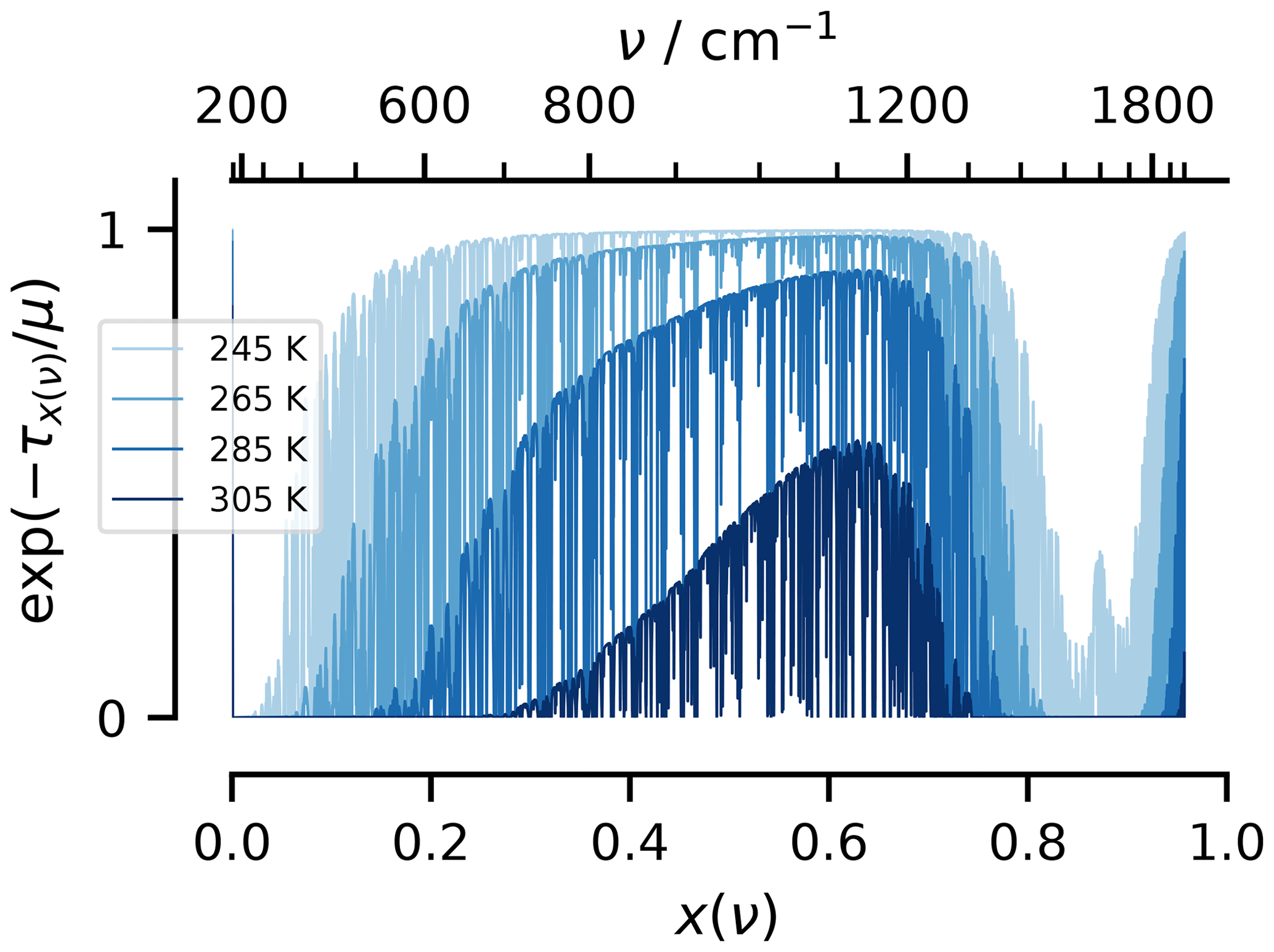
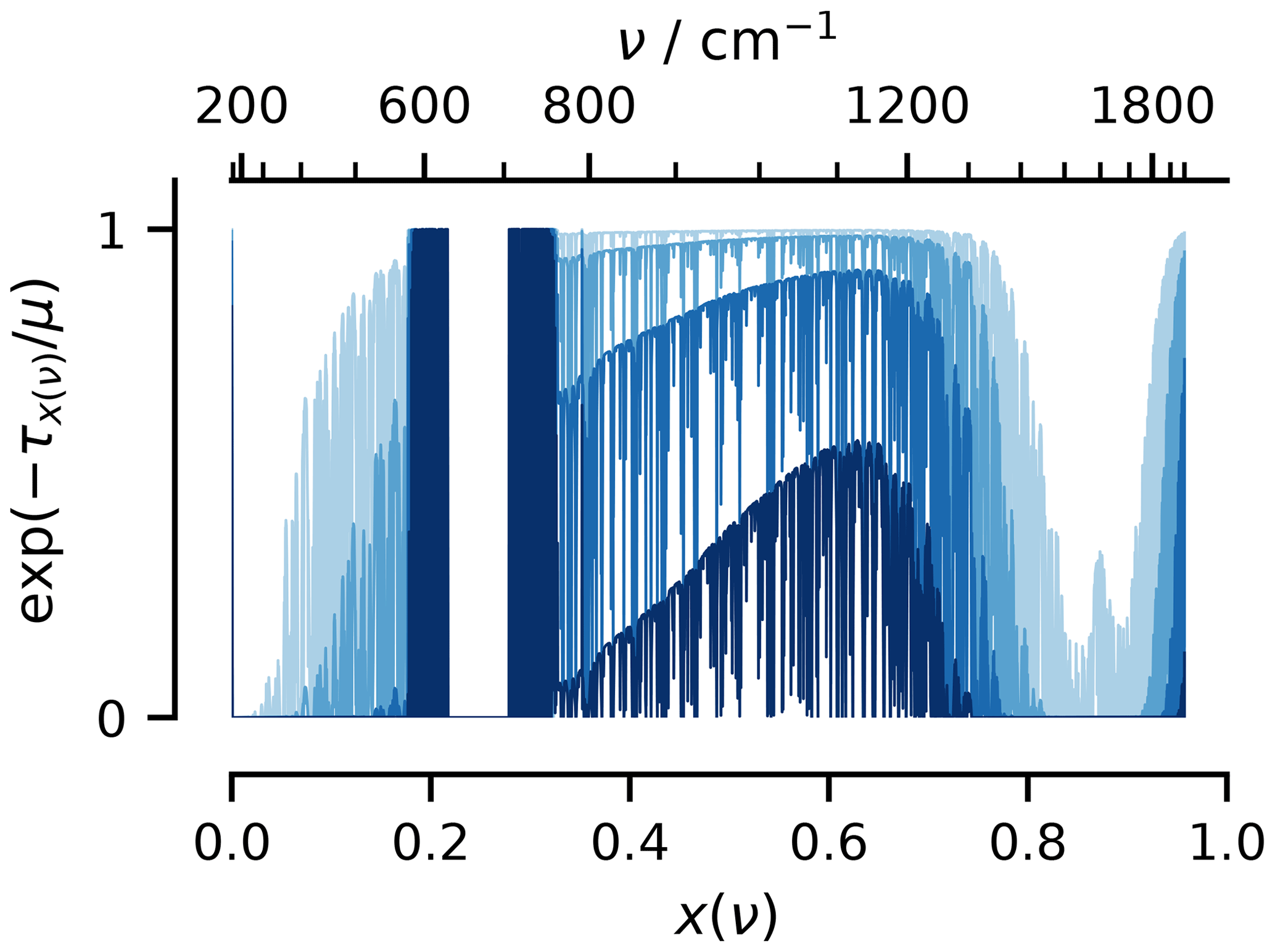
Figure 3 Spectral transmissivity plotted versus the cumulative black-body emission sensitivity, $x=(\mathrm{4}\mathit{\sigma }{T}^{\mathrm{3}}{)}^{-\mathrm{1}}{\int }_{\mathrm{0}}^{\mathit{\nu }}\left(\frac{\mathrm{d}{\mathcal{B}}_{{\mathit{\nu }}^{\prime }}}{\mathrm{d}T}\right)\mathrm{d}{\mathit{\nu }}^{\prime }$. The corresponding wavenumbers are indicated along the upper scale. Line colors darken with T_sfc with W=W_ℛ(T_sfc).

As an example, for the simple case of the water-vapor-only atmosphere δF_ν is given by Eq. (4) and ${\mathit{\tau }}_{\mathit{\nu },\mathrm{v}}\left(T\right)={\mathit{\kappa }}_{\mathit{\nu },\mathrm{v}}W\left(T\right)$, such that

$$\begin{array}{}\text{(6)}& \mathit{\chi }\left(T\right)={\displaystyle \frac{\mathit{\pi }}{\mathrm{4}\mathit{\sigma }{T}^{\mathrm{3}}}}\underset{\mathrm{0}}{\overset{\mathrm{\infty }}{\int }}{e}^{-\frac{{\mathit{\kappa }}_{\mathit{\nu },\mathrm{v}}W\left(T\right)}{\mathit{\mu }}}\left({\displaystyle \frac{\mathrm{d}{\mathcal{B}}_{\mathit{\nu }}}{\mathrm{d}T}}\right)\mathrm{d}\mathit{\nu }.\end{array}$$

Rescaling ν by introducing the coordinate x(ν), such that

$$\begin{array}{}\text{(7)}& \mathrm{d}x={\displaystyle \frac{\mathrm{1}}{\mathrm{4}\mathit{\sigma }{T}^{\mathrm{3}}}}\left({\displaystyle \frac{\mathrm{d}{\mathcal{B}}_{\mathit{\nu }}}{\mathrm{d}T}}\right)\mathrm{d}\mathit{\nu },\end{array}$$

stretches the ν axis so that equally spaced x intervals carry equal amounts of the radiative emission response to warming. In terms of x, $\mathit{\chi }\left(T\right)=\int e^{-{\mathit{\kappa }}_{x,\mathrm{v}}W\left(T\right)/\mathit{\mu }}\mathrm{d}x<\mathrm{1}$ is just the area under the curves in Fig. (3) and shows how an emission response is supported over some subset of x corresponding to wavenumbers where water vapor is optically thin or transparent, i.e., ${\mathit{\kappa }}_{x,\mathrm{v}}\ll \mathit{\mu }/W\left(T\right)$.

For the first-to-1 model, the curves in Fig. (3) would vary between zero and one. Intermediate values emerge both due to spectral averaging and from intermediate optical depths. They highlight the complexity of the line-by-line variability of the spectral transmissivity $e^{-{\mathit{\kappa }}_{x,\mathrm{v}}W\left(T\right)/\mathit{\mu }}$ (which the stroke width used to render the plot is too wide to fully resolve). The effects of the differences between near-line versus continuum (or far-line or dimer) absorption on χ can also be discerned from the way in which the window closes in Fig. (3). The former is associated with a narrowing of the window (region of support) with temperature, while the latter is apparent from weaker support as W becomes large. Continuum emission is more broadband or gray, whereas line absorption, which more nearly results in $e^{-{\mathit{\kappa }}_{x,\mathrm{v}}W/\mathit{\mu }}\in \mathit{\{}\mathrm{0},\mathrm{1}\mathit{\}}$, remains more colorful and better aligns with first-to-1 thinking (i.e., τ_ν,v is either 0 or much larger than 1) and the concept of masking.

3.2 H₂O vapor – an invariant emitter

Simpson's law provides the justification for idealizing water vapor in the troposphere as an invariant emitter and hence for Eq. (4). It states that if the relative humidity ℛ is fixed, W depends only on T. Modulo the effects of pressure broadening on κ_v, this means that τ_ν,v likewise only depends on T, and hence, the emission temperature (effectively where $T({\mathit{\tau }}_{\mathit{\nu },\mathrm{v}}\approx \mathrm{1})$) does not change with warming. This basic idea was developed and used by a number of investigators to study runaway greenhouse atmospheres (Komabayasi, 1967; Ingersoll, 1969; Nakajima et al., 1992) before Ingram (2010) pointed out its earlier articulation by Simpson (1928).

3.2.1 Invariance of W with T with fixed ℛ

The statement that ℛ does not change with warming (Arrhenius, 1896; Simpson, 1928; Manabe and Wetherald, 1967) contains a subtle ambiguity. Is ℛ, as a function of height z, atmospheric pressure P, or temperature T, constant as the surface warms? For a compressible atmosphere, all three cannot be true at once, and which one is meant may have implications for Simpson's law. Assuming that P(T) is bijective through the troposphere, whose top (or lowest pressure) is denoted by the cold-point temperature T_cp, it follows from the definition of W that

$$\begin{array}{}\text{(8)}& W\left(T\right)\approx \underset{T}{\overset{T_{\mathrm{cp}}}{\int }}{P}_{\mathrm{v}}\left(T^{\prime }\right)\left({\displaystyle \frac{R}{g{R}_{\mathrm{v}}}}{\displaystyle \frac{\mathrm{d}\ln P\left(T^{\prime }\right)}{\mathrm{d}{T}^{\prime }}}\right)\mathrm{d}{T}^{\prime },\end{array}$$

with R being the mass-specific gas constant for air and R_v being for water vapor alone. Here, we neglect contributions to W from the stratosphere, an assumption justified both by virtue of the smallness of P_v(T_cp) relative to its values at larger temperatures and because we are mostly interested in $\mathrm{d}W/\mathrm{d}T$, which is constrained by the smallness of the differences in the mass of the stratosphere as the surface warms. Simulations suggests that T_cp is effectively constant across a wide range of conditions characteristic of the tropical atmosphere (Seeley et al., 2019). We introduce it as a parameter, with the value T_cp=194  K taken from radio occultation measurements in the tropics (Tegtmeier et al., 2020), bearing in mind that the same observations show substantially (20 K) larger values in the extra-tropics.

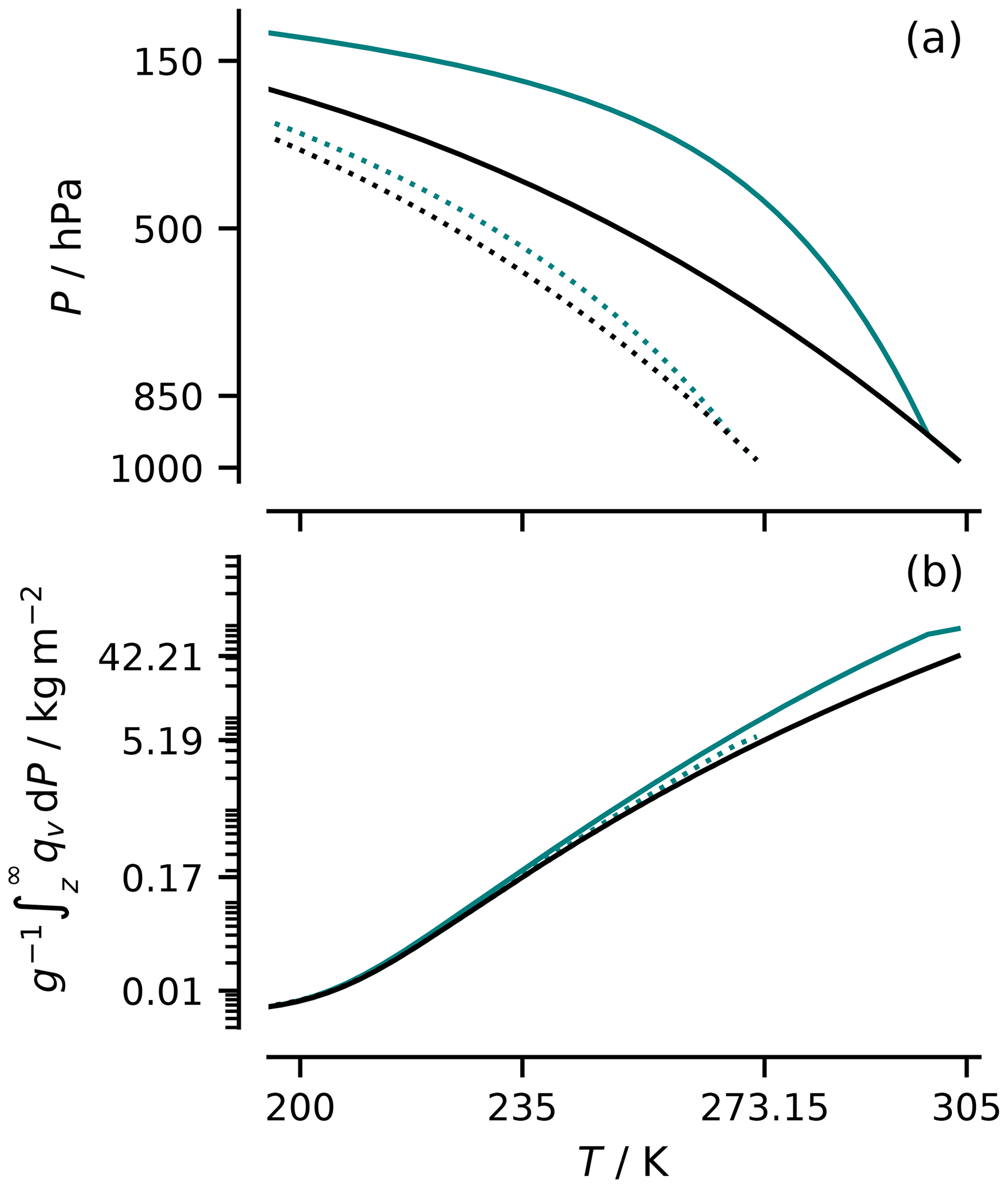
Figure 4 Theoretical temperature profiles and column humidities. Temperature profiles (a) following the formulation of the unsaturated (black) and saturated (teal) moist adiabats in Marquet and Stevens (2022) for two different surface temperatures (as indicated by the tick marks). Column water vapor W(T) between the top of the atmosphere and the height corresponding to the indicated temperature (b).

Equation (8) establishes that W depends only on T as long as both $\mathrm{d}\left(\ln P\right)/\mathrm{d}T$ and ℛ depend only on T. The former (a statement about the lapse rate) is satisfied for an unsaturated adiabat, which describes well the temperature structure of the upper troposphere. In the middle and lower troposphere, the temperature more closely follows the isentropic expansion of saturated air. The impact of allowing $\mathrm{d}\left(\ln P\right)/\mathrm{d}T$ to vary with P as it would following a saturated adiabat is illustrated by Fig. (4). It can be considerable in the lower troposphere. These profiles have been calculated for ℛ=const. Using a C-shaped profile of ℛ, as is more characteristic of the troposphere (Romps, 2014; Bourdin et al., 2021), albeit modified so the anchoring points depend on T, leads to similar conclusions. This then shows the extent to which Simpson's law and many of the idealizations that stem from its use are limited by the variation of ℛ and $\mathrm{d}\left(\ln P\right)/\mathrm{d}T$ with P.

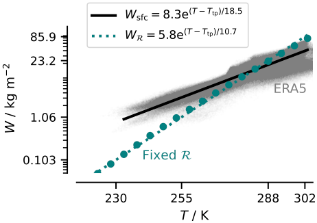
Figure 5 Monthly mean column water vapor W versus monthly mean temperature T for T=T_sfc (gray points) and for the column defined to be between T and T_cp, with fixed ℛ(T) following an idealized C-shaped ℛ(T) profile (filled teal-colored circles). Analytic expressions are fit relative to T_tp=273.16 K, the triple-point temperature, with a crossing point at present-day global temperatures. They are fit to the data by linearly regressing ln (W) binned by T.

3.2.2 Observed variations of W with T_sfc

Over Earth's surface, W varies more weakly with ℛ than it would were ℛ held fixed or if it were allowed to vary with T as it does through the depth of the tropical troposphere. This is shown in Fig. (5), where we compare monthly averaged W as a function of monthly averaged T_sfc, which we denote as W_sfc. For a fixed ℛ, W varies with T following a different relation, which we denote as W_ℛ. Both vary exponentially with T, W_ℛ more sensitively so. This enhanced sensitivity is robust in relation to how ℛ is specified so long as it remains constant with T; C-shaped profiles yield a similar slope. The relative flatness of W_sfc is consistent with ℛ being larger in the cold extra-tropics compared to over the warm sub-tropics, and it is an imprint of the atmospheric circulation.

The implication is that the effect of the circulation is important for describing the spatial distribution of OLR and its scatter (see Fig. 1 in Koll and Cronin, 2018) for a given climate. However, to the extent that the circulation does not change strongly with warming, W_ℛ will better describe W(T). In this case, with global warming, one would expect the cloud of points in Fig. (5) to shift following W_ℛ with global temperature changes. These findings motivate the rather simple choice of ℛ=0.8, chosen so that $W_{\mathcal{R}}(T={\stackrel{\mathrm{‾}}{T}}_{\mathrm{sfc}})$ matches $W_{\mathrm{sfc}}\left({\stackrel{\mathrm{‾}}{T}}_{\mathrm{sfc}}\right)$. A relative humidity of 0.8 is larger than the mean ℛ, as it must be to capture the non-linearity of W(T), whereby $\stackrel{\mathrm{‾}}{W\left(T\right)}>W\left(\stackrel{\mathrm{‾}}{T}\right)$, with an over-bar denoting the global average.

3.3 CO₂ gas – a sensitive and invariant emitter

The heuristic formalized by Eq. (3) also helps understand how CO₂ influences the radiative response to warming. If, in radiative equilibrium, the absorption of radiant energy is independent of T, then the emission must also be independent of T. This is a rough description of the stratosphere and means that, at wavelengths where CO₂ is optically thick in the stratosphere, it behaves like an invariant emitter (see Cronin and Dutta, 2023, for a more thorough discussion of this point). This is not a consequence of Simpson's law, where concentrations adjust to temperature to maintain the same emission. In this case, temperatures adjust to concentrations to maintain the same emission.³

At wavenumbers on the shoulders of its central absorption feature (band), near 600 and 733 cm⁻¹, CO₂ is less absorbing but still absorbing enough to become optically thick within the troposphere. At these wavenumbers, CO₂ behaves like a sensitive emitter. In doing so, it competes with H₂O (more so at wavenumbers on the low-energy side of the absorption band, where H₂O is more absorbing, e.g., Fig. 2) for control of emission to space. At wavenumbers where CO₂ wins the battle by becoming optically thick above the emission height of water vapor, it re-establishes a radiative response to warming that H₂O would have otherwise masked. Where CO₂ emits at heights below the water vapor emission, its radiative response to warming is masked. The lack of concentration gradients in CO₂ complicates the picture as they contribute to a more graduated change in τ_ν,c than in τ_ν,v, which defocuses the emission height and hence the idea of a single or dominant emitter.

Figure 6 As in Fig. 3 but accounting for the effects of CO₂ absorption.

Notwithstanding the difficulties of treating the overlap between CO₂ and water vapor at wavenumbers where both have intermediate optical depths, Eq. (3) helps understand the basic physics of the radiant energy exchange and anticipate effects that gray thinking would obscure. Specifically, to account for CO₂, the dominant emitters in Eq. (3) are chosen based on whether or not an atmospheric absorber is optically thick at a particular value of ν. When τ_ν of one of the absorbers exceeds unity, its emission height and temperature are set to the height where τ_ν=1. When both absorbers are optically thick, the dominant absorber is the first to 1 (lowest emission temperature), and surface emissions (in that case, third to 1) are neglected. By fixing the temperature of the stratosphere to T_cp, we effectively account for stratospheric adjustment and hence for the differentiated response of stratospheric versus tropospheric CO₂ to δT_sfc.

Figure 6 shows the fractional (spectral) support of the response χ calculated using this model. In contrast to Fig. 3, which was calculated for water vapor alone, the spectral support for the radiative response vanishes in the vicinity of the central CO₂ absorption feature at 667 cm⁻¹ and is re-established on its shoulders. Figure 6 highlights the dual role of CO₂ in modulating the radiative response to warming. On the one hand, it masks surface emissions. On the other hand, it re-establishes a radiative response over parts of the spectrum that would otherwise be masked by water vapor. These effects depend on T_sfc. The masking by stratospheric CO₂ becomes more important at colder temperatures, where the stratosphere is more massive and where the troposphere contains less water vapor. The re-establishment of the radiative response on the shoulder of the CO₂ absorption band becomes more prominent at larger T_sfc and is essential for maintaining some support for the radiative response at very warm temperatures. On balance, the presence of CO₂ moderates the dependence of χ on temperature (see Kluft et al., 2021; Seeley and Jeevanjee, 2021)

4 Spectral masking and the clear-sky climate sensitivity

In this section, we apply our heuristic to help understand the radiative response to both warming and to forcing – the two ingredients of the clear-sky climate sensitivity. We show that Eq. (3) not only captures the conceptual content of this recent literature but also presents a quantitatively accurate prediction of the clear-sky sensitivity. This sets the basis for understanding cloud effects in Sect. 5. There, we show how clouds modify the clear-sky response in different ways, with a net effect that does not appear to differ substantially from zero. This establishes the expression for the clear-sky climate sensitivity as a useful estimate of the all-sky sensitivity.

4.1 Radiative response to warming

From our understanding of the temperature influence on the emission of thermal radiation, for small changes in T_sfc, we expect

$$\begin{array}{}\text{(9)}& \mathit{\delta }F=\mathit{\lambda }\mathit{\delta }{T}_{\mathrm{sfc}},\end{array}$$

which introduces the proportionality constant λ as the radiative response parameter. It is closely related to the radiative feedback parameter, which is often denoted by the same symbol using the same expression, modulo a change in the sign convention to allow an increase in F with T to be associated with λ<0, as expected for the net feedback in a stable system. In what follows, we decompose λ into a part that comes from changes in longwave and shortwave radiant energy transfer, such that $\mathit{\lambda }={\mathit{\lambda }}^{\left(\mathrm{lw}\right)}+{\mathit{\lambda }}^{\left(\mathrm{sw}\right)}$.

In clear skies, the longwave radiative response to a change in T_sfc, as predicted by Eq. (3) with the first-to-1 approximation, is given by

$$\begin{array}{}\text{(10)}& \mathrm{\Lambda }\left(T\right)\equiv \mathit{\pi }\int e^{-({\mathit{\tau }}_{\mathit{\nu },\mathrm{v}}/\mathit{\mu })}\left({\displaystyle \frac{\mathrm{d}{\mathcal{B}}_{\mathit{\nu }}}{\mathrm{d}T}}\right)\mathrm{d}\mathit{\nu }=\mathit{\chi }\left(T\right)\mathrm{4}\mathit{\sigma }{T}^{\mathrm{3}},\end{array}$$

where we distinguish the radiative response estimated heuristically, which we denote with Λ, from the true value of the clear-sky radiative response, which we denote with ${\mathit{\lambda }}_{\mathrm{cs}}^{\left(\mathrm{lw}\right)}$. For the case of a pure-water-vapor atmosphere, and modulo ambiguity in how W is defined to vary with T, Eq. (10) is identical to Eq. (3) in Koll and Cronin (2018). It yields the expectation that

$$\begin{array}{}\text{(11)}& {\mathit{\lambda }}_{\mathrm{cs}}^{\left(\mathrm{lw}\right)}\approx \mathrm{\Lambda }\left(T_{\mathrm{sfc}}\right)=\mathit{\chi }\left(T_{\mathrm{sfc}}\right)\mathrm{4}\mathit{\sigma }{T}_{\mathrm{sfc}}^{\mathrm{3}}.\end{array}$$

For T_sfc=288  K and ℛ=0.8, Λ=1.9 Wm⁻² K⁻¹ (Fig. 7), which is indistinguishable from the McKim et al. (2021) estimate for ${\mathit{\lambda }}_{\mathrm{cs}}^{\left(\mathrm{lw}\right)}$ under similar conditions. The estimate of Kluft et al. (2019) is slightly larger at ${\mathit{\lambda }}_{\mathrm{cs}}^{\left(\mathrm{lw}\right)}\approx \mathrm{2.3}$ Wm⁻² K⁻¹, but this is consistent with their calculations having been based on a much drier atmosphere. Figure 7 demonstrates that Λ also captures the sensitivity of ${\mathit{\lambda }}_{\mathrm{cs}}^{\left(\mathrm{lw}\right)}$ to temperature, humidity, and the presence of CO₂, all forms of state dependence that have been identified and explored in a number of recent studies (Koll and Cronin, 2018; Bourdin et al., 2021; McKim et al., 2021; Kluft et al., 2021; Seeley et al., 2019).

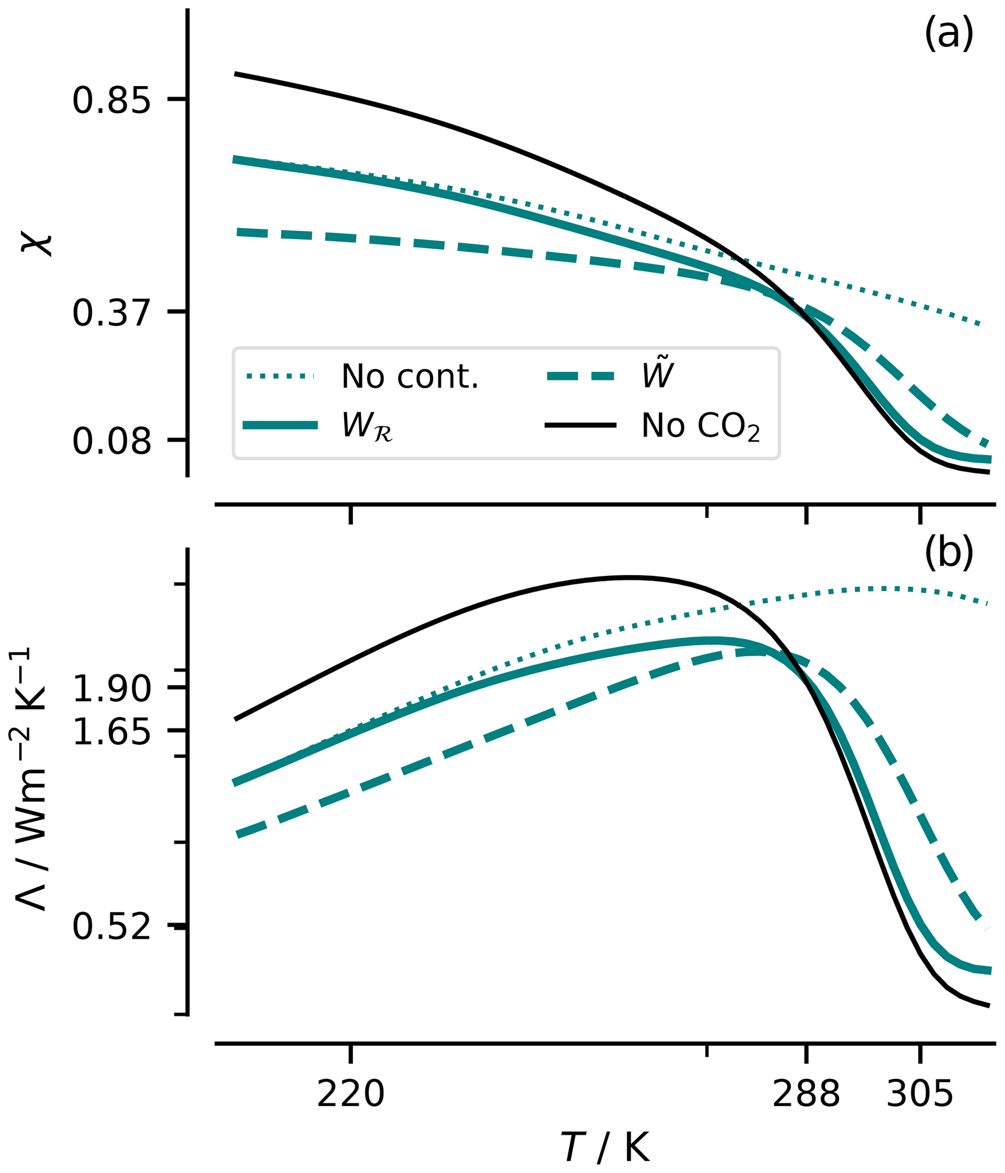
Figure 7 Variation of the support χ(T) (a) and the radiative response to warming Λ with T (b) (minor y axis ticks every 0.5) for different models of W(T). Solid lines show calculations with the inclusion of continuum absorption; the dotted line, for reference, shows the response in the absence of this absorption.

The temperature sensitivity of Λ is interesting in its own right as it explains a state dependence of the climate sensitivity (see also McKim et al., 2021); here, it is also highlighted because it will influence interpretations of cloud effects on the radiative response to warming. From Fig. 7, three temperature regimes can be identified: a cold, T<275 K, “Budyko” regime where Λ increases only slightly ($\mathrm{d}\mathrm{\Lambda }/\mathrm{d}T\approx \mathrm{0.004}$ Wm⁻² K⁻²) and can hence be well approximated as constant, and a warm regime, $\mathrm{285}\mathrm{K}<T<\mathrm{305}\mathrm{K}$, over which the radiative response to warming reduces sharply ($\mathrm{d}\mathrm{\Lambda }/\mathrm{d}T\approx -\mathrm{0.08}$ Wm⁻² K⁻²) with temperature. This is due to closing the atmospheric window due to continuum absorption from water vapor (compare the solid and dotted lines for χ in Fig. 7), and Λ is thus sensitive to the humidity model W_ℛ versus W_sfc (see also McKim et al., 2021, on this point). A third regime emerges at very warm temperatures, T>305 K. Here, Λ is roughly constant but small (Λ≈0.25 Wm⁻² K⁻¹). In this, regime CO₂ plays an important role in maintaining a radiative response (compare solid teal and black lines in Fig. 7) in an atmosphere that is optically thick in water vapor across the thermal infrared (Kluft et al., 2021; Seeley et al., 2019).

The moderating effects of CO₂ on the temperature dependence of Λ reduce its maximum value from 2.55 to 2.17 Wm⁻² K⁻¹ and increase its minimum value from 0.05 to 0.26 Wm⁻² K⁻¹. The former effect arises from spectral masking at wavenumbers where CO₂ is optically thick within the stratosphere and is more important in cold and dry atmospheres where surface emissions would otherwise dominate. The latter effect comes from CO₂ wing absorption reclaiming spectral emissions from water vapor at warm temperatures (Fig. 6). The moderating effect of CO₂ on Λ is somewhat smaller than the warm-regime limit of ${\mathit{\lambda }}_{\mathrm{cs}}^{\left(\mathrm{lw}\right)}\approx \mathrm{1}$ Wm⁻² K⁻¹, as estimated by Kluft et al. (2021) and McKim et al. (2021). Some of the difference can be explained by the use of an unrealistically cold stratosphere in those studies – decreasing T_cp to 150 K increases the asymptotic value of Λ to 0.44 Wm⁻² K⁻¹. The remaining difference likely reflects the crude treatment of emissions at intermediate optical depths by our model.

To the extent that ${\mathit{\lambda }}_{\mathrm{cs}}^{\left(\mathrm{lw}\right)}$ can be usefully approximated by Λ(T_sfc), it demonstrates that this response is something that is quite easy to understand and, given knowledge of the H₂O and CO₂ absorption spectra, to quantify. Moreover, because the dual effects of CO₂ appear to approximately compensate one another at Earth-like temperatures (see Fig. 7), Λ≈Λ_v. This indicates that the reduction in ${\mathit{\lambda }}_{\mathrm{cs}}^{\left(\mathrm{lw}\right)}$ from what would be expected from a black body largely measures how effective water vapor is at controlling emission to space and thereby masking the spectral response of emissions to surface warming, an idea that Ingram (2010) seems to have been the first to appreciate. It also explains why simply approximating

$$\begin{array}{}\text{(12)}& \mathrm{\Lambda }\approx \mathit{\pi }\underset{\mathrm{800}}{\overset{\mathrm{1200}}{\int }}\left({\displaystyle \frac{\mathrm{d}{\mathcal{B}}_{\mathit{\nu }}}{\mathrm{d}T}}\right)\mathrm{d}\mathit{\nu },\end{array}$$

as proposed by Colman and Soden (2021) and as might be justified by the first-to-1 model, provides such a reasonable estimate of ${\mathit{\lambda }}_{\mathrm{cs}}^{\left(\mathrm{lw}\right)}$.

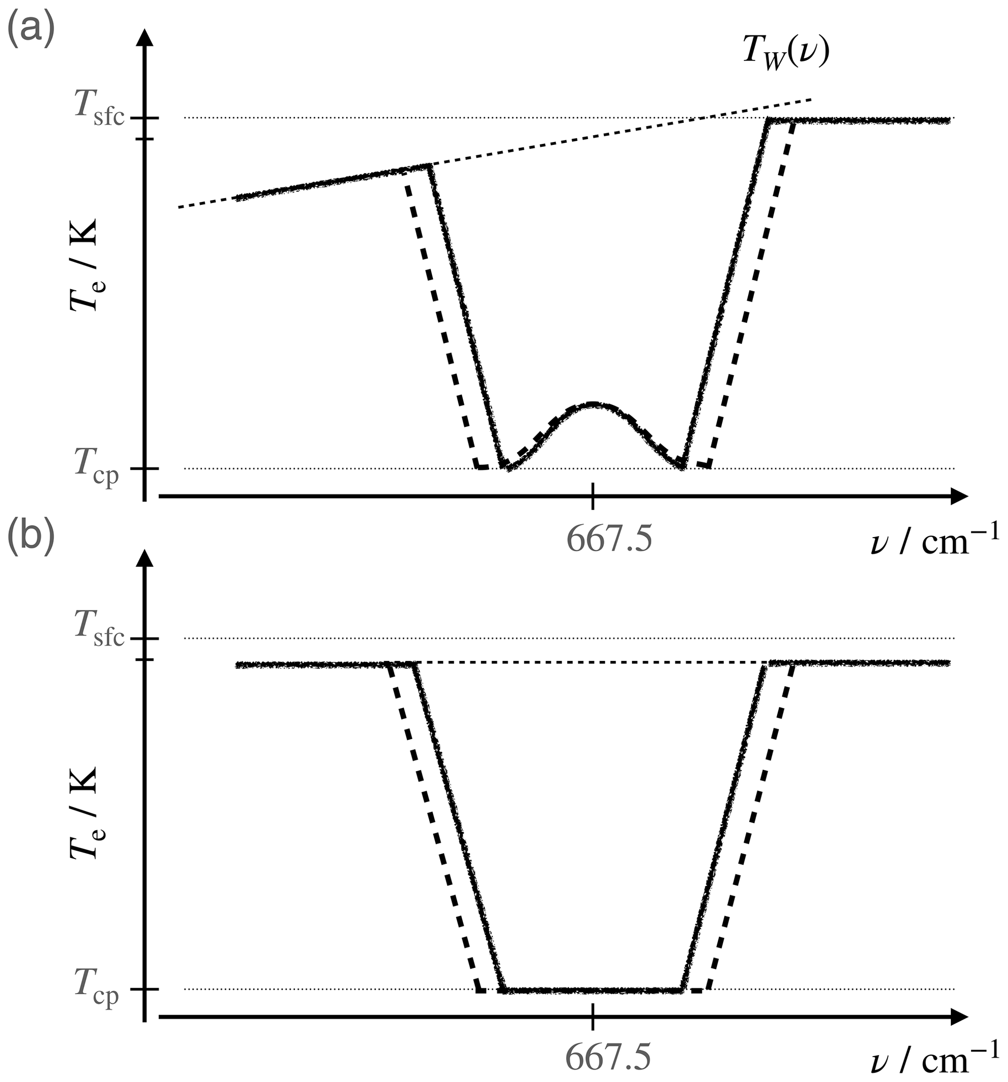
Figure 8 Schematic showing how CO₂ absorption is conceptualized (a) and modeled (calculated) (b). In (a) stratospheric adjustment is conceptualized as maintaining stratospheric emissions near the line center at the same temperature. In (b) an isothermal stratosphere (at T=T_cp) models the invariance of CO₂ emissions in the central part of the absorption band, and the background water vapor emission is assumed to be constant across the band, with its value at the line center.

4.2 Clear-sky radiative response to (CO₂) forcing

Application of Eq. (3) yields a model of CO₂ forcing similar to that first proposed by Wilson and Gea-Banacloche (2012) and developed later, in more detail, by Jeevanjee et al. (2021b). The starting point is to describe the irradiance as a function of the CO₂ burden C, its spectral mass absorption coefficient κ_ν,c, and the limiting temperatures T_cp and T_⋆, such that

$$\begin{array}{}\text{(13)}& \begin{array}{rl}F\left(C\right)& =\mathit{\pi }\underset{\mathrm{0}}{\overset{\mathrm{\infty }}{\int }}\left[e^{-C{\mathit{\kappa }}_{\mathit{\nu },\mathrm{c}}/\mathit{\mu }}{\mathcal{B}}_{\mathit{\nu }}\right(T_{\star })\\ & +\left(\mathrm{1}-e^{-C{\mathit{\kappa }}_{\mathit{\nu },\mathrm{c}}/\mathit{\mu }}\right){\mathcal{B}}_{\mathit{\nu }}\left(T_{\mathrm{cp}}\right)]\mathrm{d}\mathit{\nu },\end{array}\end{array}$$

with $T_{\star }=min(T_{\mathrm{sfc}},T_{*})$ where $W_{\mathcal{R}}\left(T_{*}\right)={\mathit{\kappa }}_{\mathit{\nu },\mathrm{v}}^{-\mathrm{1}}$. This defines T_⋆ as the temperature at which the W, distributed with T_sfc following W_ℛ, would attain an optical thickness of 1 or T_sfc, whichever is smaller. Through its dependence on κ_ν,v, it will vary with ν. The choice of a fixed stratospheric CO₂ emission temperature set to the cold point (Fig. 8b) provides a simple way to account for stratospheric adjustment (Hansen et al., 1997) by ensuring that the emission temperature of stratospheric CO₂ remains invariant. As such, it anticipates our interest in the radiative response to changing CO₂, i.e., the forcing.

An N-fold increase in the burden gives rise to ℱ, given by the change in the irradiance (Eq. 13) at the new burden; in clear skies, this becomes

$$\begin{array}{}\text{(14)}& \begin{array}{rl}{\mathcal{F}}_{\mathrm{cs}}\left(N\right)& =F\left(NC\right)-F\left(C\right)\\ & =\mathit{\pi }\underset{\mathrm{0}}{\overset{\mathrm{\infty }}{\int }}\left(e^{-C{\mathit{\kappa }}_{\mathit{\nu },\mathrm{c}}/\mathit{\mu }}-e^{-NC{\mathit{\kappa }}_{\mathit{\nu },\mathrm{c}}/\mathit{\mu }}\right)\\ & \left[{\mathcal{B}}_{\mathit{\nu }}\left(T_{\star }\right)-{\mathcal{B}}_{\mathit{\nu }}\left(T_{\mathrm{cp}}\right)\right]\mathrm{d}\mathit{\nu }.\end{array}\end{array}$$

As climate sensitivity is usually referred to as the temperature response to a doubling of atmospheric CO₂, in the remainder of the paper, we equate ℱ_cs with ℱ_cs(2). With T_cp=200 K ranging from 194 to 204 K (Tegtmeier et al., 2020), ℱ_cs varies from 4.55 to 4.22 Wm⁻². These values compare favorably with estimates of the adjusted clear-sky flux in the literature, which range from 4.3 to 4.9 Wm⁻² (Kluft et al., 2019, 2021). The model is not only qualitatively informative; it also has quantitative fidelity, as demonstrated by is ability to capture the sensitivities to various quantities seen in more complex calculations, e.g., as in Jeevanjee et al. (2021b).

Following Wilson and Gea-Banacloche (2012) and subsequent studies (e.g., Seeley, 2018; Jeevanjee et al., 2021b), two approximations make it possible to cast Eq. (14) into an even simpler form. The first is to replace the Planck source function with its band-averaged or band-centered values. This is justified because the difference between the CO₂ transmissivities vanishes for ${\mathit{\tau }}_{\mathit{\nu },\mathrm{c}}\ll \mathrm{1}$ and for ${\mathit{\tau }}_{\mathit{\nu },\mathrm{c}}\gg \mathrm{1}$ so that ℬ_ν only contributes to the integral in the vicinity of ν_c. This allows it to be approximated by its central value and for T_⋆ to be approximated by a band-averaged (567.5 to 767.5 cm⁻¹) value:

$$\stackrel{\mathrm{‾}}{T_{\star }}\equiv {\displaystyle \frac{\mathrm{1}}{\mathrm{200}{\mathrm{cm}}^{-\mathrm{1}}}}\underset{\mathrm{567.5}}{\overset{\mathrm{767.5}}{\int }}{T}_{\star }\mathrm{d}\mathit{\nu }\approx \mathrm{282.13}\mathrm{K},$$

where T_⋆ is defined as previously described. The second approximation is justified graphically in Fig. 2, which shows that the envelope of the CO₂ absorption spectrum falls off exponentially with ν as $\mathit{\alpha }{e}^{-\Vert \mathit{\nu }-{\mathit{\nu }}_{\mathrm{c}}\Vert /l}$. This implies that, for a CO₂ burden of C, ${\mathit{\tau }}_{\mathit{\nu },\mathrm{c}}>\mathrm{1}$ for ${\mathit{\nu }}_c-l\ln \left(\mathit{\alpha }C\right)<\mathit{\nu }<{\mathit{\nu }}_c+l\ln \left(\mathit{\alpha }C\right).$ It follows that, for a burden of NC, the atmosphere becomes optically thick for the larger interval – larger by the amount 2lln (N). With these simplifications, Eq. (14) is simplified to

$$\begin{array}{}\text{(15)}& {\mathcal{F}}_{\mathrm{cs}}\left(N\right)\approx \mathrm{2}\mathit{\pi }l\ln N\left[{\mathcal{B}}_{{\mathit{\nu }}_{\mathrm{c}}}(min(\stackrel{\mathrm{‾}}{T_{\star }},T_{\mathrm{sfc}}\left)\right)-{\mathcal{B}}_{{\mathit{\nu }}_{\mathrm{c}}}\left(T_{\mathrm{cp}}\right)\right].\end{array}$$

For the same range of T_cp (194 to 204 K), ℱ_cs varies from 4.3 to 4.0 Wm⁻², comparable to estimates from the direct integration of Eq. (14).

4.3 Clear-sky climate sensitivity

Dividing the estimate of the forcing from Eq. (14) by the radiative response from Eq. (10) gives an expression for the clear-sky climate sensitivity 𝒮_cs:

$$\begin{array}{}\text{(16)}& {\mathcal{S}}_{\mathrm{cs}}={\displaystyle \frac{{\int }_{\mathrm{0}}^{\mathrm{\infty }}\left(e^{\frac{-{\mathit{\kappa }}_{\mathit{\nu },\mathrm{c}}C}{\mathit{\mu }}}-e^{\frac{-\mathrm{2}{\mathit{\kappa }}_{\mathit{\nu },\mathrm{c}}C}{\mathit{\mu }}}\right)\left[{\mathcal{B}}_{\mathit{\nu }}\left(T_{\star }\right)-{\mathcal{B}}_{\mathit{\nu }}\left(T_{\mathrm{cp}}\right)\right]\mathrm{d}\mathit{\nu }}{{\int }_{\mathrm{0}}^{\mathrm{\infty }}{e}^{\frac{-{\mathit{\kappa }}_{\mathit{\nu },\mathrm{v}}W}{\mathit{\mu }}}\left(\frac{\mathrm{d}{\mathcal{B}}_{\mathit{\nu }}}{\mathrm{d}T}\right)\mathrm{d}\mathit{\nu }}}=\mathrm{2.3}\mathrm{K},\end{array}$$

where T_cp is taken as the average across the stated range, and the net effect of CO₂ on the radiative response to surface warming is assumed to be negligible. The additional simplifications of Eq. (15) for forcing and Eq. (12) for the radiative response yield a simpler expression in that it no longer depends explicitly on the absorption spectra of CO₂ and H₂O. With these approximations,

$$\begin{array}{}\text{(17)}& {\mathcal{S}}_{\mathrm{cs}}\approx {\displaystyle \frac{{\mathcal{B}}_{{\mathit{\nu }}_{\mathrm{c}}}(min(\stackrel{\mathrm{‾}}{T_{\star }},T_{\mathrm{sfc}}\left)\right)-{\mathcal{B}}_{{\mathit{\nu }}_{\mathrm{c}}}\left(T_{\mathrm{cp}}\right)}{\mathrm{2}\mathit{\sigma }{\int }_{\mathrm{800}}^{\mathrm{1200}}\left(\frac{\mathrm{d}{\mathcal{B}}_{\mathit{\nu }}}{\mathrm{d}T}\right)\mathrm{d}\mathit{\nu }}}l\ln \mathrm{2}=\mathrm{2.4}\mathrm{K}.\end{array}$$

By virtue of assuming a fixed window, Eq. (17) will not, however, generalize as well as Eq. (16) to warmer temperatures.

As a comparison, for radiative convective equilibrium, Kluft et al. (2019) estimate 𝒮_cs=2.1 K, albeit for a drier atmosphere. The ability to derive Eq. (16) from the simple heuristic and its interpretation and/or simplification in the form of Eq. (17) illustrate how the value of the clear-sky climate sensitivity and its dependence on quantities like surface and tropopause temperature (T_cp) are quite easy to understand and predict. This understanding, as we show next, provides a different, and we believe better, basis for quantifying the effect of clouds.

5 Inferences for Earth's atmosphere and estimates of the all-sky climate sensitivity 𝒮

In this section, we explore how our more colorful way of thinking helps us understand how clouds influence the all-sky climate sensitivity 𝒮. Equation (9) provides the basis for defining the climate sensitivity 𝒮 as the temperature response to a doubling of atmospheric CO₂, such that

$$\begin{array}{}\text{(18)}& \mathcal{S}={\displaystyle \frac{\mathcal{F}}{{\mathit{\lambda }}^{\left(\mathrm{lw}\right)}+{\mathit{\lambda }}^{\left(\mathrm{sw}\right)}}}.\end{array}$$

For a fixed planetary albedo⁴, λ^(sw)=0. In this case, $\mathcal{S}=\mathcal{F}/{\mathit{\lambda }}^{\left(\mathrm{lw}\right)}\ne {\mathcal{S}}_{\mathrm{cs}}$, which is to say that clouds influence the climate sensitivity through more than their effect on the planetary albedo.

In Sect. 5.1 below, we explore how clouds influence λ^(lw) and ℱ independently of changes in cloud cover. We extend previous work that focused on cloud masking – what Yoshimori et al. (2020) called the cloud climatological effect – to show how changing cloud top temperatures can actually enhance λ^(lw) relative to ${\mathit{\lambda }}_{\mathrm{cs}}^{\left(\mathrm{lw}\right)}$. The impact of these effects is explored with a few examples in Sect. 5.2. In Sect. 5.3, we develop a framework for estimating 𝒮 using estimates of cloud and surface albedo changes from the literature to calculate λ^(sw), and we link this to our understanding of λ^(lw) to develop what we believe to be a more physical framework for understanding how various processes influence 𝒮, including the net effect of clouds.

5.1 The effects of clouds on the climate sensitivity for no changes in albedo

From a radiant energy transfer perspective, one important distinction between clouds and water vapor is that clouds are neither colorful nor necessarily Simpsonian. Their grayness makes them effective in modifying both the clear-sky forcing and the clear-sky radiative response to warming. Some of these effects are well known, but others are only beginning to be appreciated or have been overlooked entirely.

5.1.1 Cloud effects on forcing ℱ

While it is well known that clouds mask the radiative forcing (Myhre et al., 1998), this is often overlooked when taking the measure of the cloud effect on climate sensitivity. For those wavenumbers where, in a cloud-free atmosphere, CO₂ controls the emissions to space, clouds with cloud top pressures lower than the CO₂ emission pressure will wrest control of emissions and mask the changes from changing CO₂ concentrations. Even when cloud top pressures are greater than the CO₂ emission pressure, so long as cloud top temperatures lie below the clear-sky (and CO₂-free) emission temperature T_⋆, (see Eq. 14) clouds will reduce the strength of the CO₂ forcing. Only in the case of clouds capping a surface inversion is it conceivable that they might increase ℱ relative to its clear-sky value.

To quantify the reduction of cloud forcing from clouds, we define the high-cloud fraction to be the effective masking fraction f_h, such that

$$\begin{array}{}\text{(19)}& \mathcal{F}=\left(\mathrm{1}-f_{\mathrm{h}}\right){\mathcal{F}}_{\mathrm{cs}}.\end{array}$$

It implies that, for ℱ_cs=4.9 Wm⁻² (as calculated by Kluft et al., 2019), f_h≈0.25 would result in ℱ=3.7 Wm⁻². To the extent that f_h should be compared to the geometrically high-cloud fraction, this appears to be a reasonable value. It is also consistent with Myhre et al. (1998), who estimate a similar 27 %, reduction in CO₂ forcing due to clouds.

5.1.2 Cloud effects on the longwave radiative response λ^(lw)

When the cloud top emission temperature T_cld does not change with warming, clouds mask window emissions in proportion to their (optically thick) cloud fraction (McKim et al., 2021), which we associate with the total (optically thick) cloud fraction f≈0.6 (from AATSR). This leads to a nearly commensurate reduction in λ^(lw) from its clear-sky value of 1.9 to 0.76 Wm⁻² K⁻¹. We say nearly because of the ability of CO₂ to restore some of the radiative response where its emission height lies above the clouds but below the tropopause. Because all clouds rather than just high clouds contribute to the masking of emissions from the surface, the reduction in the radiative response from cloud masking will be larger than the reduction in the forcing, roughly by a factor of $(\mathrm{1}-f_{\mathrm{h}})/(\mathrm{1}-f)\approx \mathrm{1.875}$. This will increase 𝒮 relative to 𝒮_cs, raising its value to ≈3.6  K.

What seems to have escaped attention is how clouds might restore parts of the spectral response otherwise masked by water vapor. To quantify these competing effects, we model the effects of clouds on λ^(lw) as

$$\begin{array}{}\text{(20)}& \begin{array}{rl}{\mathit{\lambda }}^{\left(\mathrm{lw}\right)}& \approx (\mathrm{1}-f)\mathrm{\Lambda }\left(T_{\mathrm{sfc}}\right)+f{\displaystyle \frac{\mathit{\delta }{T}_{\mathrm{cld}}}{\mathit{\delta }{T}_{\mathrm{sfc}}}}\mathrm{\Lambda }\left(T_{\mathrm{cld}}\right)\\ & =(\mathrm{1}-\mathit{\eta }f)\mathrm{\Lambda }\left(T_{\mathrm{sfc}}\right),\end{array}\end{array}$$

with

$$\begin{array}{}\text{(21)}& \mathit{\eta }=\mathrm{1}-{\displaystyle \frac{\mathit{\delta }{T}_{\mathrm{cld}}}{\mathit{\delta }{T}_{\mathrm{sfc}}}}{\displaystyle \frac{\mathrm{\Lambda }\left(T_{\mathrm{cld}}\right)}{\mathrm{\Lambda }\left(T_{\mathrm{sfc}}\right)}}.\end{array}$$

If δT_cld=0, then η=1, and Eq. (20) describes the masking of the clear-sky response (assuming ${\mathit{\lambda }}_{\mathrm{cs}}^{\left(\mathrm{lw}\right)}\approx \mathrm{\Lambda }\left(T_{\mathrm{sfc}}\right)$) by clouds – as discussed by McKim et al. (2021) and Yoshimori et al. (2020). The emission response across the spectrum as restored by clouds is made manifest by η<1, whereby η<0, implying that an all-sky radiative response greater than that of the clear skies is not precluded.

This demonstrates how the effect of clouds on the longwave radiative response depends on $\frac{\mathit{\delta }{T}_{\mathrm{cld}}}{\mathit{\delta }{T}_{\mathrm{sfc}}}$ through its effect on η. From Fig. 7 we can also infer that, for the same change in cloud-top temperatures, the ability to restore the radiative response will be stronger in the warm regime, where $\mathrm{\Lambda }\left(T_{\mathrm{cld}}\right)/\mathrm{\Lambda }\left(T_{\mathrm{sfc}}\right)>\mathrm{1}$ than in the cold regime.

5.2 Some examples of cloud effects on the fixed albedo climate sensitivity

The above analysis identifies ways in which the amount and distribution of clouds influences estimates of climate sensitivity even if the coverage, albedo, and temperature of the clouds do not change. It also identifies δT_cld as a bit of a joker through its ability to substantially increase or decrease the radiative response. Below, we work through a few examples to illustrate these effects.

5.2.1 High clouds in the wet tropics

In the warm tropical atmosphere, where precipitating convection is embedded in a nearly saturated atmosphere (Bretherton and Peters, 2004), clouds may be especially important for the radiative response to warming. As the window closes, Λ(T_sfc)→0, and there is little (only the CO₂ wing emissions) left for clouds to mask (Stephens et al., 2016). In this case, the first term in Eq. (20) becomes negligible, independent of f; clouds with cold cloud tops will carry the bulk of the radiative response; and its magnitude will be given by the second term, which is proportional to the cloud fraction and the cloud top temperature change. This would provide a radiator for the tropical hothouse, one which, together with wing emission from CO₂ (Kluft et al., 2021; Seeley and Jeevanjee, 2021), prevents the window from completely closing, thereby helping to moderate temperature increases. The degree of moderation will depend on the degree to which cloud top temperature changes are constrained by the radiative cooling in the clear-sky atmosphere, which is still a matter of some debate (Zelinka and Hartmann, 2010, 2011; Bony et al., 2016; Seeley et al., 2019; Hartmann et al., 2022).

5.2.2 Low clouds coupled to surface temperature

In the case that clouds warm with the surface, δT_cld≈δT_sfc, and ${\mathit{\lambda }}^{\left(\mathrm{lw}\right)}\approx \mathrm{\Lambda }\left(T_{\mathrm{sfc}}\right)+f\left[\left(\mathrm{\Lambda }\right(T_{\mathrm{cld}})-\mathrm{\Lambda }(T_{\mathrm{sfc}})\right]$. In the warm regime, Λ decreases with temperature, and because cloud tops are colder than the surface, $\mathrm{\Lambda }\left(T_{\mathrm{cld}}\right)-\mathrm{\Lambda }\left(T_{\mathrm{sfc}}\right)>\mathrm{0}$. Candidate cloud regimes for such behavior would be clouds topping the trade wind layer (Schulz et al., 2021) or clouds in the doldrums. In these cases, one might expect $T_{\mathrm{sfc}}-T_{\mathrm{cld}}\approx$ 7 to 15 K, with surface temperatures increasingly exceeding 300 K. In this situation, from Fig. 7, clouds with tops at 288 K will radiate about 4-fold more energy per degree of warming than would a surface at 305 K. More detailed calculations, e.g., Kluft et al. (2021), suggest a smaller, 2-fold difference but suffer from simplifications to the stratosphere, suggesting that the real answer lies somewhere in between. In either case, the effect appears to be appreciable and illustrates how shallow boundary layer clouds, even small ones that cover most of the tropical oceans but generally go unnoticed (Mieslinger et al., 2022; Konsta et al., 2022), may help stabilize the climate. Over the cold extra-tropics, where Λ increases with temperature, clouds (which emit at temperatures colder than the surface) have the opposite effect.

Measurements in the window region could help answer how much clouds warm with surface temperatures; here, we ask how much they would have to warm to counter their additional masking effect relative to that of the forcing. This situation would be met with λ^(lw)≈f_hΛ. From Eq. (20), with$\mathit{\eta }=f_{\mathrm{h}}/f$, this is satisfied for

$$\begin{array}{}\text{(22)}& \mathit{\delta }{T}_{\mathrm{cld}}=\mathit{\delta }{T}_{\mathrm{sfc}}\left(\mathrm{1}-{\displaystyle \frac{f_{\mathrm{h}}}{f}}\right){\displaystyle \frac{\mathrm{\Lambda }\left(T_{\mathrm{sfc}}\right)}{\mathrm{\Lambda }\left(T_{\mathrm{cld}}\right)}}\approx {\displaystyle \frac{\mathrm{1}}{\mathrm{2}}}\mathit{\delta }{T}_{\mathrm{sfc}},\end{array}$$

for f_h=0.25, f=0.6, and $\mathrm{\Lambda }\left(T_{\mathrm{sfc}}\right)/\mathrm{\Lambda }\left(T_{\mathrm{cld}}\right)$ slightly less than 1 (from Fig. 7, corresponding to the warm regime).

5.2.3 Multi-layer clouds

This analysis can be generalized to clouds distributed over multiple layers by working one's way down through the successive contribution of layers of non-overlapped clouds:

$$\begin{array}{}\text{(23)}& {\mathit{\lambda }}^{\left(\mathrm{lw}\right)}=\mathrm{\Lambda }\left(T_{\mathrm{sfc}}\right)\left[\mathrm{1}-\sum _i{\mathit{\eta }}_i{f}_i^{\prime }\right],\end{array}$$

where $f_i^{\prime }$ denotes the cloud fraction for layer i (increasing downward) that is not geographically masked by clouds at layers j<i, and η_i indexes changes in cloud top temperature.

5.2.4 Clouds and the clear-sky polar-amplification paradox

From the point of view of the radiant transfer of energy in the thermal infrared, the idea that the polar latitudes should warm disproportionately is a curious one as the radiative forcing from a doubling of atmospheric CO₂ is proportional to T_sfc−T_cp, which is much smaller in the polar regions, and the radiative response to warming is, by virtue of the absence of water vapor to mask surface emissions, particularly large. Put differently, from our understanding of 𝒮_cs, for a fixed albedo and in the absence of lateral energy transport, the tropics should warm substantially more than the poles as CO₂ increases. This is less of a paradox when one considers the differences between the poles and the tropics, whether it be by virtue of surface albedo changes or the decoupling of the polar surface from the polar atmosphere. Here we point out the potential for clouds to also cause a differentiated response of the cold poles versus the warm tropics to warming.

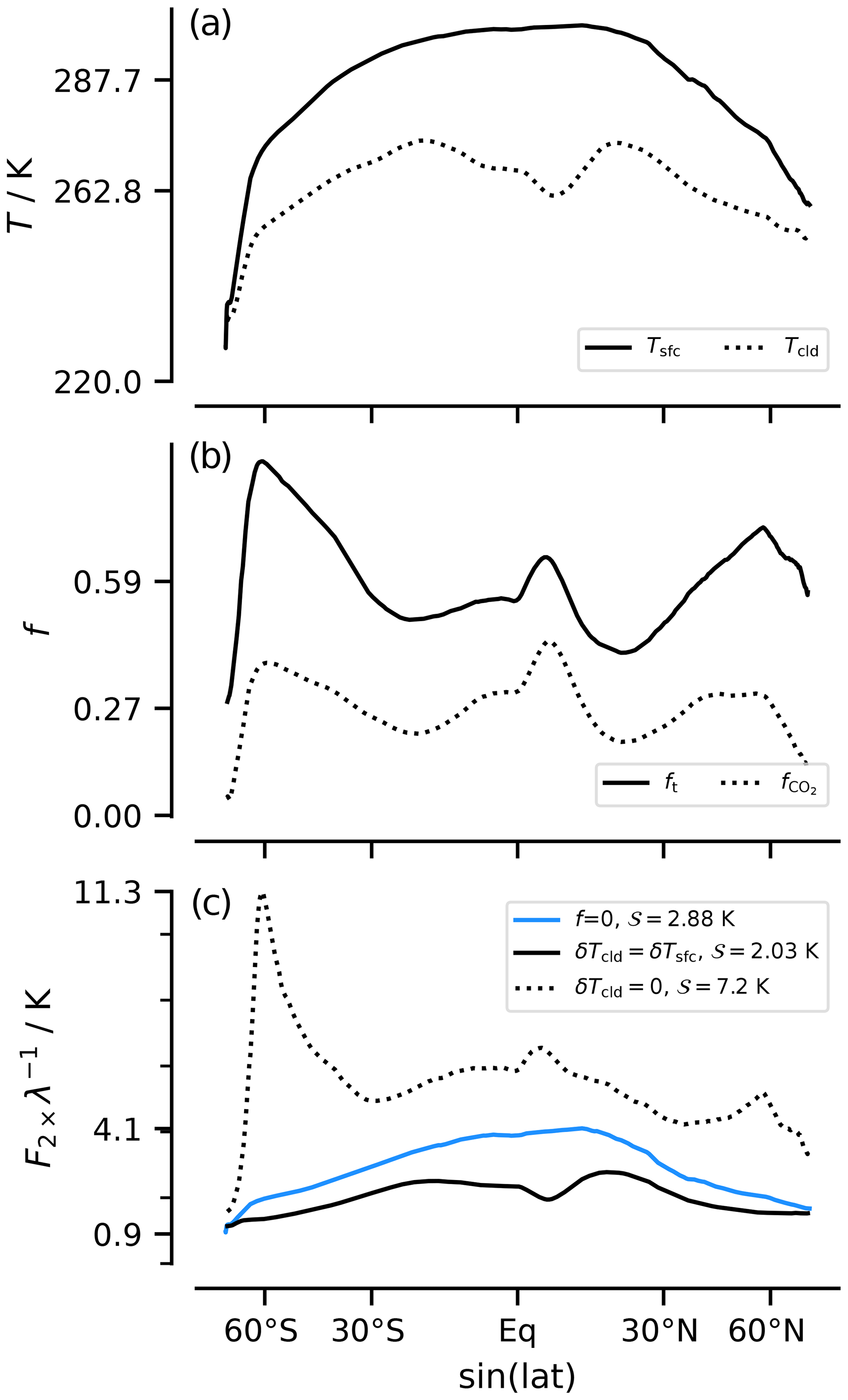
Figure 9 Latitudinal distribution of T_sfc and T_cld (a), total cloud fraction f and the fraction assumed to mask CO₂ forcing ℱ (b), and the ratio of the forcing ℱ to the radiative response to warming λ^(lw) for different assumptions about clouds (c).

To do so, we compare estimates of the local sensitivity $\mathcal{F}/{\mathit{\lambda }}^{\left(\mathrm{lw}\right)}$. We calculate λ^(lw) following Eq. (20), using W_sfc(T_sfc) to calculate Λ(T_sfc) and W_ℛ to calculate Λ(T_cld). This is an admittedly crude way to treat the variation of W with height at different geographic regions, but using W_sfc for the cloud term as well does not change the answer appreciably. The albedo is kept constant, and clouds are represented using three bounding cases: (i) f=0, which renders clouds as transparent; (ii) δT_cld=δT_sfc, whereby clouds warm with the surface; and (iii) δT_cld=0, what one might call Simpsonian clouds. To calculate the forcing ℱ requires an estimate of the fraction of the forcing f_h masked by clouds at different latitudes. We estimate this quite crudely based on the fractional decrease of the cloud top temperature (as taken from the AATSR data) relative to the temperature change through the troposphere as a whole:

$$\begin{array}{}\text{(24)}& f_{\mathrm{h}}=\mathrm{1.9}\left({\displaystyle \frac{T_{\mathrm{sfc}}-T_{\mathrm{cld}}}{T_{\mathrm{sfc}}-T_{\mathrm{cp}}}}\right)f.\end{array}$$

The pre-factor (1.9) is introduced and set so that $\stackrel{\mathrm{‾}}{\mathcal{F}}$ matches the estimate of 3.7 Wm⁻² of more detailed calculations. Because 𝒮 is defined as a global (or statistical) quantity, it is estimated as $\stackrel{\mathrm{‾}}{\mathcal{F}}/\stackrel{\mathrm{‾}}{{\mathit{\lambda }}^{\left(\mathrm{lw}\right)}}$.

The results of these calculations are shown in Fig. 9. For case (i), with transparent clouds where f=0, values of $\mathcal{F}/{\mathit{\lambda }}^{\left(\mathrm{lw}\right)}$ vary with latitude, from a low value (0.9 K) over the South Pole to a high value (4.1 K) over the Intertropical Convergence Zone region just north of the Equator, thereby illustrating what we call the polar-amplification paradox. For this case, 𝒮=2.9 K, which is slightly larger than the clear-sky estimates obtained previously using global mean quantities. For case (ii) with warming clouds (δT_cld=δT_sfc), 𝒮=2.0  K, with reductions being most pronounced in the tropics, where additional emissions from clouds occur in an atmosphere that is less masked by water vapor. Given the idea that high clouds maintain a fixed temperature, this case might seem extreme; then again, warming along the moist adiabat is upward amplified so that the case of fixed cloud height actually implies δT_cld>δT_sfc, which can be thought of as a form of lapse rate feedback. For case (iii) with δT_cld=0, clouds mask the radiative response, and 𝒮 increases considerably, inverting its geographic structure to be more poleward amplified. Hence, high clouds that do not warm with the surface greatly sensitize the poles to increasing CO₂.

5.3 All-sky climate sensitivity

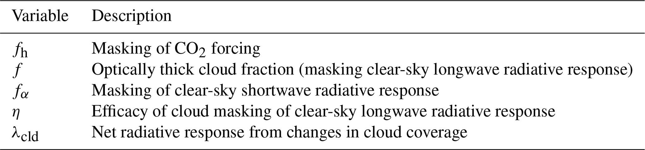
Returning to Eq. (9) and introducing λ_cld to represent the (long- and shortwave) radiative response to changes in the coverage (or albedo) of clouds and $(\mathrm{1}-f_{\mathit{\alpha }}){\mathit{\lambda }}_{\mathrm{cs}}^{\left(\mathrm{sw}\right)}$ to represent the all-sky changes in shortwave radiation with warming,

$$\begin{array}{}\text{(25)}& \mathcal{S}={\displaystyle \frac{(\mathrm{1}-f_{\mathrm{h}}){\mathcal{F}}_{\mathrm{cs}}}{(\mathrm{1}-\mathit{\eta }f){\mathit{\lambda }}_{\mathrm{cs}}^{\left(\mathrm{lw}\right)}-{\mathit{\lambda }}_{\mathrm{cld}}-(\mathrm{1}-f_{\mathit{\alpha }}){\mathit{\lambda }}_{\mathrm{cs}}^{\left(\mathrm{sw}\right)}}}.\end{array}$$

By writing the surface albedo changes in terms of their clear-sky value ${\mathit{\lambda }}_{\mathrm{cs}}^{\left(\mathrm{sw}\right)}$, we account for cloud masking through f_α so that Eq. (25) explicitly accounts for the varied cloud effects on climate sensitivity (see also Table 2). The contribution of cloud coverage (or albedo) changes on the radiative response λ_cld is usually associated with net albedo changes and historically has been the main focus of cloud feedback studies; the other terms are mixed together with the clear-sky response. To the extent that cloud coverage or albedo changes are correlated with surface albedo changes, λ_cld and f_α will not be independent. On a more detailed level, subtleties will arise due to differences in cloud albedo and cloud coverage; for instance, ambiguity among the terms may arise as clouds shift in location, thereby changing the planetary albedo and their cloud top temperature while maintaining a fixed coverage.

Table 2 Principle cloud effects on climate sensitivity.

Above, it was shown that, for $\mathit{\delta }{T}_{\mathrm{cld}}\approx \frac{\mathrm{1}}{\mathrm{2}}\mathit{\delta }{T}_{\mathrm{sfc}}$, we expect ηf≈f_h. For clouds to maintain a neutral effect on the climate sensitivity in the presence of cloud coverage changes would, from Eq. (21) with $\mathit{\eta }f\approx f_{\mathrm{h}}+{\mathit{\lambda }}_{\mathrm{cld}}/\mathrm{\Lambda }\left(T_{\mathrm{sfc}}\right)$, require

$$\mathit{\delta }{T}_{\mathrm{cld}}={\displaystyle \frac{f-f_{\mathrm{h}}+{\mathit{\lambda }}_{\mathrm{cld}}/\mathrm{\Lambda }\left(T_{\mathrm{sfc}}\right)}{f}}\mathit{\delta }{T}_{\mathrm{sfc}}.$$

For ${\mathit{\lambda }}_{\mathrm{cld}}\approx -\mathrm{0.2}$ Wm⁻² K⁻¹, as assessed by Forster et al. (2021), $\mathit{\delta }{T}_{\mathrm{cld}}\approx \frac{\mathrm{9}}{\mathrm{14}}\mathit{\delta }{T}_{\mathrm{sfc}}$. Recent work suggesting that λ_cld may be even smaller (Myers et al., 2021; Vogel et al., 2022) motivates us to adopt this, admittedly crude, approximation. This amounts to approximating

$$\begin{array}{}\text{(26)}& {\displaystyle \frac{(\mathrm{1}-f_{\mathrm{h}}){\mathcal{F}}_{\mathrm{cs}}}{(\mathrm{1}-\mathit{\eta }f){\mathit{\lambda }}_{\mathrm{cs}}^{\left(\mathrm{lw}\right)}-{\mathit{\lambda }}_{\mathrm{cld}}}}\approx {\displaystyle \frac{{\mathcal{F}}_{\mathrm{cs}}}{{\mathit{\lambda }}_{\mathrm{cs}}^{\left(\mathrm{lw}\right)}}}={\mathcal{S}}_{\mathrm{cs}}.\end{array}$$

It then follows that

$$\begin{array}{}\text{(27)}& \mathcal{S}={\mathcal{S}}_{\mathrm{cs}}{\left(\mathrm{1}-{\displaystyle \frac{(\mathrm{1}-f_{\mathit{\alpha }}){\mathit{\lambda }}_{\mathrm{cs}}^{\left(\mathrm{sw}\right)}}{(\mathrm{1}-f_{\mathrm{h}}){\mathit{\lambda }}_{\mathrm{cs}}^{\left(\mathrm{lw}\right)}}}\right)}^{-\mathrm{1}}\approx {\displaystyle \frac{\mathrm{4}}{\mathrm{3}}}{\mathcal{S}}_{\mathrm{cs}}.\end{array}$$

The $\frac{\mathrm{4}}{\mathrm{3}}$ adjustment to the clear-sky climate sensitivity from surface albedo changes is estimated using the previously cited values of f_h=0.25, with f_α=0.5, and ${\mathit{\lambda }}_{\mathrm{cs}}^{\left(\mathrm{sw}\right)}=\mathrm{0.7}$ from Pistone et al. (2014). Because the ice margins are cloudier than the Earth as a whole, one might expect f_α>f; however, the complete masking of surface changes only arises for clouds with an optical thickness much greater than 1. With 𝒮_cs=2.3  K, this implies 𝒮≈3.07 K. Equations (16) and (27) point out how a reasonably physical and quantitatively accurate estimate of Earth's equilibrium climate sensitivity can be obtained by assuming that the main effect of clouds is to mask surface albedo changes and how, in this case, the climate sensitivity can be reasonably estimated given knowledge of the H₂O and CO₂ spectroscopy, which determines 𝒮_cs, the total cloud fraction f (as an approximation for f_α), and an estimate of the surface albedo changes with warming.

For a planet without clouds but with the same ${\mathit{\lambda }}_{\mathrm{cs}}^{\left(\mathrm{sw}\right)}$, 𝒮≈3.7 K, which is considerably larger. Turning the argument around, for a given δT_cld, this quantifies how large λ_cld would need to be for clouds to make our planet more rather than less sensitive to forcing.

While an estimated climate sensitivity of about 3 K will not raise any eyebrows, the way it was arrived at provides a new and hopefully fertile approach to thinking about clouds. Traditional feedback analysis adopts a gray perspective and attempts to explain sources of differences in estimates of λ^(lw) due to changes in quantities such as the lapse rate or in humidity. This fails to adequately separate cloud from clear-sky effects and obscures the essential question as to what controls the emission temperature of clouds and how their present-day distributions mask well understood clear-sky effects.

5.4 A new research program for estimating 𝒮

To better link the contributions of the radiative response to the physics of radiant energy transfer, a different research program is needed. Such a program would employ first-principle models of radiant energy transfer and observations to

1. quantify 𝒮_cs as the clear-sky Simpsonian response to warming, including the effects of CO₂ and other long-lived greenhouse gases (sensitive emitters)

2. quantify the contribution of cloud climatological effects, assuming clouds act as invariant emitters, i.e., the f and f_h (assuming δT_cld=0) in the expression for η in Eq. (25), to estimate what Yoshimori et al. (2020) call the cloud climatological effect

3. quantify the corrections to ${\mathit{\lambda }}_{\mathrm{cs}}^{\left(\mathrm{lw}\right)}$ from non-Simpsonian water vapor, to η from non-Simpsonian clouds, and to λ_cld from changes to cloud coverage.

Koll et al. (2023) have taken steps to better quantify CO₂ effects on the 𝒮_cs and the non-Simpsonian water vapor effects, but more is to be done. One strength of the proposed program is that the first two steps can be constrained by theory and observations. Only the final step would require projections about future changes or an extrapolation of past changes. If, in this step, the effects of clouds and relative humidity changes can be captured in terms of a few parameters, the method would lend itself well to Bayesian updating of those parameters, which could also be used to help quantify uncertainty.

6 Conclusions

We show that a simple heuristic that formalizes the control on emissions as a competition between two emitters can explain both the radiative response to changes in long-lived greenhouse gases and the response of clear skies to warming. This makes it possible to derive an expression for the clear-sky climate sensitivity Eq. (16) and helps to understand and quantify state dependence, i.e., 𝒮_cs increasing with temperature (Caballero and Huber, 2013; Bloch-Johnson et al., 2021) – increasingly so for T_sfc>270 K – and with humidity at a fixed temperature (Bourdin et al., 2021; McKim et al., 2021).

Our heuristic provides a basis for thinking about how clouds modify 𝒮_cs. Even for no change in geographic coverage, clouds can both mask emissions from the surface and restore what would have otherwise been a masked radiative response to warming. By virtue of (usually) being located at a colder temperature than the surface, clouds that warm with the surface amplify the radiative response over a warm surface (making the system less sensitive) and dampen the response over a cold surface (making the system more sensitive). Clouds thus introduce an additional state dependence to the climate sensitivity, one that depends on the temperature of the underlying surface and their own emission temperature. This state dependence renders estimates of 𝒮 sensitive to not just how clouds change but also their base-state distribution. It also means that Earth's geographic tendency to have more clouds where it is colder moderates geographic variations in the ratio of the local radiative forcing to the local response or thermal radiation $\mathcal{F}/{\mathit{\lambda }}^{\left(\mathrm{lw}\right)}$ and may thereby be a source of the poleward amplification of warming.

Some surprising properties of clouds that emerge from this way of thinking are as follows: (i) the potential of diminutive clouds in the tropics, whose cloud top temperatures are more closely bound to surface temperature changes, to increase the radiative response of the tropical atmosphere to warming; (ii) the importance of even small cloud top temperature changes in regions of deep convection for amplifying the radiative response of the moist tropics to warming; (iii) the importance of cloud masking at high latitudes for increasing the sensitivity of regions whose clear-sky atmosphere would otherwise not be expected to be particularly susceptible to forcing. This highlights the many, albeit poorly quantified, ways by which clouds may reduce the climate sensitivity. Small changes in cloud top temperatures or in the amount of very thin low clouds atop the tropical boundary layer can compensate for or compound changes in optically thick clouds. This renders the net cloud contribution to warming ambiguous and adds weight to the value of a theoretical understanding of the clear-sky climate sensitivity and the components which contribute to it.

When combined with estimates of surface albedo feedbacks from the literature, our heuristic can be used to quantify Earth's equilibrium climate sensitivity. The result, 3 K, does not meaningfully differ from values proposed by recent assessments adopting different approaches. However, our calculations are more transparently reasoned and outline an observational program to determine this number more precisely through (i) estimates from the historical record as to how ℛ is changing (see Bourdin et al., 2021), (ii) estimates of cloud masking by quantifying their present distribution, and (iii) estimates of how clouds are expected to change with warming (in coverage and temperature) based on observed trends and symmetries. By parameterizing these effects, the method would be amenable to Bayesian updating and uncertainty quantification.

This study emphasizes how corrections to the clear-sky climate sensitivity of a planet with fixed albedo are determined by the temperature of its clouds, how this temperature differs from the temperature of the surface, and how it changes. Observations, for instance by passive sensors sensitive to the most transparent parts of the spectrum or by active methods that can detect small and optically thin clouds (Wirth et al., 2009), that can help better quantify these corrections stand to advance understanding the most. Such measurements would help quantify the extent to which diminutive clouds, whose temperatures are coupled to the surface, strengthen the radiative response to warming and to which high clouds in cold regions dampen it. Aligning the analysis of more complex models with the physics of the problem, e.g., by evaluating cloud responses in temperature and wavenumber rather than in physical space, offers opportunities for gleaning more insight into the plausibility of the processes these models simulate or parameterize and the ultimate role of clouds in modifying Earth's clear-sky climate sensitivity.