Water isotopic characterisation of the cloud–circulation coupling in the North Atlantic trades – Part 1: A process-oriented evaluation of COSMO_iso simulations with EUREC⁴A observations

Naturally available, stable, and heavy water molecules such as HDO and H${}_{\mathrm{2}}^{\mathrm{18}}$O have a lower saturation vapour pressure than the most abundant light water molecule H${}_{\mathrm{2}}^{\mathrm{16}}$O; therefore, these heavy water molecules preferentially condense and rain out during cloud formation. Stable water isotope observations thus have the potential to provide information on cloud processes in the trade-wind region, in particular when combined with high-resolution model simulations. In order to evaluate this potential, nested COSMO_iso (isotope-enabled Consortium for Small Scale Modelling; Steppeler et al., 2003; Pfahl et al., 2012) simulations with explicit convection and horizontal grid spacings of 10, 5, and 1 km were carried out in this study over the tropical Atlantic for the time period of the EUREC⁴A (Elucidating the role of clouds-circulation coupling in climate; Stevens et al., 2021) field experiment. The comparison to airborne in situ and remote sensing observations shows that the three simulations are able to distinguish between different mesoscale cloud organisation patterns as well as between periods with comparatively high and low rain rates. Cloud fraction and liquid water content show a better agreement with aircraft observations with higher spatial resolution, because they show strong spatial variations on the scale of a few kilometres. A low-level cold-dry bias, including too depleted vapour in the subcloud and cloud layer and too enriched vapour in the free troposphere, is found in all three simulations. Furthermore, the simulated secondary isotope variable d-excess in vapour is overestimated compared to observations. Special attention is given to the cloud base level, which is the formation altitude of shallow cumulus clouds. The temporal variability of the simulated isotope variables at cloud base agrees reasonably well with observations, with correlations of the flight-to-flight data as high as 0.7 for δ²H and d-excess. A close examination of isotopic characteristics under precipitating clouds, non-precipitating clouds, clear-sky and dry-warm patches at the altitude of cloud base shows that these different environments are represented faithfully in the model with similar frequencies of occurrence, isotope signals, and specific-humidity anomalies as found in the observations. Furthermore, it is shown that the δ²H of cloud base vapour at the hourly timescale is mainly controlled by mesoscale transport and not by local microphysical processes, while the d-excess is mainly controlled by large-scale drivers. Overall, this evaluation of COSMO_iso, including the isotopic characterisation of different cloud base environments, suggests that the simulations can be used for investigating the role of atmospheric circulations on different scales for controlling the formation of shallow cumulus clouds in the trade-wind region, as will be done in part 2 of this study.

1 Introduction

Shallow clouds, ubiquitous in the trade-wind region, substantially contribute to the cooling of the Earth's climate through their short-wave radiative effect. Their response to climate change is unclear, contributing to a large part of the uncertainty of climate projections (e.g. Bony and Dufresne, 2005; Zelinka et al., 2017; Schneider et al., 2017). The cloud fraction at cloud base, in particular, has been identified as a key variable for the spread of the modelled feedback of these clouds for climate change (Bony et al., 2017). Therefore, understanding the processes controlling the variability of cloudiness at cloud base is of utmost importance.

The field campaign EUREC⁴A (“Elucidating the Role of Clouds-Circulation Coupling in Climate”; Stevens et al., 2021), which took place in early 2020 in the vicinity of the Caribbean island Barbados, was designed to provide observational constraints on the mechanisms that control shallow trade-wind clouds. A focus of the campaign was the mesoscale organisation pattern of these clouds, with the four most frequent patterns named Sugar, Gravel, Flower, and Fish (Stevens et al., 2020; Bony et al., 2020; Schulz, 2022). As part of EUREC⁴A, the EUREC⁴A_iso component coordinated a multi-platform network of stable water isotope measurements (Bailey et al., 2023). Stable water isotopologues (hereafter simply named stable water isotopes) reflect the integral of moist processes experienced by an air parcel during transport (Gat, 1996; Galewsky et al., 2016). Hence, they are a promising tool for bridging the gap between microphysical processes at the scale of clouds and transport processes at larger scales.

Here, we use the isotope measurements that were conducted on board the French aircraft SAFIRE ATR-42 (hereafter ATR; Bony et al., 2022), whose mission during EUREC⁴A was to provide a detailed characterisation of atmospheric properties near the cloud-base level and within the subcloud layer. The measurements, which are limited in space and time, are complemented with three numerical simulations that were performed using the isotope-enabled version of the non-hydrostatic weather forecast model from the Consortium for Small Scale Modelling COSMO_iso (Steppeler et al., 2003; Pfahl et al., 2012). Providing a description of the three-dimensional distribution of isotopes at hourly intervals and at high spatial resolution, the simulations can be used to investigate the impact of the atmospheric circulation and the physical processes embedded in the flow on isotope signals. Specifically, we test the hypothesis that isotopes are modulated by both microphysical processes in the cloud-relative overturning circulation and variations in the large-scale flow. In turn, this means that isotopes have the potential to provide an observational constraint on these processes that are otherwise very difficult to observe. This hypothesis can only be addressed with multi-scale regional model simulations with realistic, time-dependent boundary conditions, which provide a statistically robust three-dimensional picture of cloud characteristics and associated isotope signals. In addition, the EUREC⁴A ATR observational isotope dataset is essential for evaluating the COSMO_iso simulation data before using them to deepen our process understanding. For this evaluation, three objectives are pursued: (1) evaluate the ability of COSMO_iso to reproduce key characteristics of shallow cumulus clouds in the trade-wind region, (2) assess the effect of the spatial model resolution on different variables characterising the occurrence and the environment of shallow trade-wind cumulus clouds, and (3) conduct a feature-based assessment (including cloudy and clear-sky patches) of isotope variability at cloud base – where shallow cumulus cloud formation is initiated.

This section continues with a short introduction to stable water isotope physics, a general description of the trade-wind boundary layer, and a summary of the results from earlier relevant model evaluation studies. After the introduction (Sect. 1), the applied datasets and methods are described (Sect. 2), followed by the results of the evaluation of the three COSMO_iso simulations (Sect. 3) and the assessment of the isotope variability at cloud base (Sect. 4). The paper ends with a summary of the most important findings and their consequences for investigating the role of mesoscale circulations for shallow cumulus cloud formation using water isotopes as tracers (Sect. 5).

1.1 Stable water isotopes

Heavy, stable water isotopes are water molecules containing a heavy hydrogen (i.e. ¹H²H¹⁶O, also referred to as HDO) or oxygen atom (i.e. ¹H${}_{\mathrm{2}}^{\mathrm{18}}$O). As a result, they have lower saturation vapour pressures and lower diffusion velocities than their light counterpart (i.e. ¹H${}_{\mathrm{2}}^{\mathrm{16}}$O), which leads to a change in the relative abundance of heavy-to-light isotopes during phase transitions. The isotopic composition of a water sample is typically communicated with the so-called δ notation for ²H and ¹⁸O, respectively:

$$\begin{array}{}\text{(1)}& {\displaystyle }{\mathit{\delta }}^{\mathrm{2}}\mathrm{H}\left[\mathrm{‰}\right]=\left({\displaystyle \frac{{}^{\mathrm{2}}{R}_{\mathrm{sample}}}{{}^{\mathrm{2}}{R}_{\mathrm{VSMOW}}}}-\mathrm{1}\right)\cdot \mathrm{1000},\text{(2)}& {\displaystyle }{\mathit{\delta }}^{\mathrm{18}}\mathrm{O}\left[\mathrm{‰}\right]=\left({\displaystyle \frac{{}^{\mathrm{18}}{R}_{\mathrm{sample}}}{{}^{\mathrm{18}}{R}_{\mathrm{VSMOW}}}}-\mathrm{1}\right)\cdot \mathrm{1000}.\end{array}$$

The R in Eqs. (1) and (2) stands for the atomic ratio of the concentration of the heavy (rare) to the light (most abundant) isotope, i.e. ${}^{\mathrm{2}}R=\frac{{[}^{\mathrm{2}}\mathrm{H}]}{{[}^{\mathrm{1}}\mathrm{H}]}$ and ${}^{\mathrm{18}}R=\frac{{[}^{\mathrm{18}}\mathrm{O}]}{{[}^{\mathrm{16}}\mathrm{O}]}$, in the water sample and the internationally accepted Vienna Standard Mean Ocean Water 2 (VSMOW; International Atomic Energy Agency, 2017). Samples with high δ²H and δ¹⁸O values are referred to as enriched (in heavy isotopes), and samples with low δ²H and δ¹⁸O values are referred to as depleted (in heavy isotopes). The relative variations of δ²H and δ¹⁸O are assessed with the deuterium excess (d-excess) relation, defined as $d={\mathit{\delta }}^{\mathrm{2}}\mathrm{H}-\mathrm{8}\times {\mathit{\delta }}^{\mathrm{18}}\mathrm{O}$, which is a measure of the thermodynamic disequilibrium of the environment during phase transitions (e.g. Gat, 1996; Pfahl and Wernli, 2008).

The usefulness of isotopes has been demonstrated in numerous earlier studies. For example, it is known that extratropical cyclones and cold-front passages leave a clear and attributable signal in surface isotope measurements (e.g. Aemisegger et al., 2015; Aemisegger, 2018; Graf et al., 2019; Thurnherr et al., 2020). In the (sub)tropics, isotope observations have been linked to large-scale circulation (Torri et al., 2017; Guilpart et al., 2017), the daily cycle of the boundary layer (Noone et al., 2011), and precipitation efficiency in shallow convection (Bailey et al., 2015). The links identified in these studies build on the facts that (1) the isotope signal of water vapour is conserved during transport and modified during phase changes and therefore reflects pathway-specific processes, and (2) that the formation altitude of rainwater largely determines its isotopic composition. Airborne measurements have been considered highly valuable as they provide a three-dimensional description of isotope gradients (Dyroff et al., 2015; Sodemann et al., 2017; Salmon et al., 2019; Chazette et al., 2021), which, for instance, allows for investigating vertical mixing processes. Furthermore, isotope-enabled models have been shown to be useful in looking into tropical deep convection (Bony et al., 2008; Risi et al., 2008; Blossey et al., 2010; Risi et al., 2020, 2021; de Vries et al., 2022), entrainment of free-tropospheric air into the tropical marine boundary layer (Risi et al., 2019), or precipitation-driven cold-pool dynamics (Torri and Kuang, 2016a, b; Torri, 2021).

1.2 The trade-wind boundary layer

In this study, we focus on the isotopic characteristics of the lower troposphere in the trade-wind region, which is typically divided into the subcloud layer, the cloud layer, and the free troposphere (Fig. 1; see also Wood, 2012, in which many of the relevant processes described here are addressed in more detail). The subcloud layer and the cloud layer make up the boundary layer. The subcloud layer connects the cloud layer with the ocean surface, providing the buoyancy and moisture for the formation of new clouds. It is often assumed to be a well-mixed layer with negligible vertical gradients in humidity and temperature. Recently, however, Albright et al. (2022, their Figs. 2 and 4) showed that the well-mixed layer (its top being characterised by a jump in specific humidity, potential temperature, or relative humidity) does not always extend to the subcloud layer top (identified via buoyancy measures and corresponding to the lifting condensation level in measurements), but it is sometimes separated from it by a thin transition layer. Furthermore, they found that the subcloud layer depth and fluxes are largely controlled by near-surface wind speed, while moisture and heat within the subcloud layer are more sensitive to the thermodynamic conditions above the subcloud layer top. Note that the occurrence of cold pools can modify this picture, generating a smaller, cooler mixed layer overlaid by a stable layer (Touzé-Peiffer et al., 2022).

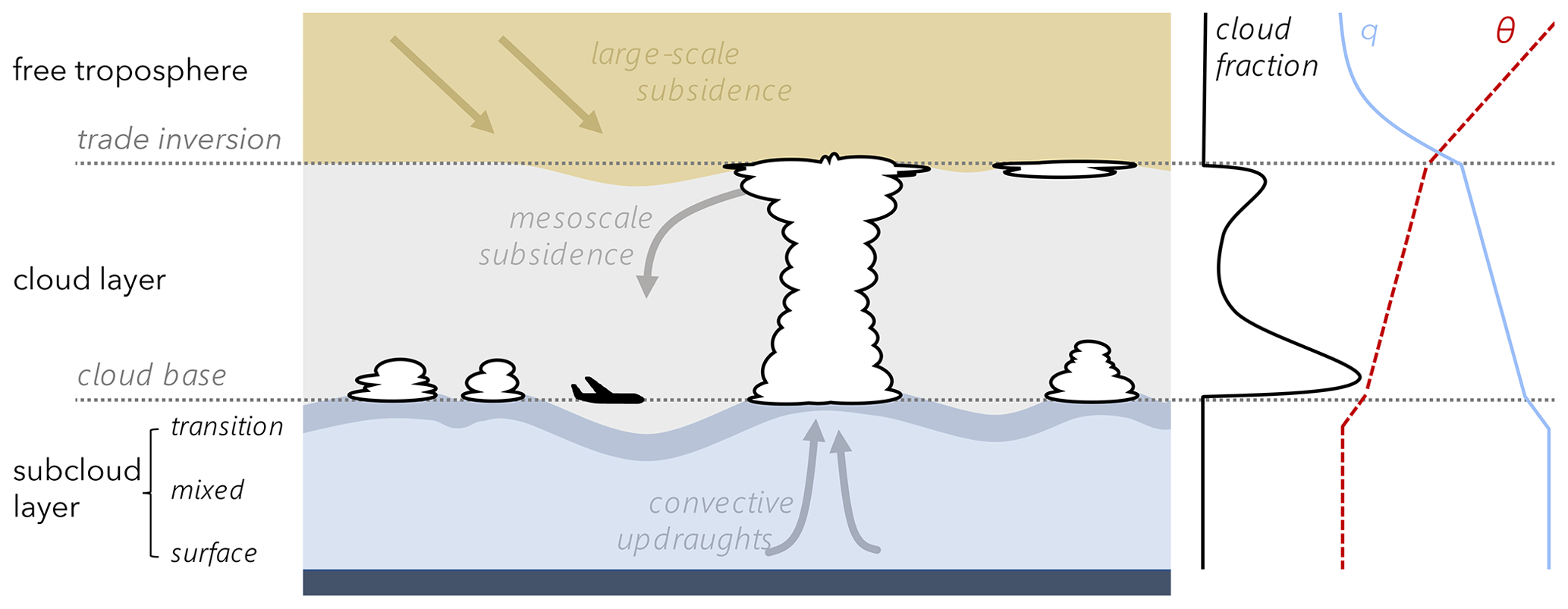
Figure 1 Schematic of the different atmospheric layers in the troposphere over the tropical Atlantic with the ATR aircraft flying at cloud base together with idealised profiles of cloud fraction (black), specific humidity (blue), and potential temperature (dashed red). Based on the ATR measurement time series shown in Fig. 12, we assume that the cloud base/subcloud layer top is characterised by an uneven topography instead of being a flat surface. See the text for the description of the individual layers.

Directly adjunct to the subcloud layer top is the cloud base level, where clouds start to form and may grow vertically until reaching the trade inversion, which represents the upper bound of the cloud layer. The horizontal extent of the clouds is typically largest at the cloud base, but, if the clouds develop up to the trade inversion level, a secondary maximum may emerge at their top in the form of stratiform outflows. This leads to a bimodal vertical distribution of cloud fraction (e.g. Vial et al., 2019). The contrasting radiative properties of the cloudy and clear-sky environments in the cloud layer can induce shallow circulations (Naumann et al., 2017), which in turn influence the properties of the subcloud layer below. Another process through which the cloud layer feeds back to the subcloud layer is the formation of evaporatively driven cold pools, which create cold-dry density currents that spread radially at the surface. They may initiate new convection at their edges through mechanical lifting and buoyancy caused by increased moisture contents (e.g. Tompkins, 2001; Schlemmer and Hohenegger, 2014; Torri et al., 2015; Vogel et al., 2021).

The trade inversion that caps the cloud layer forms due to the large-scale subsidence typically found in the free troposphere of the trade-wind region. This large-scale subsidence corresponds to the descending branch of the Hadley cell. The subsidence rate is determined by the balance between adiabatic warming and radiative cooling and is roughly 35 hPa d⁻¹ (Salathé and Hartmann, 1997; Holton and Hakim, 2013). Occasionally, however, the Hadley-cell-like descent is replaced by air masses descending much faster (∼ 200 hPa d⁻¹) from the extratropics along the slanted isentropes (Aemisegger et al., 2021b; Villiger et al., 2022).

Each of the above-described layers (Fig. 1) is characterised by a distinct isotopic composition of vapour. Generally, the vapour is more enriched in heavy isotopes closer to the surface. With increasing altitude, as soon as condensation and rainout occur, the vapour continuously loses its heavy isotopes and becomes lighter. The d-excess is assumed to be high near the ocean surface and to decrease with altitude due to a slight temperature dependency (Thurnherr et al., 2021). Once very dry conditions are reached (at about 12 km and above; this altitude was identified in vertical cross-sections (not shown) of the data from the numerical simulations described in Sect. 2), the non-linearity of the δ scale causes a rapid increase of the d-excess relative to the values observed near the surface (Dütsch et al., 2017). The large-scale circulation can substantially alter the isotopic composition (Aemisegger et al., 2021b) by influencing the conditions under which the vapour is evaporated from the ocean surface or by advecting air masses from other regions (e.g. more depleted air from higher latitudes).

At cloud base, different processes are at play, shaping the isotope variability. On the one hand, transport within mesoscale systems accumulates freshly evaporated and enriched vapour in areas where clouds are being formed and brings dry and depleted air from high altitudes to cloud base into the clear-sky environments between clouds (radiatively driven subsidence). The d-excess is expected to be high in convective updraughts bearing the signal of ocean evaporation and comparably lower for moisture in clear-sky environments, which has previously gone through cloud formation processes (i.e. moisture detrained from clouds). Note that in the shallow trade-wind cumuli regime, the air does not become dry enough for the non-linearity of the δ scale to affect the d-excess. On the other hand, microphysical processes, such as the formation of cloud droplets or the partial or full evaporation of cloud and rain droplets, impact the cloud vapour's isotope signal. If the formed condensate is removed from the cloud through precipitation, the cloud layer's total water gets depleted in heavy isotopes. The vapour in clear-sky environments is indirectly influenced by this process, as, ultimately, the cloudy air gets detrained into clear-sky environments and subsides back to cloud base. Both processes, mesoscale transport and microphysics, taken together, thus lead to contrasting isotope signals in cloudy and clear-sky environments at cloud base.

1.3 Earlier model evaluation studies

Several studies have evaluated the performance of models in the lower troposphere of the trade-wind region during EUREC⁴A. Beucher et al. (2022) tested the oversea configuration of the French regional model AROME, called AROME-OM (its output used by Dauhut et al., 2023, as initial and lateral boundary conditions for large-eddy simulations). In their model set-up, deep convection is treated explicitly, but shallow convection is parameterised. Beucher et al. (2022) found that AROME-OM produces a too deep subcloud layer associated with a dry bias (−1 g kg⁻¹ in specific humidity) and has a cold bias in the cloud layer (−0.5 K in potential temperature). Further, AROME-OM is able to produce stratiform clouds near the trade inversion, but their occurrence is underestimated. Besides identifying these shortcomings, Beucher et al. (2022) demonstrated the capacity of AROME-OM to predict the different mesoscale cloud organisation patterns and their associated environment. Savazzi et al. (2022) looked into lower-tropospheric biases of meridional winds in Integrated Forecasting System (IFS) forecasts and ERA5 reanalyses. They found a weak wind speed bias at altitudes below 5 km during local daytime and a strong wind speed bias below 2 km during local nighttime. Here, a further model evaluation in the framework of EUREC⁴A is added, with a focus on isotopes.

Since we are using COSMO_iso simulations, we summarise the most relevant findings from earlier model evaluation studies of COSMO and COSMO_iso used at the kilometre-scale resolution, albeit conducted mostly in regions other than the trades. Ban et al. (2014) showed that turning off the deep convection scheme leads to a more accurate diel cycle of surface temperature and precipitation over Europe. Vergara-Temprado et al. (2020) performed COSMO simulations over Europe at seven different horizontal grid spacings, ranging from 50 to 2.2 km. At each resolution, Vergara-Temprado et al. (2020) carried out one simulation with the full Tiedtke (1989) scheme, one with a parameterisation of shallow convection only, and another one without any convection parameterisation. They found that at grid spacings of 25 km or smaller, explicit convection improves the model skill with regard to surface temperature, precipitation, and top-of-atmosphere radiation. The improvement over the simulations with fully parameterised convection applies to both simulations with partly resolved (deep convection) and fully resolved convection (deep and shallow). Furthermore, the study showed that the representation of some variables strongly depends on the spatial resolution of the model, while for others the convection parameterisation settings (i.e. resolved vs. parameterised) are crucial. For example, hourly precipitation and outgoing long-wave radiation are mostly determined by whether the convection is resolved or parameterised, while net short-wave radiation is more sensitive to the spatial resolution (due to its strong dependence on cloud fraction). The grid-spacing sensitivity of COSMO was further investigated by Heim et al. (2021). They carried out five convection-resolving simulations over the tropical Atlantic with a grid spacing ranging from 12 km to 500 m and found, for instance, that the low-cloud fraction decreases with finer resolution.

The isotope-enabled version of COSMO has been used and evaluated previously in different regions but never in the tropical trade-wind region. Thurnherr et al. (2021) used COSMO_iso simulations with explicit convection over the Southern Ocean and compared them to ship-based and radiosonde measurements. They observed that the vapour in the lowest model level was too depleted and had too high d-excess values compared to in situ measurements (their Fig. 9). They argued that too strong vertical mixing possibly caused the observed bias and that the offset in d-excess could be reduced by using the smooth regime of the formulation by Merlivat and Jouzel (1979) for non-equilibrium fractionation instead of the formulation by Pfahl and Wernli (2009) developed with observations from the Mediterranean. Previous studies (e.g. Steen-Larsen et al., 2015; Aemisegger and Sjolte, 2018; Bonne et al., 2019) showed that using the non-equilibrium fractionation factor corresponding to the smooth regime in the Merlivat and Jouzel (1979) formulation provides the most reliable results.

Dahinden et al. (2021) and de Vries et al. (2022) evaluated the humidity and isotope signals of COSMO_iso in the free troposphere in the context of the west African monsoon. Dahinden et al. (2021), who used a set-up with resolved convection in the vicinity of the Canary Islands, found that COSMO_iso is overly moist and enriched at altitudes ≥6 km compared to in situ aircraft observations. However, the day-to-day variability of the humidity and δ²H of COSMO_iso agreed well with ground-based remote sensing observations from Tenerife (FTIR). de Vries et al. (2022) performed three COSMO_iso simulations in the west African monsoon region and tested the effect of parameterised versus explicit convection and different spatial resolutions. Independent of the modelling set-up, COSMO_iso produced a distinct bias towards too high δ²H at 4.2 km compared to satellite-based remote sensing observations from IASI (Infrared Atmospheric Sounding Interferometer; Schneider and Hase, 2011). Despite the offset, the temporal evolution of the simulations agreed well with the observations, lending confidence to the model's ability to reproduce the mesoscale to synoptic-scale variability in the water vapour isotope fields.

The literature summarised above suggests that simulations should be done by using an explicit representation of convection, and a fine spatial resolution should be used for variables such as the cloud fraction (Ban et al., 2014; Vergara-Temprado et al., 2020; Heim et al., 2021), albeit without expecting a significant improvement for water vapour isotope variables (de Vries et al., 2022). Furthermore, we anticipate a depletion bias in the near-surface vapour (Thurnherr et al., 2021) and an enriched bias in the free-tropospheric vapour but overall a good performance in terms of the mesoscale to synoptic-scale variability in humidity and isotope variables (Dahinden et al., 2021; de Vries et al., 2022). Motivated by the consideration by Thurnherr et al. (2021), we used the smooth regime of Merlivat and Jouzel (1979) in our simulations to formulate non-equilibrium fractionation during evaporation from the ocean surface. Furthermore, we applied a nested model set-up, because earlier isotope-enabled modelling studies in the tropics that used a radiative–convective equilibrium set-up (Bony et al., 2008; Risi et al., 2008; Blossey et al., 2010) produced a negative bias in heavy isotopes of precipitation (Bony et al., 2008; Torri et al., 2017).

2 Data and methods

2.1 Numerical simulations

We carried out three simulations with explicit convection and with different grid resolutions (10, 5, and 1 km) using the regional model COSMO_iso. The implementation of isotopes in COSMO_iso is achieved through a parallel water cycle for each of the two heavy isotopes (Pfahl et al., 2012), ¹H²H¹⁶O and ¹H${}_{\mathrm{2}}^{\mathrm{18}}$O, which differs from the one of ¹H${}_{\mathrm{2}}^{\mathrm{16}}$O by accounting for fractionation processes. The two additional water cycles are purely diagnostic and do not affect other model components. Fractionation processes during soil water evaporation are included through the coupling of COSMO_iso and TERRA_iso, an isotope-enabled prognostic multilayer soil model (for details, see Christner et al., 2018). Plant transpiration is treated as a non-fractionating process (Aemisegger et al., 2015). For evaporation from the ocean surface, the non-equilibrium fractionation factors from the smooth regime of Merlivat and Jouzel (1979) were used. Cloud processes were simulated by a one-moment microphysics scheme with a fixed number of cloud droplets ($N_{\mathrm{c}}=\mathrm{5}\times {\mathrm{10}}^{\mathrm{8}}$ m⁻³; Doms et al., 2011). The convection schemes of the model (Tiedtke, 1989; Theunert and Seifert, 2006) were disabled, meaning that deep and shallow convection were treated explicitly at the grid scale. A 20 s model time step was used, and hourly output was generated. A nested approach with spectral nudging of horizontal winds in the free troposphere was chosen to allow for a direct comparison to observations and to correctly capture influences from large-scale advection via the lateral boundary conditions.

The initial and lateral boundary conditions for the COSMO_iso simulation with the coarsest spatial resolution, referred to as COSMO_iso,10 km, were taken at 6-hourly intervals from a simulation performed with the global model ECHAM6-wiso (Cauquoin et al., 2019; Cauquoin and Werner, 2021). To reproduce the large-scale meteorological conditions during EUREC⁴A, ECHAM6-wiso was nudged (including surface pressure, temperature, and horizontal winds) towards ERA5 (Hersbach et al., 2020). The ECHAM6-wiso simulation was performed with parameterised convection and used the wind-dependent non-equilibrium fractionation factors from Merlivat and Jouzel (1979) for evaporation from the ocean surface. The global model was run with the spectral grid T127 (approx. 0.9^∘ horizontal resolution) and 95 vertical levels.

COSMO_iso,10 km has a horizontal resolution of 0.1^∘, has 40 vertical levels, and covers most of the North Atlantic (Fig. 2, Table 1). Horizontal winds above 850 hPa in COSMO_iso,10 km were nudged towards ECHAM6-wiso. The spectral nudging technique ensured that the regional simulations remain close to the large-scale flow in the global model (Von Storch et al., 2000; Schubert-Frisius et al., 2017). The nudging included only zonal and meridional wave numbers of less than five. COSMO_iso,10 km covers the period from 6 January to 13 February 2020. The first 10 d are treated as spin-up and are not included in the analysis.

Table 1 Model set-up for the ECHAM6-wiso, COSMO_iso,10 km, COSMO_iso,5 km, and COSMO_iso,1 km simulations. The following abbreviations are used to describe the variables included in the nudging: surface pressure (SP), temperature (T), zonal wind component (U), and meridional wind component (V).

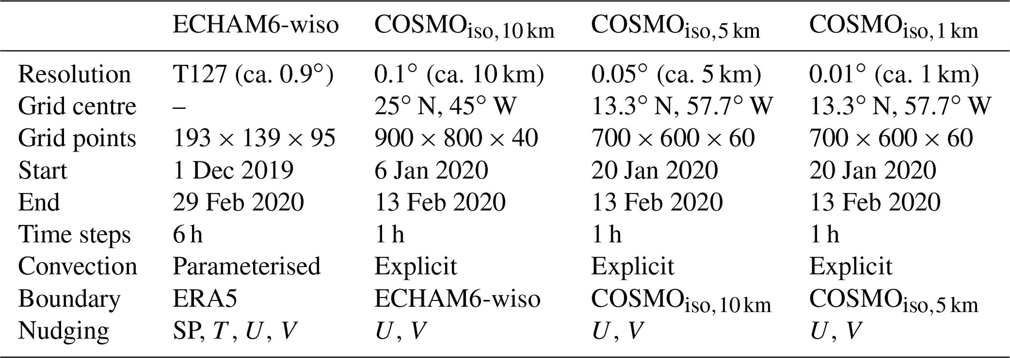
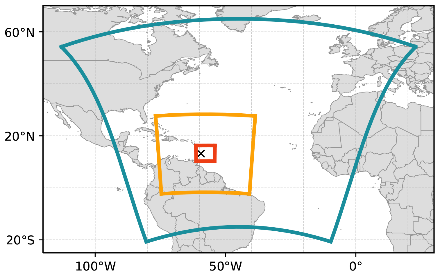
Figure 2 Domain boundaries of the three COSMO_iso simulations, i.e. COSMO_iso,10 km (teal), COSMO_iso,5 km (orange), and COSMO_iso,1 km (red). The location of Barbados is indicated by a black cross.

The second COSMO_iso simulation, COSMO_iso,5 km, has a horizontal resolution of 0.05^∘, has 60 vertical levels, and covers a subset of the western North Atlantic, including the northern part of the South American continent (Fig. 2, Table 1). Initial and lateral boundary conditions were taken from COSMO_iso,10 km at hourly time steps. The spectral nudging technique was identical to the first COSMO_iso simulation but nudged towards COSMO_iso,10 km horizontal winds above 850 hPa instead of ECHAM6-wiso (using the same wave numbers as for COSMO_iso,10 km, albeit resulting in smaller wavelengths given the smaller model domain). COSMO_iso,5 km covers the period from 20 January to 13 February 2020. All simulated days are included in the analysis.

The third COSMO_iso simulation, COSMO_iso,1 km, has a horizontal resolution of 0.01^∘, has 60 vertical levels, and covers the focus area of the field activity of EUREC⁴A (Fig. 2, Table 1). Initial and lateral boundary conditions were taken from COSMO_iso,5 km at hourly time steps. The spectral nudging, in this case, was directed towards COSMO_iso,5 km wind data. COSMO_iso,1 km covers the period from 20 January to 13 February 2020, and all simulated days are taken into account for the analysis.

2.2 Observational datasets

2.2.1 Satellite observations

The true-colour images from the Visible Infrared Imaging Radiometer Suite (VIIRS) on board the polar-orbiting satellite Suomi-NPP (National Polar-orbiting Partnership; NOAA, 2017) are used to assess the spatial organisation of clouds. The images were retrieved from the Worldview Snapshot application on NASA's Earthdata platform. For the same purpose, the data (with a spatial resolution of 500 m) from the visible channel of the satellite GOES-16, which is part of NOAA and NASA’s Geostationary Operational Environmental Satellite (GOES) – R Series, were downloaded from the EUREC⁴A data catalogue.

The Integrated Multi-satellitE Retrievals (IMERG) from the Global Precipitation Measurement (GPM) mission is used for the evaluation of the spatial distribution of precipitation. We refer to the data, which were obtained from NASA’s Earthdata platform, simply as GPM. Here, the half-hourly (Huffman et al., 2019a) and daily (Huffman et al., 2019b) precipitation estimates are used.

2.2.2 Aircraft observations

Several observational datasets that were created during EUREC⁴A on board the ATR and the German aircraft HALO (High Altitude and Long Range Research Aircraft; Konow et al., 2021) are used. All of them are available on AERIS (https://eurec4a.aeris-data.fr, last access: 18 September 2022). The ATR conducted 19 flights on 11 d from 25 January to 13 February 2020. A flight typically lasted 4 to 5 h and consisted of repetitive flight patterns. They included the ferry from the Grantley Adams International Airport of Barbados into the western half of the so-called EUREC⁴A circle (see definition below), followed by two or three rectangles (120 km × 20 km) at cloud base, one or two L-patterns flown either near the top or the middle of the subcloud layer, occasionally a surface leg at an altitude of about 60 m, and the ferry back to the airport, which often included a short leg above the trade inversion to sample free tropospheric air. The ATR flights were closely coordinated with those of HALO, which performed 15 flights from 19 January to 18 February 2020. Each HALO flight lasted about 9 h, seven of which the aircraft spent at upper altitudes (∼ 10 km) in the EUREC⁴A circle centred at 13.3^∘ N, 57.7^∘ W (roughly 150 km east of Barbados), with a diameter of ∼ 220 km. When HALO was flying this circle, dropsondes were launched frequently to estimate the large-scale vertical motions (Bony and Stevens, 2019; Stevens et al., 2021; Konow et al., 2021; George et al., 2021a, 2023). HALO dropsonde data (George et al., 2021b) are used for the evaluation of the COSMO_iso simulations.

The ATR's position and the corresponding standard meteorological variables (e.g. pressure, temperature, wind components) are reported in the CORE dataset (CNRM/TRAMM et al., 2021; Bony et al., 2022,  at 1 Hz temporal resolution). Considering that the ATR moved roughly 100 m s⁻¹, the spatial resolution of its observations amounts to 100 m for the 1 Hz data and to 1 km for the 10 s averaged data.

The ATR-based BASTALIAS dataset (Delanoë et al., 2021) is used for the evaluation of the cloud fraction at cloud base. It is a data product resulting from the combined observations of the Doppler cloud radar BASTA (Bistatic Radar System for Atmospheric Studies; Delanoë et al., 2016) and the lightweight backscatter lidar ALiAS (Airborne Lidar for Atmospheric Studies; Chazette et al., 2020) that were horizontally probing the surroundings of the ATR.

The ATR-based PMA dataset (Microphysics Airborne Platform; Coutris, 2021,  at 1 Hz temporal resolution) is used for the microphysical characterisation of the clouds and their surroundings. It contains the combined observations from an optical-scattering droplet spectrometer (Lance et al., 2010) and an optical array stereo probe imager (Lawson et al., 2006), together sizing and counting the droplets with diameters from 2 µm to 2 mm. From the size distribution composites of the two instruments, the total concentration of particles; the median volume diameter; the liquid water content (LWC); and flags indicating the presence of cloud, drizzle, or raindrops are inferred. Cloud drops are identified if the LWC exceeds 10 mg m⁻³ and the particle diameter remains below 100 µm; drizzle is identified if the LWC exceeds 10 mg m⁻³ and the particle diameter is at least 100 µm but remains below 500 µm; and rain is identified if the LWC exceeds 10 mg m⁻³ and the particle diameter exceeds 500 µm.

Finally, the ATR-based Picarro dataset (Aemisegger et al., 2021a) is used for the humidity conditions and the isotopic composition of the vapour, which were both measured with a customised cavity ring-down spectrometer, L2130-i, from the manufacturer Picarro with a sampling frequency of 1 Hz (more technical details in Bailey et al., 2023). The Picarro dataset provides a flag indicating data points of questionable quality (e.g. due to inlet wetting). These data points were removed for the analyses shown in this paper. Moreover, only 10 s averages (for a better noise-to-signal ratio) are used, which corresponds to an effective horizontal resolution of 1 km and thus makes the observations comparable to the COSMO_iso,1 km simulation.

Note that the ATR observations have been thoroughly evaluated in Bony et al. (2022). They found that the different ATR measurements of humidity, wind, and cloud fraction are in good agreement with each other and with HALO dropsondes.

2.3 Definition of the cloud base level

The ATR data come with an official flight segmentation (Bony et al., 2022). Here, we use the data that are labelled as cloud base. The targeted cloud base level was determined before each flight based on ceilometer, radio sounding, and surface weather observations as well as satellite imagery. During the flight, the altitude was fine-tuned based on real-time measurements and visual impressions. To ensure that only the data points collected at the base of shallow clouds are taken into account, we apply the criterion that only data points with altitudes below 1.3 km (threshold for the distinction between shallow and deep clouds used in Vial et al., 2019) are treated as cloud base observations. The resulting cloud base mean and median pressure for each flight are shown in Fig. 3.

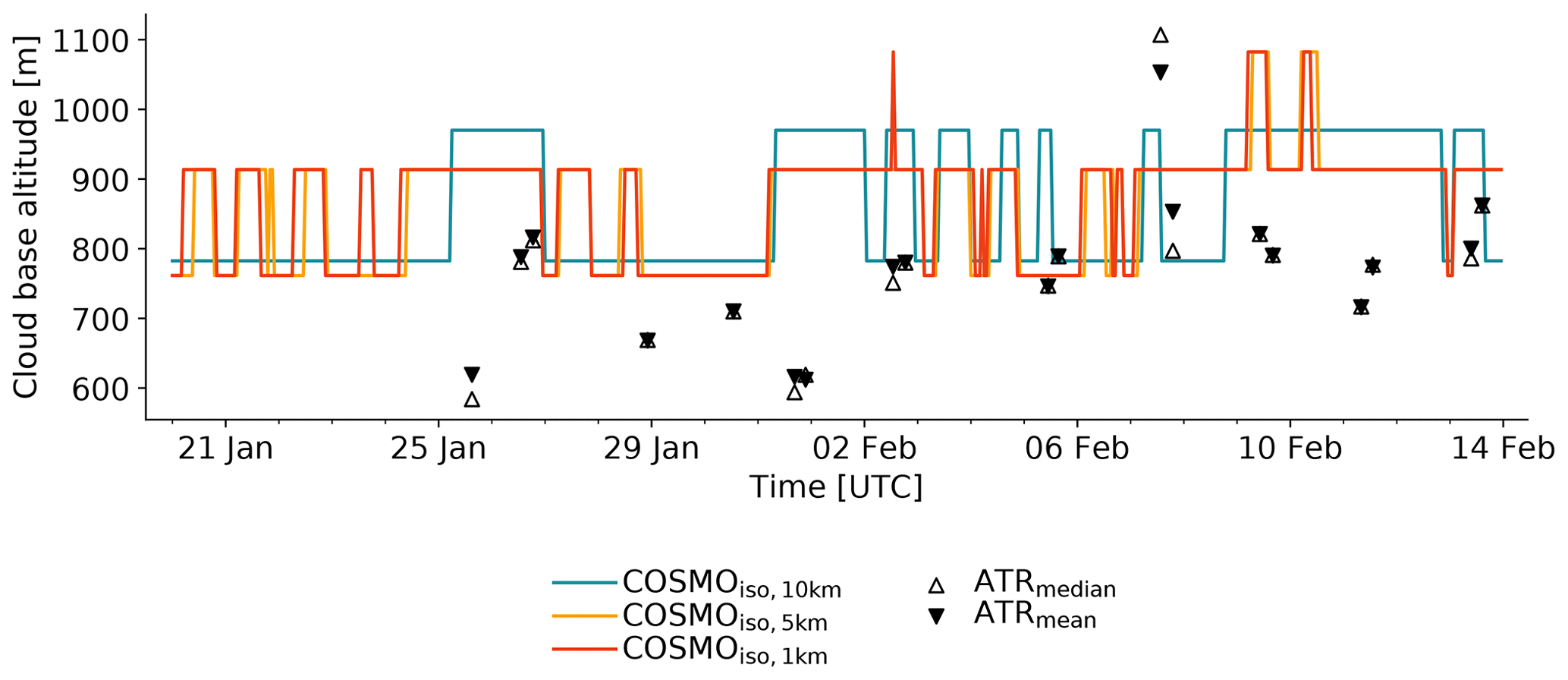
Figure 3 Time series of cloud base COSMO_iso model level and ATR flight altitude. Shown are the median values of the grid points in the domain 54.5–61^∘ W and 11–16^∘ N at every hourly time step for COSMO_iso,10 km (teal), COSMO_iso,5 km (orange), and COSMO_iso,1 km (red), as well as the median (empty black markers) and mean (filled black markers) value of each ATR flight.

For comparison with the ATR data, a model level representing cloud base in the domain 54.5–61^∘ W and 11–16^∘ N is defined for the COSMO_iso simulations. This model level is identified for every hourly time step individually, following the steps below:

1. Every vertical profile in the domain 54.5–61^∘ W and 11–16^∘ N is checked for cloud water content exceeding 10 mg kg⁻¹ (threshold for the detection of clouds used in Vial et al., 2019) at any model level below 1.3 km. The lowest model level meeting this criterion is taken as the cloud base of the respective vertical profile. If the profile does not contain any clouds, it is ignored in the subsequent step.

2. In order to extract cloud base conditions, we determine one cloud base model level for the domain 54.5–61^∘ W and 11–16^∘ N by calculating the median over the cloud base model levels identified for cloudy profiles in the previous step.

3. Steps 1 and 2 are repeated for every hourly time step of the simulated time period. The resulting time series of cloud base model levels can then be used to extract cloud base variables (as, for example, pressure shown in Fig. 3) from the COSMO_iso simulations.

The cloud base levels identified in the three COSMO_iso simulations, using the procedure described above, alternate between the model levels 29 (783 m) and 30 (970 m) for COSMO_iso,10 km and 47 (761 m), 48 (914 m), and 49 (1082 m) for COSMO_iso,5 km and COSMO_iso,1 km. COSMO_iso underestimates the flight-to-flight variability of the cloud base altitude in comparison to the ATR data (Fig. 3). Nevertheless, the identified COSMO_iso cloud base altitudes are in the range of the values observed by the ATR during the cloud base flight segments (Fig. 3b). Therefore, the COSMO_iso cloud base data are assumed to be comparable to the ATR cloud base data.

3 Model evaluation and spatial resolution effects

EUREC⁴A offers a unique opportunity to perform a thorough evaluation of model simulations targeted at shallow trade-wind cumulus clouds in a process-oriented way thanks to the wealth of available observational data. In the following, variables from the different COSMO_iso simulations, which are considered to be relevant for the formation of shallow cumulus clouds in the trade-wind region, are selected and compared to observations. Simultaneously, the effect of the spatial model resolution is assessed, without upscaling outputs from the higher resolution simulations to the lowest resolution. All comparisons are performed with the data in the selected evaluation domain 54.5–61^∘ W and 11–16^∘ N (corresponding approximatively the domain of the COSMO_iso,1 km simulation). This domain was chosen large enough to provide a robust statistical basis to analyse cloud properties while remaining small enough to contain a fairly homogeneous cloud field in terms of cloud patterns.

3.1 Clouds and precipitation

The COSMO_iso simulations are all able to distinguish between different mesoscale organisation patterns (Fig. 4; other dates can be found in Fig. S1.2–S1.11 in Supplement 1). Note that the model is not expected to produce clouds identical to the ones in the observations, but it is plausible that the simulations reproduce the mesoscale cloud organisation patterns since they are linked to distinct large-scale environmental conditions (Bony et al., 2020). The elongated Fish clouds on 22 and 26 January 2020 are reproduced by COSMO_iso, although at a different location than depicted by the satellite image, hinting towards slight errors in the propagation speed of the banded clouds associated with trailing cold fronts (see Villiger et al., 2022, for the link between Fish clouds and trailing cold fronts). On 12 February 2020, the satellite shows large Flower clouds, which are not clearly identifiable in the COSMO_iso output. Nevertheless, if viewed over a larger domain (Supplement 1), aggregated cloud liquid water content objects are visible, resembling Flower clouds. Smaller Flower clouds, as on 2 February 2020, are clearly reproduced by the model. Finally, more finely structured cloud patterns recognised as Gravel and Sugar, as they appear on 8 and 9 February 2020 in the satellite observations, are also reproduced by COSMO_iso. Note that the cloud classification used above largely agrees with the patterns identified by Schulz (2022, their Fig. 7a).

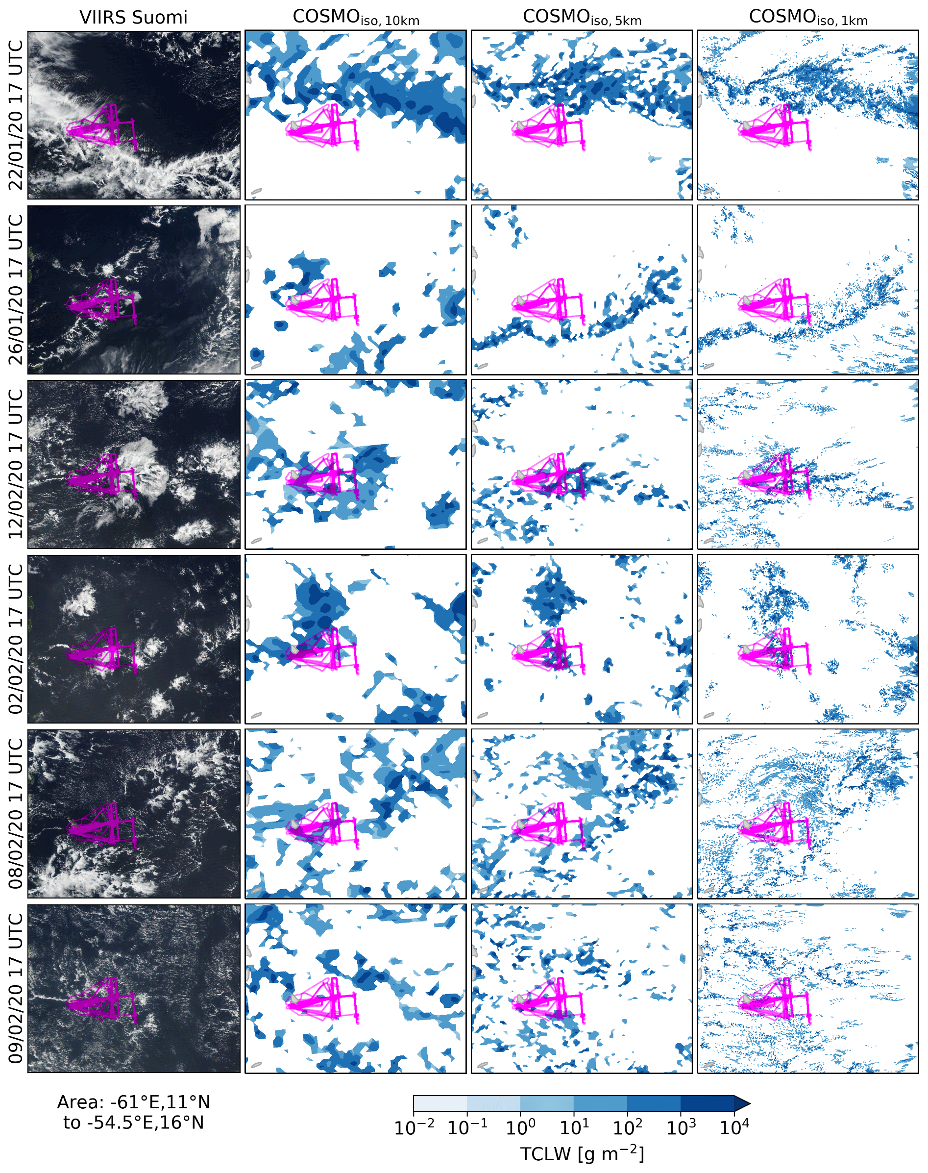
Figure 4 Spatial organisation of the clouds in the domain 54.5–61^∘ W and 11–16^∘ N from four datasets (columns) and on six dates (rows). The first column shows the image from the VIIRS instrument on board the polar-orbiting Suomi-NPP satellite (approx. equatorial crossing time 17:30 UTC). The remaining columns show the total column cloud liquid water (TCLW) in the three COSMO_iso simulations at 17:00 UTC. The dates are chosen according to the displayed cloud species, with large/small Fish clouds on 22/26 January 2020, large/small Flower clouds on 12/2 February 2020, and Gravel-Sugar/Sugar clouds on 8/9 February 2020. The track from all ATR flights is overlaid in pink. Other examples are shown in Supplement 1.

Overall, the spatial cloud patterns from the satellite images are qualitatively better reproduced by the simulations if the horizontal model resolution is increased. This holds true especially for the finely structured clouds on 8 and 9 February 2020. For these cases, only COSMO_iso,1 km shows the Gravel-typical cold-pool activity in the form of cloud liquid water arranged in arc-like structures around clear-sky patches. An exception is 12 February 2020, a day on which the organisation of the clouds in large Flowers is partially lost with the higher resolution of COSMO_iso,1 km.

The four mesoscale organisation patterns discussed above are known to be characterised by different low-level cloud fractions (Bony et al., 2020), peaking at different times of the day (Vial et al., 2021). Therefore, the temporal evolution of cloud fraction at cloud base is another measure to evaluate the performance of the three COSMO_iso simulations. In all three simulations, the variable is characterised by a pronounced diel cycle, with maximum cloud fraction during local early morning (Fig. 5; agreeing with Vial et al., 2019). The magnitude of the cloud fraction, however, is very different for the three simulations. The cloud fraction is largest in COSMO_iso,10 km and becomes progressively smaller with higher resolution until reaching minimum values in COSMO_iso,1 km. This behaviour is expected for clouds that are smaller than the grid resolution (explanatory sketch in Supplement 1) and has been observed in earlier studies (Hentgen, 2019; Heim et al., 2021). The motivation for displaying cloud fractions from all three simulations is to assess at which resolution we obtain cloud fractions that approximate the observations within their uncertainty range. The comparison to the ATR-based cloud fraction estimates (symbols in Fig. 5) shows that COSMO_iso,10 km and (for most of the flights) COSMO_iso,5 km overestimate cloud fraction. Contrastingly, COSMO_iso,1 km agrees well with ATR${}_{\mathrm{BASTALIAS},\mathrm{cloud}+\mathrm{drizzle}}$ except for the first flight on 2 February and the two flights on 7 February 2020. On these two dates, however, coarse cloud patterns (Flower and Fish; not shown) were present, meaning that the ATR likely underestimated cloud fraction due to its limited sampling area.

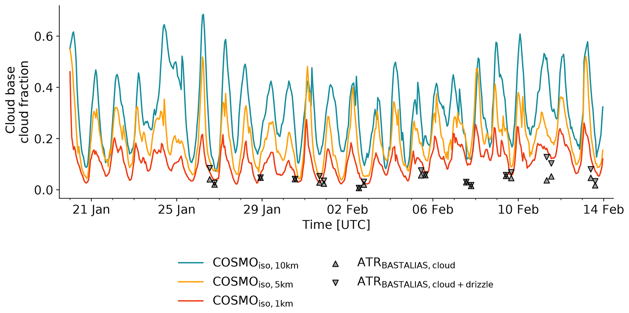
Figure 5 Time series of cloud fraction at cloud base for COSMO_iso,10 km (teal), COSMO_iso,5 km (orange), COSMO_iso,1 km (red), and the ATR (black markers). For COSMO_iso, the cloud fraction is calculated as the fraction of cloud base grid points in the domain 54.5–61^∘ W and 11–16^∘ N with cloud water content exceeding 10 mg kg⁻¹. The number of grid points in the considered domain are 3221 for COSMO_iso,10 km, 12 632 for COSMO_iso,5 km, and 316028 for COSMO_iso,1 km.

In the model, liquid water droplets in a grid cell are separated into the non-sedimenting cloud water content and the sedimenting rain water content, respectively. For comparison to the ATR-based liquid water content (LWC) measurements provided in the PMA dataset (Fig. 6a), the simulated cloud and rain water contents are summed up. Consistent with cloud base cloud fraction, the fractions of data points with the LWC > 10 mg kg⁻¹ are decreasing with increasing spatial model resolution and overall higher in the simulations than in the observations. COSMO_iso,10 km meets the threshold at 22.3 % of the data points, with COSMO_iso,5 km at 14.0 %, COSMO_iso,1 km at 8.3 %, and PMA at 5.6 %.

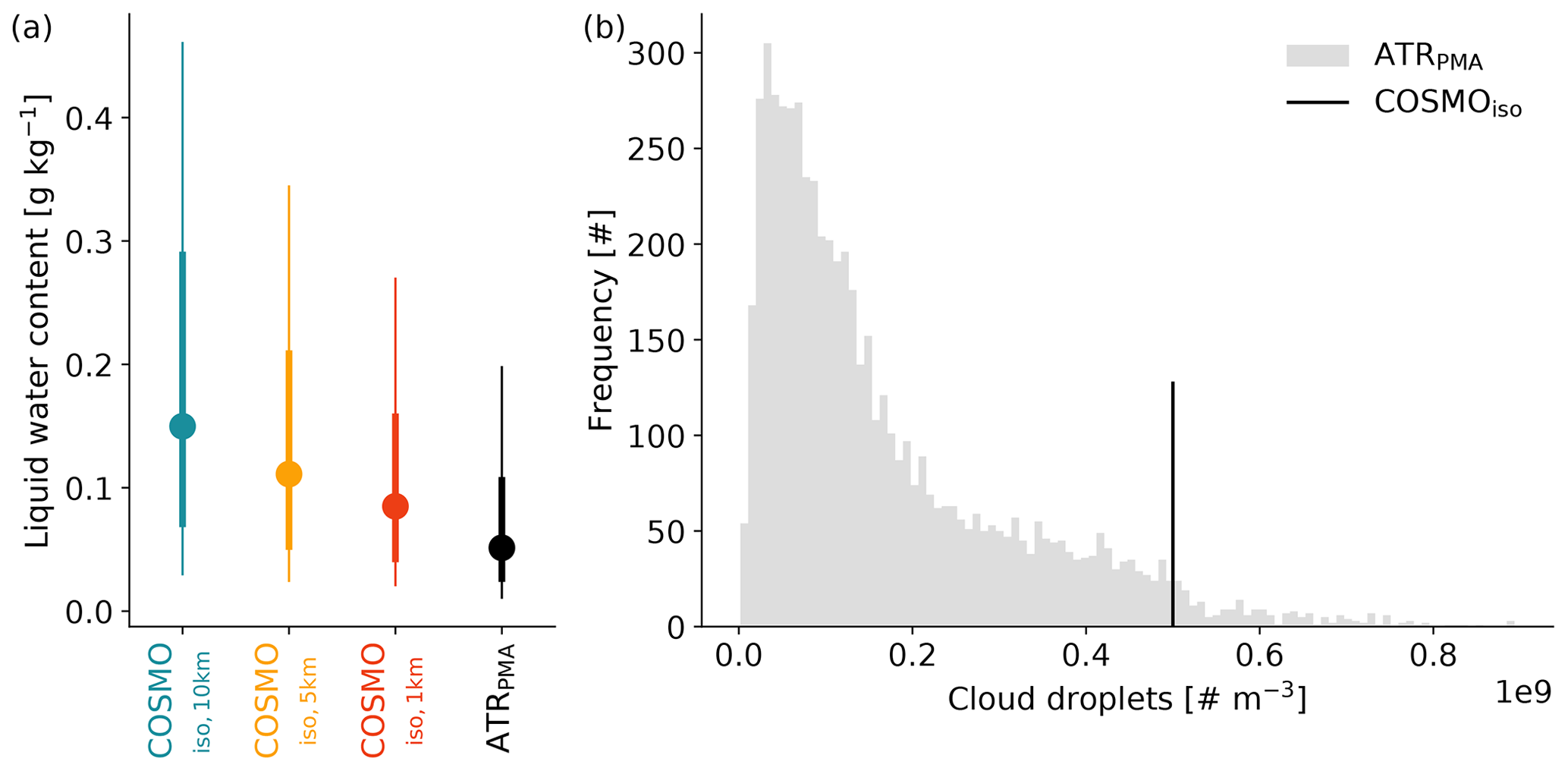
Figure 6 Distributions at cloud base of (a) liquid water content (LWC) from COSMO_iso,10 km (teal), COSMO_iso,5 km (orange), COSMO_iso,1 km (red), and ATR_PMA (black); and (b) cloud droplet numbers from COSMO_iso (black) and ATR_PMA (grey). For COSMO_iso, the LWC is calculated as the sum of cloud water content (CWC) and rainwater content (RWC; that is, LWC = CWC + RWC). Shown are (a) the 10th to 90th percentile range (thin vertical line), 25th to 75th percentile range (thick vertical line), and the median (marker) of all cloud base data points with LWC >10 mg kg⁻¹. For the ATR_PMA dataset, all flights (RF02–RF20) are taken into account; for COSMO_iso, the data in the domain 54.5–61^∘ W and 11–16^∘ N from the hourly time steps that are closest to the ATR flights are taken into account. In panel (b), the droplet number distribution from the ATR_PMA dataset during time steps flagged as cloud is shown together with the constant cloud droplet number of the one-moment cloud scheme of COSMO_iso.

The LWC at cloud base is generally overestimated in COSMO_iso compared to the observations, but the observed values are approached with increasing horizontal model resolution (Fig. 6a). Possibly, the number of cloud droplets (N_c), which is fixed to 5×10⁸ m⁻³ in the one-moment cloud scheme (Sect. 2), contributes to the offset between simulations and observations. This value is located at the upper end of the observed droplet number distribution (Fig. 6b). A high N_c leads to a reduction of the cloud droplets' size since the available liquid water is distributed over more droplets. This, in turn, reduces the efficiency of the collisional growth process and can delay or even prevent the formation of precipitation (see Eirund et al., 2022). In other words, N_c directly affects the autoconversion rate, the rate at which COSMO_iso turns cloud water into rain water. Thus, if the parameter were to be adjusted towards the observations, precipitation would likely be formed more readily (efficiently removing liquid water from the atmosphere), possibly affecting below-cloud evaporation of hydrometeors and surface precipitation. It remains to be tested how COSMO_iso would react to a change of N_c in the considered regime.

Figure 7 shows the rain water that ultimately reaches the surface. Compared to the satellite product, precipitation falls over smaller areas in COSMO_iso, even if the resolutions of the compared datasets are comparable (COSMO_iso,10 km vs. GPM; keep in mind that the satellite product is an estimate of surface precipitation and should not be taken as the absolute truth). The patches with intense rainfall become smaller and more frequent with finer model resolution. Most likely, this is due to an intensification of updraughts with finer model resolution.

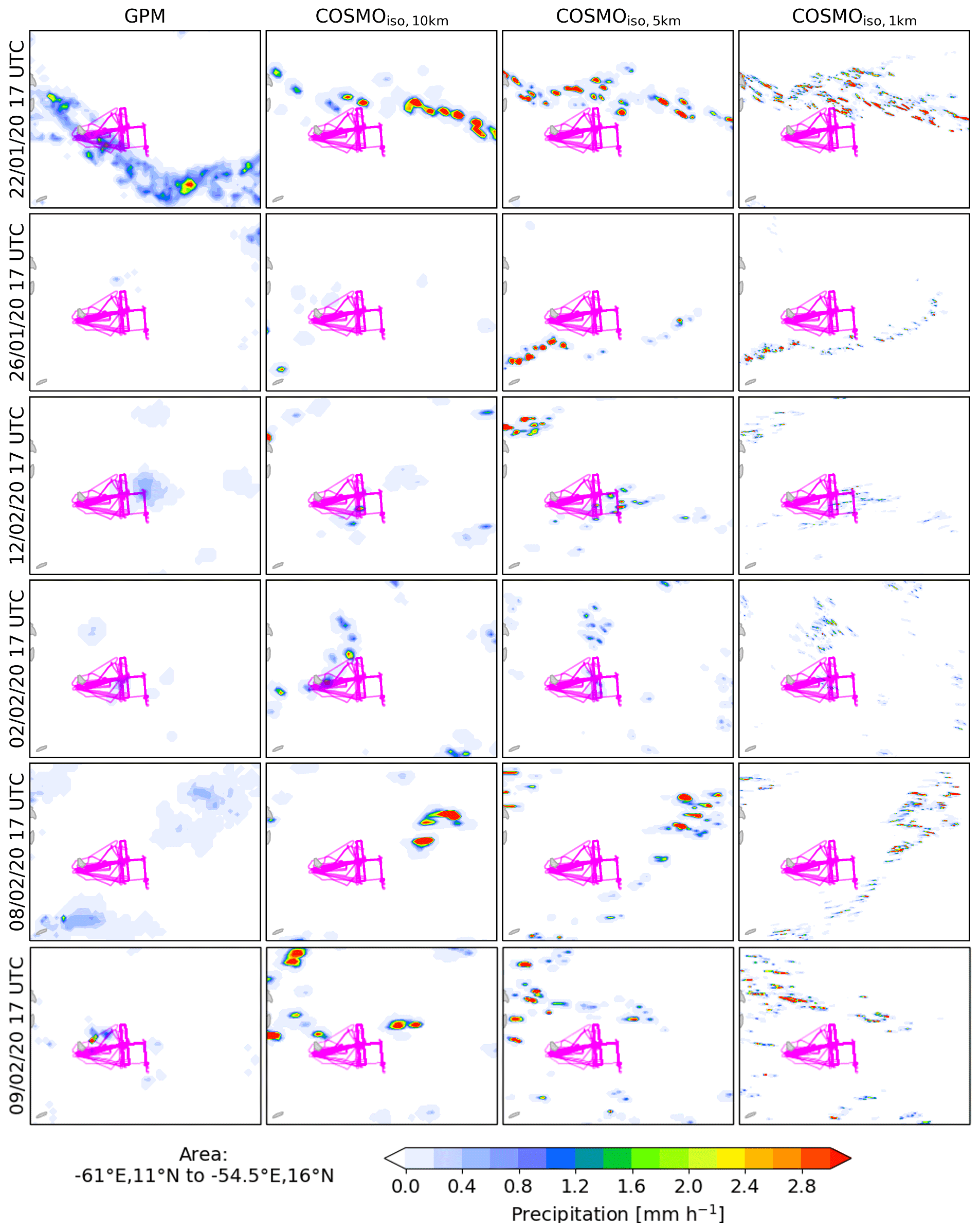
Figure 7 Hourly precipitation in the domain 54.5–61^∘ W and 11–16^∘ N from four datasets (columns) and on six dates (rows; also shown in Fig. 4). The first column shows the satellite-based precipitation estimate GPM (IMERG). The remaining columns show precipitation from the three COSMO_iso simulations from 16:00–17:00 UTC.

Considering that the spatial distribution of precipitation in COSMO_iso strongly contrasts with the satellite product (Fig. 7), the rainfall amounts over the evaluation domain are surprisingly close to each other (Fig. 8). It depends on the dominant cloud pattern, whether COSMO_iso is overestimating/underestimating precipitation, and whether the grid resolution has a systematic effect. From 20 to 24 January, when Fish clouds were dominant (Schulz, 2022, their Fig. 7), the simulations show a distinct diel cycle of precipitation (peaking shortly after the peak in cloud fraction; agreeing with Vial et al., 2016), while the satellite reports a period of continuous rainfall (Fig. 8a). Over a 24 h window (Fig. 8b), this leads to a rainfall underestimation on 22 and 24 January 2020 by all three simulations, while on 20, 21, and 23 January 2020 alternately one of the three simulations best matches with the satellite. The exaggerated diel cycle of precipitation in the simulations highlights potentially too strong radiatively driven mesoscale circulations that may slow down the propagation of the trailing cold front into the tropics (cf., shifted position of the Fish cloud in the simulations compared to the observations; Fig. 4). Note that this period was characterised by anomalous large-scale transport (Villiger et al., 2022) with the precipitation-triggering process being dominated by large-scale convergence instead of isolated cells of shallow convection.

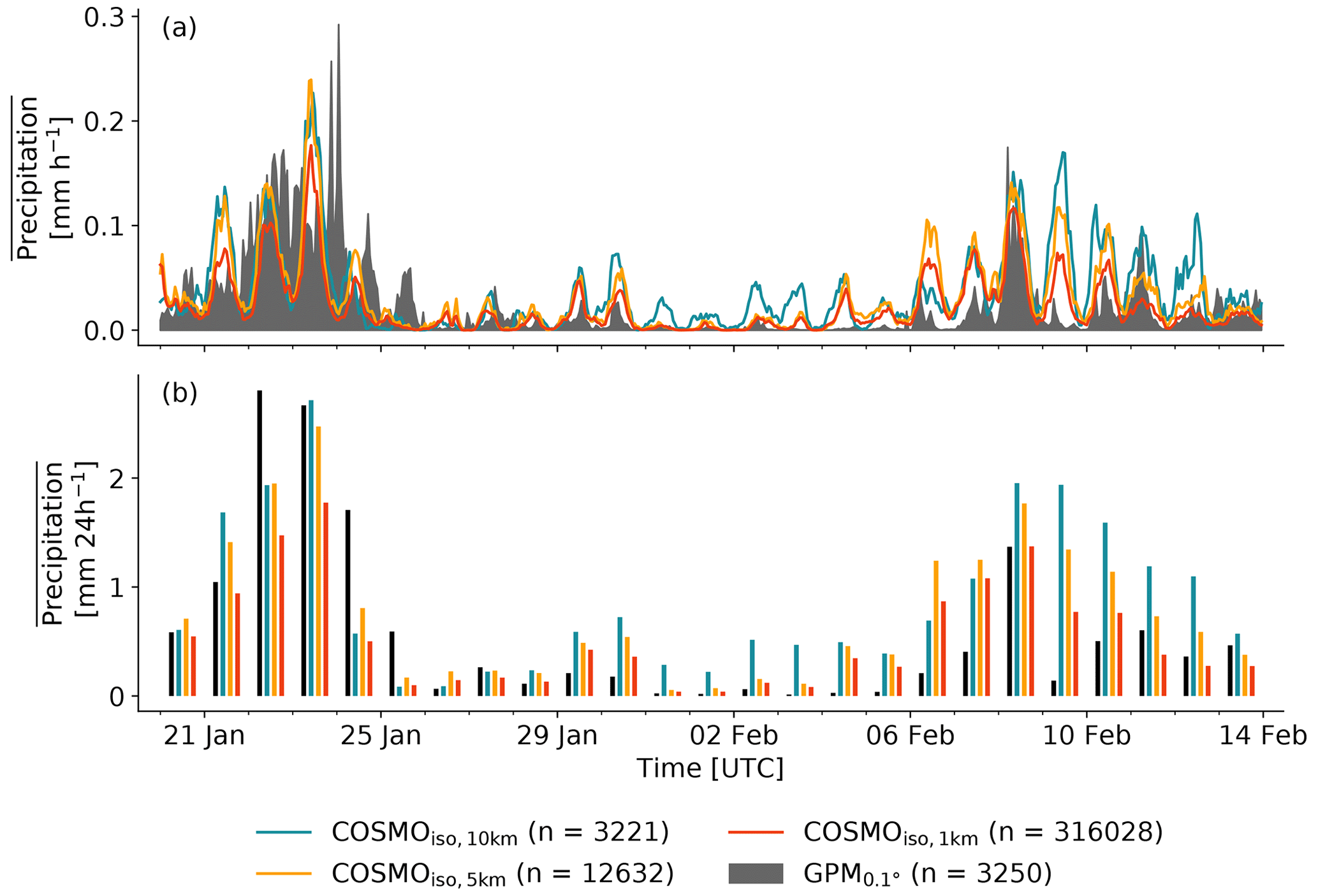
Figure 8 Time series displaying (a) hourly and (b) daily domain-averaged precipitation. Shown are the values from COSMO_iso,10 km (teal), COSMO_iso,5 km (orange), COSMO_iso,1 km (red), and GPM (black). Only the data in the domain 54.5–61^∘ W and 11–16^∘ N are taken into account. The number of grid points in the domain is given in round brackets.

From 25 January to 5 February 2020, when the clouds either are classified as Sugar or remain unclassified (Schulz, 2022, their Fig. 7), all COSMO_iso simulations overestimate the rainfall amount. The overestimation is smaller the finer the spatial model resolutions. From 6 February 2020 onwards, the rainfall amount is increased in all four datasets, but again none of the three simulations is exceptionally accurate. Much more, it depends on the date and which of the simulations is closest to the observations. This final period of the campaign was again characterised by anomalous large-scale transport (weak extratropical dry intrusion on 7 and 8 February 2020 and tropical mid-level detrainment starting on 12 February 2020, discussed in Villiger et al., 2022). The dominant cloud patterns in the considered domain were Fish clouds (7 to 8 February 2020) followed by Flower clouds (10 to 12 February 2020; Schulz, 2022, their Fig. 7). Besides 20 to 26 January 2020, the diel cycle of precipitation from COSMO_iso agrees with the one from the satellite observations (Fig. 8a).

The variables considered up to this point show a high dependence on the horizontal model resolution. This is not surprising since the three COSMO_iso simulations are in the so-called “grey zone” of resolutions, where only some of the scales involved in convective motions are resolved (Wyngaard, 2004), while the sub-grid-scale processes are taken care of by the turbulence scheme. This interplay between convection and turbulence leads to a strong resolution dependency of variables associated with convection (Hanley et al., 2015; Jeevanjee, 2017). Whether the increase in resolution leads to a better agreement with observations or not depends on the variable. For instance, the representation of the cloud parameters in the simulations is improved with finer resolution, while this is not the case for the spatial distribution of precipitation. For evaluations of large-eddy simulations with EUREC⁴A observations at even finer grid spacings than our COSMO_iso simulations, we refer to Schulz (2022).

3.2 Water vapour isotopes, humidity, and temperature

In contrast to the highly skewed variables discussed in the previous section, the close-to-normally distributed variables considered in this section are largely indifferent to model resolution (Figs. 9 and 10). This limited resolution dependence results from the fact that here we consider the full distribution of these variables and do not focus on the properties of subgrid-scale features as in the previous section.

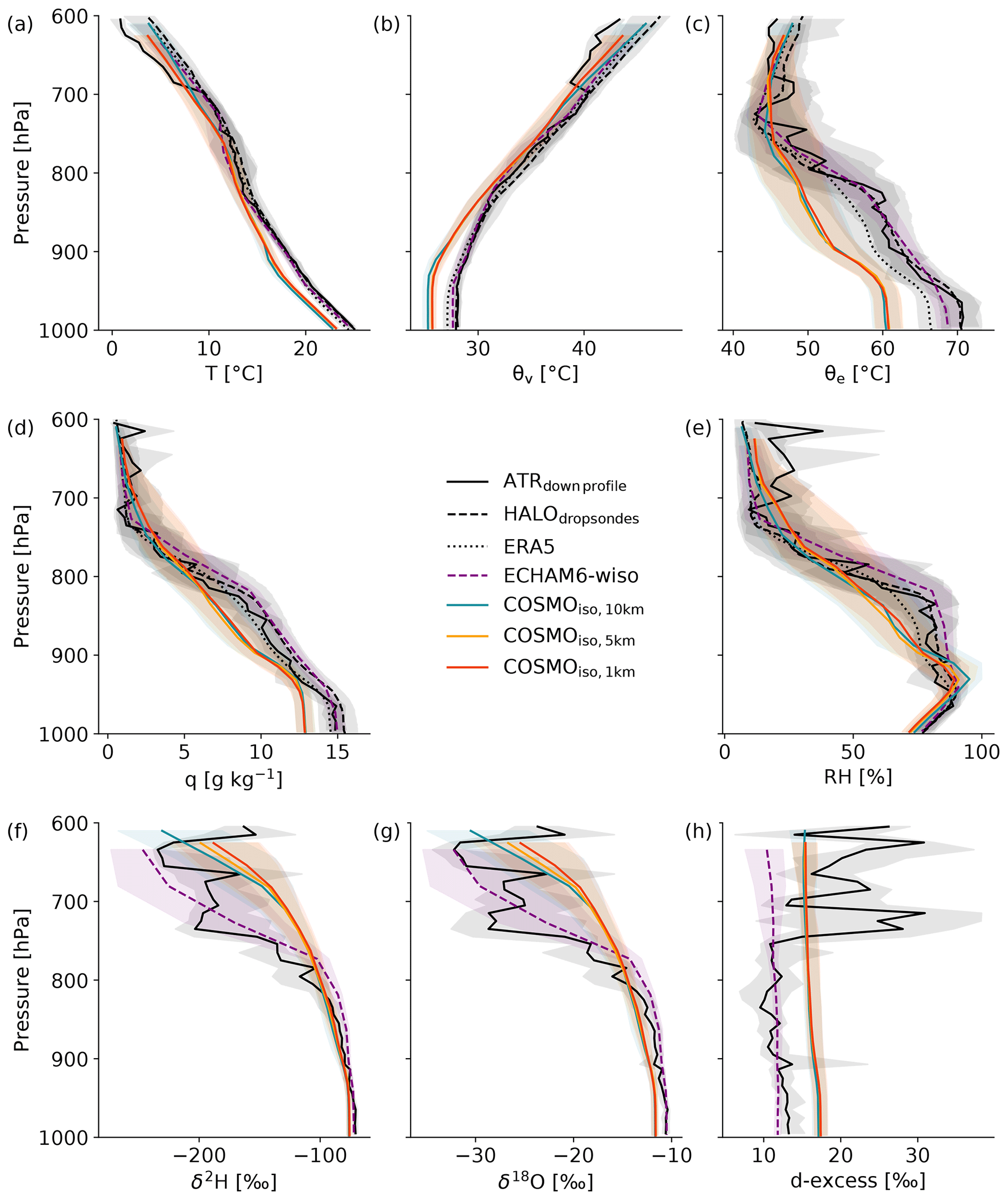
Figure 9 Vertical profiles of (a) temperature, (b) virtual potential temperature, (c) equivalent potential temperature, (d) specific humidity, (e) relative humidity, (f) δ²H in vapour, (g) δ¹⁸O in vapour, and (h) d-excess in vapour. Shown are the median (line) and the 25th to 75th percentile range (shading) of the ATR measurements (black continuous; only the data from the downward profiles from RF03–RF20), the HALO dropsondes (dashed black; 810 sondes), and the vertical profile closest to the centre of the EUREC⁴A circle (at 13.3^∘ N, 57.717^∘ W) extracted at every hourly time step from 20 January to 13 February 2020 from ERA5 (black dotted; 600 profiles), ECHAM6-wiso (dashed purple; 100 profiles due to the 6 hh time steps), COSMO_iso,10 km (teal; 600 profiles), COSMO_iso,5 km (orange; 600 profiles), COSMO_iso,1 km (red; 600 profiles). Similar profiles displaying the horizontal wind components are shown in Supplement 2.

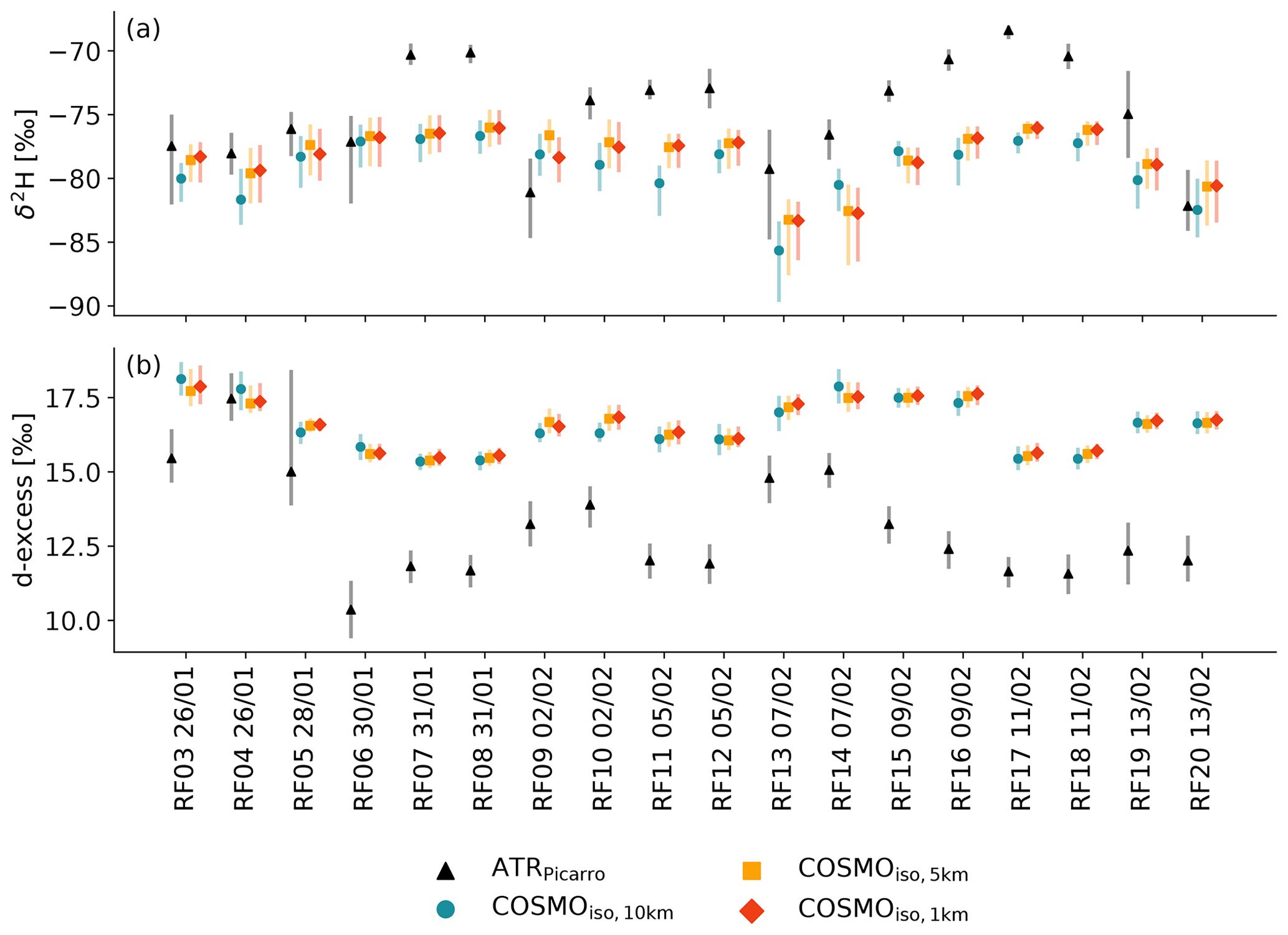
Figure 10 Median (marker) and the 25th to 75th percentile range (transparent line/error bars) of cloud base (a) δ²H and (b) d-excess for each ATR flight. Shown are the observations from the ATR (black) and the simulations COSMO_iso,10 km (teal), COSMO_iso,5 km (orange), and COSMO_iso,1 km (red). For the COSMO_iso simulations, only the data from the hourly time steps that are closest to the ATR flights and only the data in the domain 54.5–61^∘ W and 11–16^∘ N are taken into account.

The (close to) saturated layer extends over ∼ 950–900 hPa in COSMO_iso and over ∼ 950–820 hPa in the measurements from the downward profiles of the ATR, the measurements from the HALO dropsondes, the ERA5 reanalysis, and the ECHAM6-wiso simulation (Fig. 9e). Using high relative humidity (> 80 %) as a proxy for the presence of clouds (since observation-based cloud fraction estimates are only available at cloud base), we conclude that COSMO_iso generally has a shallower cloud layer than the other datasets and presumably has difficulties in producing cloud-top anvils accurately. This behaviour is also observed in other regional model simulations of shallow trade-wind clouds (Beucher et al., 2022, note that they included a shallow convection parameterisation, while we did not). In our COSMO_iso simulations, the rather coarse vertical resolution (Sect. 2) might be a reason for the too shallow representation of clouds.

Compared to the measurements from the downward profiles of the ATR, COSMO_iso has clear cold-dry biases of 1.8–2.1 ^∘C and 1.6–1.7 g kg⁻¹ (Fig. 9a, d and Table 2) in the lower troposphere (from the surface to ∼ 850 hPa). The HALO dropsonde measurements, ERA5, and ECHAM6-wiso (in which the temperature was nudged) match better with the ATR measurements. ECHAM6-wiso even has a weak moist bias in the cloud layer from about 940 to 700 hPa, meaning that COSMO_iso produces its dry-cold bias independently of the ECHAM6-wiso boundary data. Furthermore, the temperature profile of COSMO_iso shows a slightly deeper adiabatic layer (up to 925 hPa; Fig. 9b, c), which suggests a deeper subcloud layer than in the observations, ERA5, or ECHAM6-wiso (cf., Beucher et al., 2022, who found the same in their simulations). The deeper adiabatic layer leads to a more stable cloud layer, with a stronger increase in virtual potential temperature with height (Fig. 9b) in COSMO_iso than in the other datasets. This matches the finding above that COSMO_iso has fewer deep clouds (reaching above 850 hPa).

Table 2 Root-mean-square differences of the median profiles (shown in Fig. 9) of the HALO dropsondes, ERA5, ECHAM6-wiso, COSMO_iso,10 km, COSMO_iso,5 km, and COSMO_iso,1 km data relative to the ones from the ATR_{down profile} data over the layer 1000–850 hPa.

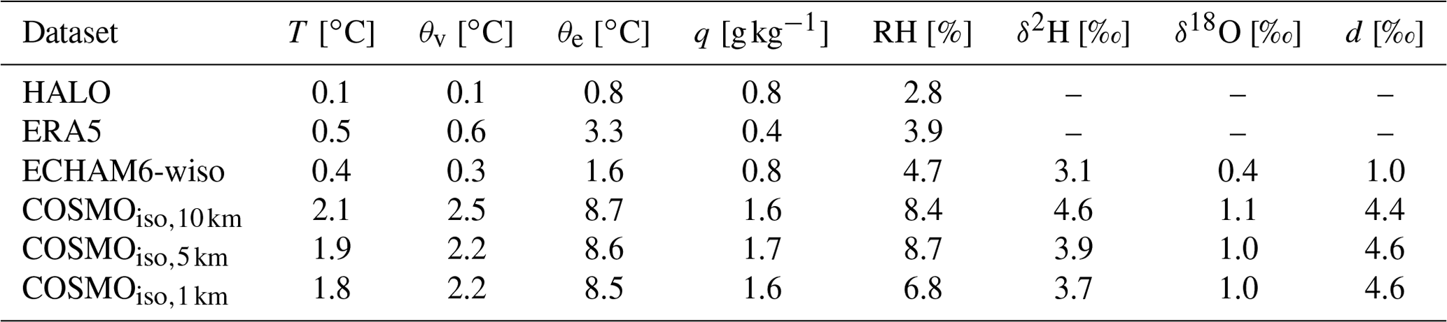
The cold-dry bias in COSMO_iso is associated with slightly too depleted vapour compared to the ATR measurements (Fig. 9f and g and Table 2). In contrast, COSMO_iso produces too enriched vapour in the free troposphere (above ∼ 800 hPa). ECHAM6-wiso shows slightly too enriched vapour in the cloud layer and a more accurate decrease in heavy isotopes above cloud tops compared to the ATR observations than COSMO_iso. The d-excess in vapour (Fig. 9h) is almost constant throughout the vertical column in ECHAM6-wiso and COSMO_iso. While the values in ECHAM6-wiso overlap with the ATR data (at least up to ∼ 750 hPa), COSMO_iso is shifted towards higher values by ∼ 4.5 ‰ (Fig. 9h; the bias is visible up to 200 hPa, not shown). Given the fact that ECHAM6-wiso does not have the same isotope biases as COSMO_iso, it follows that COSMO_iso must produce them within the regional model domain.

The low-level biases in temperature, humidity, and δ²H are physically consistent. Due to the cold bias alone, a dry and a depletion bias can be expected. In fact, about two-thirds of the bias of δ²H and one-fourth of the bias of δ¹⁸O can be explained by the temperature bias (via the temperature-dependency of equilibrium fractionation). This also means that isotopes can only provide limited information about the origin of the low-level biases. Different mechanisms possibly cause some of the identified biases at low levels. (1) An overestimation of the evaporation of hydrometeors would explain a low-level cold bias (Fig. 9a). This, however, would simultaneously lead to a moistening, which is not consistent with the dry bias in the COSMO_iso profiles (Fig. 9d). (2) A too strong convective mixing (across the full depth of the shown profiles), which transports dry-depleted air downward and moist-enriched air upwards, would fit the observed low-level dry-depletion bias but only partly with the conditions in the free troposphere with the too enriched vapour but no moist bias (Fig. 9d, f, g). Moreover, such a mixing process is expected to lead to a low-level warm bias (downward transport of high potential temperature and upward transport of low potential temperature) and not a low-level cold bias, as observed here (Fig. 9a). Lastly, the underestimation of clouds reaching above 900 hPa (Fig. 9e) does not directly support too strong mixing. If convective mixing was too strong, the few higher-reaching clouds in COSMO_iso would need to mix much more efficiently than their more abundant shallow counterparts in the other datasets. (3) Another possible explanation for the cold bias that has not been investigated here but has been found in earlier COSMO evaluation studies (Heim et al., 2021) is too high outgoing long-wave radiation (top-of-the-atmosphere) due to a too dry free-troposphere or too few low-level clouds. However, we do not observe a dry bias in the free troposphere (Fig. 9d). Furthermore, the cloud base cloud fractions of COSMO_iso are rather too high compared to the ATR-based estimates (Fig. 5). (4) Finally, we cannot rule out that the biases are caused by the spectral nudging (horizontal winds above 850 hPa) applied for the simulations (e.g. Wehrli et al., 2018; Sun et al., 2019). However, in another study (Beucher et al., 2022), a cold-dry bias was also found in free-running simulations that were performed without spectral nudging.

Two mechanisms might explain the enrichment bias above 800 hPa (Fig. 9f, g). (1) Too small conversion efficiencies (i.e. too low autoconversion rate within the cloud column) could explain an enrichment bias of about 10 ‰ in δ²H in the cloud-top outflow region of shallow cumulus clouds (see Rayleigh model including precipitation efficiency in Noone, 2012). However, the magnitude of the bias observed here (offset of roughly 60 ‰ for δ²H) is too large to solely be explained by this effect. (2) Another possible explanation is that too strong cloud-top evaporation occurs due to too strong turbulent mixing at the trade inversion. This could lead to only weak moistening but strong enrichment due to close to total (thus non-fractionating) droplet evaporation. The large isotope bias co-located with a very small or inexistent humidity bias in the region of the trade inversion and the level of the deepest cloud tops illustrate that the isotopes contain additional, complementary information for assessing some model biases.

Possible reasons for a d-excess bias (Fig. 9h) are wrong near-surface humidity gradients or the use of inappropriate non-equilibrium fractionation factors. A comparison to ship-based observations from EUREC⁴A (not shown) revealed that, in our case, too low relative humidity with respect to sea surface temperatures accounts for a large part of the identified d-excess bias. Since the sea surface temperatures in COSMO_iso are identical to the ones in ECHAM6-wiso, the too low relative humidity must result from the dry bias discussed above. The remaining share of the d-excess bias might be due to the choice of the non-equilibrium fractionation factor in the model simulations. Evidence is available that the chosen value in COSMO_iso can still be improved compared to observations (Zannoni et al., 2022). The wind-dependent formulation of Merlivat and Jouzel (1979), used in ECHAM6-wiso, and the output from a sensitivity experiment with COSMO_iso with a new wind-dependent formulation of the non-equilibrium fractionation factor from work done by Dütsch (2021, see experimental simulation shown in Supplement 4) yield d-excess values closer to the ATR observations than the evaluated COSMO_iso simulations.

The slightly deeper subcloud layer (adiabatically stratified; Fig. 9b, c) of COSMO_iso in comparison to the ATR and HALO observations, as well as ECHAM6-wiso and ERA5 data, is likely due to too strong turbulent mixing in the subcloud layer and at cloud base. Additionally, the differences in the vertical resolution of the compared datasets could play a role in the observed differences in the profiles. Indeed, ERA5 has roughly twice as many model levels in the layer 1000 to 850 hPa as the three COSMO_iso simulations. However, ECHAM6-wiso has fewer levels in the considered layer. Thus, it is not plausible that the deeper adiabatic layer in COSMO_iso originates only from a vertical resolution effect. The above-stated hypothesis of a too strong turbulent mixing at low levels in the simulations is confirmed by smaller vertical differences between cloud base and subcloud values of humidity, δ²H, and d-excess in COSMO_iso compared to the ATR as shown in Villiger (2022).

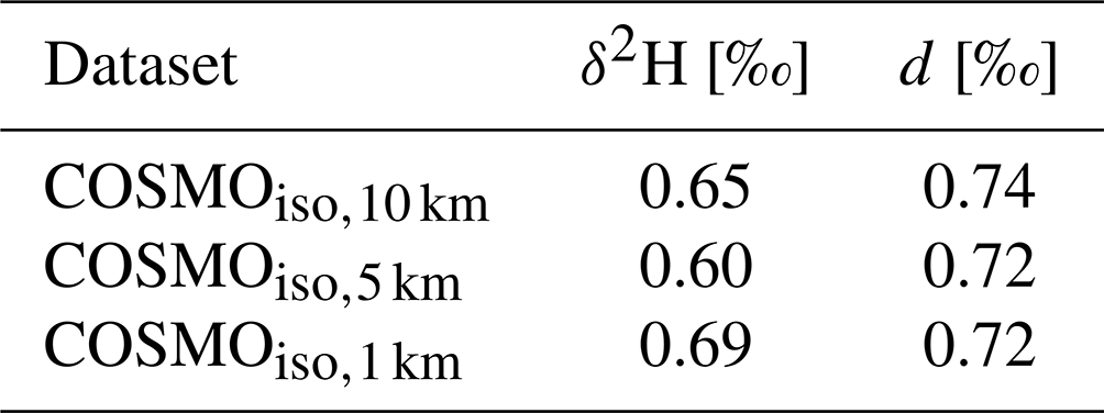
After having discussed various biases, we want to evaluate the development of isotope variables over time. To this end, we focus on cloud base and compare the flight-to-flight variability found in the ATR data to the simulations. High correlations (Table 3) between the two datasets (Fig. 10) suggest that the observed temporal evolution of δ²H and d-excess is well captured by the three COSMO_iso simulations. Another similarity between observations and simulations is that δ²H (Fig. 10a) generally shows a larger in-flight spatial variability at cloud base compared to the flight-to-flight temporal (synoptic) variability. This highlights the importance of mesoscale variability at cloud base, which is the topic of the following section.

Table 3 Pearson correlation coefficients for δ²H in vapour and d-excess in vapour (d) between the median cloud base values from each ATR flight (RF03–RF20) and the hourly median values of all cloud base grid points in the domain 54.5–61^∘ W and 11–16^∘ N that are closest in time to the ATR flights from the three COSMO_iso simulations.

4 Drivers of the horizontal variability of isotopes at cloud base

The detailed examination of the observed and simulated isotope signals at cloud base in the previous section (Fig. 10) showed that δ²H has a large spatial (in-flight) and temporal (flight-to-flight) variability, while the d-excess varies mainly from flight to flight. The flight-to-flight variability is related to the variability of the synoptic circulation. From earlier studies, it is known that the d-excess is negatively correlated with the distance to the moisture source (Aemisegger et al., 2021b), which is closely linked to the prevailing large-scale circulation. However, the drivers behind the mesoscale (in-flight) variability of isotopes at cloud base have not been investigated so far. Here, this topic is addressed by looking at the isotopic characteristics of different environments at cloud base. First, features at the cloud base level are defined in the observational and simulated data based on a case study on 2 February 2020. Second, the whole datasets are used for a statistical description of these features. Based on the findings of Sect. 3, only the data from the COSMO_iso,1 km simulation are considered here. Compared to the lower-resolution COSMO_iso simulations, COSMO_iso,1 km reproduces the spatial cloud patterns, cloud base cloud fraction, and liquid water content better.

4.1 Detailed case study

On 2 February 2020, ATR conducted research flights 9 (RF09) and 10 (RF10) (Bony et al., 2022). Here, we focus on RF10 for an illustrative case study. RF10 included three rectangles at cloud base. During these, the aircraft sampled clear-sky environments at both edges of the rectangle and a Flower cloud in between (Figs. 11a, b and 12e). Beneath the Flower cloud, a cold pool is spreading radially away from the cloud centre (Fig. 11a, b). The edges of the cold pool are clearly marked by shallow clouds arranged in an arc at the edge of a clear-sky patch visible in the satellite image (dashed blue lines in Fig. 11a, b). The ATR cloud base rectangle is positioned such that its southern tip lies inside (or above) the cold pool, while its northern tip lies outside.

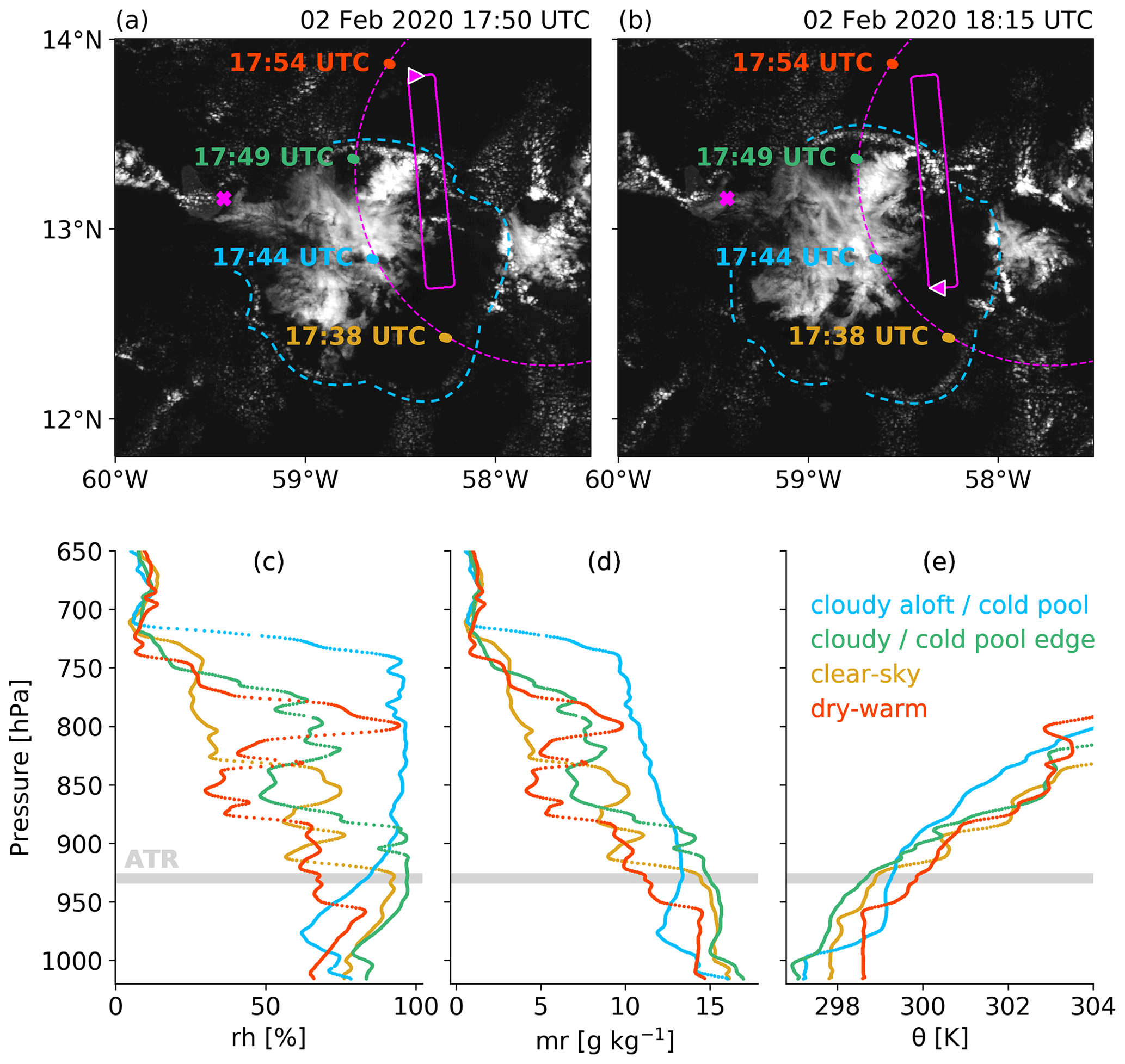
Figure 11 Cloudiness viewed by the visible channel of the GOES-16 satellite on 2 February 2020 together with the cloud base flight track of the ATR during RF10 (continuous pink) and the position of the ATR (pink triangle) at (a) 17:50 UTC and (b) 18:15 UTC (time steps chosen such, that the ATR is located at the northern and southern edge of the cloud base rectangle). The two maps also show the horizontal location of four dropsondes launched from HALO during its circular flight pattern (dashed pink) with the launch time indicated to the left (orange, blue, green, red). The dashed blue lines show the edges of the cold pool spreading radially away from the cloud in the centre of the satellite image. (c–e) Lower-tropospheric profiles of the four HALO dropsondes (shown in panel a, b) displaying (c) relative humidity, (d) mixing ratio, and (e) potential temperature. Note that the x axis of (e) is set such that cloud base differences between the profiles are visible. The profile labels in panel (e) are intended to help the reader link the figure to the text.

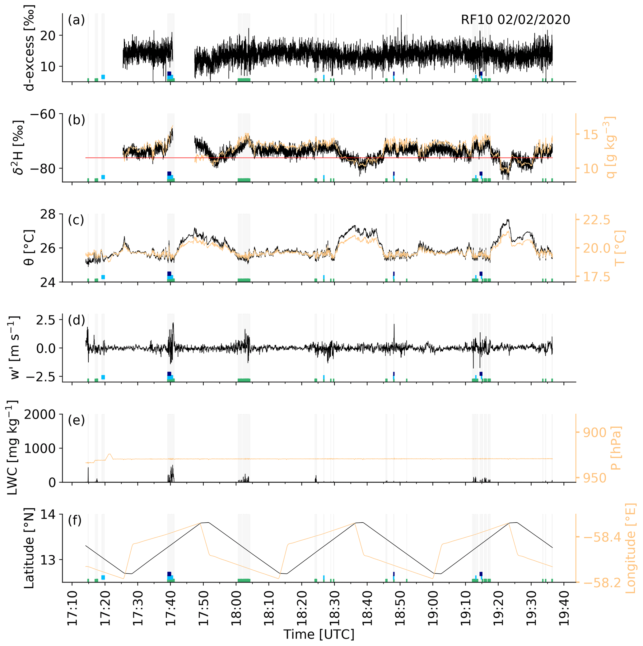
Figure 12 Time series of ATR measurements at cloud base during RF10 on 2 February 2020. Shown are (a) d-excess in vapour, (b) δ²H in vapour (black) and specific humidity (sandy), (c) potential temperature (black) and temperature (sandy), (d) vertical wind velocity fluctuations relative to the flight-segment mean, (e) liquid water content (black) and pressure (sandy), and (f) latitude (black) and longitude (sandy) of the ATR's position. In all panels, the grey shading indicates the presence of liquid water and the green/light-blue/dark-blue bars at the bottom of (a, b, c, d, f) the cloud/drizzle/rain flags from the PMA dataset. Temperatures, vertical velocity, and positional data come from the ATR CORE dataset; d-excess, δ²H, and specific humidity from the ATR Picarro dataset; and liquid water content from the ATR PMA dataset.

The four sondes dropped from HALO in proximity to the flight track of the ATR demonstrate how different the environments in and around the Flower cloud were (note that the snapshots of the satellite images in Fig. 11 do not correspond to the exact launch times of the dropsondes, which require approximately 10 min to reach the surface assuming a launch altitude of 10 km and an average fall speed of 16 m s⁻¹ based on the value range suggested in George et al., 2021a). Looking at the measured profiles from the perspective of the ATR flying at cloud base (∼ 940 hPa; sandy line in Fig. 12e), one can distinguish between a profile with dry-warm conditions at cloud base (red profile in Fig. 11), two profiles with humid-cold conditions at cloud base (orange and green profiles in Fig. 11), and a profile with a deep cloud layer aloft (blue profile in Fig. 11).

The blue profile with the deep cloud layer aloft, near the centre of the Flower cloud, bears the imprint of the cold pool in the subcloud layer. It is characterised by a saturated layer from 900 to 700 hPa (Fig. 11c), which most likely led to the formation of rain (also observed by the ATR; see Fig. 12e). Below the cloud layer, isothermal conditions prevail (Fig. 11e), while relative humidity (Fig. 11c–d) rapidly decreases (promoting the evaporation of falling hydrometeors). At about 975 hPa, relative humidity reaches a local minimum value (Fig. 11c), which is co-located with a temperature drop of about 2 K (Fig. 11e), pointing towards a strong evaporatively triggered cold pool. A similar, although weaker, temperature drop is visible in the green profile, located at the edge of the cold pool. The comparably shallow mixed-layer height in the two (blue and green) soundings matches the definition of cold-pool soundings applied in Touzé-Peiffer et al. (2022).

Although the orange profile is located inside the cold pool (Fig. 11a, b), it does not show the cold-pool characteristic temperature drop near the surface. Possibly, the differences between the green and orange profiles are related to their position relative to the cold-pool centre. Towards the east, where the orange profile is located, the radially spreading cold pool moves against the general flow of the easterlies, seemingly leading to a quick alteration of the air's cold-pool characteristics. Lastly, as expected from its position outside the cold pool (Fig. 11a, b), the red profile is totally unaffected by the cold air spreading near the surface. Instead, it shows an adiabatic profile, typical for the well-mixed subcloud layer.

At the altitude flown by the ATR, the largest horizontal contrasts in humidity and temperature are found between the cloudy (green) and warm clear-sky (red) dropsonde profiles, which match with the observations of the ATR (Fig. 12). In the clear-sky background environments at the northern edge of the rectangle (at 13.8^∘ N; Fig. 12f), specific humidity and δ²H in vapour reach minimum values (Fig. 12b), while a level-relative maximum is reached in temperature (Fig. 12c). On the long side of the rectangle, inside cloudy flight sections (Fig. 12e and grey shadings in all panels), specific humidity and δ²H in vapour are higher, and temperature is lower compared to their respective mean values. Regarding the turbulence intensity indicated by the vertical velocity fluctuations (relative to the flight-segment mean; Fig. 12d), the cloudy sections are quite turbulent with amplitudes of fluctuations up to 2 m s⁻¹, while the clear-sky background environments exhibit weak turbulence close to laminar flow conditions. For the d-excess (Fig. 12a), it is not possible to make a statement about a possible influence of the immediate surroundings (cloud vs. clear-sky) due to the noise of the measurements.

The fact that the clear-sky environment north of the Flower cloud distinguishes itself from the one in the south by lower humidity and higher potential temperature leads to the conclusion that it is a region where air masses subside (see the location of the ATR icon in the schematic Fig. 1a), balancing the upward air mass transport inside the clouds. The clear-sky environment at the southern edge of the cloud base rectangle has no particular anomalies in any observed variables. Possibly, the characteristics of this southern clear-sky environment are shaped by dissipated former clouds (i.e. high humidity; cf., Albright et al., 2022).

Coming back to the original purpose of this section (i.e. to study the in-flight isotope variability at cloud base), the cloud base time series of the ATR (Fig. 12) clearly show that the variability in δ²H in the vapour is driven by the contrast between cloudy and dry-warm, clear-sky background environments. Thus, the question arises whether these patterns are reproduced by the COSMO_iso simulations.

On 2 February 2020 at 15:00 UTC, a large partially precipitating cloud, resembling a Flower cloud, appears in COSMO_iso,1 km just north of the ATR flight track (Fig. 13). The humid environment of the cloud is flanked to the west and east by dry-warm patches (Figs. 13a, b and 14a). These dry-warm blobs are characterised by low δ²H (Figs. 13c and 14b) and low d-excess (Figs. 13d and 14c) in vapour. Thus, COSMO_iso,1 km produces dry-warm features at cloud base, which match the above description based on the ATR and HALO dropsonde observations. Furthermore, it is the contrast between the dry-warm blob and the cloudy environments (Fig. 13c) that shape the width of the distribution of simulated δ²H values, similar to what has been observed in the ATR cloud base measurements.

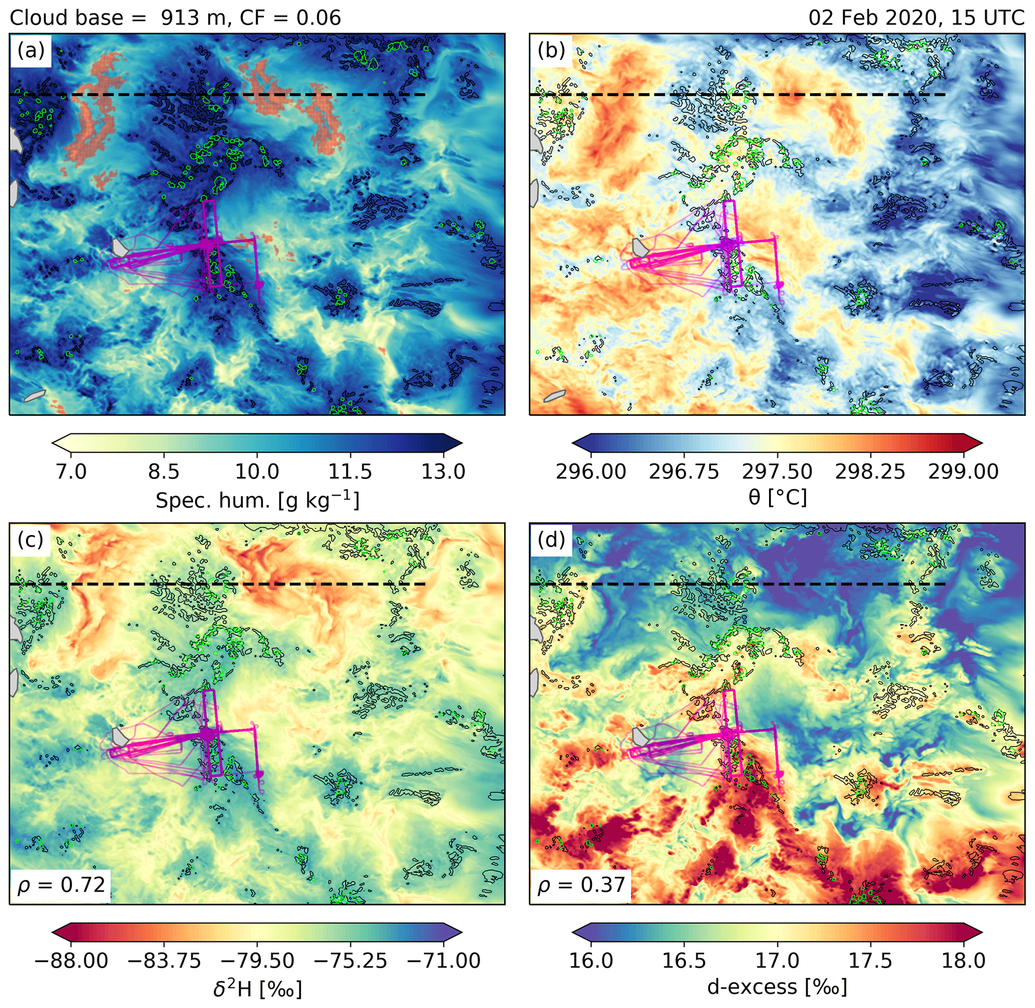
Figure 13 Fields of (a) specific humidity, (b) potential temperature, (c) δ²H in vapour, and (d) d-excess in vapour at cloud base (z= 913 m) in the domain 54.5–61^∘ W and 11–16^∘ N from the COSMO_iso,1 km dataset at 15:00 UTC on 2 February 2020. The transparent red dots in panel (a) show grid points identified as dry-warm (see definition in text); the pink lines represent the track from all ATR flights; and the black line indicates the position of the cross-section shown in Fig. 14. Liquid cloud water contents of 10 mg kg⁻¹ are shown as black contours and rain water contents of 1 mg kg⁻¹ as green contours. In panels (c, d), the Pearson correlation coefficients (ρ) between the cloud base specific humidity and (c) δ²H in vapour, (d) d-excess in vapour are indicated in the lower left corner. The cloud base cloud fraction (CF) at this time and in this region corresponds to 6 %.

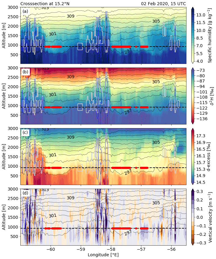
Figure 14 Cross-sections at 15.2^∘ N of (a) specific humidity, (b) δ²H in vapour, (c) d-excess in vapour, and (d) vertical velocity from COSMO_iso,1 km at 15:00 UTC on 2 February 2020. Shown is also potential temperature (black contours), cloud water contents of 10 mg kg⁻¹ (grey contours), rain water contents of 10 mg kg⁻¹ (dashed blue contours) and cloud base height (dashed black line; the level at which the fields are shown in Fig. 13) with the cloud base grid points identified as dry-warm (red dots; less than 0.01^∘ latitude away from the cross-section). The location of the cross-section is indicated in Fig. 13.

Putting these findings into the context of the theory summarised in the Introduction (Sect. 1), it follows that the variability of δ²H at cloud base mirrors the mesoscale transport as cloudy environments are more enriched (updraught of freshly evaporated moisture) compared to dry-warm environments (subsidence of depleted vapour from aloft). This, however, does not mean that microphysical processes do not influence δ²H as well. Depletion of the vapour inside the cloud due to the formation of liquid droplets most likely reduces the observed horizontal contrasts between cloudy and dry-warm environments at cloud base. The imprint of these local processes on δ²H in the vapour is, however, much smaller than the signal of the mesoscale transport that reflects the cloud processing integrated over the mesoscale moisture cycle.

4.2 Statistical evaluation

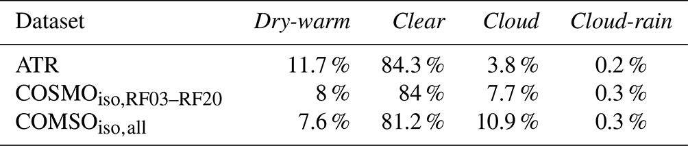
To assess the robustness of the insights gained from the 2 February 2020 case, objective criteria to detect the different cloud base environments in the two datasets are introduced. For the ATR, the flags from the PMA dataset (Bony et al., 2022) are used to distinguish between time steps in clear-sky conditions and time steps with liquid water droplets in the surroundings. The following categories are defined (see the percentage of data points in each category in Table 4):

• clear, indicating time steps with no PMA flags;

• cloud, indicating time steps with the PMA flags of clouds but no rain nor drizzle;

• cloud-rain, indicating time steps with the PMA flags of clouds and rain.

Note that the PMA flags indicate rain but no clouds for 1.3 % of the time (compared to 0.2 % indicating rain and clouds). These time steps are excluded from the categorisation because they complicate the interpretation of the isotope signal (highly depending on the formation altitude of the rain). The time steps identified as clear are relabelled as dry-warm if they have a negative anomaly in specific humidity (q) and a positive anomaly in potential temperature (θ). The anomalies are defined relative to each flight's mean $\stackrel{\mathrm{‾}}{X}$ and standard deviation σ(X) of the respective variable X at cloud base with the criteria $q<\stackrel{\mathrm{‾}}{q}-\mathit{\sigma }\left(q\right)$ and $\mathit{\theta }>\stackrel{\mathrm{‾}}{\mathit{\theta }}+\mathit{\sigma }\left(\mathit{\theta }\right)$ (e.g. red lines in Fig. 12b, c), which must be fulfilled for a time step to be assigned to the dry-warm category. The two categories clear and dry-warm are exclusive (i.e. data points identified as dry-warm are removed from the clear category).

Table 4 Percentage of data points assigned to one of the four cloud base categories (dry-warm, clear, cloud, cloud-rain). For the ATR, the time steps with valid isotope data are taken into account (RF03–RF20; note that these are fewer data points than available in the PMA dataset alone, because the isotope dataset has data gaps due to calibration or instrument failure, especially during rainy flight segments). For COSMO_iso,1 km, the data in the domain 54.5–61^∘ W and 11–16^∘ N are taken into account; once only from the hourly time steps that are closest to the ATR flights (COSMO_{iso,RF03–RF20}) and once for all simulated time steps (COMSO_iso,all).

For the COSMO_iso,1 km data, the cloud base grid points in the evaluation domain 54.5–61^∘ W and 11–16^∘ N are stratified according to their cloud and rain water contents:

• clear, representing grid points with cloud water content below 10 mg kg⁻¹ and rain water content below 1 mg kg⁻¹;

• cloud, representing grid points with cloud water content exceeding 10 mg kg⁻¹ (black contours in Fig. 13) and rain water content below 1 mg kg⁻¹;

• cloud-rain, representing grid points with cloud water content exceeding 10 mg kg⁻¹ (black contours in Fig. 13) and rain water content exceeding 1 mg kg⁻¹ (green contours in Fig. 13).

From the clear category, the grid points with a negative anomaly in q and a positive anomaly in θ are reassigned to the dry-warm category, similarly as it is done for the measurements. Here, the anomalies are defined grid-point-wise, by removing the daily cycle. The hour-of-the-day mean and standard deviation for each grid point are calculated over the whole simulated period (20 January to 13 February 2020). Note that for the ATR observations, the effect of the daily cycle could not be subtracted because too few observations are available, in particular at night, preventing a robust estimation of the daily cycle. Dry-warm grid points are then selected using the following criteria: $q_{i,t}<\stackrel{\mathrm{‾}}{q_{i,\mathrm{h}\left(t\right)}}-\mathit{\sigma }\left(q_{i,\mathrm{h}\left(t\right)}\right)$ and ${\mathit{\theta }}_{i,t}>\stackrel{\mathrm{‾}}{{\mathit{\theta }}_{i,\mathrm{h}\left(t\right)}}+\mathit{\sigma }\left({\mathit{\theta }}_{i,\mathrm{h}\left(t\right)}\right)$ (where i indicates the grid points in the evaluation domain, t the hourly time steps of the simulated period, and h(t) the hour of the day corresponding to time step t). An overview of the number of identified dry-warm grid points per time step is given in Supplement 3, and for the case study on 2 February 2020 the dry-warm grid points are shown as red dots in Fig. 13a. The grid points with rain water content exceeding 1 mg kg⁻¹ but remaining below the cloud water content threshold of 10 mg kg⁻¹ are not assigned to any category. Such grid points make up 0.6 % of the cloud base grid points over the hourly time steps closest to the ATR flights (compared to 0.3 % with rain and clouds).

Applying the above-described categorisation to the full ATR and COSMO_iso,1 km datasets yields similar gradients in the cloud base environments (Fig. 15) as observed on 2 February 2020 (Figs. 12, 13, and 14). Both datasets describe a gradient from dry-depleted to moist-enriched conditions, going from dry-warm to cloud/cloud-rain environments (Fig. 15a, b). The specific-humidity anomalies of the different cloud base environments are comparable in the ATR and the COSMO_iso data (Table 5). The δ²H anomalies are comparable for the dry-warm category. The cloud and cloud-rain environments, however, are more enriched relative to the level mean in the ATR data than in the COSMO_iso data.

Table 5 Median values of the cloud base anomalies in specific humidity (q), δ²H in vapour, and d-excess (d) in vapour for the data points identified as dry-warm, clear, cloud, cloud-rain (see the text for the definition) and the difference between the median of the cloud-rain and the dry-warm grid points (calculated with the exact values and not the rounded medians shown here) from the ATR and COSMO_iso,1 km. For the ATR data, anomalies are defined relative to each flight's mean cloud base conditions. For COSMO_iso,1 km, anomalies are defined relative to each time step's hour-of-the-day average cloud base conditions in the domain 54.5–61^∘ W and 11–16^∘ N. Shown are the median values over the cloud base time steps of the ATR (RF03–RF20), the COSMO_iso,1 km cloud base grid points at the hourly time steps that are closest to the ATR flights (COSMO_{iso,RF03–RF20}) and over the whole simulated period (20 January to 13 February 2020; COSMO_iso,all). Note that the 25th, 50th, and 75th percentiles of these variables in each cloud base environment are shown in Fig. 15.

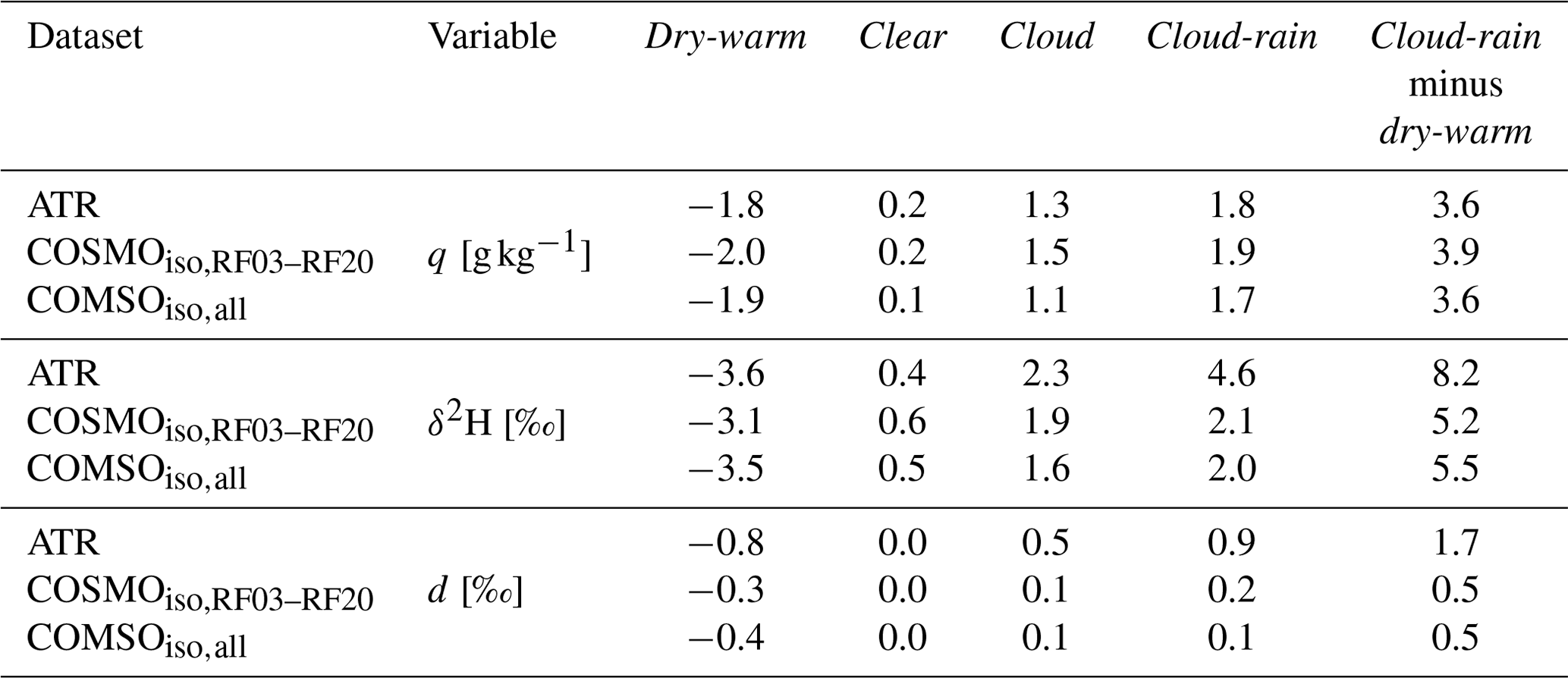
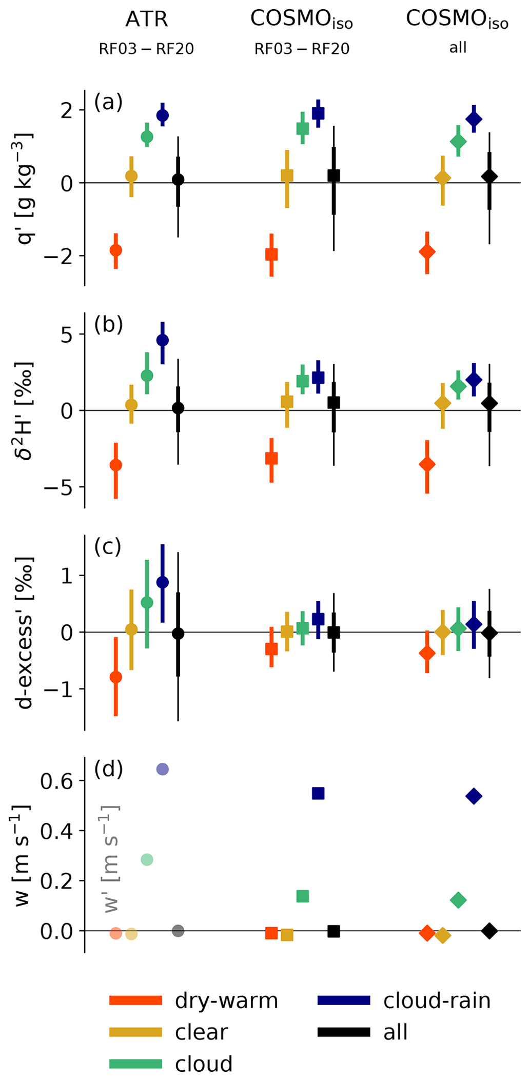
Figure 15 Distributions of the cloud base anomalies in (a) specific humidity, (b) δ²H in vapour, and (c) d-excess in vapour of the data points identified as dry-warm, clear, cloud, cloud-rain (see the text for the definition) and all of them together (black). For the ATR data, anomalies are defined relative to each flight's mean cloud base conditions. For COSMO_iso,1 km, anomalies are defined relative to each time step's mean cloud base conditions in the domain 54.5–61^∘ W and 11–16^∘ N. Shown are the median (markers), the 25th to 75th percentile range (lines), and for the overall distribution (black) the 10th to 90th percentile range (thin black line) of the cloud base data points collected by the ATR (RF03–RF20) and the COSMO_iso,1 km cloud base grid points at the hourly time steps that are closest to the ATR flights (COSMO_{iso,RF03–RF20}) and over the whole simulated period (20 January to 13 February 2020; COSMO_iso,all). (d) The mean absolute vertical velocity w for COSMO_iso and mean vertical velocity fluctuations w^′ for the ATR (see text for the reasoning behind the variable choice) at cloud base. For the ATR, only RF10–RF19 provide vertical velocity measurements and are included here. Table 4 gives the percentage of data points in each category and Table 5 gives the numerical values of the median anomalies. Supplement 3 provides alternative versions of this figure.

Due to the chosen statistical approach, we can now also identify contrasts in the d-excess at cloud base with negative anomalies in the dry-warm blobs and positive anomalies inside clouds (Fig. 15c). However, the d-excess distributions of the different cloud base environments overlap a lot, both in the ATR data and the simulations (especially if the full width of the distribution is considered as in Supplement 3). The direction of the observed d-excess gradients does not fit the general expectations of high d-excess being associated with low relative humidity and vice versa (Bony et al., 2008). Looking at the vertical sections on 2 February 2020 (Fig. 14c), one notes that d-excess is high near the surface, where ocean water is evaporated under non-equilibrium conditions (Aemisegger and Sjolte, 2018), and slightly decreases with altitude due to shallow cloud processing (Thurnherr et al., 2021). Inside the lower part of the clouds, however, d-excess remains high, especially in the vicinity of strong updraughts (Fig. 14d). Additionally, as d-excess is higher below precipitating clouds (Fig. 14c at about −60.5 and −58.2^∘ E) than below non-precipitating clouds (Fig. 14c at about −55.9^∘ E), partial evaporation of falling hydrometeors may additionally increase the d-excess in the subcloud layer vapour, which is then transported to cloud base in convective updraughts. In other words, the observed contrasts in d-excess between cloudy and dry-warm environments at cloud base, similar to q and δ²H, reflect mesoscale transport as well as the microphysical processes embedded in this flow.

The full distribution width of cloud base anomalies (black in Fig. 15) is explained by the contrast between the different cloud base environments. In the case of specific humidity and δ²H, the dry-warm and cloud-rain categories are centred (median value) outside the interquartile range of the full distribution, while it is the other way around for the d-excess. This applies to both datasets, the observations and the simulations. It means that the d-excess is not as strongly influenced by the mesoscale circulation associated with clouds as δ²H and specific humidity. Other factors (e.g. spatial gradients as in Fig. 13d) play an equally or even larger role in the formation of d-excess anomalies.

We have a look at the mean vertical velocity (fluctuations; in case of the ATR data) inside the different cloud base environments to support the assumption that the dry-warm and cloud/cloud-rain categories represent different branches of the mesoscale overturning circulation (Fig. 15d). In the COSMO_iso,1 km data, the mean vertical velocity is negative in the dry-warm and clear environments and positive in the cloud and cloud-rain environments, as we would expect from an overturning circulation. Similar contrasts between the cloud base environments are found in the ATR data for the mean vertical velocity fluctuations. Note that for the ATR data we look at fluctuations relative to the flight-segment mean, because the accuracy of 0.1 m s⁻¹ of the aircraft's vertical motion measurements is not sufficient for estimating mean vertical winds (Lenschow et al., 2007).

5 Summary and conclusion

A combination of observational data from EUREC⁴A was used to evaluate COSMO_iso simulations at different horizontal resolutions with a focus on processes at cloud base, which is the rooting level for cloud formation. This is the first isotope-enabled modelling study of shallow cumulus clouds in the trades with a storm-resolving model and in real large-scale meteorological conditions (i.e. applying a spectral nudging of the free-tropospheric horizontal winds). The detailed process-based evaluation focusing on shallow clouds was only possible thanks to the novel and unique observations collected during EUREC⁴A, in particular on board the French ATR-42 aircraft.

The comparison to satellite images showed that COSMO_iso is capable of distinguishing between Fish clouds, Flower clouds, and more finely structured cloud patterns, such as Gravel and Sugar clouds. Overall, if the model resolution is high, the simulated mesoscale cloud organisation agrees better with the satellite images than for simulations with lower resolution. The model differentiates between periods with high-intensity (20–24 January and 6–13 February 2020) and low-intensity rainfall (period in between), which are evident in satellite-based observations. For the major part of the simulated period, the model output matches the diel cycle of the satellite-based precipitation product and earlier studies (Vial et al., 2019). The flight-to-flight and the in-flight variabilities of the isotope signals at cloud base are well captured by the model (similar to earlier studies looking at the meso- to synoptic-scale variability in humidity and isotope variables; Dahinden et al., 2021; de Vries et al., 2022).

However, for some variables, COSMO_iso has important biases. The liquid water content and cloud fraction at cloud base are overestimated but approach the observed values at higher spatial model resolution (for cloud fraction, this behaviour is expected and in agreement with earlier studies, i.e. Heim et al., 2021). Precipitation is spatially more concentrated in the simulations than in the satellite product. This local concentration of precipitation increases with higher model resolution. We find biases in humidity, temperature, and water vapour isotopes in all three simulations. COSMO_iso produces a distinct cold-dry bias at low levels that is consistently associated with too depleted vapour and too high values of the secondary isotope variable d-excess. A cold-dry bias was previously observed in other regional models such as HARMONIE (Gheylla, 2023, humidity bias of similar magnitude; smaller bias in temperature) and AROME (Beucher et al., 2022, both biases of smaller magnitude), while too depleted vapour near the surface was found in COSMO_iso simulations performed by Thurnherr et al. (2021, bias of approx. 2 ‰–4 ‰) over the Southern Ocean. Furthermore, COSMO_iso shows too enriched vapour above the inversion (in agreement with Dahinden et al., 2021; de Vries et al., 2022) but no moist bias. This shows the additional value of isotope observations compared to specific humidity alone and hints towards a misrepresentation of cloud-top processes and their interaction with the dry free troposphere in the model. Different mechanisms that may cause individual biases were discussed and lead to the following recommendations for future research.

We recommend testing the role of turbulent mixing by adjusting the mixing length of the turbulence scheme. Mixing processes in the subcloud layer and at cloud base could be further investigated by combining turbulence and isotope observations from the ATR or by investigating the three-dimensional fields of total kinetic energy in the COSMO_iso,1 km data. The role of the fixed cloud droplet number, which is large compared to the observed spectrum, for the spatial distribution of cloud and rainwater should be assessed. Cloud-top processes in the COSMO_iso data could be investigated in more detail since near the trade inversion isotopes might provide interesting additional information compared to specific humidity alone (formation of the stratiform outflow and sublimation of cloud droplets). Furthermore, we suggest repeating the simulations without applying spectral nudging to assess its potential role in the formation of the low-level cold-dry and depletion bias.

The motivation for the evaluation of the three COSMO_iso simulations was to assess whether they can be used to study the role of the atmospheric circulation at different scales for controlling the formation of shallow cumulus clouds in the trades using isotopes. The realistic representation of cloud organisation patterns, cloud fraction, and precipitation regimes and the temporal evolution of isotope variables at cloud base suggest that COSMO_iso,1 km can serve this purpose, while the simulations with coarser resolution are still useful for looking at the role of the larger-scale circulation as a driver for shallow cloud organisation. The identified model biases in humidity, temperature, and isotope signals in vapour are of minor concern because they can be eliminated by looking at anomalies, as shown in the feature-based evaluation (distinguishing between different environments named dry-warm, clear, cloud, and cloud-rain) of COSMO_iso,1 km. The feature-based evaluation revealed that the low-level biases in the COSMO_iso simulations discussed above are not feature-specific but apply to all the different cloud base environments (cf. Supplement 3). In other words, the processes linked to the formation of these features are accurately reproduced by COSMO_iso.

The investigation of the isotope variability at cloud base identified mesoscale transport (overturning circulation associated with clouds) and not local microphysical processes as the main control of δ²H. The heaviest vapour with the highest d-excess was found inside clouds (directly linked to shallow convective upward transport and partial evaporation of falling hydrometeors), and the lightest vapour with the lowest d-excess was found inside dry-warm, clear-sky environments (directly linked to mesoscale subsidence), in the observations as well as in the COSMO_iso,1 km data. The clear relation between isotope signals and cloud base features reflecting the mesoscale circulation prompts the question whether isotope signals at cloud base contain information on the strength of the cloud-relative overturning circulation. This question is addressed in the second part of this study by adopting a Lagrangian perspective.