Boundary of nighttime ozone chemical equilibrium in the mesopause region: long-term evolution determined using 20-year satellite observations

The assumption of nighttime ozone chemical equilibrium (NOCE) is widely employed for retrieving the O_x-HO_x components in the mesopause from rocket and satellite measurements. In this work, the recently developed analytical criterion of determining the NOCE boundary is used (i) to study the connection of this boundary with O and H spatiotemporal variability based on 3D modeling of chemical transport and (ii) to retrieve and analyze the spatiotemporal evolution of the NOCE boundary in 2002–2021 from the SABER/TIMED dataset. It was revealed, first, that the NOCE boundary reproduces well the transition zone dividing deep and weak photochemical oscillations of O and H caused by the diurnal variations of solar radiation. Second, the NOCE boundary is sensitive to sporadic abrupt changes in the middle-atmosphere dynamics, in particular due to powerful sudden stratospheric warmings leading to the events of an elevated (up to ∼ 80 km) stratopause, which took place in January–March 2004, 2006, 2009, 2010, 2012, 2013, 2018, and 2019. Third, the space–time evolution of this characteristic expressed via pressure altitude contains a clear signal of an 11-year solar cycle in the 55^∘ S–55^∘ N range. In particular, the mean annual NOCE boundary averaged in this range of latitudes anticorrelates well with the F_10.7 index with the coefficient of −0.95. Moreover, it shows a weak linear trend of 56.2±42.2 m per decade.

1 Introduction

The mesopause (80–100 km) is an interesting region of the Earth's atmosphere possessing quite a number of unique phenomena and processes which can be considered as sensitive indicators/predictors of global climate change and anthropogenic influences on atmospheric composition (e.g., Thomas et al., 1989). Here, the summer temperature at middle and high latitudes reaches its lowest values (down to 100 K (Schmidlin, 1992)). The temperatures below 150 K lead to water vapor condensation and formation of the highest-altitude clouds in the Earth's atmosphere, the so-called “polar mesospheric clouds” or “noctilucent clouds” consisting primarily of water ice (Thomas, 1991). In turn, the temperature of the winter mesopause is essentially higher, so there is a strong negative temperature gradient between the summer and winter hemispheres. At these altitudes, atmospheric waves of various spatiotemporal scales are observed, in particular internal gravity waves coming from the lower atmosphere. Destruction of gravity waves leads to strong turbulence that affects the atmospheric circulation and ultimately manifests itself in the mentioned temperature structure of this region.

Many layer phenomena in the mesopause are related to the photochemistry of the O_x-HO_x components (O, O₃, H, OH, and HO₂). There is a narrow (in height) transition region where photochemistry behavior transforms rapidly from “deep” diurnal oscillations, when the difference between daytime and nighttime values of the O_x-HO_x components can reach several orders of magnitude, to weak photochemical oscillations. As a result, above this region, O and H accumulate to form the corresponding layers. This layer formation manifests itself in the appearance of a secondary ozone maximum and airglow layers of OH and O excited states. Thus, O_x-HO_x photochemistry in the mesopause is responsible for the presence of important (first of all, from a practical point of view) indicators observed in the visible and infrared ranges, which are widely used for ground-based and satellite monitoring of climate changes and wave activity. Moreover, O_x-HO_x photochemistry provides the total chemical heating rate of this region, influences the radiative cooling and other useful airglows (for example, by O₂ excited states), and is involved in the plasma-chemical reactions and formation of layers of the ionosphere. The mentioned transformation of O_x-HO_x behavior with height may occur via the nonlinear response of O_x-HO_x photochemistry to the diurnal variations of solar radiation in the form of subharmonic (with periods of 2, 3, 4, and more days) or chaotic oscillations (e.g., Sonnemann and Fichtelmann, 1997; Feigin et al., 1998). This unique phenomenon was predicted many years ago (Sonnemann and Fichtelmann, 1987) and investigated theoretically by models taking into account different transport processes (Sonnemann and Feigin, 1999; Sonnemann et al., 1999; Sonnemann and Grygalashvyly, 2005; Kulikov and Feigin, 2005; Kulikov, 2007; Kulikov et al., 2020). It was revealed, in particular, that the nonlinear response is controlled by vertical eddy diffusion (Sonnemann and Feigin, 1999; Sonnemann et al., 1999), so 2 d oscillations can only survive at real diffusion coefficients, but the eddy diffusion in the zonal direction leads to the appearance of the so-called reaction–diffusion waves in the form of propagating phase fronts of 2 d oscillations (Kulikov and Feigin, 2005; Kulikov et al., 2020). Recently, the satellite data processing revealed the first evidence of the existence of 2 d photochemical oscillations in the real mesopause (Kulikov et al., 2021).

While regular remote sensing measurements of most O_x-HO_x components are still limited, the indirect methods based on the physicochemical assumptions are useful tools for monitoring these trace gases. In many papers, O and H distributions were retrieved from the daytime and nighttime rocket and satellite measurements of the ozone and the volume emission rates of OH(ν), O(¹S), and O₂(a¹Δ_g) (Good, 1976; Pendleton et al., 1983; McDade et al., 1985; McDade and Llewellyn, 1988; Evans et al., 1988; Thomas, 1990; Llewellyn et al., 1993; Llewellyn and McDade, 1996; Mlynczak et al., 2007, 2013a, 2013b, 2014, 2018; Smith et al., 2010; Xu et al., 2012; Siskind et al., 2008, 2015). The retrieval technique is based on the assumption of ozone photochemical/chemical equilibrium and a physicochemical model of the corresponding airglow, which describe the relationship between local O and H values and measurement data.

The daytime photochemical ozone equilibrium is a good approximation everywhere in the mesosphere and lower thermosphere (MLT) region (Kulikov et al., 2017) due to ozone photodissociation, whereas the applicability of the assumption of nighttime ozone chemical equilibrium (NOCE) is limited: there is an altitude boundary above which NOCE is satisfied to an accuracy better than 10 %. Below this boundary, the ozone equilibrium is disturbed essentially and cannot be used. Good (1976) supposed that NOCE is fulfilled above 60 km, whereas other papers apply the NOCE starting from 80 km, independent of latitude and season. However, studies of NOCE within the framework of the 3D chemical transport models (Belikovich et al., 2018; Kulikov et al., 2018a) revealed that the NOCE boundary varies within the range 81–87 km, depending on latitude and season. In view of the practical need to determine the local altitude position of this boundary, Kulikov et al. (2018a) presented a simple criterion determining the equilibrium boundary using only the data provided by the SABER (Sounding of the Atmosphere using Broadband Emission Radiometry) instrument aboard the TIMED (Thermosphere Ionosphere Mesosphere Energetics and Dynamics) satellite. Making use of this criterion, Kulikov et al. (2019) retrieved the annual evolution of the NOCE boundary from the SABER data. It was revealed that a 2-month averaged NOCE boundary essentially depends on season and latitude and can rise up to ∼ 86 km. Moreover, the analysis of the NOCE boundary in 2003–2005 showed that this characteristic was sensitive to unusual dynamics of stratospheric polar vortex during the 2004 Arctic winter, which was named a remarkable winter in the 50-year record of meteorological analyses (Manney et al., 2005). Moreover, Belikovich et al. (2018) found by a 3D simulation that the excited OH layer repeats well spatiotemporal variability of the NOCE boundary. These results allowed us to speculate that the NOCE boundary can be considered as an important indicator of mesopause processes.

The main goals of this paper are (1) to investigate the relationship between the NOCE boundary according to the mentioned criterion and O and H variability with the use of the 3D chemical transport model and (2) to retrieve and analyze the spatiotemporal evolution of the NOCE boundary in 2002–2021 from the SABER/TIMED dataset. In the next section, we present the used model. In Sect. 3, we briefly describe the criterion of determining the NOCE boundary local height and study how this height is related to the features of O and H distributions from the 3D model. Section 4 explains the methodology of determining the NOCE boundary from satellite data. Section 5 presents the main results obtained from SABER/TIMED data discussed in Sect. 6.

2 The 3D model

We use the 3D chemical transport model of the middle atmosphere developed by the Leibniz Institute of Atmospheric Physics (Sonnemann et al., 1998; Körner and Sonnemann, 2001; Grygalashvyly et al., 2009; Hartogh et al., 2004, 2011). The three-dimensional fields of temperature and winds were adopted by Kulikov et al. (2018b) from the Canadian Middle Atmosphere Model (Scinocca et al., 2008) for the year 2000 with an updated frequency of 6 h. To exclude unrealistic jumps in the evolution of calculated chemical characteristics, linear smoothing between two subsequent updates of these parameters is applied. The model takes into account 3D advective transport and vertical diffusive transport (both turbulent and molecular). The Walcek-scheme (Walcek, 2000) and the implicit Thomas algorithm (Morton and Mayers, 2005) are used for advective and diffusive transport, respectively. The model grid includes 118 pressure-height levels (from the ground to ∼ 135 km), as well as 32 and 64 levels in latitude and longitude, respectively. The chemical part considers 22 constituents (O, O(¹D), O₃, H, OH, HO₂, H₂O₂, H₂O, N, NO, NO₂, NO₃, N₂O, CH₄, CH₂, CH₃, CH₃O₂, CH₃O, CH₂O, CHO, CO, CO₂), 54 two- and three-body reactions, and 15 photo-dissociation reactions. The model uses pre-calculated dependences of dissociation rates on altitude and solar zenith angle (Kremp et al., 1999). The chemistry is calculated by the Shimazaki scheme (Shimazaki, 1985) for the integration time of 9 s.

3 The NOCE criterion

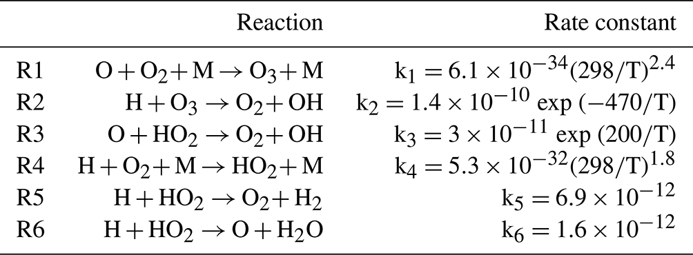
The nighttime ozone chemistry at the mesopause heights is determined mainly by two Reactions (R1–R2) (e.g., Allen et al., 1984); see Table 1. The secondary ozone loss via the O + O₃→2 O₂ reaction becomes important above ∼ 95 km (Smith et al., 2009). Kulikov et al. (2023) verified with simulated and measured data that this reaction does not influence the NOCE boundary determination and may be skipped. Thus, the ozone equilibrium concentration (O${}_{\mathrm{3}}^{\mathrm{eq}})$ corresponding to the instantaneous balance between the production and loss terms is as follows:

$$\begin{array}{}\text{(1)}& {\mathrm{O}}_{\mathrm{3}}^{\mathrm{eq}}={\displaystyle \frac{k_{\mathrm{1}}\cdot \mathrm{O}\cdot {\mathrm{O}}_{\mathrm{2}}\cdot \mathrm{M}}{k_{\mathrm{2}}\cdot \mathrm{H}}},\end{array}$$

where M is air concentration, and k_1-2 represents the corresponding rate constants of the reactions (see Table 1).

Table 1 List of reactions with corresponding reaction rates (for three-body reactions [cm⁶ molecule⁻² s⁻¹] and for two-body reactions [cm³ molecule⁻¹ s⁻¹]) taken from Burkholder et al. (2020).

As mentioned above, the NOCE criterion was developed in Kulikov et al. (2018a). The main idea is that the local values of O₃ and O${}_{\mathrm{3}}^{\mathrm{eq}}$ are close (O${}_{\mathrm{3}}\left(t\right)\approx {\mathrm{O}}_{\mathrm{3}}^{\mathrm{eq}}\left(t\right)$) when ${\mathit{\tau }}_{{\mathrm{O}}_{\mathrm{3}}}\ll {\mathit{\tau }}_{{\mathrm{O}}_{\mathrm{3}}^{\mathrm{eq}}}$, where ${\mathit{\tau }}_{{\mathrm{O}}_{\mathrm{3}}}$ is the ozone lifetime and ${\mathit{\tau }}_{{\mathrm{O}}_{\mathrm{3}}^{\mathrm{eq}}}$ is the local timescale of O${}_{\mathrm{3}}^{\mathrm{eq}}$:

$$\begin{array}{}\text{(2)}& {\mathit{\tau }}_{{\mathrm{O}}_{\mathrm{3}}}={\displaystyle \frac{\mathrm{1}}{k_{\mathrm{2}}\cdot \mathrm{H}}},\end{array}$$

$$\begin{array}{}\text{(3)}& {\mathit{\tau }}_{{\mathrm{O}}_{\mathrm{3}}^{\mathrm{eq}}}\equiv {\displaystyle \frac{{\mathrm{O}}_{\mathrm{3}}^{\mathrm{eq}}}{\left|{\mathrm{dO}}_{\mathrm{3}}^{\mathrm{eq}}/\mathrm{d}t\right|}}={\displaystyle \frac{\mathrm{O}}{\mathrm{H}\cdot \left|\frac{\mathrm{d}}{\mathrm{d}t}\left(\frac{\mathrm{O}}{\mathrm{H}}\right)\right|}}.\end{array}$$

As shown in Kulikov et al. (2018a), ${\mathit{\tau }}_{{\mathrm{O}}_{\mathrm{3}}^{\mathrm{eq}}}$ can be determined from a simplified photochemical model describing the O_x-HO_x evolution in the mesopause region (Feigin et al., 1998), so the criterion of the NOCE validity can be written in the following form:

$$\begin{array}{}\text{(4)}& \begin{array}{rl}\mathrm{Cr}& ={\displaystyle \frac{{\mathit{\tau }}_{{\mathrm{O}}_{\mathrm{3}}}}{{\mathit{\tau }}_{{\mathrm{O}}_{\mathrm{3}}^{\mathrm{eq}}}}}=\mathrm{2}{\displaystyle \frac{k_{\mathrm{1}}\cdot k_{\mathrm{4}}\cdot {\mathrm{O}}_{\mathrm{2}}^{\mathrm{2}}\cdot \mathrm{M}\mathrm{2}}{k_{\mathrm{2}}}}\left(\mathrm{1}-{\displaystyle \frac{k_{\mathrm{5}}+k_{\mathrm{6}}}{k_{\mathrm{3}}}}\right)\\ & \cdot {\displaystyle \frac{\mathrm{1}}{k_{\mathrm{2}}\cdot \mathrm{H}\cdot {\mathrm{O}}_{\mathrm{3}}}}\ll \mathrm{1},\end{array}\end{array}$$

where k_i represents the corresponding reaction constants from Table 1. Calculations with the global 3D chemical transport model of the middle atmosphere showed (Kulikov et al., 2018a) that the criterion ${\mathit{\tau }}_{{\mathrm{O}}_{\mathrm{3}}}/{\mathit{\tau }}_{{\mathrm{O}}_{\mathrm{3}}^{\mathrm{eq}}}\le \mathrm{1}$ defines well the boundary of the area where $\left|{\mathrm{O}}_{\mathrm{3}}/{\mathrm{O}}_{\mathrm{3}}^{\mathrm{eq}}-\mathrm{1}\right|\le \mathrm{0.1}$.

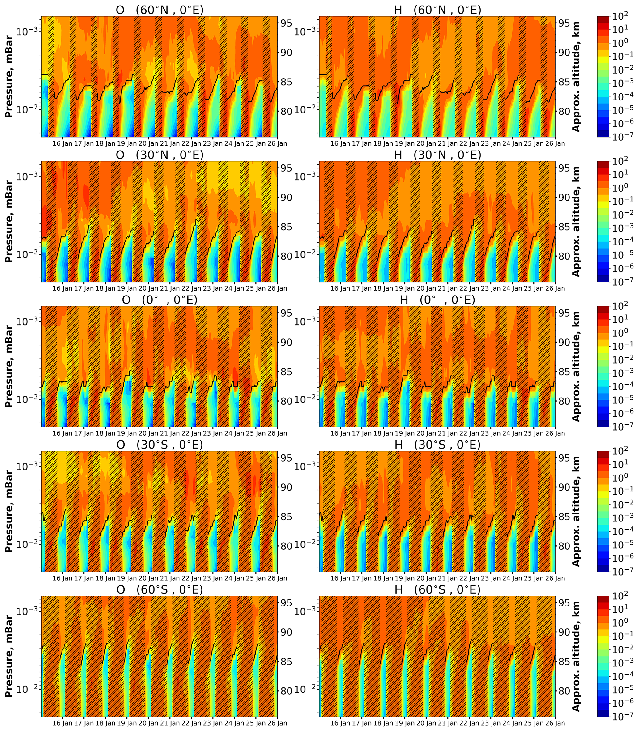
Figure 1 O and H time–height variations above different points in January 2000 calculated by a 3D chemical transport model of the middle atmosphere. Concentrations are normalized by mean daily values, correspondingly, calculated as a function of altitude. Dark bars mark daytime; light bars mark nighttime. Black lines point out the NOCE boundary altitude in accordance with Criterion (5) (Cr=0.1).

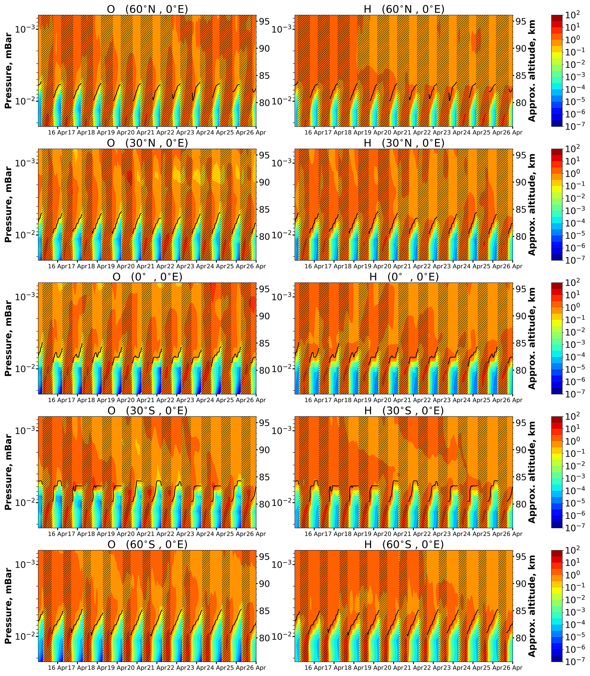
Figure 2 The same as in Fig. 1 but in April 2000. Black lines point NOCE boundary altitude according to Criterion (5) (Cr=0.1).

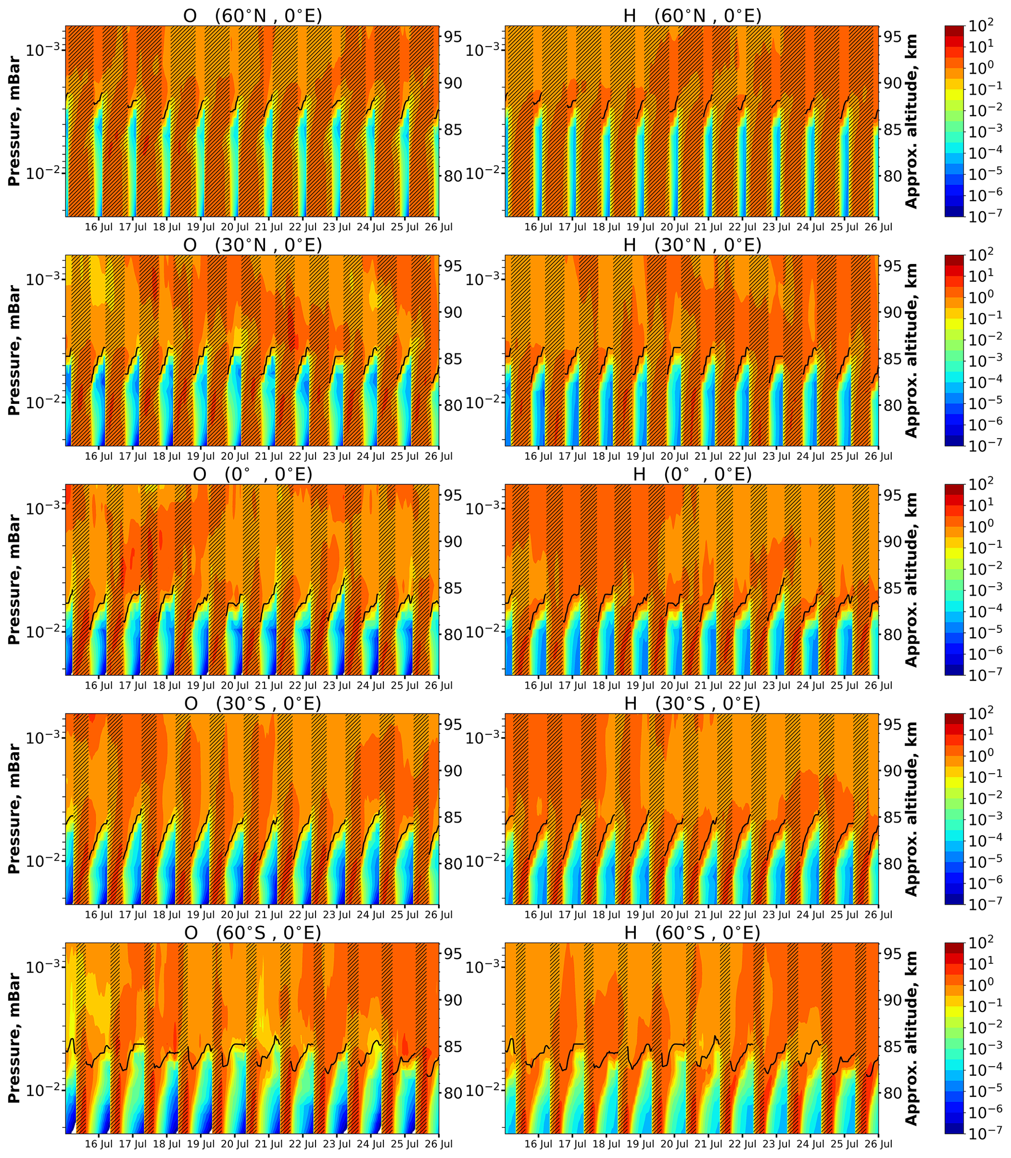
Figure 3 The same as in Fig. 1 but in July 2000. Black lines point the NOCE boundary altitude according to Criterion (5) (Cr=0.1).

Kulikov et al. (2023) presented the theory of chemical equilibrium of a certain trace gas n. Strictly mathematically, the cascade of sufficient conditions for $n_i\left(t\right)\cong n_i^{\mathrm{eq}}\left(t\right)$ was derived considering its lifetime, equilibrium concentration, and time dependences of these characteristics. In case of the nighttime ozone, it was proved that ${\mathit{\tau }}_{{\mathrm{O}}_{\mathrm{3}}}/{\mathit{\tau }}_{{\mathrm{O}}_{\mathrm{3}}^{\mathrm{eq}}}\ll \mathrm{1}$ is the main condition for NOCE validity, and the criterion ${\mathit{\tau }}_{{\mathrm{O}}_{\mathrm{3}}}/{\mathit{\tau }}_{{\mathrm{O}}_{\mathrm{3}}^{\mathrm{eq}}}\le \mathrm{0.1}$ limits a possible difference between O₃ and ${\mathrm{O}}_{\mathrm{3}}^{\mathrm{eq}}$ to not more than ∼ 10 %. Moreover, Kulikov et al. (2023) slightly corrected the expression for Criterion (4):

$$\begin{array}{}\text{(5)}& \begin{array}{rl}\mathrm{Cr}& =\mathrm{2}{\displaystyle \frac{k_{\mathrm{1}}\cdot {\mathrm{O}}_{\mathrm{2}}\cdot \mathrm{M}}{k_{\mathrm{2}}}}(k_{\mathrm{4}}\cdot \mathrm{M}\cdot {\mathrm{O}}_{\mathrm{2}}\cdot \left(\mathrm{1}-{\displaystyle \frac{k_{\mathrm{5}}+k_{\mathrm{6}}}{k_{\mathrm{3}}}}\right)\\ & +k_{\mathrm{2}}\cdot {\mathrm{O}}_{\mathrm{3}})\cdot {\displaystyle \frac{\mathrm{1}}{k_{\mathrm{2}}\cdot \mathrm{H}\cdot {\mathrm{O}}_{\mathrm{3}}}}\le \mathrm{0.1}.\end{array}\end{array}$$

One more important condition for ${\mathrm{O}}_{\mathrm{3}}\approx {\mathrm{O}}_{\mathrm{3}}^{\mathrm{eq}}$ at the time moment t is

$$\begin{array}{}\text{(6)}& e^{{\int }_{t_{\mathrm{bn}}}^t{\mathit{\tau }}_{{\mathrm{O}}_{\mathrm{3}}}^{-\mathrm{1}}\mathrm{d}t}\gg \mathrm{1},\end{array}$$

where t_bn is the time of the beginning of the night. The ozone equilibrium concentration jumps at sunset due to the shutdown of photodissociation. Thus, Condition (6) shows that it takes time for the ozone concentration to reach a new equilibrium. Kulikov et al. (2023) revealed that, at the solar zenith angle χ>95^∘, Condition (6) is fulfilled almost in all cases and Condition (5) becomes the main criterion for NOCE validity. In addition, Kulikov et al. (2023) demonstrated with the use of a 3D model that Criterion (5) almost ideally reproduces the NOCE boundary found by direct comparison of O₃ and ${\mathrm{O}}_{\mathrm{3}}^{\mathrm{eq}}$ concentrations; see Fig. 1 in Kulikov et al. (2023).

Figure 4 Time evolution of monthly-mean pressure altitude $h_{\mathrm{eq}}^{\mathrm{m}}$ at different latitudes.

Figures 1–3 demonstrate model examples of O and H time–height variations above different points over 3 months. In order to focus attention on diurnal oscillations, the concentrations are normalized by mean daily values, which were calculated as a function of altitude. These daily average O and H values were different for each altitude. One can see in all panels of these figures deep diurnal oscillations that occur below 81–87 km. Due to the shutdown of sources at night and high rates of the main HO_x and O sinks nonlinearly dependent on air concentration (Konovalov and Feigin, 2000), the variables change during each night within the range of several orders of magnitude with low values of time evolution. Above 83–88 km, the situation differs essentially from the previous case. One can see relatively weak diurnal oscillations. These regimes of O and H behavior are consistent, i.e., deep H diurnal oscillations correspond to the same dynamics in O, and so on. There exists a few-kilometers-thick layer (transition zone) dividing deep and weak oscillations whose height position depends on latitude and season. In particular, in summer the middle-latitude transition is higher than in winter. Figures 1–3 also show the magenta lines pointing out the NOCE boundary in accordance with Criterion (5) (Cr=0.1). One can see that the NOCE criterion almost perfectly reproduces the features of the transition zone. Thus, our criterion is not only a useful technical characteristic to retrieve O from satellite data, but it also points to an important dynamical process in the O_x-HO_x photochemistry.

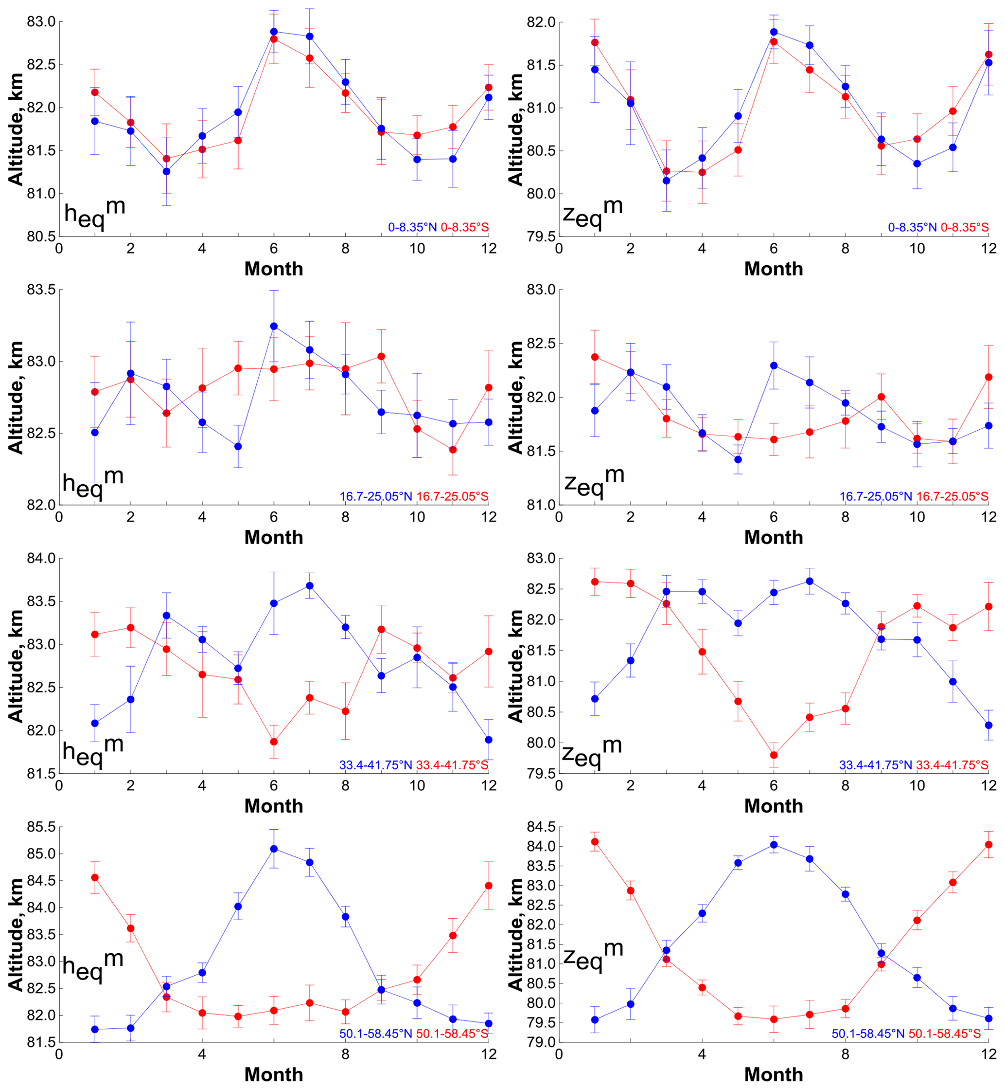
Figure 5 Average (for 2002–2021) annual cycle of monthly-mean pressure altitude $h_{\mathrm{eq}}^{\mathrm{m}}$ and geometrical altitude $z_{\mathrm{eq}}^{\mathrm{m}}$ at four specific latitudes.

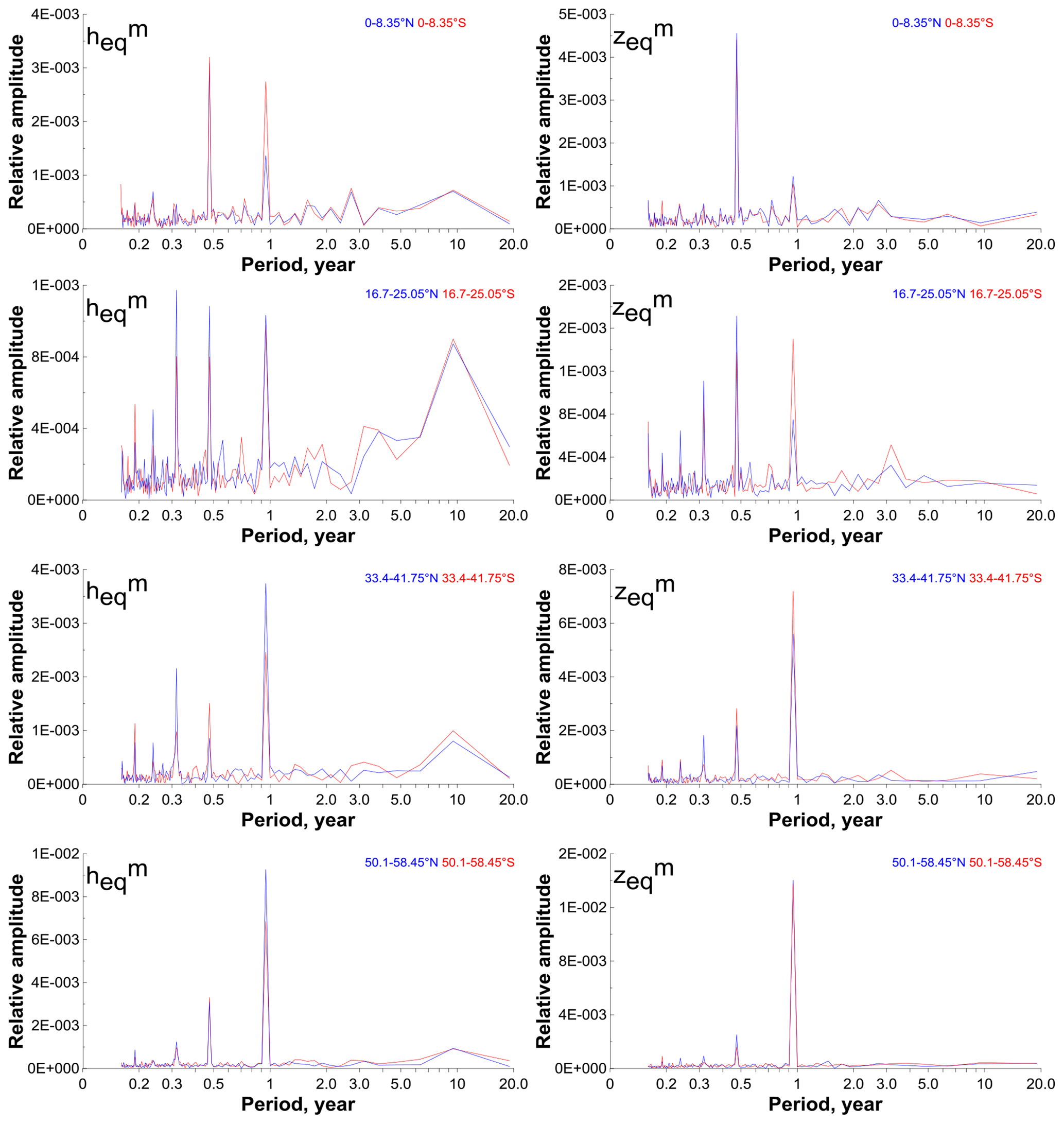
Figure 6 Fourier spectra of monthly-mean pressure altitude $h_{\mathrm{eq}}^{\mathrm{m}}$ and geometrical altitude $z_{\mathrm{eq}}^{\mathrm{m}}$ at four specific latitudes. In each spectrum, the amplitudes of harmonics were normalized to the corresponding zero harmonic.

4 NOCE boundary from satellite data

We use version 2.0 of the SABER data product (level 2A) for the simultaneously measured profiles of pressure (p), altitude (z), temperature (T), O₃ (at 9.6 µm), and total volume emission rates of OH* transitions at 2.0 µm (denoted VER) within the 0.0001–0.02 mbar pressure interval (altitudes approximately 75–105 km) in 2002–2021. We consider only nighttime data when the solar zenith angle χ>95^∘.

Kulikov et al. (2018a) noted that the term $k_{\mathrm{2}}\cdot \mathrm{H}\cdot {\mathrm{O}}_{\mathrm{3}}$ in the expression for the NOCE criterion can be rewritten in the form depending on measurable characteristics only with the use of the corresponding OH(v) model by Mlynczak et al. (2013a):

$$\begin{array}{}\text{(7)}& k_{\mathrm{2}}\cdot \mathrm{H}\cdot {\mathrm{O}}_{\mathrm{3}}=\mathrm{VER}/A(\mathrm{T},\mathrm{M},\mathrm{O}),\end{array}$$

where $A\left(\mathrm{T},\mathrm{M},\mathrm{O}\right)$ is the function in square brackets in Eq. (3) in the paper by Mlynczak et al. (2013a) with the parameters corrected by Mlynczak et al. (2018):

$$\begin{array}{}\text{(8)}& \begin{array}{rl}& A\left(\mathrm{T},\mathrm{M},\mathrm{O}\right)\\ & ={\displaystyle \frac{\mathrm{0.47}\cdot \mathrm{118.35}}{\mathrm{215.05}+\mathrm{2.5}\cdot {\mathrm{10}}^{-\mathrm{11}}\cdot {\mathrm{O}}_{\mathrm{2}}+\mathrm{3.36}\cdot {\mathrm{10}}^{-\mathrm{13}}\cdot e^{\frac{\mathrm{220}}{\mathrm{T}}}\cdot {\mathrm{N}}_{\mathrm{2}}+\mathrm{3}\cdot {\mathrm{10}}^{-\mathrm{10}}\cdot \mathrm{O}}}\\ & +{\displaystyle \frac{\mathrm{0.34}\cdot \mathrm{117.21}}{\mathrm{178.06}+\mathrm{4.8}\cdot {\mathrm{10}}^{-\mathrm{13}}\cdot {\mathrm{O}}_{\mathrm{2}}+\mathrm{7}\cdot {\mathrm{10}}^{-\mathrm{13}}\cdot {\mathrm{N}}_{\mathrm{2}}+\mathrm{1.5}\cdot {\mathrm{10}}^{-\mathrm{10}}\cdot \mathrm{O}}}\\ & +{\displaystyle \frac{\begin{array}{c}\mathrm{0.47}\cdot \mathrm{117.21}\cdot \\ (\mathrm{20.05}+\mathrm{4.2}\cdot {\mathrm{10}}^{-\mathrm{12}}\cdot {\mathrm{O}}_{\mathrm{2}}+\mathrm{4}\cdot {\mathrm{10}}^{-\mathrm{13}}\cdot {\mathrm{N}}_{\mathrm{2}})\end{array}}{\begin{array}{c}(\mathrm{215.05}+\mathrm{2.5}\cdot {\mathrm{10}}^{-\mathrm{11}}\cdot {\mathrm{O}}_{\mathrm{2}}+\mathrm{3.36}\cdot {\mathrm{10}}^{-\mathrm{13}}\cdot e^{\frac{\mathrm{220}}{\mathrm{T}}}\cdot {\mathrm{N}}_{\mathrm{2}}+\mathrm{3}\cdot {\mathrm{10}}^{-\mathrm{10}}\cdot \mathrm{O})\\ \cdot (\mathrm{178.06}+\mathrm{4.8}\cdot {\mathrm{10}}^{-\mathrm{13}}\cdot {\mathrm{O}}_{\mathrm{2}}+\mathrm{7}\cdot {\mathrm{10}}^{-\mathrm{13}}\cdot {\mathrm{N}}_{\mathrm{2}}+\mathrm{1.5}\cdot {\mathrm{10}}^{-\mathrm{10}}\cdot \mathrm{O})\end{array}}}.\end{array}\end{array}$$

This function is the result of the combination of the equations of physicochemical OH* balance in the v=8 and v=9 states. It depends on the constants of the processes describing sources and sinks at the corresponding levels, in particular the OH(v) removal on collisions with O₂, N₂, and O. Below 86–87 km, $A(\mathrm{T},\mathrm{M},\mathrm{O})\cong A(\mathrm{T},\mathrm{M},\mathrm{O}=\mathrm{0})\equiv A(\mathrm{T},\mathrm{M})$ due to relatively small O concentrations. Thus, by combining Eqs. (5) and (7), the NOCE criterion for SABER data can be recast in the following form:

$$\begin{array}{}\text{(9)}& \begin{array}{rl}& \mathrm{VER}\ge {\mathrm{VER}}_{\min }\left(\mathrm{T},\mathrm{M}\right)=\mathrm{20}\cdot {\displaystyle \frac{k_{\mathrm{1}}\cdot {\mathrm{O}}_{\mathrm{2}}\cdot \mathrm{M}}{k_{\mathrm{2}}}}\\ & \left(k_{\mathrm{4}}\cdot {\mathrm{O}}_{\mathrm{2}}\cdot \mathrm{M}\cdot \left(\mathrm{1}-{\displaystyle \frac{k_{\mathrm{5}}+k_{\mathrm{6}}}{k_{\mathrm{3}}}}\right)+k_{\mathrm{2}}\cdot {\mathrm{O}}_{\mathrm{3}}\right)\cdot A(\mathrm{T},\mathrm{M}).\end{array}\end{array}$$

Due to the strong air-concentration dependence, VER_min decreases rapidly with height. In particular, at 105 km, VER ≫VER_min. At 75 km, the relationship is inverse. We determine the local position of the NOCE boundary (pressure level $p_{\mathrm{eq}}^{\mathrm{l}}$ and altitude level $z_{\mathrm{eq}}^{\mathrm{l}}$) according to Criterion (9), where $\mathrm{VER}={\mathrm{VER}}_{\min }\left(\mathrm{T},\mathrm{M}\right)$. We verified that the approximation $A(\mathrm{T},\mathrm{M},\mathrm{O})\cong A(\mathrm{T},\mathrm{M})$ is valid near the NOCE boundary. With the use of annual SABER data, we calculated simultaneous datasets of A(T,M) and $A\left(\mathrm{T},\mathrm{M},\mathrm{O}\right)$. In the second case, we used O retrieved from the same SABER data. The maximum and mean differences between A(T,M) and $A\left(\mathrm{T},\mathrm{M},\mathrm{O}\right)$ were found to be ∼ 2 % and ∼ 0.1 %, respectively.

The total range of latitudes according to the satellite trajectory over a month was ∼ 83.5^∘ S–83.5^∘ N. This range was divided into 20 bins, and all local values of $p_{\mathrm{eq}}^{\mathrm{l}}$ and $z_{\mathrm{eq}}^{\mathrm{l}}$ falling into one bin during a month or a year were averaged, respectively. In particular, several thousand values of $p_{\mathrm{eq}}^{\mathrm{l}}$ and $z_{\mathrm{eq}}^{\mathrm{l}}$ fall into one bin during a month. Following Mlynczak et al. (2013a), averages were determined by binning the data of a certain day by local hour and then averaging over the hour bins that contain data to obtain the daily average value. Then we calculated monthly-mean values of $p_{\mathrm{eq}}^{\mathrm{m}}$ and $z_{\mathrm{eq}}^{\mathrm{m}}$ and annually mean values of $p_{\mathrm{eq}}^{\mathrm{y}}$ and $z_{\mathrm{eq}}^{\mathrm{y}}$ (hereafter, the indexes “m” and “y” indicate the monthly and annually averages, respectively). Then, for convenience, the values of $p_{\mathrm{eq}}^{\mathrm{m}}$ and $p_{\mathrm{eq}}^{\mathrm{y}}$ were recalculated to the pressure altitudes $h_{\mathrm{eq}}^{\mathrm{m}}$ and $h_{\mathrm{eq}}^{\mathrm{y}}$. The dependence of $h_{\mathrm{eq}}^{\mathrm{m},\mathrm{y}}$ on $p_{\mathrm{eq}}^{\mathrm{m},\mathrm{y}}$ was adopted from Mlynczak et al. (2013a, 2014):

$$\begin{array}{}\text{(10)}& \begin{array}{rl}& h_{\mathrm{eq}}^{\mathrm{m},\mathrm{y}}=-H_{\mathrm{a}}\cdot \log (p_{\mathrm{eq}}^{\mathrm{m},\mathrm{y}}/p_{\mathrm{0}}),H_{\mathrm{a}}=\mathrm{5.753474},\\ & p_{\mathrm{0}}=\mathrm{11430.49428}\mathrm{hPa}.\end{array}\end{array}$$

Note that the use of both geometrical and pressure coordinates is a rather common approach when analyzing long-term evolution of the obtained data, especially when the data are the result of averaging over time and space. In particular, Lübken et al. (2013) demonstrated the importance of distinguishing between trends on pressure and geometrical altitudes in the mesosphere, since the second includes the atmospheric shrinking effect and is more pronounced. Grygalashvyly et al. (2014) analyzed the linear trends in OH^∗ peak height and revealed a remarkable decrease at geometrical altitudes, which is almost absent at pressure altitudes.

Kulikov et al. (2023) studied the systematic uncertainty of the retrieved NOCE boundary height. Following the typical analysis presented, for example, in Mlynczak et al. (2013a, 2014), the uncertainty was obtained by calculating the root sum square of the individual sensitivity of the retrieved characteristic to the perturbation of O₃, T, rates of reactions, and parameters of the A function. The systematic error of NOCE pressure altitude $h_{\mathrm{eq}}^{\mathrm{m}}$ and geometrical altitude $z_{\mathrm{eq}}^{\mathrm{m}}$ varied in the range 0.1–0.3 km, whereas the random error was negligible due to averaging over time and space.

5 NOCE boundary in 2002–2021 from SABER/TIMED data: main results

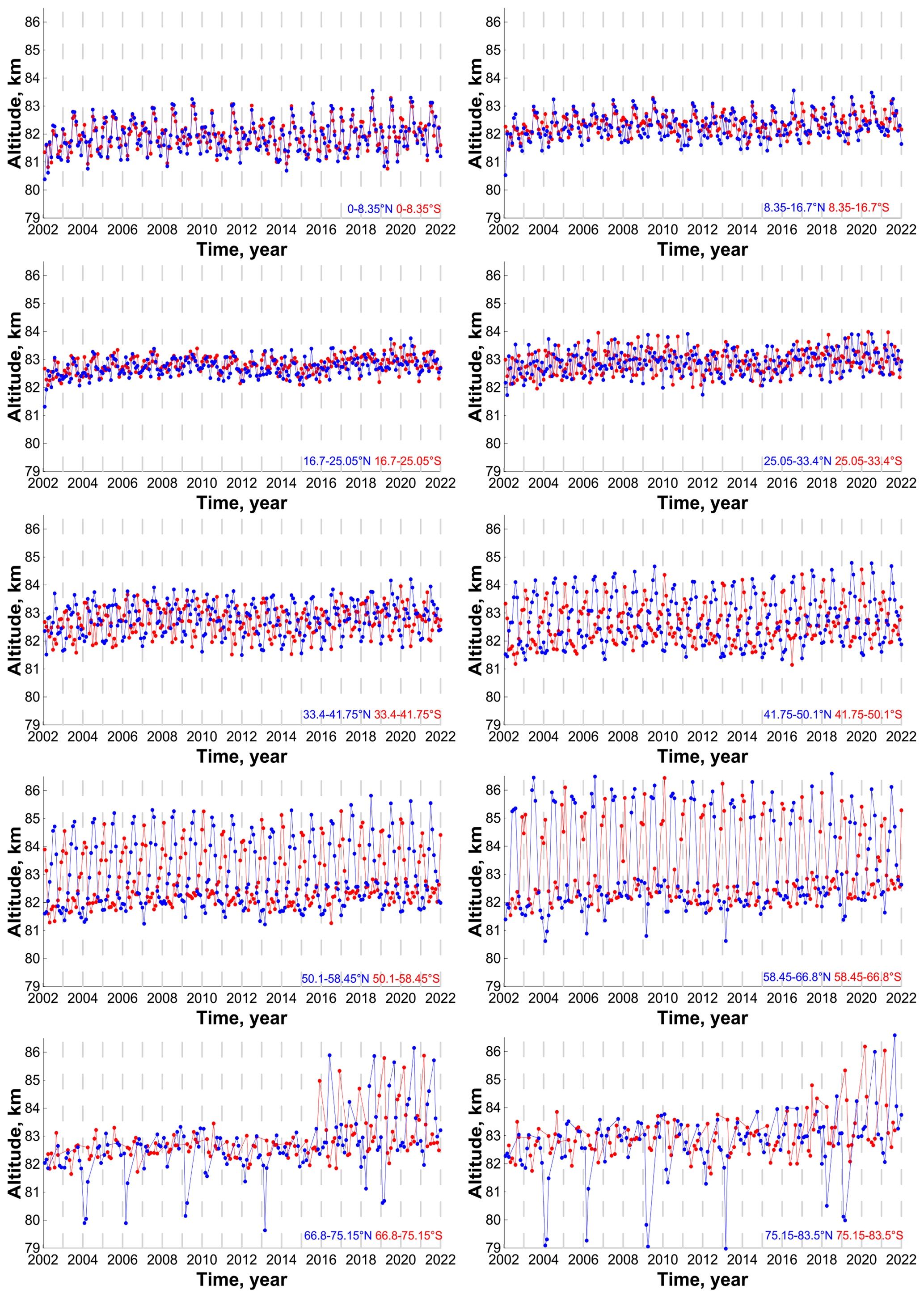
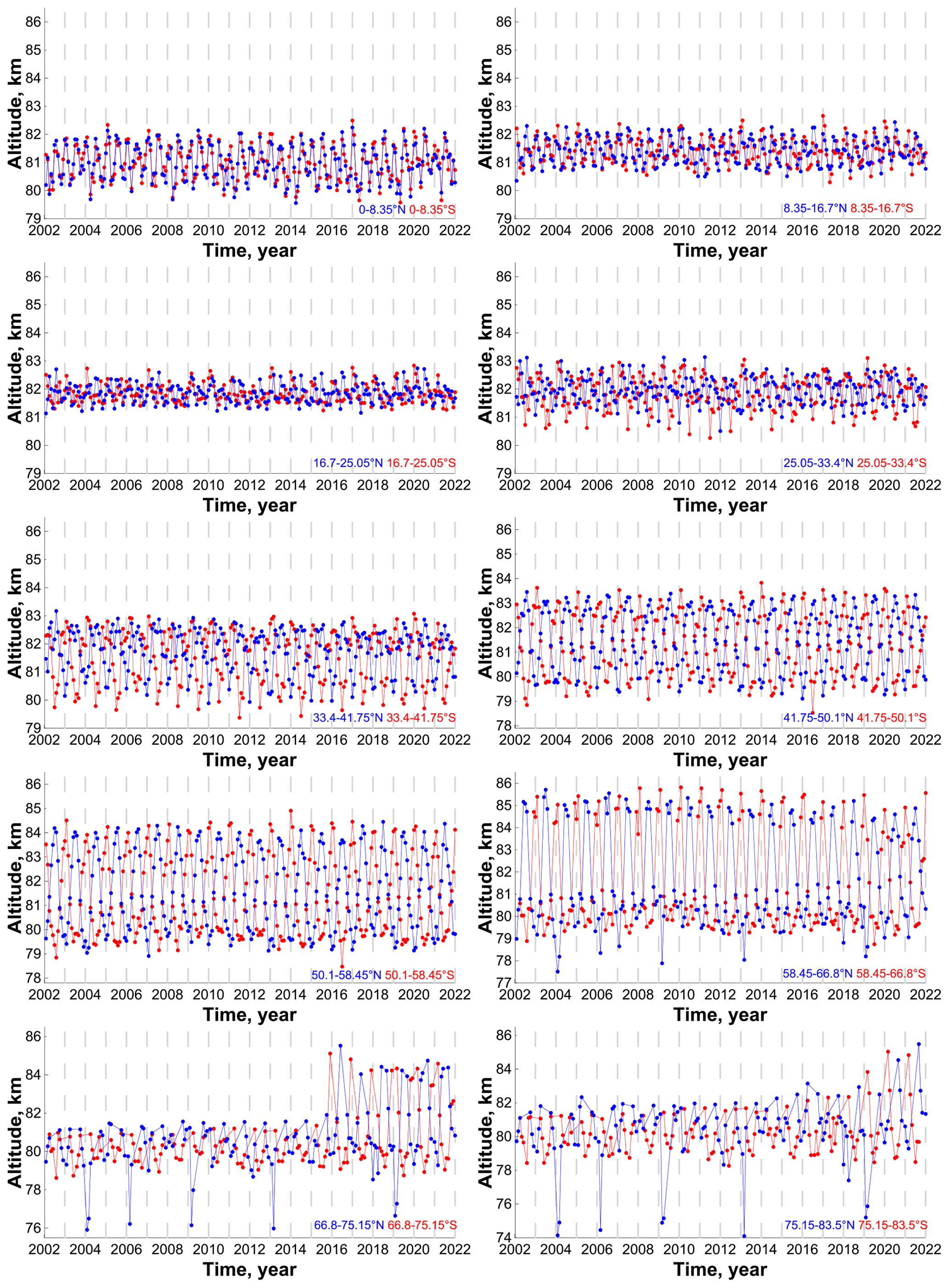
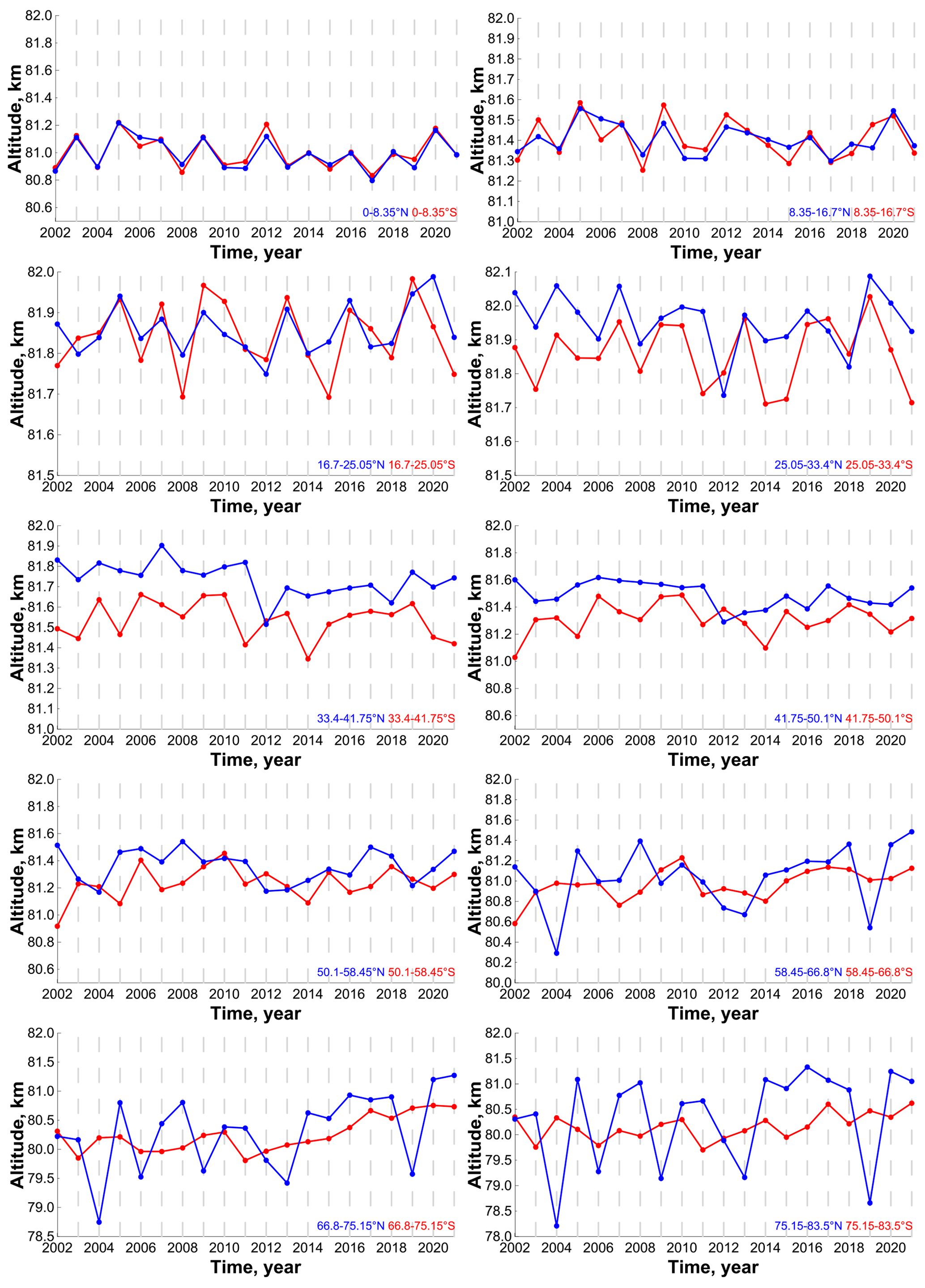
Figure 4 demonstrates the time evolution of the pressure altitude $h_{\mathrm{eq}}^{\mathrm{m}}$ in 2002–2021 in all latitude bins. Figure 5 (left column) shows the mean (for 2002–2021) annual cycle of $h_{\mathrm{eq}}^{\mathrm{m}}$ at four specific latitudes, and Fig. 6 (left column) presents the Fourier spectra at these latitudes obtained from the data in Fig. 4. Note, first, that above ∼ 58^∘ S and N, there are data gaps specified by the satellite sensing geometry. For example, in 2002–2014, at 66.8–75.15^∘ S and N measurements covered 6 months per year only. In 2015, because of slight changes in the satellite geometry, there appeared additional months. This is especially noticeable above ∼ 66^∘ S and N and manifests itself by extension of the variation range of $h_{\mathrm{eq}}^{\mathrm{m}}$ at these latitudes in 2015–2021. Second, the variation range of $h_{\mathrm{eq}}^{\mathrm{m}}$, annual cycle and spectrum of harmonic oscillations, depends essentially on the latitude. Near the Equator, $h_{\mathrm{eq}}^{\mathrm{m}}$ varies in the 81–83 km range mainly, and there are two main harmonics with periods of 1/2 and 1 year in the spectrum. At low latitudes, the variation range of $h_{\mathrm{eq}}^{\mathrm{m}}$ narrows down to a minimum (∼ 82–83 km at 16.7–20.05^∘S, N), which is accompanied with the appearance of a wide spectrum of harmonics with periods of 1/5, 1/4, 1/3, 1/2, and 1 year. At middle latitudes, the range of $h_{\mathrm{eq}}^{\mathrm{m}}$ variation monotonically increases up to ∼ 81.5–85.5 km with latitude and the harmonic with a period of 1 year becomes the main mode in the spectrum of oscillations. At both low and middle latitudes, there is no signal from quasi-biennial oscillations but one can see a remarkable amplitude of a harmonic with a period of ∼ 10 years, which can be associated with a manifestation of an 11-year solar cycle. It is interesting that the mentioned features are typical for both hemispheres. At high latitudes, $h_{\mathrm{eq}}^{\mathrm{m}}$ varies in the range 79–86.5 km. At these latitudes, one can see the main difference between the Northern Hemisphere and Southern Hemisphere: the sharp falls and rises of the northern boundary of NOCE by several kilometers (up to 3–4 km) appearing in January–March 2004, 2006, 2009, 2010, 2012, 2013, 2018 and 2019 that are absent at southern latitudes.

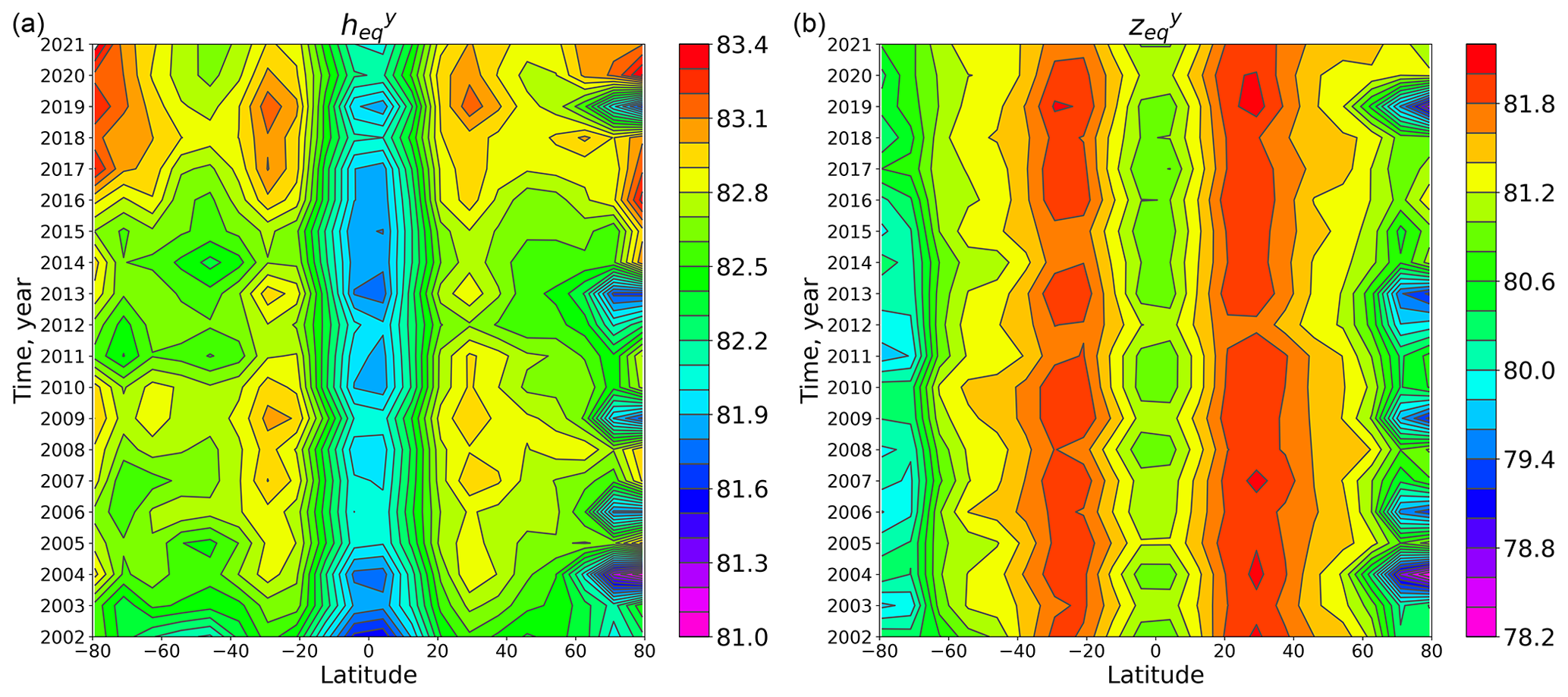
Figure 7 Latitude–time evolution of annually mean pressure altitude $h_{\mathrm{eq}}^{\mathrm{y}}$ (a) and geometrical altitude $z_{\mathrm{eq}}^{\mathrm{y}}$ (b).

Figure 8 Time evolution of annually mean pressure altitude $h_{\mathrm{eq}}^{\mathrm{y}}$ at different latitudes.

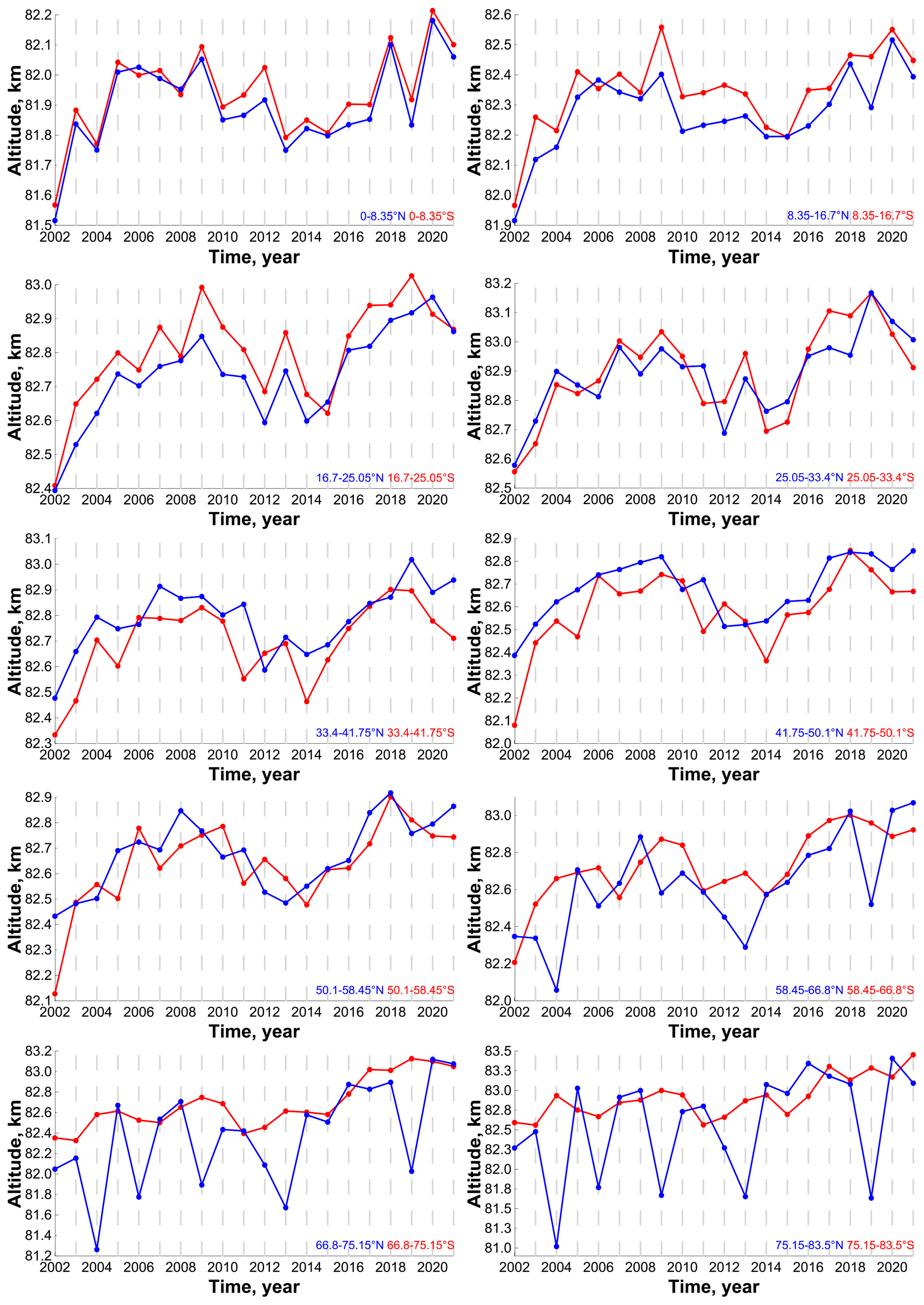
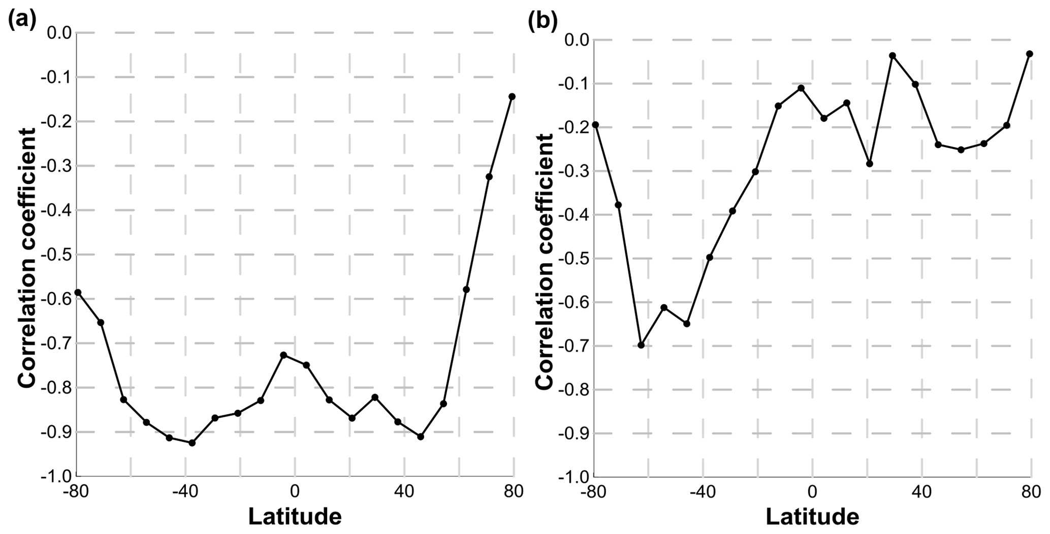
Figure 9 Correlation coefficient of the F_10.7 index with pressure altitude $h_{\mathrm{eq}}^{\mathrm{y}}$ (a) and geometrical altitude $z_{\mathrm{eq}}^{\mathrm{y}}$ (b) as a function of latitude.

The analysis of Figs. 5–6 demonstrates the following redistribution in the annual cycle with increasing latitude from Equator to polar latitudes. Near the Equator, the annual cycle has two maxima in June–July and in December–January. The first one is more pronounced. That is why there are two main harmonics with periods of 1/2 and 1 year in the spectrum. At low latitudes, one maximum (summer) does not change, while the other approaches the first one. As a result, the spectrum of harmonics is wide. At middle latitudes, the maxima gradually merge so that the 1-year harmonic becomes the main one.

Figure 7 (left) demonstrates a contour map of the space–time evolution of the average annual pressure altitude $h_{\mathrm{eq}}^{\mathrm{y}}$ in 2002–2021. Figure 8 presents the time evolution of this characteristic at different latitudes. Based on the Fourier spectra presented in Fig. 6 (left column), we can suppose that, at low and middle latitudes, the interannual variation of $h_{\mathrm{eq}}^{\mathrm{y}}$ is caused by the 11-year solar cycle mainly. Figure 9 (left) presents the correlation coefficient of $h_{\mathrm{eq}}^{\mathrm{y}}$ with the F_10.7 index (solar radio flux at 10.7 cm; see the red curve in Fig. 10) as a function of latitude. One can see good anticorrelation (with a coefficient from −0.72 to −0.92) between ∼ 55^∘ S and ∼ 55^∘ N. At high latitudes, the absolute value of the correlation coefficient decreases sharply down to ∼ 0.58 in the south and to ∼ 0.1 in the north. The blue curve in Fig. 10 shows latitude-averaged $h_{\mathrm{eq}}^{\mathrm{y}}$ in the range 55^∘ S–55^∘ N. In this case, the anticorrelation with the F_10.7 index is close to ideal (coefficient ∼ −0.95).

With the use of multiple linear regression in the 55^∘ S–55^∘ N range,

$$\begin{array}{}\text{(11)}& h_{\mathrm{eq}}^{\mathrm{y}}\left(\mathrm{year}\right)=\mathrm{const}+\mathit{\alpha }\cdot \mathrm{year}+\mathit{\beta }\cdot F_{\mathrm{10.7}}\left(\mathrm{year}\right),\end{array}$$

we determined a slow (up to 10 m yr⁻¹) linear trend of $h_{\mathrm{eq}}^{\mathrm{y}}$ as a function of latitude but with the uncertainties essentially larger than the trend values. Applying the regression analysis to latitude-averaged $h_{\mathrm{eq}}^{\mathrm{y}}$ (blue curve in Fig. 10) gave us a more statistically significant value of the trend: 5.62±4.22 m yr⁻¹.

Figure 11 demonstrates the time evolution of the geometrical altitude $z_{\mathrm{eq}}^{\mathrm{m}}$ in 2002–2021 in all latitude bins. Figures 5 (right column) shows the mean (for 2002–2021) annual cycle of $z_{\mathrm{eq}}^{\mathrm{m}}$ at four specific latitudes and Fig. 6 (right column) presents the Fourier spectra at these latitudes obtained from the data in Fig. 11. Comparison with Figs. 4 and 5–6 (left columns) shows that $z_{\mathrm{eq}}^{\mathrm{m}}$ repeats many qualitative features of the space–time evolution of pressure altitude $h_{\mathrm{eq}}^{\mathrm{m}}$. In particular, in the direction from the Equator to the poles, the variation range of $z_{\mathrm{eq}}^{\mathrm{m}}$ first decreases down to 1 km at 16^∘–25^∘ S and N and then expands to several kilometers at middle and high latitudes. One can see the same redistribution of the annual cycle with latitude, similarly to the pressure altitude case. Near the Equator, the annual cycle possesses two maxima occurring in June–July and in December–January. At low latitudes, one maximum continues in summer, whereas the other shifts to spring. At middle latitudes, the maxima gradually coalesce forming a single summer maximum. At high northern latitudes, there are the same local sharp variations of the NOCE boundary in January–February 2004, 2006, 2009, 2010, 2012, 2013, 2018 and 2019, which are absent at southern latitudes. One can see from Fig. 5 that, on the average, $z_{\mathrm{eq}}^{\mathrm{m}}$ is lower than $h_{\mathrm{eq}}^{\mathrm{m}}$ by 0.5–1 km, depending on latitude. One can see from Fig. 6 that the $z_{\mathrm{eq}}^{\mathrm{m}}$ spectra of harmonic oscillations are similar to the $h_{\mathrm{eq}}^{\mathrm{m}}$ spectra except for the absence of a signal of the 11-year solar cycle.

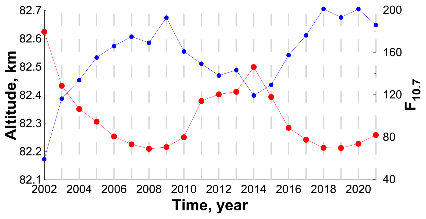
Figure 10 Red curve: the F_10.7 index (solar radio flux at 10.7 cm). Blue curve: latitude-averaged pressure altitude $h_{\mathrm{eq}}^{\mathrm{y}}$ in the range between ∼ 55^∘ S and ∼ 55^∘ N.

Figure 7 (right) demonstrates a contour map of space–time evolution of the annually average geometrical altitude $z_{\mathrm{eq}}^{\mathrm{y}}$ in 2002–2021. Figure 12 presents the time evolution of this characteristic at different latitudes. One can see that there is no clear evidence of an 11-year solar cycle manifestation at all latitudes. This is confirmed by the calculation of the correlation coefficient of $z_{\mathrm{eq}}^{\mathrm{y}}$ with the F_10.7 index as a function of latitude (see Fig. 9 (right)). Moreover, the latitude-averaged (in the range 55^∘ S–55^∘ N) $z_{\mathrm{eq}}^{\mathrm{y}}$ has a correlation coefficient equal to ∼ −0.55.

As in the case of $h_{\mathrm{eq}}^{\mathrm{y}}$, we found with the use of multiple linear regression the slow (up to ∼ −10 m yr⁻¹) and statistically insignificant linear trend of $z_{\mathrm{eq}}^{\mathrm{y}}$ as a function of latitude. Moreover, the regression analysis of latitude-averaged $z_{\mathrm{eq}}^{\mathrm{y}}$ also revealed a statistically insignificant trend.

Figure 11 Time evolution of monthly-mean geometrical altitude $z_{\mathrm{eq}}^{\mathrm{m}}$ at different latitudes.

Figure 12 Time evolution of annually mean geometrical altitude $z_{\mathrm{eq}}^{\mathrm{y}}$ at different latitudes.

6 Discussion

The NOCE boundary is an important technical characteristic for correct application of the NOCE approximation to retrieve the nighttime distributions of minor chemical species of MLT. Kulikov et al. (2019) repeated the O and H retrieval by Mlynczak et al. (2018) from the SABER data for the year 2004. It was revealed that the application of the NOCE condition below the boundary obtained according to the criterion could lead to a great (up to 5–8 times) systematic underestimation of O concentration below 86 km, whereas it was insignificant for H retrieval. The results presented in Figs. 4, 5, and 11 demonstrate that, except for high northern latitudes, there is a stable annual cycle of the NOCE boundary. The monthly-mean boundary can rise up to geometrical altitudes of 82–83 km (∼ (5.2–6.2) × 10⁻³ hPa) at low latitudes and up to 84–85 km (∼ (3.7–4.4) × 10⁻³ hPa) at middle and high latitudes. Thus, the SABER O data below these altitudes/pressures may be essentially incorrect, and the retrieval approaches without using the NOCE condition (e.g., Panka et al., 2018) should be more appropriate.

Note that the NOCE condition was not just used for O and H derivation from satellite data. This assumption is a useful approach helping to (i) study hydroxyl emission in the MLT region with simulated and measured data, in particular OH* mechanisms, morphology, and variability caused, for example, by atmospheric tides and gravity wave activity (e.g., Marsh et al., 2006; Nikoukar et al., 2007; Xu et al., 2010, 2012; Kowalewski et al., 2014; Sonnemann et al., 2015); (ii) analyze the MLT response to sudden stratospheric warmings (SSWs) (e.g., Smith et al., 2009); (iii) derive exothermic heating rates of MLT (e.g., Mlynczak et al., 2013b); (iv) analytically simulate the mesospheric OH* layer response to gravity waves (e.g., Swenson and Gardner, 1998); and (v) derive the analytical dependence of excited hydroxyl layer number density and peak altitude on atomic oxygen and temperature (e.g., Grygalashvyly et al., 2014; Grygalashvyly, 2015). Perhaps some results require revision or reanalysis taking the NOCE boundary into account. For example, Smith et al. (2009) used the NOCE condition to analyze the ozone perturbation in the MLT, in particular during the SSW at the beginning of 2009 (the central day was 24 January). Our preliminary results of processing the SABER and simulated data in January 2009 show that the NOCE boundary above 70^∘ N may jump from ∼ 80 km to ∼ 90–95 km due to a short-time abrupt temperature fall above 80 km during this SSW. Thus, one can assume that the NOCE condition is not a good approximation for the description of ozone variations directly in the process of SSWs. This case will be studied in a separate work. Note also that after the SSW of January 2009 there began a long-time (several tens of days) event of elevated (up to ∼ 80–85 km) stratopause (see, e.g., Fig. 1 in Smith et al., 2009), which led to the corresponding increase of temperature above 80 km. The occurrence of this event and its duration are in a good correlation with a sharp lowering of the NOCE boundary at high northern latitudes (see Figs. 4 and 11). Moreover, all abrupt changes of the NOCE boundary at these latitudes in January–March of other years (2004, 2006, 2010, 2012, 2013, 2018, and 2019) can be also associated with the elevated stratopause events in these years (see García-Comas et al. (2020) and references therein).

According to the used chemical transport model, the NOCE boundary reproduces well the transition zone dividing deep and weak diurnal oscillations of O and H (see Figs. 1–3). We verified this feature with the annual run of the SD-WACCM-X model for the year 2017 provided by the National Center for Atmospheric Research (NCAR) High Altitude Observatory (https://doi.org/10.26024/5b58-nc53). Despite the low time resolution of the downloaded data (3 h averaging), we obtained results (see Fig. 13) similar to Figs. 1–3. Note also that both models give the same consistence between the altitudes of the NOCE boundary and the mentioned transition zone at high latitudes in spring and autumn.

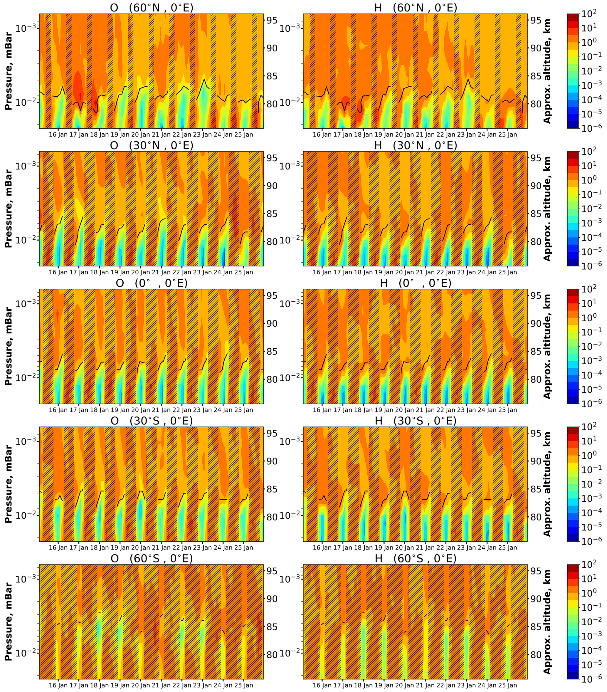
Figure 13 O and H time–height variations above different points in January 2017 calculated by SD-WACCM-X model. Concentrations are normalized by mean daily values, correspondingly. Dark bars mark daytime; light bars mark nighttime. Black lines point out the NOCE boundary altitude according to Criterion (5) (Cr=0.1).

The space–time evolution of the NOCE boundary expressed in terms of pressure altitudes contains a clear signal of the 11-year solar cycle in the 55^∘ S–55^∘ N range, which is suppressed mainly at high latitudes. The weak correlation of $h_{\mathrm{eq}}^{\mathrm{y}}$ with the F_10.7 index at high southern latitudes may be caused by the mentioned data gaps specified by the satellite sensing geometry. The same reason and distortions by SSWs evidently determine no correlation at high northern latitudes. Thus, at low and middle latitudes $h_{\mathrm{eq}}^{\mathrm{y}}$ can be considered as a sensitive indicator of solar activity. Below, we present a simple and short explanation for this. Let us consider the NOCE Criterion (9) at the pressure level p_eq:

$$\mathrm{VER}\left(p_{\mathrm{eq}}\right)={\mathrm{VER}}_{\min }\left(\mathrm{T},\mathrm{M}\left(p_{\mathrm{eq}}\right)\right)$$

In a zero approximation

$$\begin{array}{rl}& {\mathrm{VER}}_{\min }=\mathrm{20}\\ & \cdot {\displaystyle \frac{\begin{array}{c}{k}_{\mathrm{1}}\cdot {\mathrm{O}}_{\mathrm{2}}\left(p_{\mathrm{eq}}\right)\cdot \mathrm{M}\left(p_{\mathrm{eq}}\right)\cdot \left(k_{\mathrm{4}}\cdot {\mathrm{O}}_{\mathrm{2}}\left(p_{\mathrm{eq}}\right)\cdot \mathrm{M}\left(p_{\mathrm{eq}}\right)\right.\\ \cdot \left.\left(\mathrm{1}-\frac{k_{\mathrm{5}}+k_{\mathrm{6}}}{k_{\mathrm{3}}}\right)+k_{\mathrm{2}}\cdot {\mathrm{O}}_{\mathrm{3}}\left(p_{\mathrm{eq}}\right)\right)\cdot A\left(\mathrm{T},\mathrm{M}\left(p_{\mathrm{eq}}\right)\right)\end{array}}{k_{\mathrm{2}}}}\\ & \cong \mathrm{20}\cdot {\displaystyle \frac{k_{\mathrm{1}}\cdot k_{\mathrm{4}}\cdot ({\mathrm{O}}_{\mathrm{2}}\left(p_{\mathrm{eq}}\right)\cdot \mathrm{M}\left(p_{\mathrm{eq}}\right){)}^{\mathrm{2}}\cdot A\left(\mathrm{T},\mathrm{M}\left(p_{\mathrm{eq}}\right)\right)}{k_{\mathrm{2}}}}\\ & \sim {\displaystyle \frac{k_{\mathrm{1}}\cdot k_{\mathrm{4}}\cdot (p_{\mathrm{eq}}/\mathrm{T}{)}^{\mathrm{4}}\cdot A\left(\mathrm{T},p_{\mathrm{eq}}\right)}{k_{\mathrm{2}}}}\\ & \sim {\displaystyle \frac{\exp \left(\mathrm{470}/\mathrm{T}\right)\cdot p_{\mathrm{eq}}^{\mathrm{4}}\cdot A\left(\mathrm{T},p_{\mathrm{eq}}\right)}{{\mathrm{T}}^{\mathrm{8.2}}}},\end{array}$$

where A(T,p_eq)
$=\frac{\mathrm{0.47}\cdot \mathrm{118.35}}{\mathrm{215.05}+\mathrm{2.5}\cdot {\mathrm{10}}^{-\mathrm{11}}\cdot {\mathrm{O}}_{\mathrm{2}}/\mathrm{M}\cdot \frac{p_{\mathrm{eq}}}{k_B\mathrm{T}}+\mathrm{3.36}\cdot {\mathrm{10}}^{-\mathrm{13}}\cdot e^{\frac{\mathrm{220}}{\mathrm{T}}}\cdot {\mathrm{N}}_{\mathrm{2}}/\mathrm{M}\cdot \frac{p_{\mathrm{eq}}}{k_B\mathrm{T}}}$
+ $\frac{\mathrm{0.34}\cdot \mathrm{117.21}}{\mathrm{178.06}+\mathrm{4.8}\cdot {\mathrm{10}}^{-\mathrm{13}}\cdot {\mathrm{O}}_{\mathrm{2}}/\mathrm{M}\cdot \frac{p_{\mathrm{eq}}}{k_B\mathrm{T}}+\mathrm{7}\cdot {\mathrm{10}}^{-\mathrm{13}}\cdot {\mathrm{N}}_{\mathrm{2}}/\mathrm{M}\cdot \frac{p_{\mathrm{eq}}}{k_B\mathrm{T}}}$ + $\frac{\begin{array}{c}\mathrm{0.47}\cdot \mathrm{117.21}\cdot \left(\mathrm{20.05}+\mathrm{4.2}\cdot {\mathrm{10}}^{-\mathrm{12}}\cdot {\mathrm{O}}_{\mathrm{2}}/\mathrm{M}\cdot \frac{p_{\mathrm{eq}}}{k_B\mathrm{T}}\right.\\ \left.+\mathrm{4}\cdot {\mathrm{10}}^{-\mathrm{13}}\cdot {\mathrm{N}}_{\mathrm{2}}/\mathrm{M}\cdot \frac{p_{\mathrm{eq}}}{k_B\mathrm{T}}\right)\end{array}}{\begin{array}{c}(\mathrm{215.05}+\mathrm{2.5}\cdot {\mathrm{10}}^{-\mathrm{11}}\cdot {\mathrm{O}}_{\mathrm{2}}/\mathrm{M}\cdot \frac{p_{\mathrm{eq}}}{k_B\mathrm{T}}+\mathrm{3.36}\cdot {\mathrm{10}}^{-\mathrm{13}}\cdot e^{\frac{\mathrm{220}}{\mathrm{T}}}\cdot {\mathrm{N}}_{\mathrm{2}}/\mathrm{M}\cdot \frac{p_{\mathrm{eq}}}{k_B\mathrm{T}})\\ \cdot (\mathrm{178.06}+\mathrm{4.8}\cdot {\mathrm{10}}^{-\mathrm{13}}\cdot {\mathrm{O}}_{\mathrm{2}}/\mathrm{M}\cdot \frac{p_{\mathrm{eq}}}{k_B\mathrm{T}}+\mathrm{7}\cdot {\mathrm{10}}^{-\mathrm{13}}\cdot {\mathrm{N}}_{\mathrm{2}}/\mathrm{M}\cdot \frac{p_{\mathrm{eq}}}{k_B\mathrm{T}})\end{array}}$.

Our analysis of A(T,p_eq) shows that this function can be approximately rewritten as $A\left(\mathrm{T},p_{\mathrm{eq}}\right)\approx \text{const}+\frac{\text{const}}{\text{const}+\frac{p_{\mathrm{eq}}}{T}}$. So, one can see that VER_min is strongly dependent on T. Moreover, it anticorrelates with T. Gan et al. (2017) and Zhao et al. (2021) analyzed the simulated and measured data and revealed a clear correlation between the MLT temperature above 80 km and the 10.7 cm solar radio flux. Moreover, the dependence of the correlation coefficient of T with the F_10.7 index on latitude in the 55^∘ S–55^∘ N range given in Fig. 9 in the paper by of Zhao et al. (2021) is consistent with our Fig. 9 (left panel), taking into account the sign of the correlation. Thus, we can conclude that the found anticorrelation of the NOCE boundary $h_{\mathrm{eq}}^{\mathrm{y}}$ with solar activity is caused by the strong connection with temperature, which, in turn, is in a good correlation with the F_10.7 index. A detailed analysis of the reasons why the solar cycle weakly manifests itself in the spatiotemporal variability of $z_{\mathrm{eq}}^{\mathrm{y}}$ is not so simple and is beyond the scope of this work.

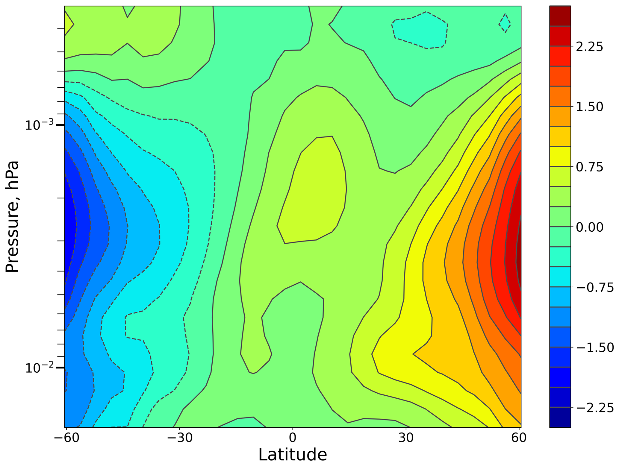
Figure 14 Logarithm of the ratio of (O/H)_w and (O/H)_s distributions obtained with the use of daytime seasonally mean distributions of O and H averaged in 2003–2015. (O/H)_w was determined from the SABER data measured in December, January, and February. (O/H)_s was determined from the SABER data measured in June, July, and August.

Figure 5 illustrates an interesting peculiarity. At middle latitudes, the summer $h_{\mathrm{eq}}^{\mathrm{m}}$ and $z_{\mathrm{eq}}^{\mathrm{m}}$ values are remarkably (by several kilometers) higher than the winter ones, while the opposite relationship could be expected. Due to more effective daytime HO_x photoproduction at these altitudes, the summer H values at the beginning of the night are higher than the ones in winter. So, the summer ozone lifetimes should be shorter and the NOCE condition is more favorable than in winter. Nevertheless, the same ratio between the summer and winter NOCE boundaries at middle latitudes was revealed in Belikovich et al. (2018) and Kulikov et al. (2018a), where the boundary of this equilibrium was determined by direct comparison of O₃ and O${}_{\mathrm{3}}^{\mathrm{eq}}$ concentrations from results of 3D chemical transport models. Based on the results of Sect. 3, we can assume that the discussed effect is connected with the height position of the transition zone, which demonstrates the same variation (see Figs. 1–3). Kulikov et al. (2023) derived the equations describing pure chemical O and H nighttime evolution:

$$\begin{array}{}\text{(12)}& \left\{\begin{array}{l}\frac{\mathrm{dO}}{\mathrm{d}t}=-\mathrm{2}\cdot k_{\mathrm{4}}\cdot \mathrm{M}\cdot {\mathrm{O}}_{\mathrm{2}}\cdot \mathrm{H}-\mathrm{2}\cdot k_{\mathrm{2}}\cdot \mathrm{H}\cdot {\mathrm{O}}_{\mathrm{3}},\\ \frac{\mathrm{dH}}{\mathrm{d}t}=-\mathrm{2}\cdot k_{\mathrm{4}}\cdot \mathrm{M}\cdot {\mathrm{O}}_{\mathrm{2}}\cdot \frac{k_{\mathrm{5}}+k_{\mathrm{6}}}{k_{\mathrm{3}}}\cdot \frac{{\mathrm{H}}^{\mathrm{2}}}{\mathrm{O}}.\end{array}\right.\end{array}$$

Neglecting the second term in the first equation as a secondary one, this system can be solved analytically, so the nighttime evolution times of O and H are

$$\begin{array}{}\text{(13)}& \begin{array}{rl}{\mathit{\tau }}_{\mathrm{O}}& \equiv {\displaystyle \frac{\mathrm{O}}{\left|\mathrm{dO}/\mathrm{d}t\right|}}={\displaystyle \frac{\mathrm{1}}{\mathrm{2}\cdot k_{\mathrm{4}}\cdot \mathrm{M}\cdot {\mathrm{O}}_{\mathrm{2}}}}\cdot {\left({\displaystyle \frac{\mathrm{O}}{\mathrm{H}}}\right)}_{t=t_{\mathrm{bn}}}\\ & -\left(\mathrm{1}-{\displaystyle \frac{k_{\mathrm{5}}+k_{\mathrm{6}}}{k_{\mathrm{3}}}}\right)\cdot (t-t_{\mathrm{bn}}),\end{array}\end{array}$$

$$\begin{array}{}\text{(14)}& \begin{array}{rl}{\mathit{\tau }}_{\mathrm{H}}& \equiv {\displaystyle \frac{\mathrm{H}}{\left|\mathrm{dH}/\mathrm{d}t\right|}}={\displaystyle \frac{\mathrm{1}}{\mathrm{2}\cdot k_{\mathrm{4}}\cdot \mathrm{M}\cdot {\mathrm{O}}_{\mathrm{2}}}}\cdot {\displaystyle \frac{k_{\mathrm{3}}}{k_{\mathrm{5}}+k_{\mathrm{6}}}}\cdot {\left({\displaystyle \frac{\mathrm{O}}{\mathrm{H}}}\right)}_{t=t_{\mathrm{bn}}}\\ & -\left({\displaystyle \frac{k_{\mathrm{3}}}{k_{\mathrm{5}}+k_{\mathrm{6}}}}-\mathrm{1}\right)\cdot (t-t_{\mathrm{bn}}),\end{array}\end{array}$$

where t_bn is the time of the beginning of the night, and ${\left(\frac{\mathrm{O}}{\mathrm{H}}\right)}_{t=t_{\mathrm{bn}}}$ is the $\mathrm{O}/\mathrm{H}$ ratio at the beginning of the night. Note that k₃ is much larger than k₅+k₆ (see Table 1). Based on the daytime O and H distributions in the mesopause region obtained in Kulikov et al. (2022), we calculated the ratio of the summer $\mathrm{O}/\mathrm{H}$ to the winter $\mathrm{O}/\mathrm{H}$ (see Fig. 14). During the summer, $\mathrm{O}/\mathrm{H}$ at middle latitudes is remarkably less than in winter in both northern and southern hemispheres, whereas the air concentration and the rate of reaction R4 (see Table 1) increase due to a decrease in temperature. As a result, the summer τ_O and τ_H values are essentially shorter than their winter values, which explains the summer rise of the transition zone and the NOCE boundary.

Finally, let us briefly discuss other qualitative indicators of the NOCE boundary, which could be found in the SABER database. As mentioned above, Kulikov et al. (2019) showed that the nighttime O SABER profiles are correct above the NOCE boundary, whereas the H profiles hold within the whole pressure interval. Kulikov et al. (2021) demonstrated that, in the altitude range 80–85 km, many H profiles have a sharp jump in concentration when it increases from ∼ 10⁷ to ∼ 10⁸ cm⁻³. Our analysis with Criterion (9) shows that the altitude of these jumps can be used as a rough indicator of the NOCE boundary.

7 Conclusions

The NOCE criterion is not only a useful technical characteristic for the retrieval of O from satellite data, but it also reproduces the transition zone position which separates deep and weak diurnal oscillations of O and H at low and middle latitudes. At middle latitudes, the summer boundary of NOCE is remarkably higher (by several kilometers) than the winter one, which is accompanied with the same variation of the transition zone. This effect is explained by the markedly lower values of the O and H nighttime evolution times in summer than in winter by virtue of the lower values of the $\mathrm{O}/\mathrm{H}$ ratio at the beginning of the night and air concentration increase.

The NOCE boundary according to the criterion is sensitive to sporadic abrupt changes in the dynamics of the middle atmosphere.

The NOCE boundary at low and middle latitudes expressed in pressure altitudes contains a clear signal of the 11-year solar cycle and can be considered as a sensitive indicator of solar activity.