Machine-learning-based investigation of the variables affecting summertime lightning occurrence over the Southern Great Plains

Lightning is affected by many factors, many of which are not routinely measured, well understood, or accounted for in physical models. Several commonly used machine learning (ML) models have been applied to analyze the relationship between Atmospheric Radiation Measurement (ARM) data and lightning data from the Earth Networks Total Lightning Network (ENTLN) in order to identify important variables affecting lightning occurrence in the vicinity of the Southern Great Plains (SGP) ARM site during the summer months (June, July, August and September) of 2012 to 2020. Testing various ML models, we found that the random forest model is the best predictor among common classifiers. When convective clouds were detected, it predicts lightning occurrence with an accuracy of 76.9 % and an area under the curve (AUC) of 0.850. Using this model, we further ranked the variables in terms of their effectiveness in nowcasting lightning and identified geometric cloud thickness, rain rate and convective available potential energy (CAPE) as the most effective predictors. The contrast in meteorological variables between no-lightning and frequent-lightning periods was examined for hours with CAPE values conducive to thunderstorm formation. Besides the variables considered for the ML models, surface variables and mid-altitude variables (e.g., equivalent potential temperature and minimum equivalent potential temperature, respectively) have statistically significant contrasts between no-lightning and frequent-lightning hours. For example, the minimum equivalent potential temperature from 700 to 500 hPa is significantly lower during frequent-lightning hours compared with no-lightning hours. Finally, a notable positive relationship between the intracloud (IC) flash fraction and the square root of CAPE ($\sqrt{\mathrm{CAPE}}$) was found, suggesting that stronger updrafts increase the height of the electrification zone, resulting in fewer flashes reaching the surface and consequently a greater IC flash fraction.

1 Introduction

Thunderstorms are most common during the warm season when high moisture and buoyant instability are available (Doswell III et al., 1996). The frequency of lightning is related to multiple meteorological variables, including convective available potential energy (CAPE), rain rate, geometrical cloud thickness, wind shear and multiple microphysical variables such as the diameter of ice crystals (Sherwood et al., 2006; Lal et al., 2014) and cloud droplet size (Orville et al., 2001). CAPE plays an important role in lightning activity (Pawar et al., 2012; Romps et al., 2014, 2018), with the magnitude and vertical distribution of CAPE affecting the updraft velocity and vertical distribution of a cloud water path and consequently the lightning charge generation process inside deep convective clouds (Williams, 2017). When studying daily records of flashes, Williams et al. (2002) found a CAPE threshold of approximately 1000 J kg⁻¹ above which lightning is likely. Both lightning activity and rainfall in deep convective systems are physically related to mixed-phase cloud processes involving super-cooled water, ice and graupel. Heavy glaciation aloft is essential to produce frequent lightning activity (Williams et al., 1989). Monthly and seasonal correlation coefficients between precipitation and lightning counts were found to vary between 0.81 and 0.98 over the central and eastern Mediterranean Sea during winter time (Price and Federmesser, 2006). The influence of cloud thickness on lightning is complicated. According to Takahashi (1978), the mixed-phased zone of convective clouds is crucial for the charge separation mechanism. Warm-cloud depth is defined as the vertical thickness between the lifting condensation level (LCL) and the freezing level (0 ^∘C). Cold-cloud depth is defined as the thickness from the freezing level to the storm top. The depth of the warm-cloud region is critical for determining the cloud droplet growth. A larger warm-cloud depth is likely to enhance the efficiency of warm rain–collision–coalescence processes and to lower the altitude at which precipitation forms, thus lessening the number of droplets available to be lofted into the mixed-phase region, where they can affect electrification in the thunderstorm (Carey and Buffalo, 2007). The mixed-phase region includes graupel and ice crystals, so it is closely related to the lightning activity. Price and Rind (1992) showed that the lightning flash rate within a convective cloud is proportional to the fifth power of the cloud-top height. Furthermore, Yoshida et al. (2009) found that the number of lightning flashes per second per convective cloud is proportional to the fifth power of the cold-cloud depth regardless of location. Wind shear's influence on convective systems is mixed. Richardson et al. (2007) found that strong wind shear may weaken the vertical development of an isolated supercell. Wind shear at different levels can play different roles in convective systems. According to Chen et al. (2015), increasing wind shear in the lower troposphere results in a more organized quasi-linear convective system. By increasing wind shear at the upper vertical levels only, the convective intensity is weakened but the structure is not affected much. Bang and Zipser (2016) analyzed wind shear in the lowest 200 hPa of the atmosphere and found that the magnitude of the wind shear is a poor discriminator of lightning occurrence. Stolz et al. (2017), based on an analysis over multiple regions, found that total lightning density increases with increasing wind shear, but the signal is relatively weak compared with other variables.

Both natural and anthropogenic aerosols affect lightning activity (Westcott, 1995; Altaratz et al., 2010; Wang et al., 2011; Li et al., 2019; Zhao et al., 2020; Sun et al., 2021). High aerosol loading related to volcanic activity is closely correlated with general lightning activity at different timescales (Yuan et al., 2011), and smoke caused by human-made forest fires increases cloud condensation nuclei (CCN) concentrations during the Amazon dry season, invigorating the electrical activity in the low aerosol loading environment (Altaratz et al., 2010). Weekly cycles in lightning activity are also observed (Bell et al., 2009) and are consistent with cycles in precipitation over the southeastern USA (Bell et al., 2008). This apparent weekly cycle in afternoon lightning activity, peaking on Wednesday and with minima on Saturday and Sunday, can only be explained by aerosol's weekly cycle, given the fact that no significant dynamical or thermal weekly cycle is observed. Enhanced lightning activity is observed over two of the world's busiest shipping lanes in the Indian Ocean and the South China Sea, which cannot be explained by meteorological factors and is therefore likely due to aerosol particles emitted from the ship engines (Thornton et al., 2017). Wang et al. (2018) found that the type of aerosol affects lightning formation with much higher flash rates in moist central Africa than dry northern Africa. In both regions, the lightning flash rate changes with aerosol optical depth in a boomerang shape: first increasing with aerosol optical depth up to approximately 0.3 and then decreasing for dust and flattening for smoke aerosols.

There are two types of lightning flashes: cloud-to-ground (CG) flashes and intracloud (IC) flashes. Many approaches have been used to predict flash types, which involve complicated interactions between atmospheric processes. For example, a new prognostic variable, potential electrical energy, is introduced to the Weather Research and Forecasting (WRF) cloud-resolving model to predict the dynamic contribution of the grid-scale-resolved microphysical and vertical velocity fields, so that it can be used to predict both CG and IC flashes in convection-allowing forecasts (Lynn et al., 2012). Using observations, the product of CAPE and precipitation explains 77 % of the variance in the time series of the total CG flashes over the contiguous United States (Romps et al., 2014). Therefore, Tippett and Koshak (2018) used the product of CAPE and rain rate as a proxy to predict CG lightning over the US and to produce CG lightning threat forecasts.

Today, lightning prediction remains challenging because lightning production is stochastic, involving microphysical and thermodynamic processes. In recent years, machine-learning-(ML)-based predicting or nowcasting of lightning occurrence has become popular. A four-parameter model based on four commonly available surface weather variables (air pressure at station level, air temperature, relative humidity and wind speed) developed by Mostajabi et al. (2019) has considerable predictive skill for lightning occurrence and produces warnings for lead times of up to 30 min. The importance of the input variables in this model fits with the generally accepted physical understanding of surface processes driving thunderstorms. CG lightning damages infrastructure, leads to loss of life and ignites forest fires (Cooper and Holle, 2019). Therefore, ML-based prediction of CG lightning is increasing. For example, La Fata et al. (2021) used ML to nowcast the spatial distribution of CG flashes, while He and Loboda (2020) used a ML algorithm based on a WRF simulation to predict CG lighting over the Alaskan tundra.

In this study, we use a ML model to investigate the meteorological variables affecting lightning occurrence over the Southern Great Plains during summer. Then, the contrast in variables between no-lightning and frequent-lightning hours is shown for strong convective environments. Lastly, the IC fraction's relationship with the square root of CAPE ($\sqrt{\mathrm{CAPE}}$) and its potential physical mechanism is discussed.

The scientific questions we address are which variables are the most important for predicting the lightning occurrence. Previous research focused on one or two variables or one class of variable to determine their impact on lightning. What is new here is that we develop a systematic approach to narrow and choose the variables.

2 Data

2.1 Earth Networks Total Lightning Network (ENTLN)

ENTLN is a total lightning detection system and consists of over 1800 sensors deployed in over 100 countries. It detects wideband (1 Hz to 12 MHz) electric field signals emitted by both IC and CG lightning. In addition, for each flash, the exact time, geolocation and peak current are recorded as well (Zhu et al., 2022). ENTLN records the flash type, IC or CG, and also provides an estimation of the source height of IC flashes. Typically, signal timing measurements from at least five sensors are able to determine the latitude, longitude, height and time that define the source location. The more sites that are used, the smaller the uncertainty becomes (Heckman, 2014).

In this study, we use ENTLN flashes within the 1^∘ × 1^∘ grid box (36–37^∘ N, 97–98^∘ W) that includes the Atmospheric Radiation Measurement (ARM) Southern Great Plains (SGP) site. Hourly flash records of summer months (June, July, August and September – JJAS) from 2012 to 2020 are used.

2.2 ARM

Multiple datasets are collected at the US Department of Energy ARM program SGP site, which is located at 36.6^∘ N, 97.5^∘ W. The SGP atmospheric observatory was the first field measurement site established by the ARM user facility, and it is currently one of the world's largest and most extensive climate research facilities. Variables including convective cloud thickness, rain rate and > 10 dBz vertical extent are downloaded or calculated from various ARM SGP datasets and are considered to be representative of the entire 1^∘ × 1^∘ region. We discuss the detailed processing method in Sect. 3.3.

2.3 Other data sources

The wind shear values used in this study are calculated using fields from the “ERA5 hourly data on pressure levels from 1959 to present” dataset (Hersbach et al., 2023). ERA5 is the fifth-generation ECMWF reanalysis for global climate and weather. The analysis is produced at a 1 h time resolution using an advanced 4D-Var assimilation scheme (Hersbach et al., 2020). The eastward and northward components of the wind with a 0.25^∘ × 0.25^∘ spatial resolution (centred at 36.5^∘ N, 97.5^∘ W) are downloaded for the 750, 500 and 250 hPa levels. The hourly wind shear is then calculated between 750 and 500 hPa and between 750 and 250 hPa.

$$\begin{array}{}\text{(1)}& {\displaystyle }\begin{array}{rl}& \text{Wind\hspace{0.17em} shear\hspace{0.17em} }(\mathrm{750}/\mathrm{250}\mathrm{hPa})\\ & =\sqrt{(u_{\mathrm{750}\mathrm{hPa}}-u_{\mathrm{250}\mathrm{hPa}}{)}^{\mathrm{2}}+(v_{\mathrm{750}\mathrm{hPa}}-v_{\mathrm{250}\mathrm{hPa}}{)}^{\mathrm{2}}}\end{array}\text{(2)}& {\displaystyle }\begin{array}{rl}& \text{Wind\hspace{0.17em} shear\hspace{0.17em} }(\mathrm{750}/\mathrm{500}\mathrm{hPa})\\ & =\sqrt{(u_{\mathrm{750}\mathrm{hPa}}-u_{\mathrm{500}\mathrm{hPa}}{)}^{\mathrm{2}}+(v_{\mathrm{750}\mathrm{hPa}}-v_{\mathrm{500}\mathrm{hPa}}{)}^{\mathrm{2}}}\end{array}\end{array}$$

Fine particulate matter (PM_2.5) concentrations are obtained from the US Environmental Protection Agency Air Quality System database. We have taken the average value of hourly surface PM_2.5 concentrations measured in the nearby counties of Kay (in Oklahoma, 36.7^∘ N, 97.1^∘ W), Sedgwick (in Kansas, 37.7^∘ N, 97.3^∘ W) and Sumner (in Kansas, 37.5^∘ N, 97.4^∘ W). One measurement is available in each county.

The column aerosol optical thickness (AOT) used in this study comes from the Modern-Era Retrospective analysis for Research and Applications version 2 (MERRA-2), which is the latest version of global atmospheric reanalysis for the satellite era produced by the NASA Global Modeling and Assimilation Office using the Goddard Earth Observing System (GEOS) model version 5.12.4. The dataset covers the period of 1980 to the present. M2T1NXAER (or tavg1_2d_aer_Nx) is an hourly time-averaged two-dimensional data collection in MERRA-2. This collection consists of assimilated aerosol diagnostics, and the data field is time-stamped with the central time of hours starting from 00:30. We used distance-weighted averaging to aggregate the 0.625^∘ × 0.500^∘ MERRA-2 data to the 1^∘ × 1^∘ Global Precipitation Climatology Center (GPCC) grid using the level-3 Goddard Earth Sciences Data and Information Services Center (GES DISC) regridder and subsetter. The function used distance-weighted averaging to remap to the GPCC1.0 grid (level-3 and level-4 regridder and subsetter information). For aerosol extinction, we took the 36–37^∘ N, 97–98^∘ W grid box value of the total aerosol extinction AOT at 550 nm.

3 Methods

In this section, the random forest classifier is introduced and various ML-related terms are defined. It will be shown that the random forest classifier has the best performance among all common classifier ML models.

Table 1 Random forest classifier performances using different parameters.

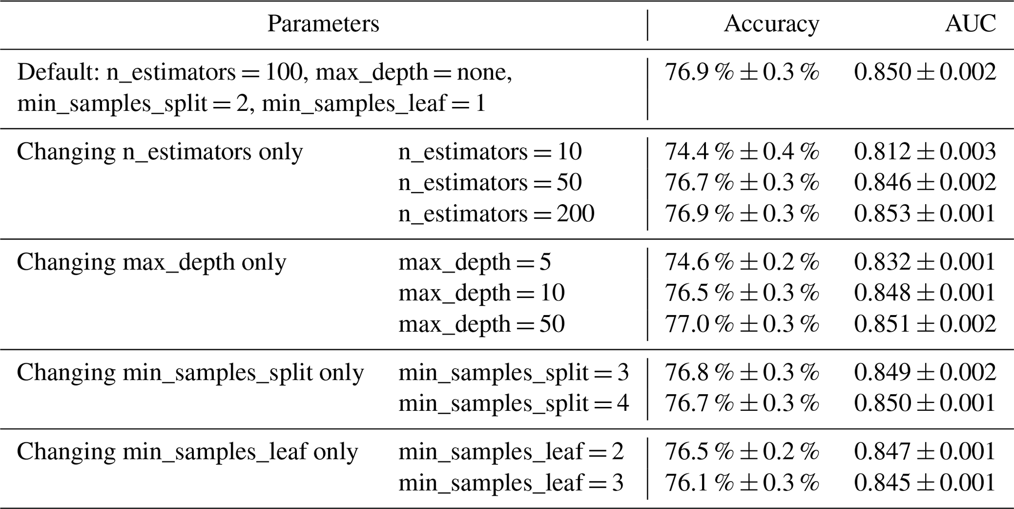
Ten-fold cross-validation is a resampling procedure commonly used to evaluate ML models. First, the dataset is shuffled randomly and split into 10 groups, which is a necessary step. Nine of the groups are used for training and the other group for evaluation. In this application, we predict the occurrence of lightning (“Yes” vs. “No”) using nine training groups and evaluate the prediction using the remaining group. The RepeatedStratifiedKFold classifier includes multiple adjustable parameters, including the number of trees (n_estimators, defaults to 100) and the maximum depth of the tree (max_depth, defaults to “none”). Setting the maximum depth to “none” ensures that the nodes are expanded until all leaves are pure or until all leaves contain less than min_samples_split (defaults to 2) samples, which is the minimum number of samples required to split an internal node. The parameter min_samples_leaf (defaults to 1) is the minimum number of samples required to be at a leaf node. We tried each parametrization option in Table 1 50 times but found that the default parameters provided the best or nearly best performance. Since random shuffling can affect the performance, we have chosen to retain the default parameters. Our model only simulated the convective hours over the SGP, when convective clouds are detected from the ARM SGP site, which will not cause temporal auto-correlation since convective clouds do not occur frequently (817 h in total among nine summers).

3.1 Area under the curve (AUC) calculation

The receiver operating characteristic (ROC) curve was first used in signal detection theory to represent the trade-off between hit rates and false alarm rates (Green and Swets, 1966). For a ML classifier model, a positive or negative prediction for a certain threshold will be made for a given set of input variables. A confusion matrix is then made that records the frequency of true positive (TP), false positive (FP), false negative (FN) and true negative (TN) predictions. The true positive rate (TPR, TPR = TP$/$(TP + FN)) and false positive rate (FPR, FPR = FP$/$(FP + TN)) can be calculated accordingly. TPR and FPR vary with threshold, and we can put (FPR, TPR) points on the ROC space as the threshold changes. Both FPR and TPR range in value from 0 to 1, and we connect the points to get an ROC curve. The area under the ROC curve integrating from 0 to 1 is called AUC, which measures the discriminatory power of the predictive classification model.

3.2 Random forest classifier and 10-fold cross-validation

The random forest classifier is an ensemble learning method for classification that operates by constructing a multitude of decision trees at training time. For classification tasks, the output of the random forest is the class selected by the most trees.

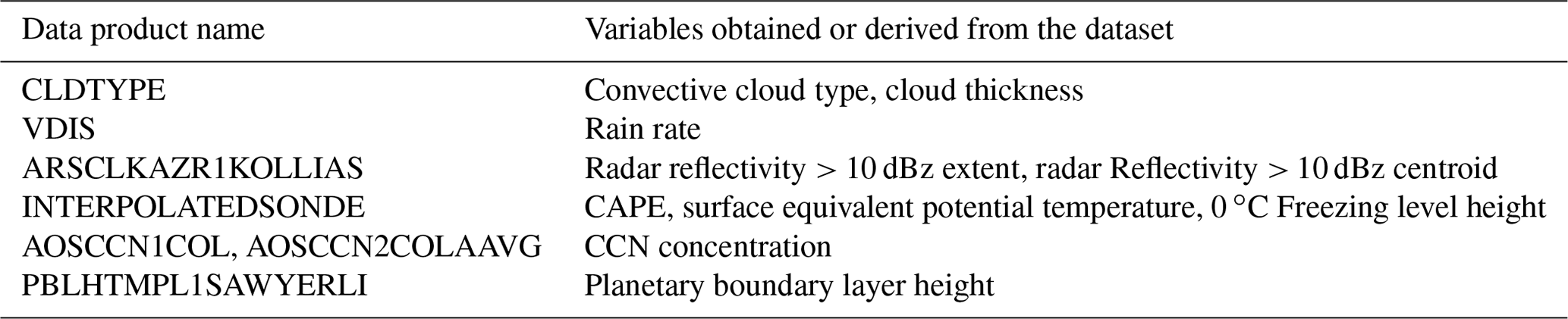
Table 2 Datasets containing the variables considered for use in the lightning parameterization.

3.3 ARM dataset processing

Cloud top height, cloud base height and cloud type are obtained from the CLDTYPE data product with a temporal resolution of 1 min. For the SGP site, deep convective clouds are identified as clouds with a cloud base height lower than 3.5 km and a cloud top height higher than 6.5 km (Flynn et al., 2017). We use this product to identify convective clouds and calculate the convective cloud thickness from the cloud base to the cloud top. For each hour, the variable “cloud thickness” is obtained by averaging thicknesses for each minute during the hour with convective clouds. Rain rate is measured with a temporal resolution of 1 min (Bartholomew, 2016) and is contained in the VDIS (Video Disdrometer) product. The variable “rain rate” is the hourly sum. The ARSCLKAZR1KOLLIAS data product provides us with zenith-pointing radar reflectivity profiles at the Ka band (35 GHz) every 4 s with a vertical resolution of 30 m. According to Seo and Liu (2005), the relationship between radar reflectivity and ice water content for the six ice particle types near the ARM SGP site shows that the ice water content for each vertical layer is proportional to the 0.79th power of radar reflectivity. We have set a threshold of 10 dBz for layers, so that each layer will have at least 0.5 g m⁻³ ice water content when its radar reflectivity exceeds this threshold. We only take measurements of radar reflectivity at altitudes higher than 3 km as temperatures at altitudes lower than this are always too low to support ice in clouds during the summer at the ARM SGP site. The hourly average extent and centroid of radar reflectivity exceeding 10 dBz are recorded as the variables “radar reflectivity > 10 dBz extent” and “radar reflectivity > 10 dBz centroid”, respectively. These variables are chosen because they are closely associated with mixed-phase cloud extent and height. Fifty-four environmental variables (Jensen et al., 1998) are measured every minute and recorded in INTERPOLATEDSONDE. We primarily use the profiles of pressure, temperature and dew point and calculate the meteorological variables listed in Table 2 for this product. We use the 30th minute profile of the hour to calculate these variables, except for CAPE. We calculate the average CAPE based on the 15th minute and 45th minute profiles of the hour. We do not calculate values for each minute due to computational expense. The AOSCCN1COL and AOSCCN2COLAAVG datasets include cloud CCN concentrations every minute. We use both datasets because the AOSCCN1COL dataset ended in September 2017 and the AOSCCN2COLAAVG dataset started from April 2017. The datasets both measure the CCN concentrations at different supersaturation levels by manipulating the supersaturation in the instruments from 0.1 % to 1.2 %, although there are some minor changes in technique. According to Politovich and Cooper (1988), the maximum supersaturation is usually smaller than 0.5 % in cumulus clouds. Thus, we have selected all the CCN concentration measurements at supersaturation in the range from 0.4 % to 0.6 % and calculated the average value for each hour. Measurements of the planetary boundary layer height (PBLH) are conducted every 30 s using micropulse lidar (MPL) and recorded in PBLHTMPL1SAWYERLI. We take the average values of the PBLH for each hour and record them as the variable “PBLH”.

Because of the differences in temporal resolution and formatting, each variable from the ARM SGP site is merged into a database at a temporal resolution of 1 h (Table 2).

4 Results

4.1 ML-based investigation of the variables affecting lightning occurrence

First, we identified convective hours using the CLDTYPE product at the ARM SGP site. This product provides an automated cloud type classification based on microphysical quantities derived from vertically pointing lidar and radar. Twenty-four hours were checked each day.

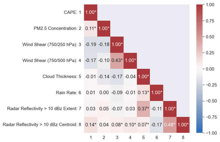
Figure 1 Pearson correlation coefficients between variables selected for use in the ML analysis. Asterisks indicate that the correlations are significant at the 95 % level. The relatively low correlations between the pairs make them good candidates for the analysis.

Numerous meteorological variables were considered for use in the ML-based analysis. Eight mostly independent variables (i.e., variables with inter-correlations |R| of 0.5 or less) were selected for further analysis. These variables and their inter-correlations are shown in Fig. 1. In total, there were 817 h with detectable deep convective clouds and measurements of all eight variables available during JJAS of 2012–2020. Lightning was observed in the 1^∘ × 1^∘ grid box (36–37^∘ N, 97–98^∘ W) encompassing the ARM site in 509 of those hours.

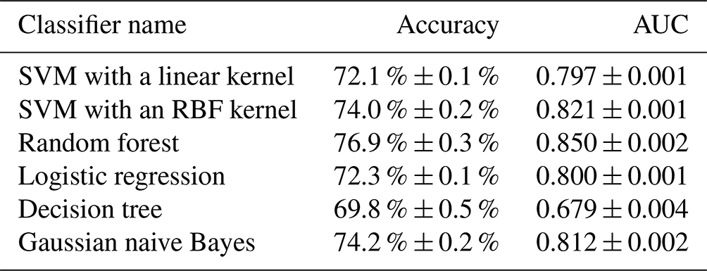
In addition to the random forest method, five other ML classifier schemes were tested. The support vector machine (SVM) algorithm fits a hyperplane in space. The dimensions of the hyperplane are equal to the number of features. This approach results in a distinct classification of data points by using different kernels containing a set of mathematical functions to massage the data. Linear and radial basis function (RBF) kernels are two different kernels used in the SVM. Logistic regression is a classification algorithm used to predict a binary outcome based on a set of independent variables and the sigmoid function. A decision tree is a tree-like structure where each internal node tests an attribute, each branch corresponds to an attribute value and each leaf node represents the final decision or prediction. Gaussian naive Bayes is based on the probabilistic approach and Gaussian distribution, which assume that each parameter has an independent capacity to predict the output variable. Our goal is to use the eight input variables to predict the occurrence of lightning in a convective hour. We repeat 10-fold cross-validation 50 times in order to estimate the overall performance of different ML models. Based on our 50 simulations with the 10-fold cross-validation, the random forest classifier was identified as the best classifier among the common classifiers shown below because of its highest accuracy and its AUC value (Table 3).

Table 3 Mean accuracy and AUC with the standard deviation for each ML classifier method. Each method was run 50 times using 10-fold cross-validation. The accuracy is defined as the ratio of correct predictions of lightning occurrence (“Yes” vs. “No”) to total predictions. AUC provides an aggregate measure of performance across all the classification thresholds and can have values ranging from 0.5 to 1.0. Models with higher values of AUC do a better job of distinguishing between convective hours with and without lightning.

After choosing the random forest classifier model, we split the dataset randomly into training and test sets with split percentages of 75 % to 25 % and performed 1000 simulations with the random forest classifier to evaluate its overall performance, as shown in the confusion matrix (Table 4). This classifier predicts lightning occurrence with an accuracy of 77 % using these eight input variables.

Table 4 This confusion matrix shows the accuracy of the random forest classifier. The frequency (percentage and standard deviation) of the binary prediction that fell into each of the four categories is shown. The overall accuracy, which is sum of the true negatives (24.5 %) and the true positives (52.1 %), is about 77 %.

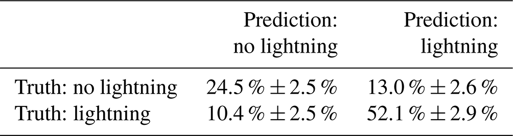
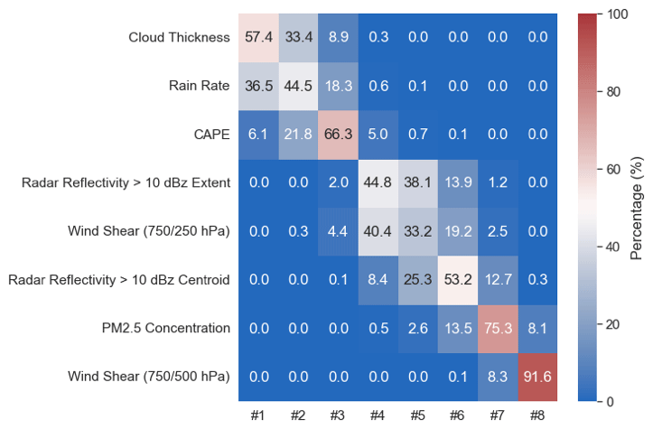
Figure 2 Variable importance ranking distribution. Probability distribution function showing the frequency at which each variable was rated from most to least important after running the random forest classifier with random splitting 1000 times.

In addition to the confusion matrix, an overall ranking of feature importance is also generated from the ML model, as shown in Fig. 2. The feature importance is a measure of how much one variable decreases the impurity, i.e., the probability that more than one class of data will remain in a node after processing through various decision trees in the forest. This figure shows the percent of the 1000 simulations where each variable was identified as the most important feature (column no. 1) to the least important feature (column no. 8). For example, the variable “cloud thickness” was identified as the most important feature in 57.4 % of the 1000 runs, while it is the second (no. 2), third (no. 3) and fourth (no. 4) most important feature in 33.4 %, 8.9 % and 0.3 % of the runs. From the ranking distribution, we can identify that “cloud thickness”, “rain rate” and “CAPE” are the top three most important variables determining lighting occurrence in the model. The sum of the first-, second- and third-place percentages for each of these variables exceeds 90 %. The next three most important variables are radar reflectivity > 10 dBz extent, “wind shear (750 / 250 hPa)” and radar reflectivity > 10 dBz centroid. The least important variables are “PM_2.5 concentration” and “wind shear (750 / 500 hPa)”. The low sensitivity to PM_2.5 concentrations could be due to its small range of variability, especially compared with other variables' relatively large variations. The differentiation of the variables into the most important, modest and least important categories is distinct according to the robust ranking distribution, as can be seen in Fig. 2. The importance of the variables can also be estimated by removing them from the model and seeing how successful the remaining variables are at predicting the true outcome. In Sect. 3.2, our model was found to have an overall accuracy of 76.9 % and an AUC of 0.850. By removing “cloud thickness”, “rain rate” and “CAPE” separately, the accuracy dropped from 76.9 % to 72.1 %, 75.6 % and 74.3 %, and the AUC dropped from 0.850 to 0.797, 0.830 and 0.821. The impact of removing the other variables was smaller. Based on these metrics, the “cloud thickness” is the most important, followed by “rain rate” and then “CAPE”.

4.2 Contrast in meteorological variables between no-lightning and frequent-lightning hours in strong convective environments

ML provides robust feature importance rankings, which are useful for determining the importance of each variable. To aid in physical interpretation, we compare the meteorological variables' difference with or without the existence of lightning. In convective hours with lightning, the hourly flash count distribution is shown in Fig. 3. The average and median numbers of ENTLN flashes per hour in the 1^∘ × 1^∘ grid box containing the SGP site are 864.9 and 162.5, respectively, with the large difference indicating that the distribution is skewed by hours with very frequent lightning.

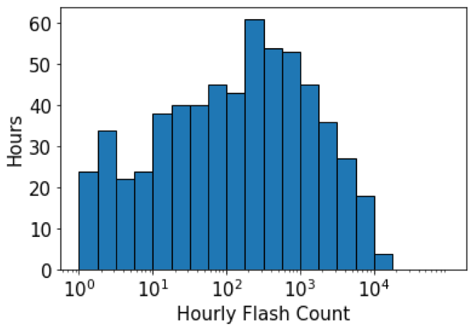
Figure 3 Hourly flash count distribution for flashing hours in the 1^∘ × 1^∘ grid box containing the SGP site. Note that the x axis is logarithmic. There are 608 h with both flashes and convective clouds detected, accounting for 2.3 % among all 26 352 h in the summer months (June, July, August and September) from 2012 to 2020.

To ensure that the environment is favorable for lightning, we have set a threshold of CAPE = 2000 J kg⁻¹ and only selected hours with convective clouds when CAPE is larger than 2000 J kg⁻¹, where 2000 J kg⁻¹ is chosen as the threshold for a strong convective environment following several studies (Rutledge et al., 1992; Chaudhuri, 2010; Chaudhuri and Middey, 2012; Hu et al., 2019). Overall, there were 175 h satisfying the CAPE threshold. Of these hours, 41 had no lightning in a 3 h period centered on the CAPE observation and were labeled “no-lightning hours”. Seventy-five of the hours had 3 h mean flash rates exceeding the median flash rate of 162.5 and were classified as “frequent-lightning hours”, while the remainder of the hours (59) were deemed intermediate lightning hours.

Table 5 The contrast (mean, standard deviation and significance of difference) in meteorological variables put into the ML random forest model between no-lightning and frequent-lightning hours. For example, a p value of < 0.01 indicates that the difference is significant at the 99 % level.

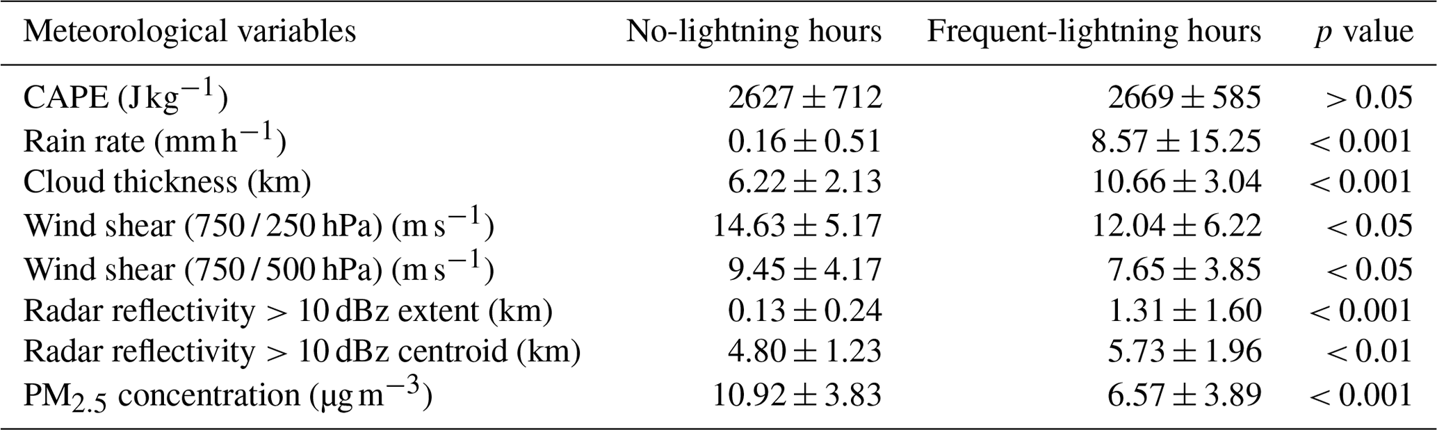
Table 6 The contrast (mean, standard deviation and significance of difference) in aerosol-related variables between no-lightning and frequent-lightning hours.

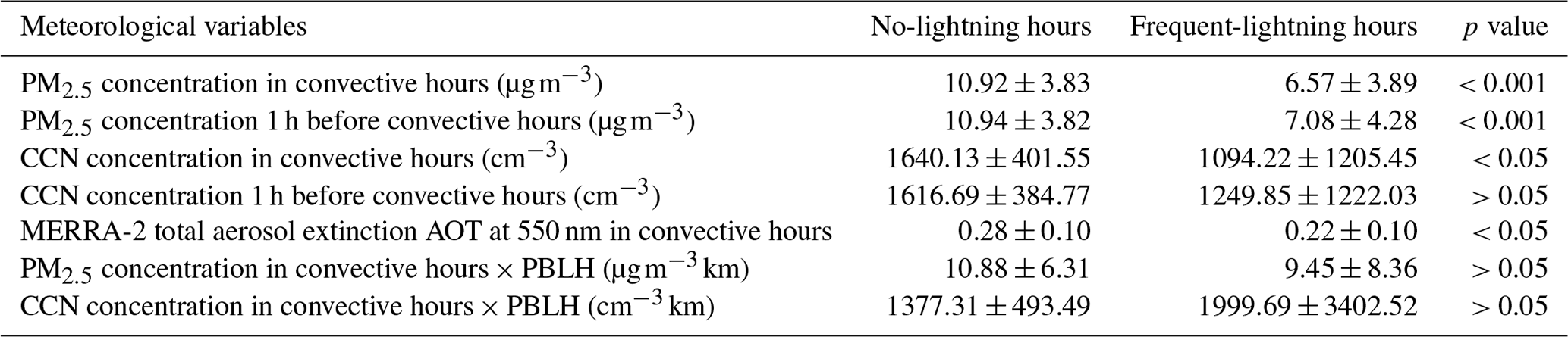
The contrast in meteorological variables between the no-lightning and frequent-lightning hours is shown in Table 5.

After limiting the analysis to hours with CAPE > 2000 J kg⁻¹, we do not see a significant difference in CAPE between the no-lightning and frequent-lightning hours, indicating that once CAPE reaches a high value, it is no longer a good predictor of lightning occurrence. The rain rate and convective cloud thickness are much larger when lightning is frequent (p value less than 0.001), indicating that lightning is associated with high rain rates and deep convective clouds. This finding is consistent with the ML results. The radar reflectivity > 10 dBz extent variable is an order of magnitude larger when lightning occurs, indicating that the total ice water path, which is associated with high values of radar reflectivity, is also much higher. In addition, the centroid altitude of radar reflectivity is higher by about 19 %, a difference that is significant at the 99 % confidence interval (CI). Mean vertical wind shear is smaller when flashes are present, with decreases of about 18 % in 750 to 250 hPa shear (significant at the 95 % CI) and 20 % in 750 to 500 hPa shear (significant at the 95 % CI). Perhaps surprisingly, differences in PM_2.5 between the non-flashing and frequent-flashing hours are significant. Specifically, hours with frequent lightning have 40 % less PM_2.5 than no-lightning hours. This result is seemingly inconsistent with the ML analysis discussed earlier, which showed that PM_2.5 had little effect on lightning occurrence and with previous studies finding that enhanced lightning activity is related to higher aerosol loading.

CCN concentrations are also more than 30 % smaller during frequent-lightning hours than no-lightning hours (Table 6). Similarly, values of MERRA-2 total aerosol extinction AOT at 550 nm simultaneous with the convective hour are lower in frequent-lightning hours than in no-lightning hours (significant at the 99 % CI). One plausible explanation for this is aerosol wet removal, given the fact that lightning occurrence is closely related to precipitation. Therefore, we examined the PM_2.5 and CCN concentrations during the convective hour and also during the hours preceding the convective hour, as shown in Table 6. During all these hours, we still notice less PM_2.5 concentration when flashes are frequent, but differences in CCN concentrations are small and insignificant statistically.

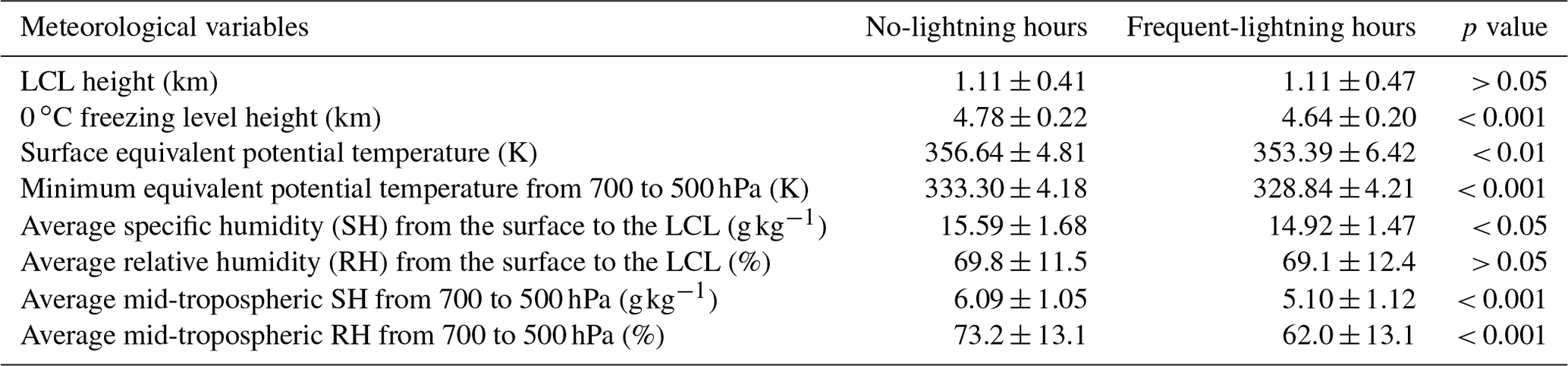
Table 7 The contrast (mean, standard deviation and significance of difference) between no-lightning and frequent-lightning hours in variables derived from the INTERPOLATEDSONDE data product.

Another possible explanation is mixing of pollutants throughout the planetary boundary layer (PBL). A higher PBLH is associated with greater vertical mixing and often a larger CAPE and higher surface temperature (Zhang et al., 2013). Sun and Liang (2020) found that higher PBLHs were common during extreme precipitation. Both higher CAPE and higher precipitation rates are related to lightning occurrence. We calculated the product of the PBLH and the PM_2.5 or CCN concentration, assuming that pollutants are distributed homogeneously within the PBL, and compared the values between no-lightning and frequent-lightning hours. Even though the differences in the product of the CCN concentration and the PBL height between the no-lightning and frequent-lightning periods were nearly 50 %, the differences were insignificant at the 95 % CI due to large variability. Thus, mixing through a deeper PBL could be the cause of the differences in PM_2.5 and CCN concentrations.

Some additional meteorological variables are calculated from the INTERPOLATEDSONDE dataset at the ARM SGP site. This value-added product provides us with profiles of pressure, temperature and dew point. The contrast of these meteorological variables between no-lightning and frequent-lightning hours is shown in Table 7.

According to the table, the LCL height and vertically integrated relative humidity (RH) from the surface to the LCL do not vary between no-lightning and frequent-lightning hours. These variables affect warm-cloud depth (Medina et al., 2022). Differences in the height of the 0 ^∘C freezing level (0.14 km), mean specific humidity (SH) from the surface to the LCL (0.67 g kg⁻¹) and surface equivalent potential temperature (3.25 K) are relatively small but significant statistically. The mid-tropospheric SH and RH are much lower during hours with thunderstorm activity (0.99 g kg⁻¹, 11.2 %, respectively), which is consistent with the analysis of convective profiles in the Amazon by Wall et al. (2014). They speculated that the increased lapse rate of humidity associated with a dry mid-troposphere increased the lapse rate of equivalent potential temperature and increased the severe storm threat when abundant moisture was present in the lower troposphere. Finally, the minimum equivalent potential temperature in the mid-troposphere is lower in frequent-lightning hours (4.46 K), which is consistent with Scala et al. (1990), who found that cells with a less pronounced equivalent potential temperature minimum are less likely to produce vigorous vertical transport than those developing in environments with a relatively strongly pronounced minimum. The low equivalent potential temperature region is considered a source of cool dry air which feeds penetrating downdrafts, helping to maintain an intense storm (Pickering et al., 1993).

4.3 The IC flash fraction relationship with $\sqrt{\mathrm{CAPE}}$

Holton (1973) found that CAPE plays an important role in determining the maximum parcel updraft velocity, which is proportional to $\sqrt{\mathrm{CAPE}}$ based on parcel theory. We have noticed a positive relationship between the IC fraction and $\sqrt{\mathrm{CAPE}}$, as shown in Fig. 4. This analysis is based on 304 h with convective clouds detected at the ARM SGP site from the CLDTYPE product and plentiful flashes (hourly flash count > median value of flashes during convective hours = 162.5, which does not have the same definition with frequent-lightning hours in Sect. 4.2) to ensure that the statistics are meaningful.

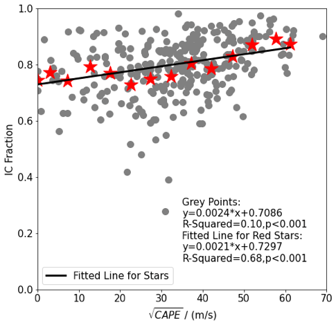
Figure 4 The relationship between the IC fraction and $\sqrt{\mathrm{CAPE}}$. The grey points show the IC fraction for convective hours with plentiful flashes, while the red stars show the mean IC fraction for 5 m s⁻¹ $\sqrt{\mathrm{CAPE}}$ bins. The fitted line for the binned data and its equation are shown in the figure.

From Fig. 5, as $\sqrt{\mathrm{CAPE}}$ increases from 0 to 60 m s⁻¹, the IC fraction increases from 0.7 to about 0.9. A hypothesis for the relationship is that the higher $\sqrt{\mathrm{CAPE}}$ represents a stronger convective environment with stronger updrafts. The stronger updrafts bring the electrification zone further above the surface, resulting in fewer flashes reaching the surface and consequently a greater IC flash fraction. This hypothesis is supported by the fact that higher IC flash fractions are associated with higher IC heights, as shown in Fig. 5. This relationship has not been widely discussed in previous studies, as they have focused on land–ocean contrast (Lapp and Saylor, 2007) or cloud vertical development (Williams et al., 1989). We tested that association between the $\sqrt{\mathrm{CAPE}}$ and IC fraction using a chi-square calculator for a 2 × 2 contingency table and found that the relationship was significant at p < 0.001.

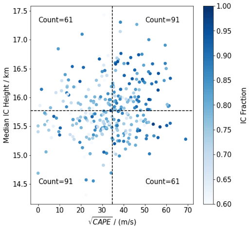
Figure 5 IC height and fraction with $\sqrt{\mathrm{CAPE}}$. Median IC height is plotted against the $\sqrt{\mathrm{CAPE}}$ for hours when flash rates exceed the median of flashing hours. The intensity of the colors shows the fraction of flashes that are IC. The dashed lines show the median value of $\sqrt{\mathrm{CAPE}}$ and IC height, respectively. The counts were used in the chi-square calculator and show the number of data points in each region of the figure.

Price and Rind (1993) found that the ratio of CG to IC lightning is related to the cold-cloud thickness rather than the height of the freezing level. The cold-cloud thickness method has been applied to models to estimate the production of nitrogen oxides by lightning (e.g., Price and Rind, 1994; Goldberg et al., 2022; Pérez-Invernón et al., 2023). The relationship found here between the CG fraction and $\sqrt{\mathrm{CAPE}}$ when verified with additional lightning datasets over a broader area would provide an alternative approach for parameterizing the ratio of CG to IC lightning in chemistry and climate models.

5 Conclusion

Previous ML-based studies of lightning frequency focus on larger regions, have a coarser time resolution, or focus on CG lightning only. Here, we take advantage of rich measurements of atmospheric and cloud properties at the ARM SGP site and ENTLN flash counts to explore the factors affecting flash rates at an hourly time resolution using ML models. We limit the analysis to hours when convective clouds are detected at the SGP site and then nowcast the occurrence of lightning and examine the conditions under which lightning occurs. We begin by inputting eight mostly independent meteorological variables into a random forest ML model to predict lightning occurrence. The ML model has an accuracy of more than 76 % and an AUC of 0.850, and the top, middle and least important variables' sorting is significant according to the robust ranking distribution. The most important variables affecting lightning occurrence turn out to be cloud thickness, rain rate and CAPE.

In strong convective environments (CAPE > 2000 J kg⁻¹), several variables, including rain rate and cloud thickness, vary significantly between no-lightning and frequent-lightning periods. In addition, our analysis indicates that values of mid-tropospheric humidity are typically lower during frequent-flashing hours, with low values of mid-tropospheric humidity indicative of greater convective instability. Both the 0 ^∘C freezing level height and the surface equivalent potential temperature have small but statistically significant differences between no-lightning and frequent-lightning hours. Minimum equivalent potential temperatures in the mid-troposphere are typically 4.46 K lower in frequent-lightning hours, suggesting that a source of cool dry air from penetrating downdrafts is helpful for maintaining intense storms.

A positive relationship is found between $\sqrt{\mathrm{CAPE}}$ and IC fraction in convective hours with plentiful flashes, which can provide models with another alternative parameterization option of the ratio of CG to IC. This may be explained by the fact that a higher $\sqrt{\mathrm{CAPE}}$ represents a stronger convective environment, which can bring the electrification zone further above the surface, resulting in a greater IC flash fraction. This hypothesis is supported by the variation in median IC heights with $\sqrt{\mathrm{CAPE}}$, although more analysis is needed to confirm the preliminary finding due to uncertainties in IC heights from ENTLN and the limited sample size. Lightning Mapping Array (LMA) data with more accurate flash heights could be used together with ENTLN flash type information to verify the positive relationship between $\sqrt{\mathrm{CAPE}}$ and IC fraction.

As lightning processes are complicated, better time resolution is needed to better understand the mechanism. This study focuses on hourly time resolution. ML can provide a quick and efficient result when dealing with multiple variables, while subsequent analysis and discussion are essential for understanding the physical meaning behind the result. This study only focuses on the region around the ARM SGP site, and we simply assumed that those measurements are representative of the entire 1^∘ × 1^∘ grid, which adds uncertainty because the scale of convection is typically smaller than this. Future analysis over other regions is desired to enrich the data volume in order to train the ML model and get more reliable and robust results.