the Creative Commons Attribution 4.0 License.
the Creative Commons Attribution 4.0 License.
 | 24 Nov 2023
Dynamics-based estimates of decline trend with fine temporal variations in China's PM2.5 emissions
Zhen Peng
Lili Lei
Zhe-Min Tan
Aijun Ding
Xingxia Kou
Timely, continuous, and dynamics-based estimates of PM2.5 emissions with a high temporal resolution can be objectively and optimally obtained by assimilating observed surface PM2.5 concentrations using flow-dependent error statistics. The annual dynamics-based estimates of PM2.5 emissions averaged over mainland China for the years 2016–2020 without biomass burning emissions are 7.66, 7.40, 7.02, 6.62, and 6.38 Tg, respectively, which are very closed to the values of the Multi-resolution Emission Inventory (MEIC). Annual PM2.5 emissions in China have consistently decreased by approximately 3 % to 5 % from 2017 to 2020. Significant PM2.5 emission reductions occurred frequently in regions with large PM2.5 emissions. COVID-19 could cause a significant reduction of PM2.5 emissions in the North China Plain and northeast of China in 2020. The magnitudes of PM2.5 emissions were greater in the winter than in the summer. PM2.5 emissions show an obvious diurnal variation that varies significantly with the season and urban population. Compared to the diurnal variations of PM2.5 emission fractions estimated based on diurnal variation profiles from the US and EU, the estimated PM2.5 emission fractions are 1.25 % larger during the evening, the morning peak is 0.57 % smaller in winter and 1.05 % larger in summer, and the evening peak is 0.83 % smaller. Improved representations of PM2.5 emissions across timescales can benefit emission inventory, regulation policy and emission trading schemes, particularly for especially for high-temporal-resolution air quality forecasting and policy response to severe haze pollution or rare human events with significant socioeconomic impacts.
- Article
(7428 KB) - Full-text XML
-
Supplement
(450 KB) - BibTeX
- EndNote


Anthropogenic emissions have imposed essential influences on the Earth system, from hourly air quality and human health to long-term climate and environment. To reduce anthropogenic emissions, the Chinese government has enforced the Clean Air Action (2013) since 2013 (China State Council, 2013). Studies to date that evaluated the emission controls and understood the climate responses to emission reductions have often used either a fixed meteorology with emission changes or vice versa (Li et al., 2019, 2021; Zhai et al., 2021). Estimated emissions from empirical extrapolation were commonly applied to analyse the meteorological–chemical mechanisms and associated social–economic impacts from occasional events like the 2015 China Victory Day Parade and Coronavirus Disease 2019 (COVID-19) pandemic (Wang et al., 2017; Liu et al., 2020; Huang et al., 2020; Zhu et al., 2021). But to better understand both long-term and short-term influences from emission changes, the continuous, up-to-date, and high-temporal- and high-spatial-resolution emission estimates with coherent interactions of meteorology and emission changes are needed.
The complex contributions from energy production, industrial processes, transportation, and residential consumptions have imposed great challenges on accurately estimating the emissions. The emission inventories created by the traditional bottom-up techniques were typically outdated compared to the present day due to the lack of accurate and timely statistics, and they often used coarse temporal resolutions, from monthly to annual (Zhang et al., 2009; Li et al., 2014; Janssens-Maenhout et al., 2015b; Zheng et al., 2018). Alternatively, up-to-date emission estimates with high temporal and spatial resolutions could be provided by top-down techniques (Miyazaki et al., 2017), but most emissions estimated by top-down techniques were intermittent and analysed at monthly scales or longer (Zhang et al., 2016; Jiang et al., 2017; Qu et al., 2017; Cao et al., 2018; Müller et al., 2018; Chen et al., 2019; Li and Wang, 2019; Miyazaki et al., 2020). Moreover, emissions updated by the top-down techniques based on satellite observations could be insufficient to capture realistic near-surface characteristics (Li and Wang, 2019; Liu et al., 2011; Choi et al., 2020).
Given the development of observation networks and advanced data assimilation strategies, timely and dynamics-based emission estimates with high temporal resolutions can be achieved by harmonically constraining the atmospheric–chemical model with dense observations of trace gas compounds through an optimal assimilation methodology. The ensemble Kalman smoother (EnKS) (Whitaker et al., 2002; Peters et al., 2007; Peng et al., 2015), as a four-dimensional (4D) assimilation algorithm, makes use of chemical observations from the past to the future to provide an optimal estimate of source emissions, and it can capture the “error of the day” and construct fine emission characteristics with high temporal and spatial resolutions by using short-term ensemble forecasts (Kalnay, 2002). Since 2013, the fine particulate matter pollution (PM2.5, particles smaller than 2.5 µm in diameter) as the most urgent threat to public health has persistently decreased, and ground-based observations of PM2.5 have progressively increased (Huang et al., 2018). Thus, by harmonically assimilating dense surface PM2.5 observations into an atmospheric–chemical model through an EnKS, hourly estimates of PM2.5 emissions that were continuously cycled for the years 2016–2020 are presented in this study.
The timely estimated emissions can provide guidance for emission inventories that usually have time lags and emission trading schemes that often require up-to-date source emissions. Based on the dynamics-based estimated emissions with harmonic combination of the model and observations, a better evaluation of the emission controls and a more comprehensive understanding of the consequent climate responses can be obtained. The high-temporal-resolution estimated emissions can reveal features of emissions that are absent from the traditional ones with coarse temporal resolutions. Moreover, the timely and dynamics-based emission estimates with high temporal resolutions are essential for regional air quality modelling, especially for the occurrence of severe haze pollution, associated with timely evaluations of the impact on public health (Attri et al., 2001; Wang et al., 2014; Ji et al., 2018; Wang et al., 2020; Liu et al., 2021) and events that lead to large changes in emissions and significant socioeconomic impacts such as the COVID-19 pandemic (Huang et al., 2020; Le et al., 2020).
The estimate of PM2.5 emissions can be successfully constrained by the PM2.5 concentration observations through an ensemble Kalman filter (EnKF; Peng et al., 2017, 2018, 2020). For a retrospective reanalysis mode, here, all available PM2.5 concentration observations, including those data collected after the analysis time, can be used. Thus, an EnKS, a direct generalization of the EnKF, is applied to incorporate PM2.5 concentration observations both before and after the analysis time, aiming to provide an optimal estimate of the PM2.5 emission. In simple words, the emissions are updated by current and future observations though EnKS, while the concentrations are updated by current observations though EnKF. Detailed procedures of the EnKS are described in Sect. 2.1.
2.1 An ensemble Kalman smoother to update the source emission
The ensemble priors of source emissions ef is created by multiplying a scaling factor λf by the prescribed emission ep (Peng et al., 2017, 2018, 2020), where the superscript f denotes priors. Given a time-invariant ep, the update of ef is equivalent to the update of λf. Due to a time lag, the prior scaling factor at time t−1 () is updated by chemical observations at time t (). At time t−1, the prior scaling factor for the ith member is written as
The first term is the concentration ratio given by the prior of the chemical fields () normalized by the ensemble mean (), where β is an inflation factor used to compensate for the insufficient ensemble spread (Peng et al., 2017). Through using the concentration ratio, each ensemble member of the source emissions naturally has the spatial correlations given by the chemical fields. The second term is the mean of the posterior scaling factors at previous assimilation cycles, where the superscript a denotes posteriors, M is the length of smoothing, and the subscript indicates that the scaling factor at time j is updated by future observations from j+1 to t−1. The assimilation of future observations will be described below.
The ensemble square-root filter (EnSRF) (Peng et al., 2017) is used to update by assimilating . For the scaling factor at time t−1, the posterior ensemble mean is given by
and the posterior ensemble perturbations are given by
where denotes the background error covariance matrix of and ; indicates the background error covariance matrix of ; , , and are the observation forward operator, Jacobian matrix, and observation error covariance matrix of the chemical fields at time t; ρ is the localization matrix; and ∘ denotes the Schur (element-wise) product.
By applying the ensemble Kalman smoother (EnKS) (Whitaker et al., 2002; Peters et al., 2007), the chemical observation is also assimilated to update the posterior scaling factor at previous assimilation cycles . After assimilating the future chemical observation at time t, the posterior ensemble mean of the scaling factor at j is given by
and the posterior ensemble perturbations are given by
where denotes the background error covariance matrix of and . After Eqs. (2)–(5), the updated will be used to construct the prior scaling factor at the next time t+1.
As a Monte Carlo approach, the EnKS uses the forecast analysis error covariances based on ensemble forecasts and/or analyses to compute the Kalman gain matrix with time lags in order to incorporate observations from the past to the future. The first iteration of the EnKS is equivalent to the EnKF that assimilates observations up to the analysis time. The following iterations of EnKS assimilate observations in the future to update the state at the analysis time. The hourly forecasts of PM2.5 concentration from the cycling assimilation experiment matched the independent observed quantities (Fig. 1). Therefore, the ability of EnKS to retrieve the source emissions has been demonstrated. Previous studies also showed that simulations forced by the posterior emissions could produce improved forecasts for PM2.5, SO2, and NO2 compared to those produced with a priori emissions (Peng et al., 2020).
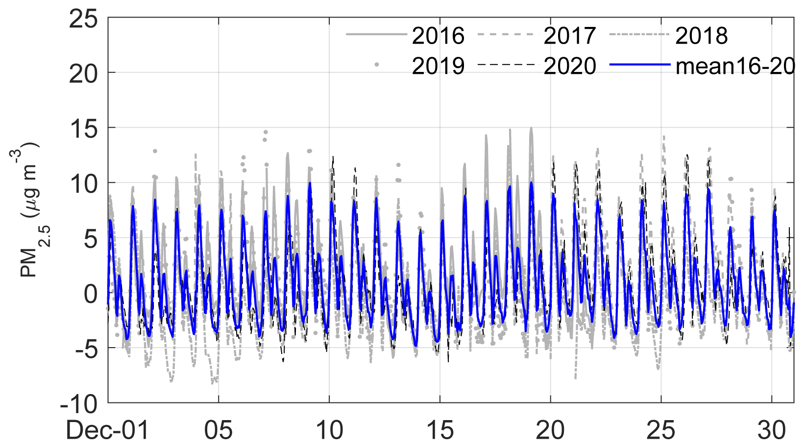
Figure 1Times series of hourly PM2.5 concentration biases (µg m−3). The ensemble mean priors compared to the observed quantities for December of the years 2016–2020 (grey and black) and the mean biases of the years 2016–2020 (blue).
2.2 WRF-Chem model, observations, and emissions
To simulate the transport of aerosol and chemical species, the WRF-Chem model version 3.6.1 (Grell et al., 2005) that has the meteorological and chemical components fully coupled is used. The model parameterization schemes follow Peng et al. (2017). Figure 2 shows the model domain that covers most east Asian regions. The horizontal grid spacing is 45 km, with 57 vertical levels and the model top at 10 hPa.
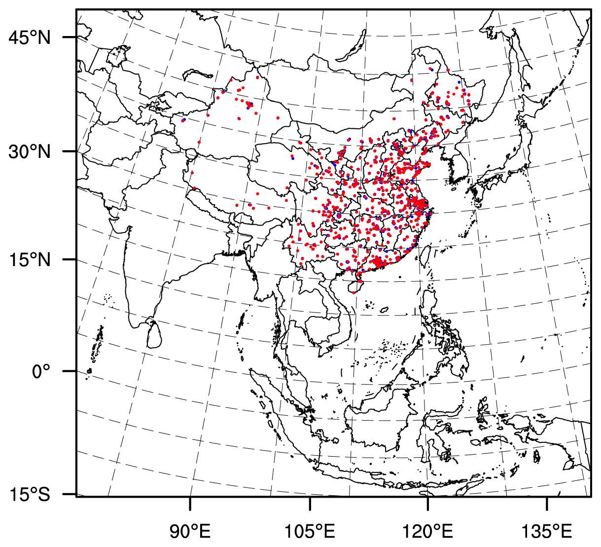
Figure 2Model domain and observation sites for cycling assimilation. Red and blue dots denote the assimilated and unassimilated observational sites, respectively.
Experiments are conducted for each year from 2016 to 2020 separately. The 6 h meteorological observations, including all in situ observations and cloud motion vectors from the National Centers for Environmental Prediction (NCEP) Global Data Assimilation System (GDAS; http://www.emc.ncep.noaa.gov/mmb/data_processing/prepbufr.doc/table_2.htm, last access: 6 November 2023), are assimilated every 6 h. The hourly observed chemical quantities, which contain PM10, PM2.5, SO2, NO2, O3, and CO from the Ministry of Ecology and Environment of China (https://aqicn.org/map/china/cn/, last access: 6 November 2023), are assimilated every hour. Figure 2 shows the assimilated chemical observation network, which has 560 randomly chosen stations from 1576 stations in total. The thinning of observations is applied to avoid correlated errors of observations. The spatial autocorrelation of the thinning of observations is close to the original observations (Peng et al., 2017). The observation priors are computed by the observer portion of the Grid-point Statistical Interpolation system (GSI) (Kleist et al., 2009).
The hourly and time-invariantly prescribed anthropogenic emissions are obtained from the EDGAR-HTAP (Emission Database for Global Atmospheric Research for Hemispheric Transport of Air Pollution) v2.2 inventory (Janssens-Maenhout et al., 2015b), in which the Chinese emissions are derived from the Multi-resolution Emission Inventory (MEIC) in 2010 (Lei et al., 2011; Li et al., 2014). Natural emissions, including the biogenic (Guenther et al., 1995), dust (Ginoux et al., 2001), dimethyl sulfide, and sea salt emissions (Chin et al., 2000), are computed online.
2.3 Assimilation and ensemble configurations
The PM2.5 emission directly gives the primary PM2.5 and then the primary PM2.5 along with other precursor emissions that could contribute to the secondary PM2.5. The observations of PM2.5 concentrations that contain both primary and secondary PM2.5 are used to constrain the PM2.5 emission through data assimilation. Thus, the correlations between the concentration observations and source emissions might be contaminated by the secondary PM2.5. Since the secondary formation process can be captured by the WRF-Chem model, the impact of the secondary PM2.5 is indirectly considered. The detailed updated state variables with the according observations follow Peng et al. (2018). The concentrations and emissions of PM2.5 and PM2.5 precursors (SO2 and NO) that have observations are updated by the observed quantities. Besides, NH3 concentrations and emissions are constrained by PM2.5 observations; however, the VOCs that are also PM2.5 precursors are not updated due to the lack of direct and limited observations. One possible way to untangle the impact of secondary PM2.5 on the estimates of PM2.5 emissions is to jointly estimate the source emission and the primary and secondary PM2.5 given the concentration observations.
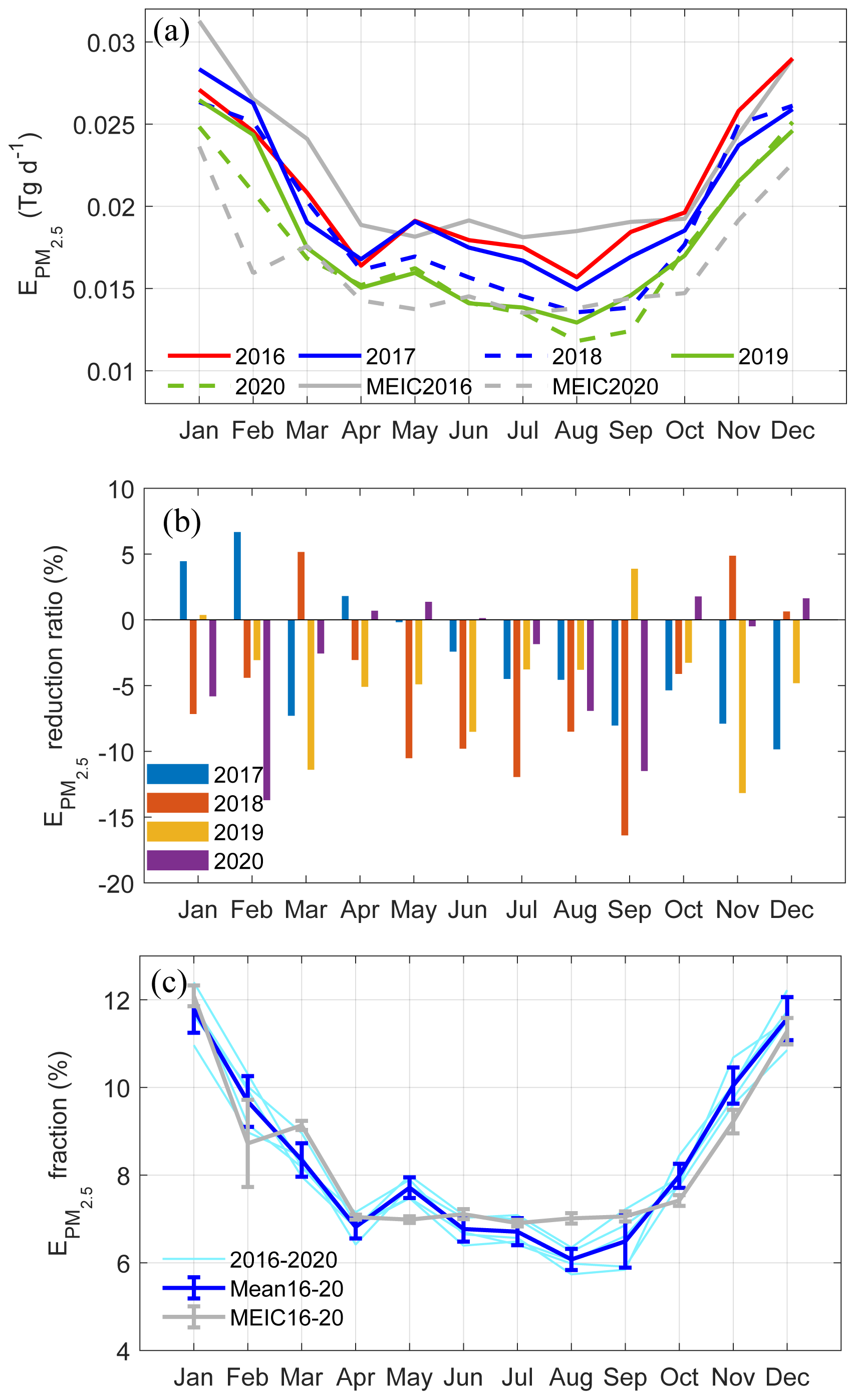
Figure 3(a) Dynamics-based monthly PM2.5 emission estimates (Tg d−1) summed over mainland China for each year from 2016 to 2020 (coloured) and the estimated PM2.5 emission from MEIC (grey). (b) Ratio of PM2.5 emission changes between two adjacent years from year 2016 to 2020 normalized by the PM2.5 emissions of the year 2016. (c) Monthly fractions of dynamics-based PM2.5 emission estimates for years 2016–2020 (light blue); the 5-year mean fractions of dynamics-based monthly PM2.5 emission estimates, with bars denoting 1 standard deviation of the 5-year variations (dark blue); and the monthly fractions of estimated PM2.5 emissions from MEIC (grey).
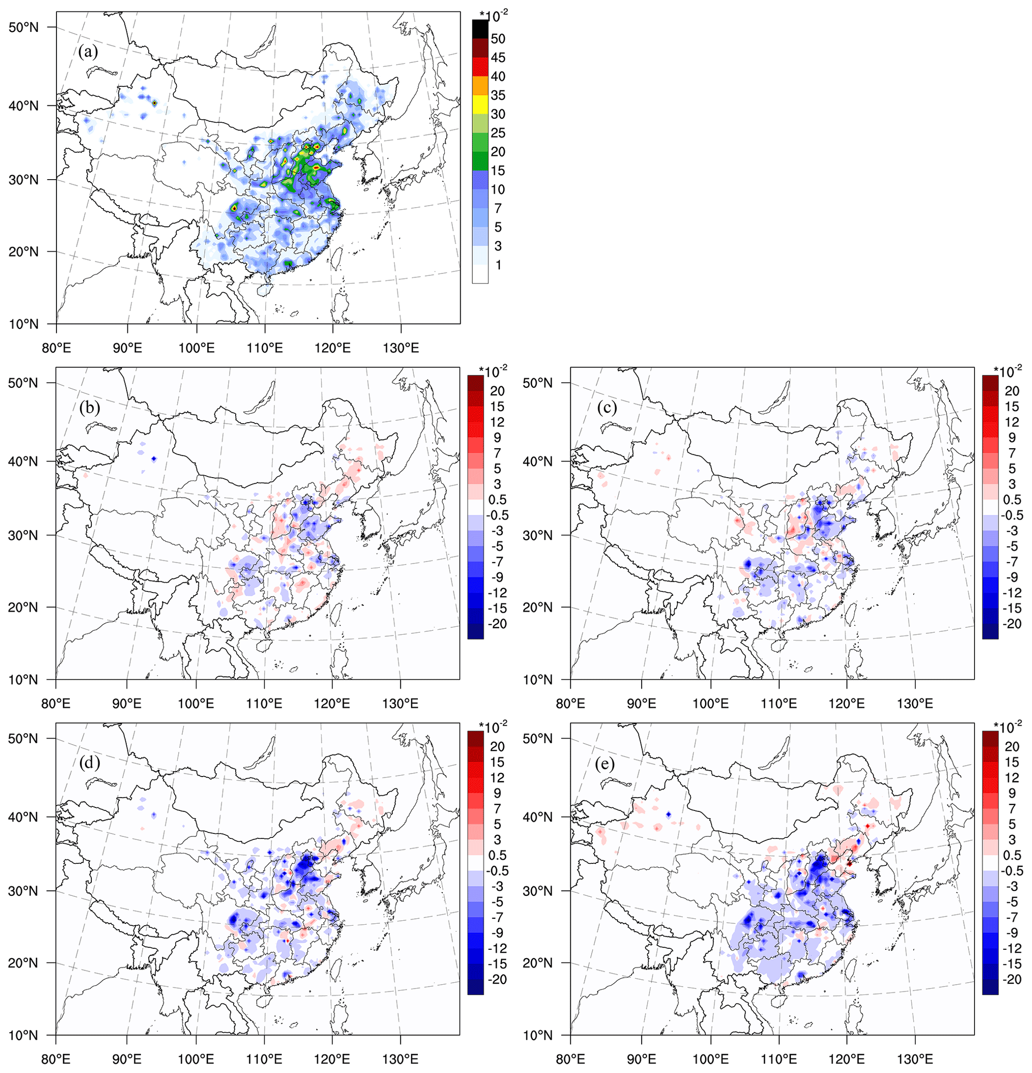
Figure 4(a) Spatial distribution of dynamics-based PM2.5 emission estimates (µg m−2 s−1) for the year 2016 and spatial distributions of dynamics-based PM2.5 emission changes for the years (b) 2017, (c) 2018, (d) 2019, and (e) 2020 compared to those of the year 2016.
The National Oceanic and Atmospheric Administration (NOAA) operational EnKF system (https://dtcenter.ucar.edu/com-GSI/users/docs/users_guide/GSIUserGuide_v3.7.pdf, last access: 6 November 2023), which is an EnSRF and is modified with the EnKS feature, is used to assimilate the observations. The ensemble size is set to 50. To combat the sampling error resulting from a limited ensemble size, covariance localization and inflation are applied. The Gaspari and Cohn (GC) (1999) function with a length scale of 675 km is used to localize the impact of observations and mitigate the spurious error correlations between observations and state variables. The constant multiplicative posterior inflation (Whitaker and Hamill, 2012), with a coefficient of 1.12 for all meteorological and chemical variables, is applied to enlarge the ensemble spread. The inflation β for advancing the scale factor is 1.2. The smoothing length M for source emissions is 4, and the EnKS lagged length K is 6. The larger the K value, the more future observations are assimilated to constrain the current emission estimate. But the sample estimated temporal correlations could be contaminated by sampling errors and model errors, especially with increased lagged times. Thus, there is a tradeoff between the amount of future observations and the accuracy of the sample estimated temporal correlations. The choice of K (=6) is determined by sensitivity experiments.
At 00:00 UTC on 26 December of the previous year, ensemble initial conditions (ICs) of the meteorological fields are generated by adding random perturbations that sample the static background error covariances (Barker et al., 2012) on the NCEP FNL (final) analyses (Torn et al., 2006). Ensemble ICs of the chemical fields are 0, and source emissions of each ensemble member are adopted from the EDGAR-HTAP v2.2 inventory with random perturbations of mean 0 and variances of 10 % of the emission values. Hourly ensemble lateral boundary conditions (LBCs) are generated using the same fixed-covariance perturbation technique as the ensemble ICs. After a 6 d spin up, ensemble data assimilation experiments start cycling for each year.
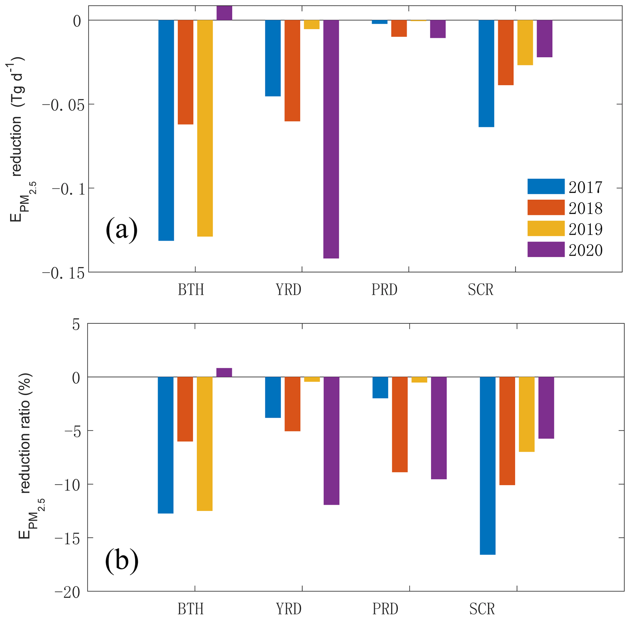
Figure 5(a) The differences in dynamics-based PM2.5 emission estimates between the years 2017–2020 and 2016 and (b) the differences normalized by the of year 2016.
Starting from the time-invariant source emission PR2010 (Janssens-Maenhout et al., 2015b), the dynamics-based estimates of the PM2.5 emissions are obtained, which include the contributions of both the anthropogenic and biomass burning emissions. The mean annual PM2.5 emissions from biomass burning in China (2003–2017) amounted to 0.51 Tg (Yin et al., 2019). The annual dynamics-based estimates of PM2.5 emissions (DEPEs) averaged over mainland China for the years 2016–2020 without biomass burning emissions are 7.66, 7.40, 7.02, 6.62, and 6.38 Tg, respectively. The values from the Multi-resolution Emission Inventory (MEIC; Zheng et al., 2018), which does not consider the contributions of biomass burning emissions, are 8.10, 7.60, 6.70, 6.38, and 6.04 Tg. Thus the annual DEPEs are very close to the values of MEIC. From 2017 to 2020, the estimated annual PM2.5 emissions are reduced by 3.4 %, 8.4 %, 13.6 %, and 16.7 % compared to that of year 2016. There has been a 3 %–5 % persistent reduction in annual PM2.5 emissions from the year 2017 to 2020, which demonstrates the effectiveness of China's Clean Air Action (China State Council, 2013), implemented since 2013, and China's Blue Sky Defense War Plan (2018), enforced since 2018 with strengthened industrial emission standards, phased out outdated industrial capacities, promoted clean fuels in residential sector, and so on (Zhang et al., 2019).
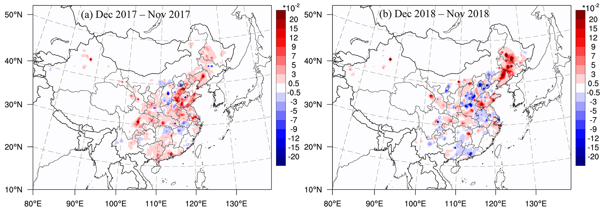
Figure 6Spatial distributions of dynamics-based PM2.5 emission changes in (a) December 2017 compared to November 2017 and (b) December 2018 compared to November 2018.
Table 1Dynamics-based PM2.5 emission estimates of the year 2016 for each province whose value is larger than 0.01 µg m−2 s−1 are shown in the second column. Ratios of PM2.5 emission changes for the years 2017–2020 compared to 2016 are shown from the third to the sixth column, with negative (roman)/positive (italic) values indicating a decrease/increase in PM2.5 emissions.
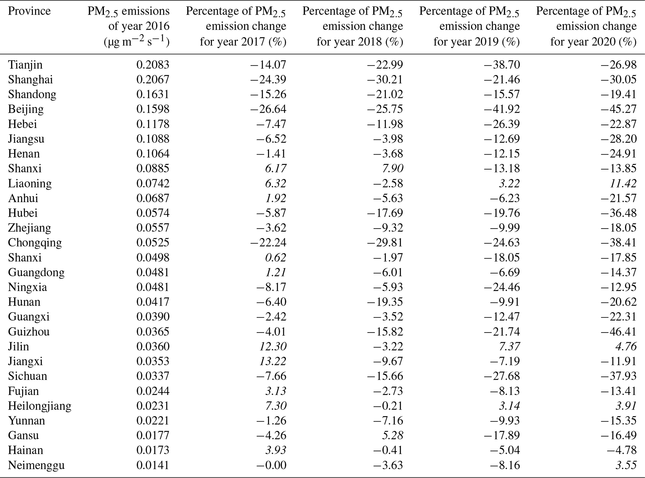
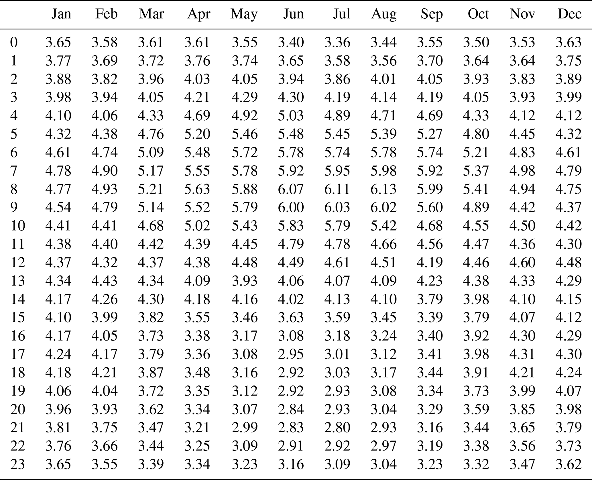
Table 2The 5-year mean diurnal fractions (%) of the dynamics-based PM2.5 emission estimates over mainland China in local solar time (LST) for each month.
The monthly DEPEs show reductions in PM2.5 emissions nearly every month from 2016 to 2020 (Fig. 3a), which further demonstrates the effectiveness of China's national plan. Compared to 2016, both the reduction amount and the reduction ratio of PM2.5 emission are more prominent for February, March, June–September, and November than the other months (Fig. 3b). Given larger magnitudes of PM2.5 emissions in winter than in summer, emission controls with a focus on October to May should be considered in the design of future clean-air actions in China since total PM2.5 emissions during period account for approximately 75 % of the annual amount. Spatial distributions of the changes in PM2.5 emissions from 2017 to 2020 compared to 2016 show that significant decreases occurred in the Beijing–Tianjin–Hebei region (BTH), the Yangtze River Delta region (YRD), the Pearl River Delta region (PRD), and the Sichuan–Chongqing Region (SCR), especially for the years 2019–2020 (Fig. 4). From 2016 to 2020, BTH, YRD, and SRC had larger reductions in PM2.5 emissions than PRD, but SCR had a larger reduction ratio compared to 2016 than BTH and YRD (Fig. 5). Therefore, BTH and YRD have more potential for PM2.5 emission controls than PRD and SCR, which can give guidance for future clean-air actions. More specifically, most provinces show PM2.5 emission reductions from 2016 to 2020, and the reduction ratios generally increase from year 2017 to 2020 (Table 1), which confirms continuous and effective emission controls from Clean Air Action and the Blue Sky Defense War Plan in China. The monthly DEPE also demonstrates the effectiveness of strict implementations of emission reduction policies in China, such as the coal ban for residential heating since the 2017–2018 winter. There was a sharp change in PM2.5 emissions, from an increase in 2017 to a decrease in 2018. As shown by Fig. 6, spatial distributions of the changes in PM2.5 emissions in December compared to November in 2017 show obvious increases in most of China. However, the changes in 2018 show significant decreases in the areas of the Beijing, Tianjin, Hebei, Shanxi, Henan, and Anhui provinces due to the implementation of the coal ban.
Despite the trend in PM2.5 emissions from 2016 to 2020, the DEPE of the year 2016 has similar monthly distributions compared to MEIC2016–2020 in general (Fig. 3a). MEIC has a pan-shaped monthly distribution, with nearly time-invariant PM2.5 emissions from April to October. This seasonal dependence of emissions is mainly contributed by the variations in residential energy use, which are empirically dependent on coarse monthly mean temperature intervals and thus cannot reflect the realistic monthly variations (Streets et al., 2003; Li et al., 2017). The centralized heating system in northern China has fixed dates for being turned on and turned off during each heating season. Therefore, a sudden rise in emissions from October to November and a sudden drop in emissions from March to April are shown. But the turning-on and turning-off dates are variable in different regions, which imposes a smoothing effect on the emissions. However, the DEPE shows a V-shaped monthly distribution, with the minimum occurring in August. The estimated PM2.5 emission is 11.8 % higher than that of MEIC2016 in April but 12.1 % lower than that of MEIC2016 in August, and these different monthly distributions can influence the consequent climate responses, including the radiative forcing and energy budget (Yang et al., 2020), and can also impact on health issues (Liu et al., 2018). Moreover, monthly fractions of the DEPE are consistent across years (Fig. 3c). The absence of interannual variations of monthly PM2.5 emission fractions provides a basis for previous studies that follow the same monthly changes in source emissions from different years (Zhang et al., 2009; Zheng et al., 2020, 2021). Monthly allocations of PM2.5 emissions can be directly and objectively obtained given an estimated total annual amount based on the estimated monthly fractions of DEPE, which is valuable for emission inventories; air quality simulations; and, potentially, applications for future scenarios due to more accurate month fractions of DEPE. Since the hourly priors of PM2.5 concentrations from the cycling assimilation for optimally estimating PM2.5 emissions fit to the observed PM2.5 quantities (Fig. 1), the monthly DEPE provides more realistic monthly fluctuations than the empirical estimate.
The DEPEs with high temporal resolutions given the time-invariant prior PR2010 can reveal features that are unable to be represented in the commonly used emission estimates. Although the prior PR2010 has no diurnal variations, hourly posteriors of PM2.5 emissions provide the first objectively estimated diurnal variations for different seasons for the years 2016–2020. However, these estimated diurnal variations include the contributions of the time-varying boundary layer. An observing system simulation experiment (OSSE) is performed to investigate the effects of the boundary layer from 00:00 UTC on 29 December 2015 to 00:06 UTC on 1 February 2016. Details of this OSSE are presented in the Supplement. The results indicate that the magnitude of posterior PM2.5 emissions from the OSSE is closer to the true emission than the prior. Since we have hourly assimilated observations to simultaneously update the chemical concentrations and source emissions, the impacts of the time-varying boundary layer on the posterior PM2.5 emissions are limited (Fig. S1 in the Supplement). Slightly larger estimated PM2.5 emission fractions occurred in the morning, and smaller estimated PM2.5 emission fractions occurred in the afternoon in comparison to the time-invariant true emission. Nevertheless, the influences of the time-varying boundary layer are still important to PM2.5 emission estimates. To statistically present the diurnal variations, the fractions of hourly PM2.5 emissions divided by the daily amount are averaged over different years and regions after excluding the impacts of the time-varying boundary layer based on the short-term period simulation, although the influences of the boundary layer could strongly vary with seasons or years (Figs. 7 and 8 and Table 2). The diurnal variations of PM2.5 emissions are critical for understanding the mechanisms of PM2.5 formation and evolution and are also essential for PM2.5 simulations and forecasts.
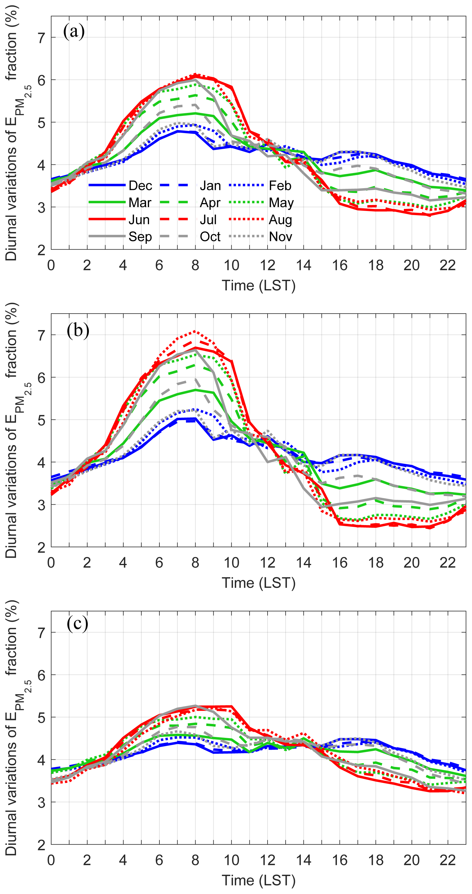
Figure 7The 5-year mean diurnal variations of dynamics-based PM2.5 emission fractions averaged over (a) mainland China, (b) megacities with an urban population ≥ 5 million, and (c) non-megacities with an urban population < 5 million.
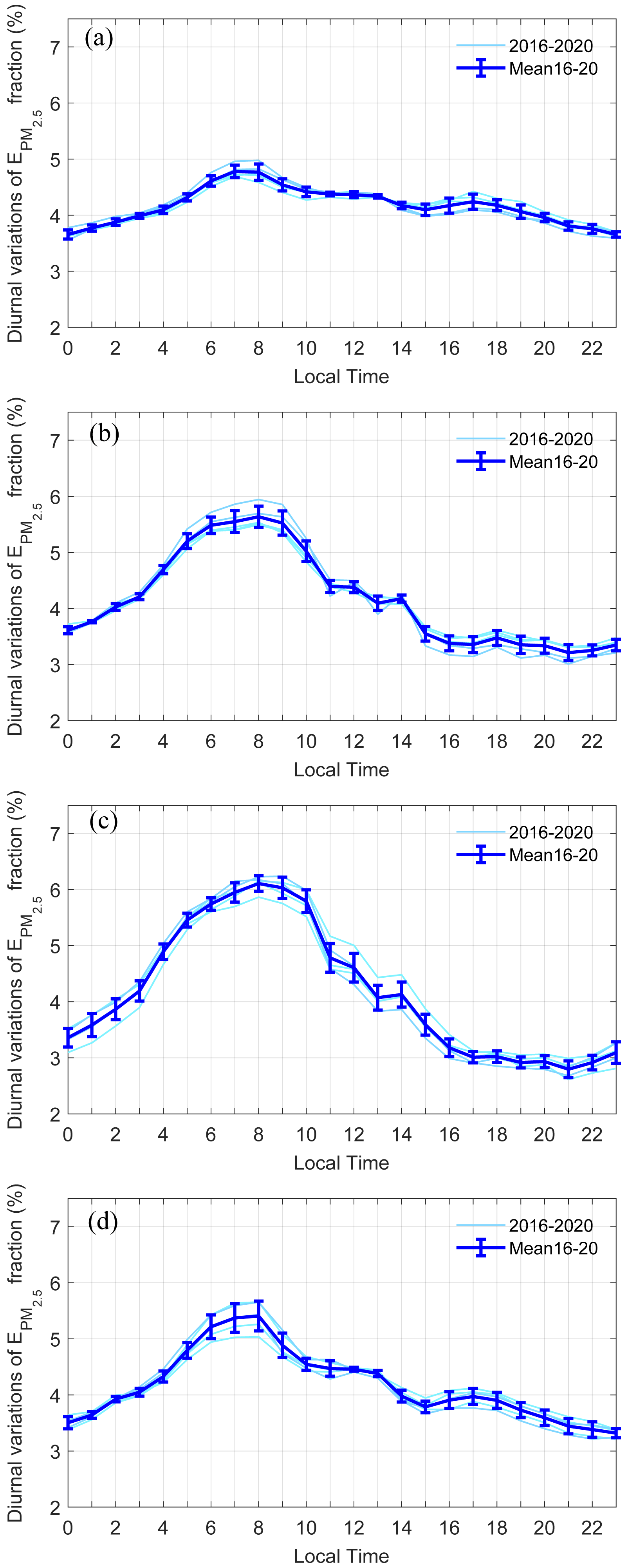
Figure 8Diurnal variations of dynamics-based PM2.5 emission fractions for the years 2016–2020 (light blue), and the 5-year mean fractions, with bars denoting 1 standard deviation of the 5-year variations (dark blue), are averaged over mainland China for (a) January, (b) April, (c) July, and (d) October.
The 5-year mean diurnal variations of the estimated PM2.5 emission fraction for mainland China show that, despite the monthly variations of PM2.5 emissions, the diurnal-variation fractions for November, December, January, and February are similar, while those for June, July, and August are similar (Fig. 7a). There are stronger diurnal variations of PM2.5 emissions in summer than in winter, which are represented by larger PM2.5 emission fractions during the morning and fewer PM2.5 emission fractions during evening. The diurnal variations of PM2.5 emissions from March to May gradually transform from the patterns of winter to those of summer and vice versa for the diurnal variations of PM2.5 emissions from September to November. The monthly changes in diurnal variations of PM2.5 emissions are consistent with the seasonal dependence since monthly variations of PM2.5 emissions are mainly related to the variations of residential consumptions (Li et al., 2017) in which the space heating has nearly no diurnal variations, and then larger PM2.5 emissions during winter lead to reduced diurnal variations compared to in summer. Similarly to the monthly fractions of estimated PM2.5 emissions for mainland China, diurnal variations of PM2.5 emission fractions are consistent across years for a given month (Fig. 8). Table 2 gives 5-year mean diurnal variations of the estimated PM2.5 emission fractions for each month. Based on these high-resolution diurnal-variation fractions, hourly estimates of PM2.5 emissions can be objectively obtained for a given monthly estimated PM2.5 emission.
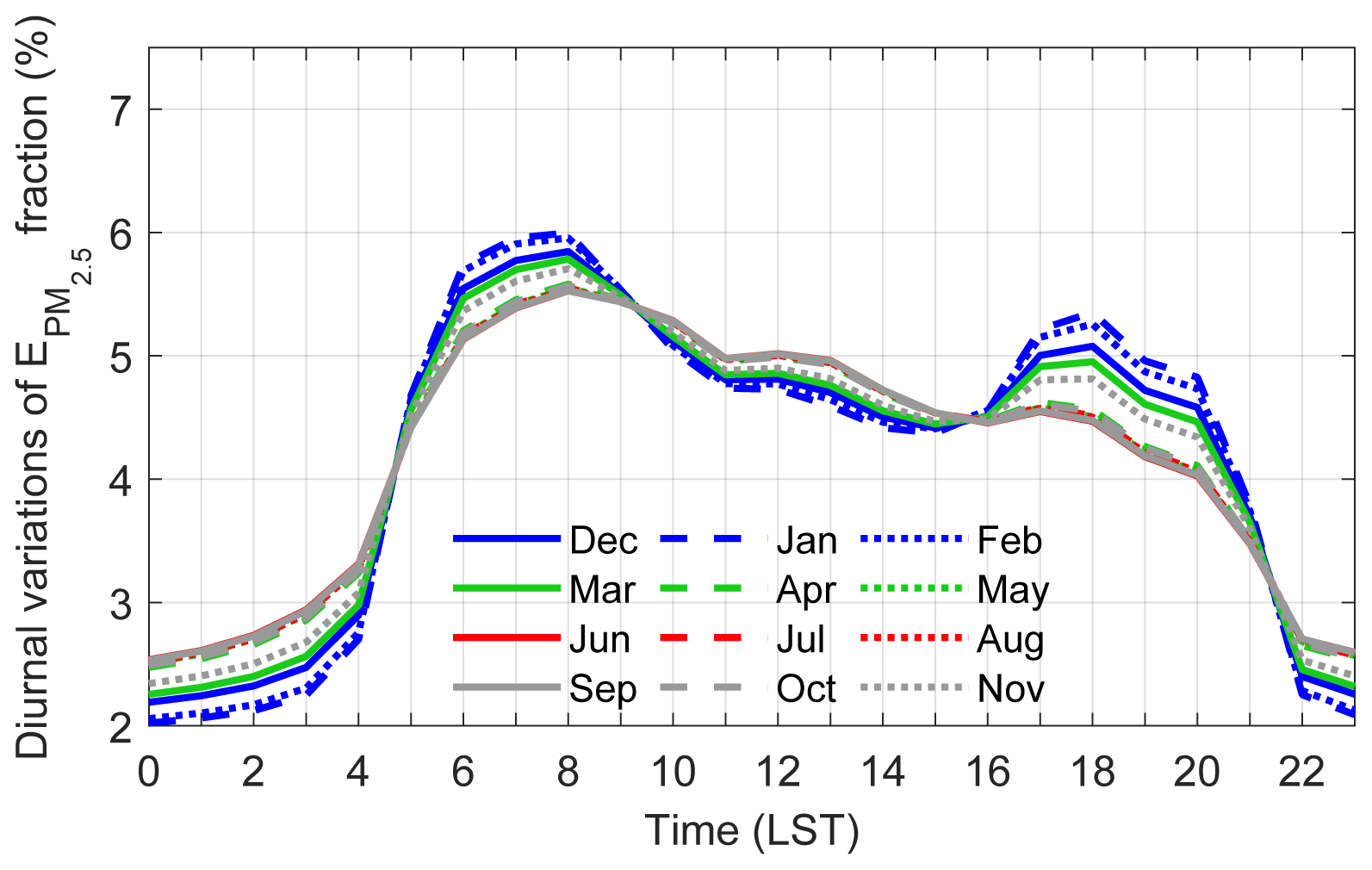
Figure 9Diurnal variations of PM2.5 emission fractions for each month based on diurnal variation profiles from the US and EU (Wang et al., 2010).
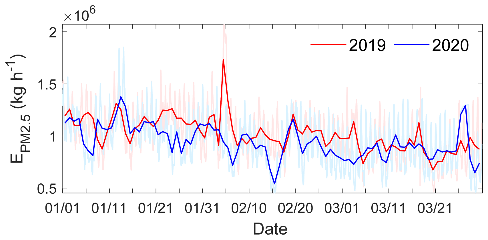
Figure 10Hourly (light red and blue) and daily (dark red and blue) dynamics-based PM2.5 emission estimates (kg h−1) summed over mainland China from January to March for the years 2019 and 2020.
Despite the high temporal resolution, the DEPE also has the ability to analyse diurnal variations for specific cities. The monthly changes in the diurnal variations of PM2.5 emissions estimated for megacities with urban populations larger than 5 million and non-megacities with urban populations smaller than 5 million (China State Council, 2013) are consistent with those estimated from mainland China (Fig. 7). Compared to the diurnal variations of PM2.5 emissions estimated for mainland China, the megacities have stronger diurnal variations, while the non-megacities have weaker diurnal variations. These detailed descriptions of PM2.5 emissions that are usually absent in common emission estimates can be essential for PM2.5 simulation, especially for providing timely and realistic guidance for severe haze events.
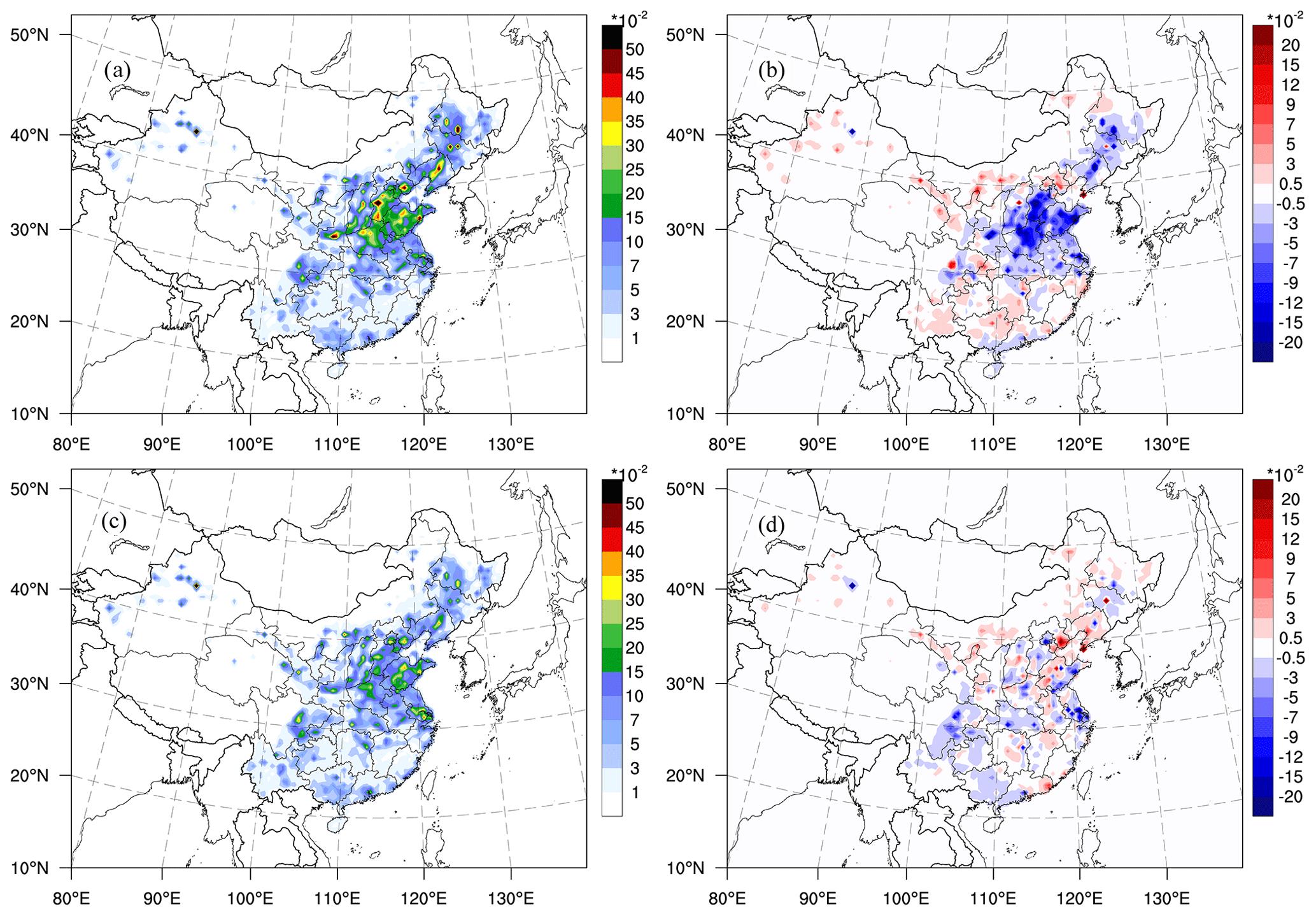
Figure 11Spatial distributions of dynamics-based PM2.5 emission estimates (µg m−2 s−1) in (a) February and (c) March of the year 2019 and spatial distributions of dynamics-based PM2.5 emission reductions of the year 2020 compared to the year 2019 for (b) February and (d) March.
There has been a lack of local measurements for diurnal variations and widely adopted diurnal variation profiles of PM2.5 emissions in China. Compared to the diurnal variations of PM2.5 emission fractions estimated based on diurnal variation profiles from the US and EU (Wang et al., 2010; Du et al., 2020), the estimated PM2.5 emission fractions are 1.25 % larger during the evening, which greatly changes the diurnal variations of DEPE. The noon and evening peaks estimated from DEPE have smaller PM2.5 emission fractions, with mean underestimations of PM2.5 emission fractions of 0.40 % and 0.83 % for noon peak and evening peak, respectively (Figs. 7a and 9). In fact, the smaller evening peaks of Wang et al. (2010) occurred in November, December, January, February, and March, while they are almost indistinct from April to October, similarly to those from DEPE. The morning peak of Wang et al. (2010) is similar to that of DEPE for spring and fall, but the former overestimates PM2.5 emission fractions by 0.57 % for winter, while it underestimates PM2.5 emission fractions by 1.05 % for summer. Due to the overestimated peaks, diurnal variations of Wang et al. (2010) have a sharper appearance rate for the morning peak and a disappearance rate for the evening peak. Compared to the diurnal variations based on diurnal variation profiles from the US and EU (Wang et al., 2010), the diurnal variations of the DEPE are constrained by the atmospheric–chemical model and observed PM2.5 concentrations, which can objectively determine the diurnal variations of PM2.5 emissions for specific regions and seasons.
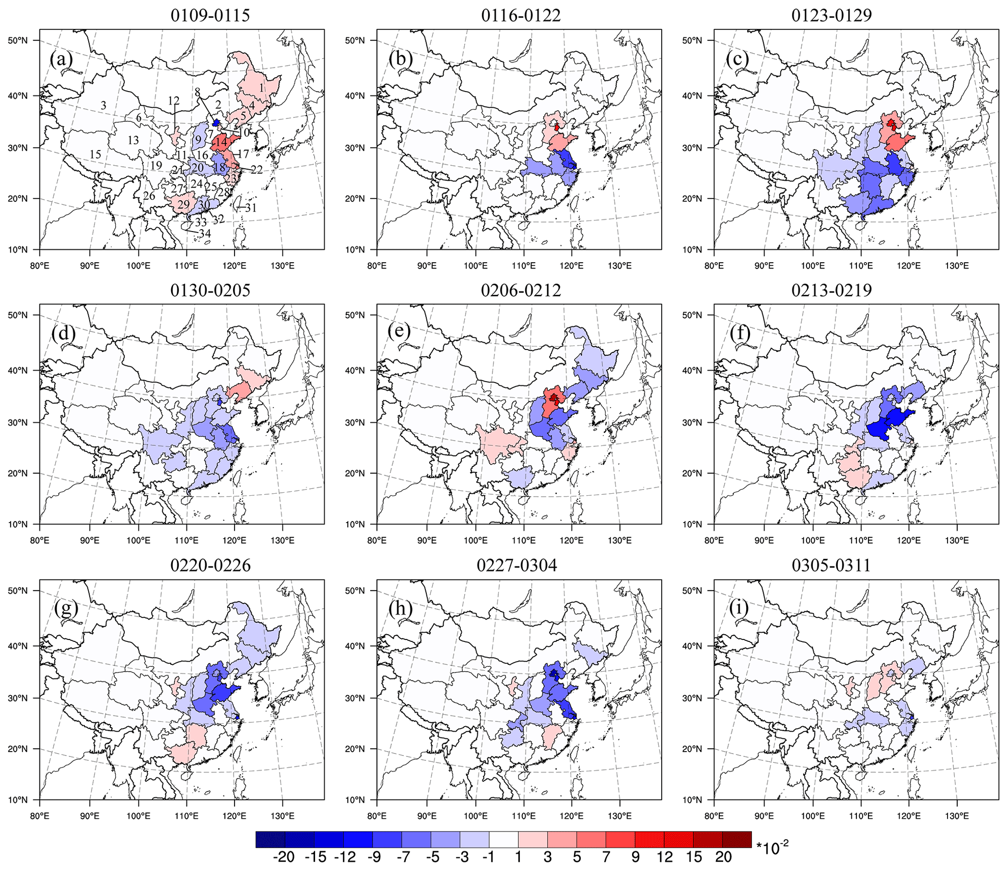
Figure 12Mean spatial distributions of PM2.5 emission differences (µg m−2 s−1) between the years 2020 and 2019 for 9 weeks starting on 9 January 2020. Negative (positive) values indicate that the PM2.5 emissions of the year 2020 are smaller (larger) than those of the year 2019. The numbers in (a) denote provinces as follows: (1) Heilongjiang, (2) Neimenggu, (3) Xinjiang, (4) Jilin, (5) Liaoning, (6) Gansu, (7) Hebei, (8) Beijing, (9) Shanxi, (10) Tianjin, (11) Shanxi, (12) Ningxia, (13) Qinghai, (14) Shandong, (15) Xizang, (16) Henan, (17) Jiangsu, (18) Anhui, (19) Sichuan, (20) Hubei, (21) Chongqing, (22) Shanghai, (23) Zhejiang, (24) Hunan, (25) Jiangxi, (26) Yunnan, (27) Guizhou, (28) Fujian, (29) Guangxi, (30) Guangdong, (31) Taiwan, (32) Hong Kong, (33) Macao, (34) Hainan.
The abrupt changes in PM2.5 emissions during the initial stage of COVID-19 in China provide a natural case study to validate the ability of the dynamic-based data assimilation method to obtain high-temporal-resolution PM2.5 emission estimates. The abrupt outbreak of the COVID-19 pandemic has produced dramatic socioeconomic impacts in China. To prevent the virus from spreading, a lockdown was first implemented on 23 January 2020 in Wuhan, Hubei Province, and subsequently, the national lockdown was enforced in China (Liu et al., 2020; Huang et al., 2020; Zhu et al., 2021). Consequently, the total PM2.5 emissions of February 2020 for China show an obvious decrease compared to those of previous years (Fig. 3). The high=temporal-resolution DEPE reveals the detailed changes of PM2.5 emissions with time (Fig. 10). The PM2.5 emissions started to decrease right around the COVID outbreak and had been smaller than those of the year 2019 till early March. The emissions in the following months of 2020 were similar to those of 2019 due to the epidemic prevention and control policies enforced by the Chinese government. During February 2020, the DEPE showed significant reductions at the North China Plain and northeast of China, where prominent PM2.5 emissions occurred, while spotted PM2.5 emission differences with small magnitudes were shown in the other regions (Fig. 11a–b). Along with recovery from COVID-19, the estimated PM2.5 emissions rebounded in March (Figs. 3a, 10, 11c–d), which is ascribed to the national work resumption. Thus, the DEPE is able to timeously reflect the dynamic response of PM2.5 emissions to COVID-19. Although similar emission reductions and emission trends are obtained from the bottom-up technique (Zheng et al., 2021), the reduction amount and ratio from the bottom-up technique are larger than those estimated from DEPE (Fig. 10 and Table 1). This is possibly due to significant reductions in PM2.5 emissions from the residential sector, as in the bottom-up technique (Zheng et al., 2021); however, PM2.5 emissions from the residential sector might not have significantly changed around the COVID outbreak.
To avoid fluctuations due to diurnal variations and monthly changes in PM2.5 emissions, 7 d averaged PM2.5 emission differences between the years 2020 and 2019 are used to analyse the dynamic impact of COVID-19 on PM2.5 emissions (Fig. 12). Before the lockdown, there were slight PM2.5 emission differences over several provinces (Fig. 12a–b). During the first week of lockdown, PM2.5 emission reductions larger than (µg m−2 s−1) – that is about 60 %–70 % emission reductions – occurred in the Hubei, Hunan, Guangdong, Anhui, and Zhejiang provinces (Fig. 12c). The PM2.5 emission reduction extended to BTH and the Shandong Province during the second week of lockdown (Fig. 12d) and continuously spread to the three northeast provinces of China during the third week of lockdown (Fig. 12e). During the third week of lockdown, the increased PM2.5 emissions for BTH and SCR were possibly caused by the long national vacation of the spring holiday of the year 2019 (Ji et al., 2018). The inhomogeneous spatial variations of PM2.5 emissions possibly relate to different traditions and policy enforcements for different provinces. The PM2.5 emission reduction had been maintained over the central and northern parts of China till early March when the lockdown was lifted (Fig. 12f–i). Though it is hard to see continuous and consistent signals of lockdown for the whole China, the timely DEPE can provide up-to-date guidance for quantifying the socioeconomic impacts of rare events with large emission changes such as the COVID-19 pandemic.
High-temporal-resolution and dynamics-based estimations of PM2.5 emissions can be objectively and optimally obtained by assimilating past and future observed surface PM2.5 concentrations through flow-dependent error statistics. This advanced assimilation strategy can be applied for emission estimates of other chemical species when corresponding observations are available and can extend to observation types besides the surface concentrations, like the aerosol optical depth (Liu et al., 2011; Choi et al., 2020). Moreover, current estimates of PM2.5 emissions are lacking in terms of explicit representations of primary and secondary PM2.5, which could be resolved by joint estimation of the source emissions and primary and secondary PM2.5 given the concentration observations. Another deficiency of this top-down technique is that it cannot directly determine dynamics-based PM2.5 emissions for different sectors and contributions from different policies, although the bottom-up technique has the potential to untangle the different contributions from different policies and quantify the different impacts on different sectors. However, this top-down technique can be integrated into the bottom-up technique to retain the advantages of both methods. One future work is to integrate the top-down technique with the bottom-up one, through which the emission estimates for different sectors and polices could be quantified. The annual emission estimates from the bottom-up technique can be further downscaled to hourly estimates by first distributing the annual amount to each month through the monthly allocations estimated from the top-down technique, then assuming evenly daily distribution and finally applying the fractions of diurnal variation estimated from the top-down technique. The information collected by the bottom-up technique is retained, while the common drawback of a coarse temporal resolution for the bottom-up technique is remedied. The integrated bottom-up and top-down techniques can improve spatiotemporal representations of source emissions across timescales and sectors, which is beneficial for emission inventories, air quality forecasts, regulation policies, and emission trading schemes.
The meteorological data used for meteorological initial conditions and boundary conditions are available from the University Corporation for Atmospheric Research (UCAR) Research Data Archive (https://rda.ucar.edu/datasets/ds083.3, NCEP, 2015). The assimilated meteorological observations are available from the UCAR Research Data Archive (https://rda.ucar.edu/datasets/ds337.0/, NCEP, 2008), and the assimilated chemical observations are available from https://aqicn.org/map/china/cn/ (last access: 6 November 2023). The prescribed time-invariant anthropogenic emissions are available from the Emission Database for Global Atmospheric Research for Hemispheric Transport of Air Pollution (EDGAR-HTAP) inventory (https://data.jrc.ec.europa.eu/dataset/jrc-edgar-htap_v2-2, Janssens-Maenhout et al., 2015a) and the Multi-resolution Emission Inventory (MEIC Team, 2018).
The WRF-Chem model version 3.6.1 is available from https://www2.mmm.ucar.edu/wrf/users/download/get_sources.html#WRF-Chem (WRF-Chem, 2014; Grell et al., 2005). The NOAA operational EnKF system is available from https://dtcenter.org/community-code/gridpoint-statistical-interpolation-gsi (Hu et al., 2018).
The supplement related to this article is available online at: https://doi.org/10.5194/acp-23-14505-2023-supplement.
ZMT and MZ designed the study, and ZP and LL prepared the assimilation algorithm, performed the numerical experiments, analysed the data assimilation results, and drafted the initial manuscript. ZMT, MZ, and AD contributed to the data interpretation. XK processed the hourly chemical observations. ZP, LL, ZMT, MZ, AD, and XK contributed to the discussion, writing, and editing of the manuscript.
The contact author has declared that none of the authors has any competing interests.
Publisher’s note: Copernicus Publications remains neutral with regard to jurisdictional claims made in the text, published maps, institutional affiliations, or any other geographical representation in this paper. While Copernicus Publications makes every effort to include appropriate place names, the final responsibility lies with the authors.
The authors are grateful to the three anonymous reviewers for their invaluable suggestions. We are grateful to the High-Performance Computing Center of Nanjing University for doing the cycling ensemble assimilation experiments.
This work was sponsored by the National Natural Science Foundation of China (grant nos. 42141017, 41922036, 42275153, and 41975004).
This paper was edited by Leiming Zhang and reviewed by three anonymous referees.
Attri, A. K., Kumar, U., and Jain, V. K.: Microclimate: formation of ozone by fireworks, Nature, 411, 1015, https://doi.org/10.1038/35082634, 2001.
Barker, D., Huang, X.-Y., Liu, Z., Auligné, T., Zhang, X., Rugg, S., Ajjaji, R., Bourgeois, A., Bray, J., Chen, Y., Demirtas, M., Guo, Y.-R., Henderson, T., Huang, W., Lin, H.-C., Michalakes, J., Rizvi, S., and Zhang, X.: The Weather Research and Forecasting Model's Community Variational/Ensemble Data Assimilation System: WRFDA, B. Am. Meteorol. Soc., 93, 831–843, https://doi.org/10.1175/BAMS-D-11-00167.1, 2012.
Cao, H., Fu, T.-M., Zhang, L., Henze, D. K., Miller, C. C., Lerot, C., Abad, G. G., De Smedt, I., Zhang, Q., van Roozendael, M., Hendrick, F., Chance, K., Li, J., Zheng, J., and Zhao, Y.: Adjoint inversion of Chinese non-methane volatile organic compound emissions using space-based observations of formaldehyde and glyoxal, Atmos. Chem. Phys., 18, 15017–15046, https://doi.org/10.5194/acp-18-15017-2018, 2018.
Chen, C., Dubovik, O., Henze, D. K., Chin, M., Lapyonok, T., Schuster, G. L., Ducos, F., Fuertes, D., Litvinov, P., Li, L., Lopatin, A., Hu, Q., and Torres, B.: Constraining global aerosol emissions using POLDER/PARASOL satellite remote sensing observations, Atmos. Chem. Phys., 19, 14585–14606, https://doi.org/10.5194/acp-19-14585-2019, 2019.
Chin, M., Rood, R. B., Lin, S. J., Muller, J. F., and Thompson, A. M.: Atmospheric sulfur cycle simulated in the global model GO-CART: Model description and global properties, J. Geophys. Res.-Atmos., 105, 24671–24687, 2000.
China State Council: Action Plan on Prevention and Control of Air Pollution, China State Council, Beijing, China, http://www.gov.cn/zwgk/2013-09/12/content_2486773.htm (last access: 6 November 2023), 2013.
Choi, Y., Chen, S. H., Huang, C. C., Earl, K., Chen, C. Y., Schwartz, C. S., and Matsui, T.: Evaluating the impact of assimilating aerosol optical depth observations on dust forecasts over North Africa and the East Atlantic using different data assimilation methods, J. Adv. Model. Earth Sy., 12, e2019MS001890, https://doi.org/10.1029/2019ms001890, 2020.
Du, Q., Zhao, C., Zhang, M., Dong, X., Chen, Y., Liu, Z., Hu, Z., Zhang, Q., Li, Y., Yuan, R., and Miao, S.: Modeling diurnal variation of surface PM2.5 concentrations over East China with WRF-Chem: impacts from boundary-layer mixing and anthropogenic emission, Atmos. Chem. Phys., 20, 2839–2863, https://doi.org/10.5194/acp-20-2839-2020, 2020.
Gaspari, G. and Cohn S. E.: Construction of correlation functions in two and three dimensions, Q. J. Roy. Meteorol. Soc., 125, 723–757, 1999.
Ginoux, P., Chin, M., Tegen, I., Prospero, J. M., Holben, B., Dubovik, O., and Lin, S.-J.: Sources and distributions of dust aerosols simulated with the GOCART model, J. Geophys. Res., 106, 20255–20273, https://doi.org/10.1029/2000JD000053, 2001.
Grell, G., Peckham, S. E., Schmitz, R., McKeen, S. A., Frost, G., Skamarock, W. C., and Eder, B.: Fully coupled “online” chemistry within the WRF model, Atmos. Environ., 39, 6957–6975, https://doi.org/10.1016/j.atmosenv.2005.04.027, 2005.
Guenther, A., Hewitt, C. N., Erickson, D., Fall, R., Geron, C., Graedel, T., Harley, P., Klinger, L., Lerdau, M., McKay, W., Pierce, T., Scholes, B., Steinbrecher, R., Tallamraju, R., Taylor, J., and Zimmerman, P.: A global model of natural volatile organic compound emissions, J. Geophys. Res., 100, 8873–8892, https://doi.org/10.1029/94JD02950, 1995.
Huang, J., Pan, X. C., Guo, X. B., and Li, G. X.: Health impact of China's Air Pollution Prevention and Control Action Plan: an analysis of national air quality monitoring and mortality data, Lancet Planet. Health, 2, E313–E323, https://doi.org/10.1016/S2542-5196(18)30141-4, 2018.
Huang, X., Ding, A., Gao, J., Zheng, B., Zhou, D., Qi, X., Tang, R., Wang, J., Ren, C., Nie, W., Chi, X., Xu, Z., Chen, L., Li, Y., Che, F., Pang, N., Wang, H., Tong, D., Qin, W., Cheng, W., Liu, W., Fu, Q., Liu, B., Chai, F., Davis, S. J., Zhang, Q., and He, K.: Enhanced secondary pollution offset reduction of primary emissions during COVID-19 lockdown in China, Nat. Sci. Rev., 8, nwaa137, https://doi.org/10.1093/nsr/nwaa137, 2020.
Hu, M., Ge, G., Zhou, C., Stark, D., Shao, H., Newman, K., Beck, J., and Zhang, X.: Grid-point Statistical Interpolation (GSI) User's Guide Version 3.7, Developmental Testbed Center [code], https://dtcenter.org/community-code/gridpoint-statistical-interpolation-gsi/documentation, GSI (V3.7)/EnKF (V1.3) System, https://dtcenter.org/community-code/gridpoint-statistical-interpolation-gsi (last access: 6 November 2023), 2018.
Janssens-Maenhout, G., Crippa, M., Guizzardi, D., Dentener, F., Muntean, M., Pouliot, G., Keating, T., Zhang, Q., Kurokawa, J., Wankmüller, R., Denier van der Gon, H., Kuenen, J. J. P., Klimont, Z., Frost, G., Darras, S., Koffi, B., and Li, M.: HTAP_v2.2, https://data.jrc.ec.europa.eu/dataset/jrc-edgar-htap_v2-2 (last access: 6 November 2023), 2015a.
Janssens-Maenhout, G., Crippa, M., Guizzardi, D., Dentener, F., Muntean, M., Pouliot, G., Keating, T., Zhang, Q., Kurokawa, J., Wankmüller, R., Denier van der Gon, H., Kuenen, J. J. P., Klimont, Z., Frost, G., Darras, S., Koffi, B., and Li, M.: HTAP_v2.2: a mosaic of regional and global emission grid maps for 2008 and 2010 to study hemispheric transport of air pollution, Atmos. Chem. Phys., 15, 11411–11432, https://doi.org/10.5194/acp-15-11411-2015, 2015b.
Ji, D., Cui, Y., Li, L., He, J., Wang, L., Zhang, H., Wang, W., Zhou, L., Maenhaut, W., Wen, T., and Wang, Y.: Characterization and source identification of fine particulate matter in urban Beijing during the 2015 Spring Festival, Sci. Total Environ., 628–629, 430–440, https://doi.org/10.1016/j.scitotenv.2018.01.304, 2018.
Jiang, Z., Worden, J. R., Worden, H., Deeter, M., Jones, D. B. A., Arellano, A. F., and Henze, D. K.: A 15-year record of CO emissions constrained by MOPITT CO observations, Atmos. Chem. Phys., 17, 4565–4583, https://doi.org/10.5194/acp-17-4565-2017, 2017.
Kalnay, E.: Atmospheric modeling, data assimilation and predictability, Cambridge: Cambridge University Press, p. 341, https://doi.org/10.1017/CBO9780511802270, 2002.
Kleist, D. T., Parrish, D. F., Derber, J. C., Treadon, R., Errico, R. M., and Yang, R.: Improving incremental balance in the GSI 3DVAR analysis system, Mon. Weather Rev., 137, 1046–1060, https://doi.org/10.1175/2008MWR2623.1, 2009.
Le, T., Wang, Y., Liu, L., Yang, J., Yung, Y. L., Li, G., and Seinfeld, J. H.: Unexpected air pollution with marked emission reductions during the COVID-19 outbreak in China, Science, 369, 702–706, https://https://doi.org/10.1126/science.abb7431, 2020.
Lei, Y., Zhang, Q., He, K. B., and Streets, D. G.: Primary anthropogenic aerosol emission trends for China, 1990–2005, Atmos. Chem. Phys., 11, 931–954, https://doi.org/10.5194/acp-11-931-2011, 2011.
Li, J. and Wang, Y.: Inferring the anthropogenic NOx emission trend over the United States during 2003–2017 from satellite observations: was there a flattening of the emission trend after the Great Recession?, Atmos. Chem. Phys., 19, 15339–15352, https://doi.org/10.5194/acp-19-15339-2019, 2019.
Li, K., Jacob, D. J., Liao, H., Zhu, J., Shah, V., Shen, L., Bates, K. H., Zhang, Q., and Zhai, S.: A Two-Pollutant Strategy for Improving Ozone and Particulate Air Quality in China, Nat. Geosci., 12, 906–910, https://doi.org/10.1038/s41561-019-0464-x, 2019.
Li, N., Tang, K., Wang, Y., Wang, J., Feng, W., Zhang, H., Liao, H., Hu, J., Long, X., and Shi, C.: Is the efficacy of satellite-based inversion of SO2 emission model dependent?, Environ. Res. Lett., 16, 035018, https://doi.org/10.1088/1748-9326/abe829, 2021.
Li, M., Zhang, Q., Streets, D. G., He, K. B., Cheng, Y. F., Emmons, L. K., Huo, H., Kang, S. C., Lu, Z., Shao, M., Su, H., Yu, X., and Zhang, Y.: Mapping Asian anthropogenic emissions of non-methane volatile organic compounds to multiple chemical mechanisms, Atmos. Chem. Phys., 14, 5617–5638, https://doi.org/10.5194/acp-14-5617-2014, 2014.
Li, M., Zhang, Q., Kurokawa, J.-I., Woo, J.-H., He, K., Lu, Z., Ohara, T., Song, Y., Streets, D. G., Carmichael, G. R., Cheng, Y., Hong, C., Huo, H., Jiang, X., Kang, S., Liu, F., Su, H., and Zheng, B.: MIX: a mosaic Asian anthropogenic emission inventory under the international collaboration framework of the MICS-Asia and HTAP, Atmos. Chem. Phys., 17, 935–963, https://doi.org/10.5194/acp-17-935-2017, 2017.
Liu, J., Yin, H., Tang, X., Zhu, T., Zhang, Q., Liu, Z., Tang, X., and Yi, H.: Transition in air pollution, disease burden and health cost in China: A comparative study of long-term and short-term exposure, Environ. Pollut., 277, 116770, https://doi.org/10.1016/j.envpol.2021.116770, 2021.
Liu, T., Cai, Y., Feng, B., Cao, G., Lin, H., Xiao, J., Li, X., Liu, S., Pei, L., Fu, L., Yang, X., and Zhang, B.: Long-term mortality benefits of air quality improvement during the twelfth five-year-plan period in 31 provincial capital cities of China, Atmos. Environ., 173, 53–61, https://doi.org/10.1016/j.atmosenv.2017.10.054, 2018.
Liu, T., Wang, X. Y., Hu, J. L., Wang, Q., An, J. Y., Gong, K. J., Sun, J. J., Li, L., Qin, M. M., Li, J. Y., Tian, J. J., Huang, Y. W., Liao, H., Zhou, M., Hu, Q. Y., Yan, R. S., Wang, H. L., and Huang, C.: Driving Forces of Changes in Air Quality during the COVID-19 Lockdown Period in the Yangtze River Delta Region, China, Environ. Sci. Technol., 7, 779–786, https://doi.org/10.1021/acs.estlett.0c00511, 2020.
Liu, Z., Liu, Q., Lin, H. C., Schwartz, C. S., Lee, Y. H., and Wang, T.: Three-dimensional variational assimilation of MODIS aerosol optical depth: implementation and application to a dust storm over East Asia, J. Geophys. Res., 116, D23206, https://doi.org/10.1029/2011JD016159, 2011.
MEIC Team: The Multi-resolution Emission Inventory Model for Climate and Air Pollution Research, MEIC Model [data], http://www.meicmodel.org/ (last access: 6 November 2023), 2018.
Miyazaki, K., Eskes, H., Sudo, K., Boersma, K. F., Bowman, K., and Kanaya, Y.: Decadal changes in global surface NOx emissions from multi-constituent satellite data assimilation, Atmos. Chem. Phys., 17, 807–837, https://doi.org/10.5194/acp-17-807-2017, 2017.
Miyazaki, K., Bowman, K., Sekiya, T., Eskes, H., Boersma, F., Worden, H., Livesey, N., Payne, V. H., Sudo, K., Kanaya, Y., Takigawa, M., and Ogochi, K.: Updated tropospheric chemistry reanalysis and emission estimates, TCR-2, for 2005–2018, Earth Syst. Sci. Data, 12, 2223–2259, https://doi.org/10.5194/essd-12-2223-2020, 2020.
Müller, J.-F., Stavrakou, T., Bauwens, M., George, M., Hurtmans, D., Coheur, P.-F., Clerbaux, C., and Sweeney, C.: Top-Down CO Emissions Based on IASI Observations and Hemispheric Constraints on OH Levels, Geophys. Res. Lett., 45, 1621–1629, https://doi.org/10.1002/2017GL076697, 2018.
NCEP: National Centers for Environmental Prediction/National Weather Service/NOAA/U.S. Department of Commerce, updated daily.NCEP ADP Global Upper Air and Surface Weather Observations (PREPBUFR format). Research Data Archive at the National Center for Atmospheric Research, Computational and Information Systems Laboratory [data], https://doi.org/10.5065/Z83F-N512, 2008.
NCEP: National Centers for Environmental Prediction/National Weather Service/NOAA/U.S. Department of Commerce, updated daily. NCEP GDAS/FNL 0.25 Degree Global Tropospheric Analyses and Forecast Grids. Research Data Archive at the National Center for Atmospheric Research, Computational and Information Systems Laboratory [data], https://doi.org/10.5065/D65Q4T4Z, 2015.
Peng, Z., Zhang, M., Kou, X., Tian, X., and Ma, X.: A regional carbon data assimilation system and its preliminary evaluation in East Asia, Atmos. Chem. Phys., 15, 1087–1104, https://doi.org/10.5194/acp-15-1087-2015, 2015.
Peng, Z., Liu, Z., Chen, D., and Ban, J.: Improving PM2.5 forecast over China by the joint adjustment of initial conditions and source emissions with an ensemble Kalman filter, Atmos. Chem. Phys., 17, 4837–4855, https://doi.org/10.5194/acp-17-4837-2017, 2017.
Peng, Z., Lei, L., Liu, Z., Sun, J., Ding, A., Ban, J., Chen, D., Kou, X., and Chu, K.: The impact of multi-species surface chemical observation assimilation on air quality forecasts in China, Atmos. Chem. Phys., 18, 17387–17404, https://doi.org/10.5194/acp-18-17387-2018, 2018.
Peng, Z., Lei, L., Liu, Z., Liu, H., Chu, K., and Kou, X.: Impact of Assimilating Meteorological Observations on Source Emissions Estimate and Chemical Simulations, Geophys. Res. Lett., 47, e2020GL089030, https://doi.org/10.1029/2020GL089030, 2020.
Peters, W., Jacobson, A. R., Sweeney, C., Andrews, A. E., Conway, T. J., Masarie, K., Miller, J. B., Bruhwiler, L. M. P., Petron, G., Hirsch, A. I.,Worthy, D. E. J., van derWerf, G. R., Randerson, J. T.,Wennberg, P. O., Krol, M. C., and Tans, P. P.: An atmospheric perspective on North American carbon dioxide exchange: CarbonTracker, P. Natl. Acad. Sci. USA, 104, 18925–18930, 2007.
Qu, Z., Henze, D. K., Capps, S. L., Wang, Y., Xu, X., and Wang, J.: Monthly top-down NOx emissions for China (2005–2012): a hybrid inversion method and trend analysis, J. Geophys. Res., 122, 4600–4625, https://doi.org/10.1002/2016JD025852, 2017.
Streets, D. G., Bond, T. M. L., Carmichael, G. R., Fernandes, S., Fu, Q., He, D., Klimont, Z., Nelson, S. M., Tsai, N. Y., Wang, M. Q., Woo, J.-H., and Yarber, K. F.: An inventory of gaseous and primary aerosol emissions in Asia in the year 2000, J. Geophys. Res., 108, 8809, https://doi.org/10.1029/2002JD003093, 2003.
Torn, R. D., Hakim, G. J., and Snyder, C.: Boundary conditions for limited-area ensemble Kalman filters, Mon. Weather Rev., 134, 2490–2502, 2006.
Wang, G., Cheng, S. Y., Wei, W., Yang, X. W., Wang, X. Q. Jia, J., Lang, J. L., and Lv, Z.: Characteristics and emission reduction measures evaluation of PM2.5 during the two major events: APEC and Parade, Sci. Total Environ., 595, 81–92, https://doi.org/10.1016/j.scitotenv.2017.03.231, 2017.
Wang, H., He, X., Liang, X., Choma, E. F., Liu, Y., Shan, L., Zheng, H., Zhang, S., Nielsen, C. P., Wang, S., Wu, Y., and Evans, J. S.: Health benefits of on-road transportation pollution control programs in China, P. Natl. Acad. Sci. USA, 117, 25370, https://doi.org/10.1073/pnas.1921271117, 2020.
Wang, X. Y., Liang, X. Z., Jiang, W. M., Tao, Z. N., Wang, J. X. L., Liu, H. N., Han, Z. W., Liu, S. Y., Zhang, Y. Y., Grell, G. A., and Peckham, S. E.: WRF-Chem simulation of East Asian air quality: Sensitivity to temporal and vertical emissions distributions, Atmos. Environ., 44, 660–669, 2010.
Wang, Z., Li, J., Wang, Z., Yang, W., Tang, X., Ge, B., Yan, P., Zhu, L., Chen, X., and Chen, H.: Modeling study of regional severe hazes over mid-eastern China in January 2013 and its implica- tions on pollution prevention and control, Sci. China Earth Sci., 57, 3–13, 2014.
Whitaker, J. S. and Hamill, T. M.: Ensemble data assimilation without perturbed observations, Mon. Weather Rev., 130, 1913–1924, 2002.
Whitaker, J. S. and Hamill, T. M.: Evaluating methods to account for system errors in ensemble data assimilation, Mon. Weather Rev., 140, 3078–3089, 2012.
WRF-Chem: version 3.6.1, WRF [code], https://www2.mmm.ucar.edu/wrf/users/download/get_sources.html#WRF-Chem (last access: 6 November 2023), 2014.
Yang, Y., Ren, L., Li, H., Wang, H., Wang, P., Chen, L., Yue, X., and Liao, H.: Fast climate responses to aerosol emission reductions during the COVID-19 pandemic, Geophys. Res. Lett., 47, e2020GL089788, https://doi.org/10.1029/2020gl089788, 2020.
Yin, L., Du, P., Zhang, M., Liu, M., Xu, T., and Song, Y.: Estimation of emissions from biomass burning in China (2003–2017) based on MODIS fire radiative energy data, Biogeosciences, 16, 1629–1640, https://doi.org/10.5194/bg-16-1629-2019, 2019.
Zhai, S., Jacob, D. J., Wang, X., Liu, Z., Wen, T., Shah, V., Li, K., Moch, J. M., Bates, K. H., Song, S., Shen, L., Zhang, Y., Luo, G., Yu, F., Sun, Y., Wang, L., Qi, M., Tao, J., Gui, K., Xu, H., Zhang, Q., Zhao, T., Wang, Y., Lee, H. C., Choi, H., and Liao, H.: Control of particulate nitrate air pollution in China, Nat. Geosci., 14, 1–7, 2021.
Zhang, L., Shao, J. Y., Lu, X., Zhao, Y. H., Hu, Y. Y., Henze, D. K., Liao, H., Gong, S., and Zhang, Q.: Sources and processes affect- ing fine particulate matter pollution over North China: An adjoint analysis of the Beijing APEC period, Environ. Sci. Technol., 50, 8731–8740, https://doi.org/10.1021/acs.est.6b03010, 2016.
Zhang, Q., Streets, D. G., Carmichael, G. R., He, K. B., Huo, H., Kannari, A., Klimont, Z., Park, I. S., Reddy, S., Fu, J. S., Chen, D., Duan, L., Lei, Y., Wang, L. T., and Yao, Z. L.: Asian emissions in 2006 for the NASA INTEX-B mission, Atmos. Chem. Phys., 9, 5131–5153, https://doi.org/10.5194/acp-9-5131-2009, 2009.
Zhang, Q., Zheng, Y., Tong, D., Shao, M., Wang, S., Zhang, Y., Xu, X., Wang, J., He, H., Liu, W., Ding, Y., Lei, Y., Li, J., Wang, Z., Zhang, X., Wang, Y., Cheng, J., Liu, Y., Shi, Q., Yan, L., Geng, G., Hong, C., Li, M., Liu, F., Zheng, B., Cao, J., Ding, A., Gao, J., Fu, Q., Huo, J., Liu, B., Liu, Z., Yang, F., He, K., and Hao, J.: Drivers of Improved PM2.5 Air Quality in China from 2013 to 2017, P. Natl. Acad. Sci. USA, 116, 24463–24469, https://doi.org/10.1073/pnas.1907956116, 2019.
Zheng, B., Tong, D., Li, M., Liu, F., Hong, C., Geng, G., Li, H., Li, X., Peng, L., Qi, J., Yan, L., Zhang, Y., Zhao, H., Zheng, Y., He, K., and Zhang, Q.: Trends in China's anthropogenic emissions since 2010 as the consequence of clean air actions, Atmos. Chem. Phys., 18, 14095–14111, https://doi.org/10.5194/acp-18-14095-2018, 2018.
Zheng, B., Geng, G., Ciais, P., Davis, S. J., Martin, R. V., Meng, J., Wu, N., Chevallier, F., Broquet, G., Boersma, F., van der A, R., Lin, J., Guan, D., Lei, Y., He, K., and Zhang, Q.: Satellite-based estimates of decline and rebound in China's CO2 emissions during COVID-19 pandemic, Sci. Adv., 6, eabd4998, https://doi.org/10.1126/sciadv.abd4998, 2020.
Zheng, B., Zhang, Q., Geng, G., Chen, C., Shi, Q., Cui, M., Lei, Y., and He, K.: Changes in China's anthropogenic emissions and air quality during the COVID-19 pandemic in 2020, Earth Syst. Sci. Data, 13, 2895–2907, https://doi.org/10.5194/essd-13-2895-2021, 2021.
Zhu, J., Chen, L., Liao, H., Yang, H., Yang, Y., and Yue, X.: Enhanced PM2.5 Decreases and O3 Increases in China during COVID-19 Lockdown by Aerosol-Radiation Feedback, Geophys. Res. Lett., 48, e2020GL090260, https://doi.org/10.1029/2020GL090260, 2021.
- Abstract
- Introduction
- Data assimilation and experimental design
- PM2.5 emission for years 2016–2020
- Diurnal variations of PM2.5 emissions
- Impact of COVID-19 on PM2.5 emissions
- Discussion
- Data availability
- Author contributions
- Competing interests
- Disclaimer
- Acknowledgements
- Financial support
- Review statement
- References
- Supplement