Assimilation of 3D polarimetric microphysical retrievals in a convective-scale NWP system

This study assimilates for the first time polarimetric C-band radar observations from the German meteorological service (DWD) into DWD's convective-scale model ICON-D2 using DWD's ensemble-based KENDA assimilation framework. We compare the assimilation of conventional observations (CNV) with the additional assimilation of radar reflectivity Z (CNV + Z), with the additional assimilation of liquid or ice water content (LWC or IWC) estimates below or above the melting layer instead of Z where available (CNV + LWC$/Z$ or CNV + IWC$/Z$ respectively). Hourly quantitative precipitation forecasts (QPF) are evaluated for two stratiform and one convective rainfall events in the summers of 2017 and 2021.

With optimized data assimilation settings (e.g., observation errors), the assimilation of LWC mostly improves first-guess QPF compared with the assimilation of Z alone (CNV + Z), whereas the assimilation of IWC does not, especially for convective cases, probably because of the lower quality of the IWC retrieval in these situations. Improvements are, however, notable for stratiform rainfall in 2021, for which the IWC estimator profits from better specific differential phase estimates owing to a higher radial radar resolution than the other cases. The assimilation of all radar data sets together (CNV + LWC + IWC + Z) yields the best first guesses.

All assimilation configurations with radar information consistently improve deterministic 9 h QPF compared with the assimilation of only conventional data (CNV). Forecasts based on the assimilation of LWC and IWC retrievals on average slightly improve Fraction Skill Score (FSS) and Frequency Bias (FBI) compared with the assimilation of Z alone (CNV + Z), especially when LWC is assimilated for the 2017 convective case and when IWC is assimilated for the high-resolution 2021 stratiform case. However, IWC assimilation again degrades forecast FSS for the convective cases. Forecasts initiated using all radar data sets together (CNV + LWC + IWC + Z) yield the best FSS. The development of IWC retrievals that are more adequate for convection constitutes one next step to further improving the exploitation of ice microphysical retrievals for radar data assimilation.

1 Introduction

Heavy precipitation events can pose serious risks to the public and have increased in frequency and strength since the middle of the 20th century (IPCC, 2021). Thus, improving quantitative precipitation forecasts (QPF) is and remains of high societal interest. With the ever-increasing computing power of meteorological forecasting centers, the resolution of operational numerical weather prediction (NWP) models has increased up to the convective scale, allowing more accurate QPF. NWP requires model states close to the true atmospheric state (model initialization), which is usually achieved by combining short-term model forecasts (first guesses) and observational data statistically, taking into account their respective uncertainties, a process known as data assimilation (DA; e.g., Talagrand, 1997). Proper initialization at convective scales is challenging, because uncertainties in convective processes are difficult to estimate, and because of the observations required to resolve moist convective processes. Weather surveillance radars can provide such data with unique temporal and spatial resolution, and have become an indispensable data source for convective-scale NWP over the past few decades.

Radar observations have been successfully assimilated into convective-scale NWP models, e.g., with 4D variational (4DVar; e.g., Lewis and Derber, 1985; Le Dimet and Talagrand, 1986) and 3D variational (3DVar; Courtier et al., 1998) DA methods (e.g., Sun and Crook, 1997, 1998; Xiao et al., 2005). Over the past two decades, radar DA using the ensemble Kalman filter (EnKF; Evensen, 1994), a Monte Carlo approximation of the original Kalman filter (Kalman, 1960), has become increasingly popular, particularly because of its ability to estimate the flow-dependent forecast uncertainty (the background error covariance matrix) at the convective-scale through an ensemble of model forecasts (e.g., Snyder and Zhang, 2003; Tong and Xue, 2005; Aksoy et al., 2009; Dowell et al., 2011; Tanamachi et al., 2013; Wheatley et al., 2015; Bick et al., 2016; Gastaldo et al., 2021). However, running a forecast ensemble of sufficient size to robustly estimate the forecast error covariance matrix is not feasible in operational routines owing to the connected high computational costs, which can lead to sampling errors that can cause filter divergence and spurious long-range correlations in the model domain (e.g., Houtekamer and Mitchell, 1998; Hamill et al., 2001). Observation localization (Ott et al., 2004), which limits the radius within which observations affect the analysis, is a common approach to mitigating this problem. The Local Ensemble Transform Kalman Filter (LETKF; Hunt et al., 2007), a manifestation of the EnKF in which observation localization is a key feature and which computes analyses at each grid point independently allowing for easy parallelization, is currently very popular in the DA community. In addition to being used for research purposes at the Japan Meteorological Agency (e.g., Miyoshi et al., 2010) and the European Centre for Medium-Range Weather Forecasts (e.g., Hamrud et al., 2015), the LETKF has been implemented operationally at the Italian Operational Centre for Meteorology (Gastaldo et al., 2021) as well as at the German Meteorological Service (Deutscher Wetterdienst, DWD), and MeteoSwiss. Assimilation of 3D radar observations with the LETKF has shown positive effects on short-term QPF (e.g., Bick et al., 2016; Gastaldo et al., 2021); at DWD, 3D radar DA with the LETKF became operational for the convective-scale NWP model ICON-D2 (limited area setup of the Icosahedral Nonhydrostatic model over Germany; Zängl et al., 2015) in spring 2021.

Radar DA has mainly focused on the horizontal radar reflectivity factor (hereafter simply reflectivity) Z and the radial velocity V, with only Z providing direct information on cloud and precipitation microphysical processes. Dual-polarization (i.e., linear orthogonal polarization diversity; Seliga and Bringi, 1976, 1978; hereafter referred to as polarimetric) radar observations provide additional information on clouds and precipitation, such as the size, shape, orientation, and composition of hydrometeors (e.g., Zrnic and Ryzhkov, 1999). Therefore, polarimetric radar observations can help to improve the representation of cloud-precipitation microphysics in NWP models, weather analyses, and consequently short-term QPF through model evaluation, parameterization developments, and DA (e.g., Kumjian, 2013; Zhang et al., 2019). Polarimetric radar observations have already been used to improve attenuation correction (e.g., Bringi et al., 1990; Testud et al., 2000; Snyder et al., 2010), quantitative precipitation estimation (e.g., Zrnic and Ryzhkov, 1996; Ryzhkov et al., 2005a; Tabary et al., 2011; Chen et al., 2021), severe weather observation and detection (e.g., Ryzhkov et al., 2005b; Bodine et al., 2013), hydrometeor classification (e.g., Park et al., 2009), and model evaluation (e.g., Jung et al., 2012; Putnam et al., 2014, 2017). However, exploitation of polarimetric information in DA is still in its infancy. One reason is the remaining uncertainties in the relationships between polarimetric radar moments and model microphysical state variables. Another reason is the lack of widespread operational polarimetric radar observations from national surveillance radar networks in the past. In recent years, many of these networks have been upgraded to polarimetry, e.g., in Germany, the USA, Canada, the UK, and China, providing a valuable new source of observational data for future operational NWP.

Polarimetric moments can be linked to microphysical model state variables using either radar forward operators or retrieval algorithms. Radar forward operators compute synthetic radar moments based, for example, on simulated parameterized particle size distributions, whereas retrievals estimate microphysical model state variables from radar observations prior to DA. The direct approach via forward operators is challenging because, for example, hydrometeor shape, size, and orientation distributions, all of which affect (polarimetric) radar observations, are still rather rudimentarily represented or rarely taken into account in NWP models (e.g., Schinagl et al., 2019). The indirect approach via retrievals circumvents these model deficiencies, but suffers from retrieval uncertainties. A few case studies from the USA, Japan, and China have already attempted the direct DA of polarimetric observations with some success using the EnKF (e.g., Jung et al., 2008, 2010; Putnam et al., 2019, 2021; Zhu et al., 2020) or the 3DVar method (e.g., Li et al., 2017; Du et al., 2021). Other studies have assimilated polarimetric observations indirectly via retrieved hydrometeor mixing ratios using the 4DVar approach (e.g., Wu et al., 2000), the 3DVar method (e.g., Li and Mecikalski, 2010, 2012), or the EnKF method (e.g., Yokota et al., 2016). Polarimetric data have also been used to modify cloud analysis schemes based on polarimetric signatures in storms (Carlin et al., 2017) or to improve hydrometeor classifications (Ding et al., 2022). To our knowledge, no study has yet assimilated polarimetric radar data in Central Europe. In preparation for the direct assimilation of polarimetric data, the single-polarization radar forward operator EMVORADO (Efficient Modular VOlume scan RADar Operator; Zeng et al., 2016), used operationally at DWD for the ICON-D2 model, is currently being upgraded to polarimetric capabilities, but is still in a testing phase. Regarding indirect assimilation, polarimetric retrieval algorithms for liquid and ice water content (LWC and IWC) have been proposed in the literature (e.g., Ryzhkov et al., 1998; Bringi and Chandrasekar, 2001; Doviak and Zrnic, 2006; Carlin et al., 2016, 2021; Ryzhkov and Zrnic, 2019; Bukovcic et al., 2020), but most of these algorithms were developed with a focus on S-band radars in the USA. The applicability of these retrieval relations for Germany with its C-band radar network and its quite different precipitation climatology may thus be limited. Recently, a hybrid polarimetric LWC estimator adapted to the German national C-band network has been developed by Reimann et al. (2021).

The present paper takes a first step toward the indirect assimilation of polarimetric radar observations using microphysical retrievals of LWC and IWC in Germany and evaluates their impact on short-term QPF relative to the direct assimilation of Z observations. Polarimetric radar observations from the German national C-band weather radar network are assimilated into the DWD ICON-D2 model using the corresponding DA framework KENDA (Kilometer-scale Ensemble Data Assimilation; Schraff et al., 2016) implementing the LETKF scheme. LWC and IWC data are estimated from the polarimetric measurements below and above the melting layer using the hybrid retrievals of Reimann et al. (2021) and Carlin et al. (2021) respectively. We attempt to identify suitable assimilation configurations for LWC and IWC based on first-guess QPF quality and provide first insights into how the indirect assimilation of polarimetric information affects short-term QPF up to a 9 h lead time. The study focuses on three intense precipitation periods in the summers of 2017 and 2021 over Germany.

The remainder of the paper is structured as follows. Section 2 briefly introduces the ICON-D2 model and the KENDA DA framework. Section 3 describes the data used and the applied microphysical retrieval algorithms. Section 4 shows the experimental setup including the technique of assimilating the LWC and IWC retrievals and the experiment parts. Section 5 presents the results of the experiments, and Sect. 6 presents the conclusions.

2 Forecast model and assimilation framework

2.1 The ICON-D2 model

The ICON (Icosahedral Nonhydrostatic) modeling framework (Zängl et al., 2015) is a global NWP and climate modeling system jointly developed by DWD and the Max Planck Institute for Meteorology in Hamburg, Germany, and became operational in DWD's forecasting system in 2015. In this study, we perform integrations with the convection-resolving, area-limited setup of the ICON model, ICON-D2, covering Germany and parts of its neighboring states. The ICON-D2 model uses an unstructured triangular grid with a resolution of about 2.2 km horizontally and 65 vertical levels; the near-ground levels are terrain-following and the higher levels gradually shift to constant heights toward the model top. Lateral boundary conditions are provided by simulations of the ICON-EU model, a nesting setup of the global ICON model over Europe. The ICON-D2 model became operational at DWD recently, ousting the previously used COSMO (COnsortium for Small-scale MOdeling) model (Baldauf et al., 2011).

The ICON-D2 model provides prognostic variables including the 3D wind velocity components and the virtual potential temperature. The total density of the air–water mixture and the individual mass fractions of dry air, water vapor, cloud water, cloud ice, rain, snow, and graupel are further prognostic variables, simulated in our study with the single-moment microphysics scheme (Doms et al., 2011), representing a two-component system of dry air and water, which can occur in all three states of matter.

2.2 The KENDA framework

The KENDA system, originally developed for the COSMO model, is now operationally used for the ICON-D2 model at DWD and includes the LETKF scheme (Hunt et al., 2007). KENDA employs one deterministic model run in addition to the current 40-member ensemble (40 + 1-mode), which is updated in the analysis using the Kalman gain for the ensemble mean K as

$$\begin{array}{}\text{(1)}& {\mathit{x}}^{\mathrm{a},\det }={\mathit{x}}^{\mathrm{b},\det }+\mathbf{K}\left({\mathit{y}}^{\mathrm{o}}-H\left({\mathit{x}}^{\mathrm{b},\det }\right)\right),\end{array}$$

with x^a,det and x^b,det the deterministic analysis and background, y^o the observation vector, and H a (nonlinear) observation operator (Schraff et al., 2016). KENDA comprises various tools beneficial for ensemble-based DA. Among them are horizontal and vertical observation localization with a Gaspari–Cohn correlation function (Gaspari and Cohn, 1999) using individual length-scales to scale the inverse observation error covariance matrix. Moreover, KENDA allows for analysis calculations on a coarsened grid (Yang et al., 2009) to reduce the computational costs in the analysis step. KENDA also includes, for example, multiplicative covariance inflation (Anderson and Anderson, 1999), relaxation to prior perturbations (Zhang et al., 2004), and relaxation to prior spread (Whitaker and Hamill, 2012).

The indirect assimilation of Z observations started at DWD in 2007 with Latent Heat Nudging (LHN; Stephan et al., 2008; Milan et al., 2008), which modifies the thermodynamic model state during model forward integration using low-elevation Z observations. LHN is applicable to both the ensemble and the deterministic run in KENDA. Recently, the direct assimilation of 3D Z and V observations from the German C-band radar network (see Fig. 1) in combination with LHN became operational in the ICON-D2 routine at DWD. Note that LHN and the assimilation of 3D V observations are not applied in this study (see below).

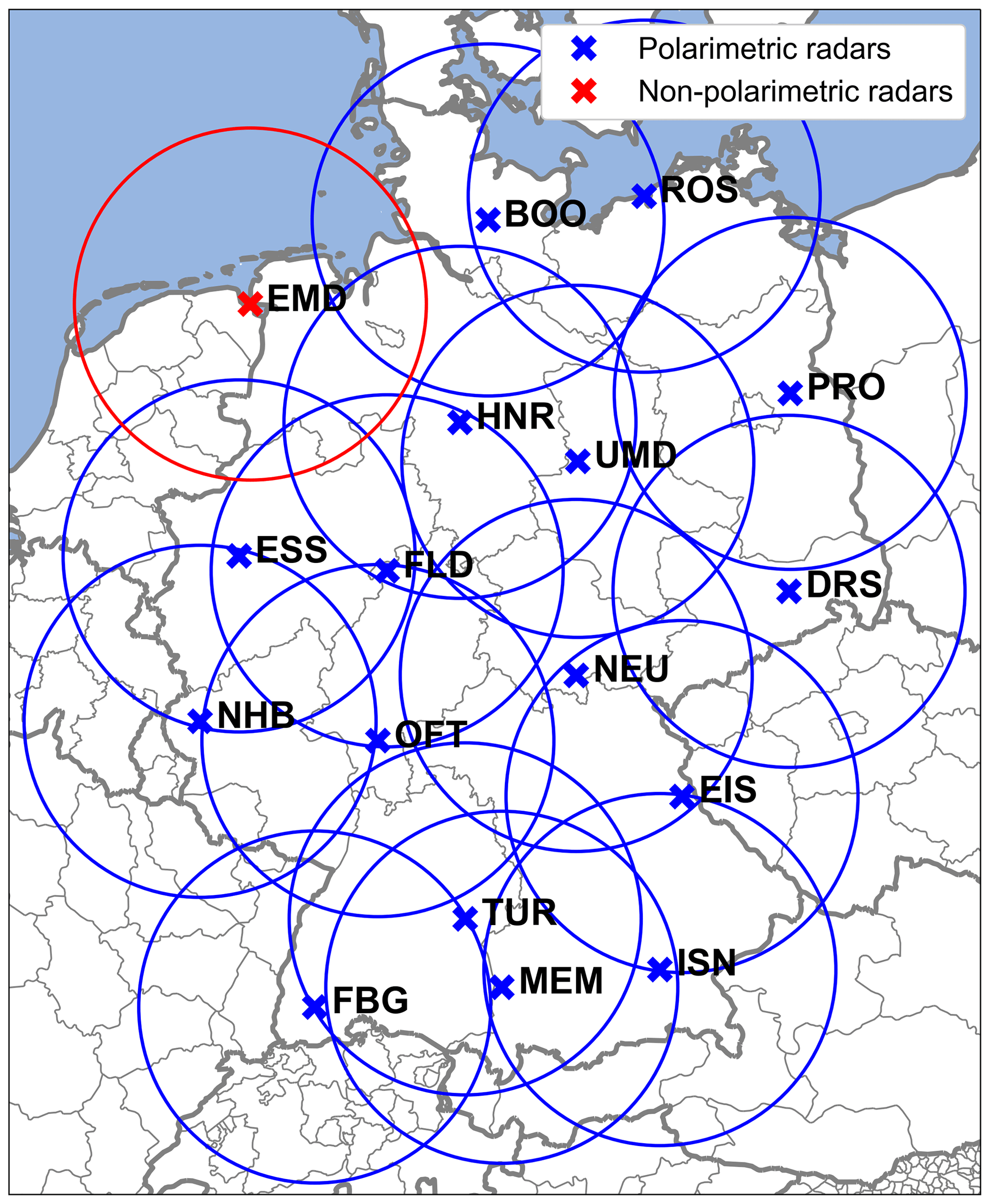
Figure 1 German polarimetric C-band radar network operated by DWD. Crosses indicate locations of radar stations in Emden (EMD), Boostedt (BOO), Rostock (ROS), Hannover (HNR), Ummendorf (UMD), Prötzel (PRO), Essen (ESS), Flechtdorf (FLD), Dresden (DRS), Neuhaus (NEU), Neuheilenbach (NHB), Offenthal (OFT), Eisberg (EIS), Türkheim (TUR), Isen (ISN), Memmingen (MEM), and Feldberg (FBG), circles indicate approximate ranges of 150 km around radars; blue color indicates polarimetric and red color indicates nonpolarimetric radars.

3 Data sets and microphysical retrievals

Intense summer precipitation events can pose a serious risk to society in Central Europe and are particularly difficult to forecast (Olson et al., 1995). Thus, we focus on three intense summer precipitation events in Germany. The first event covers a 2 d period of heavy, mostly stratiform precipitation over western Germany and its neighboring states from 13 to 14 July 2021, resulting from a slow-moving low-pressure system and causing devastating flooding, e.g., along the Ahr river in North Rhine-Westphalia (case S2021). The second event covers a 3 d period from 24 to 26 July 2017, characterized by widespread intense, mostly stratiform precipitation. It also caused flooding, especially in Lower Saxony in central-northern Germany along the Bode River catchment (case S2017). The third event dominated by convective precipitation covers a 1.5 d period from midday on 19 to 20 July 2017 (case C2017).

3.1 Radar observations

The DWD operates a network of 16 polarimetric C-band radars (blue circles in Fig. 1) and one additional nonpolarimetric radar (red circle). In “volume-scan” mode, the network monitors data consisting of Plan Position Indicators (PPI) at 10 radar elevation angles between 0.5 and 25^∘ with maximum slant ranges of about 180 km every 5 min. The data have a resolution of 1 km in range, which increased to 0.25 km in March 2021, and 1^∘ in azimuth; they are taken from the DWD archive.

For the direct assimilation of 3D Z data employed in this study, we use pre-processed Z observations including quality assurance and attenuation correction. For the LWC/IWC estimation, we use the raw polarimetric moments Z (given in dBZ), differential reflectivity Z_DR (given in dB), total differential phase Φ_DP (given in degrees), and co-polar cross-correlation coefficient ρ_HV. Z_DR is the logarithmic ratio between the backscattered power at horizontal and vertical polarizations, which is 0 dB for isotropic scatterers and shows larger positive values for oblate particles and negative values for prolate particles. Φ_DP is the lag in degrees of the horizontally polarized electromagnetic wave behind the vertically polarized one as the radar signal propagates through the atmosphere filled with anisotropic scatterers such as raindrops. Typically, half the range-derivative of Φ_DP, the specific differential phase shift K_DP (given in degrees per kilometer), is considered, which is positive for radar volumes filled with oblate particles and is affected by the presence of liquid water. ρ_HV is the cross-correlation coefficient between the horizontally and vertically polarized waves and is thus a measure of the diversity of scatterers in a radar volume. ρ_HV decreases in the presence of a pronounced diversity of hydrometeor shapes and in the presence of nonmeteorological targets, making it a useful tool for radar data quality assurance.

Kumjian (2013) notes that ρ_HV can be as low as 0.85 for snow/ice and 0.95 for rain at S-band. Here, we assume these values for C-band too. Thus, we only consider data below/above the melting layer for ${\mathit{\rho }}_{\mathrm{HV}}>\mathrm{0.95}/\mathrm{0.85}$ with ρ_HV corrected for noise before filtering (Ryzhkov and Zrnic, 2019). The height of the melting layer is determined from so-called Quasi-Vertical Profiles (i.e., azimuthal medians of PPIs measured at sufficiently high elevations and transferred to range-height displays; Trömel et al., 2014; Ryzhkov et al., 2016), as derived from PPIs of ρ_HV measured at a 5.5^∘ elevation angle, or from the nearest operational DWD radio sounding, especially in convective situations. K_DP is estimated from the filtered and smoothed Φ_DP following Vulpiani et al. (2012) with a fixed window size of 9 km. This window size is required because of the rather coarse radial resolution (1 km) for most of the PPIs considered to keep noise low and reduce potentially negative K_DP estimates. The horizontal specific attenuation A (given in dB km⁻¹) – the rate at which power is lost from the transmitted radar signal in horizontal polarization as it propagates through the precipitating atmosphere – is derived below the melting layer using the filtered and smoothed Φ_DP and measured (attenuated) Z using the ZPHI method (Testud et al., 2000). In the retrieval algorithms, the attenuation parameter α (ratio between A and K_DP, given in dB ^∘−1) is optimized for each ray using the self-consistency method proposed by Bringi et al. (2001). Finally, the raw Z and Z_DR data are corrected for (differential) attenuation using the optimized/climatological α values below/above the melting layer and the climatological value for the differential attenuation parameter β at C-band 0.02 dB ^∘−1 (Ryzhkov and Zrnic, 2019). For more details on the polarimetric radar moments, see, for example, Kumjian (2013).

3.2 Hybrid liquid water content retrieval

The LWC is estimated from the polarimetric radar observations below the melting layer following the hybrid retrieval proposed by Reimann et al. (2021) developed based on a large pure-rain disdrometer dataset and T-matrix scattering calculations at C-band. The estimator combines different polarimetric radar moments to optimally exploit and mitigate respective advantages and disadvantages known for different precipitation characteristics. For example, in weak precipitation indicated by small total Φ_DP increments ΔΦ_DP<5^∘ below the melting layer, the LWC(Z,Z_DR) relation is used (LWC is always in g m⁻³):

$$\begin{array}{}\text{(2a)}& {\log }_{\mathrm{10}}\left(\mathrm{LWC}\left(Z,Z_{\mathrm{DR}}\right)\right)=\mathrm{0.058}Z-\mathrm{0.118}{Z}_{\mathrm{DR}}-\mathrm{2.36}.\end{array}$$

In such situations, K_DP is potentially noisy owing to noise in Φ_DP and A potentially suffers from an unreliable ΔΦ_DP estimation, whereas the influence of (differential) attenuation on Z and Z_DR should be small for these rays. For stronger rain – rays with ΔΦ_DP>5^∘ – the negative influence of (differential) attenuation on Z and Z_DR increases, whereas less noise and uncertainty is expected in K_DP and A; therefore, LWC(A) and LWC(K_DP) estimators are used. The LWC(A) estimator

$$\begin{array}{}\text{(2b)}& {\log }_{\mathrm{10}}\left(\mathrm{LWC}\right(A\left)\right)=-\mathrm{0.1415}{\log }_{\mathrm{10}}(A{)}^{\mathrm{2}}+\mathrm{0.209}{\log }_{\mathrm{10}}(A)+\mathrm{0.46},\end{array}$$

is used for radar bins with Z<45 dBZ, when hail is unlikely, and the LWC(K_DP) estimator

$$\begin{array}{}\text{(2c)}& {\log }_{\mathrm{10}}\left(\mathrm{LWC}\left(K_{\mathrm{DP}}\right)\right)=\mathrm{0.568}{\log }_{\mathrm{10}}\left(K_{\mathrm{DP}}\right)+\mathrm{0.06},\end{array}$$

is used for bins with Z>45 dBZ, as K_DP is less affected by hail than A. In addition, resonance scattering of medium and large raindrops at C-band may favor the use of LWC(K_DP) compared with LWC(A) in moderate to heavy rain. It should be noted, however, that the hybrid LWC estimator is likely unsuitable in the presence of hail and graupel, especially in certain convective situations, owing to its derivation from pure-rain observations.

3.3 Hybrid ice water content retrieval

The IWC is estimated above the melting layer using the hybrid estimator proposed by Carlin et al. (2021). It combines the relations based on Z_DR and K_DP (Ryzhkov and Zrnic, 2019)

$$\begin{array}{}\text{(3a)}& \mathrm{IWC}\left(z_{\mathrm{DR}},K_{\mathrm{DP}}\right)=\mathrm{4.0}\times {\mathrm{10}}^{-\mathrm{3}}{\displaystyle \frac{K_{\mathrm{DP}}\mathit{\lambda }}{\mathrm{1}-z_{\mathrm{DR}}^{-\mathrm{1}}}},\end{array}$$

with the one based on Z and K_DP (Bukovcic et al., 2018, 2020)

$$\begin{array}{}\text{(3b)}& \mathrm{IWC}\left(z,K_{\mathrm{DP}}\right)=\mathrm{3.3}\times {\mathrm{10}}^{-\mathrm{2}}{\left(K_{\mathrm{DP}}\mathit{\lambda }\right)}^{\mathrm{0.67}}{z}^{\mathrm{0.33}},\end{array}$$

with z and z_DR are Z and Z_DR given in linear units (mm⁶ m⁻³ and unitless), IWC in g m⁻³, and the radar wavelength λ set to 53 mm (C-band). The estimators in Eq. (3) are again combined to complement their individual strengths: Eq. (3a) is fairly immune to the orientation and shape of snowflakes, but sensitive to variations in ice density and prone to errors from Z_DR biases especially at low Z_DR values; Eq. (3b) is immune to Z_DR miscalibration, but sensitive to hydrometeor aspect ratio, orientation, and density. Equation (3a) is used for Z_DR>0.4 dB and Eq. (3b) otherwise. Recently, Blanke et al. (2023) demonstrated the high accuracy of this hybrid estimator (correlation coefficient and root-mean-square deviation 0.96 and 0.19 g m⁻³, respectively) in an evaluation study with in situ airplane observations on the west coast of the USA. It should be noted, however, that both parts of the hybrid IWC estimator in Eq. (3) are adapted to snowfall, with their derivation based on an inversely proportional relationship between particle density and diameter, which usually does not hold for hail and graupel. Therefore, its applicability to hail and/or graupel in convective situations in particular may be limited.

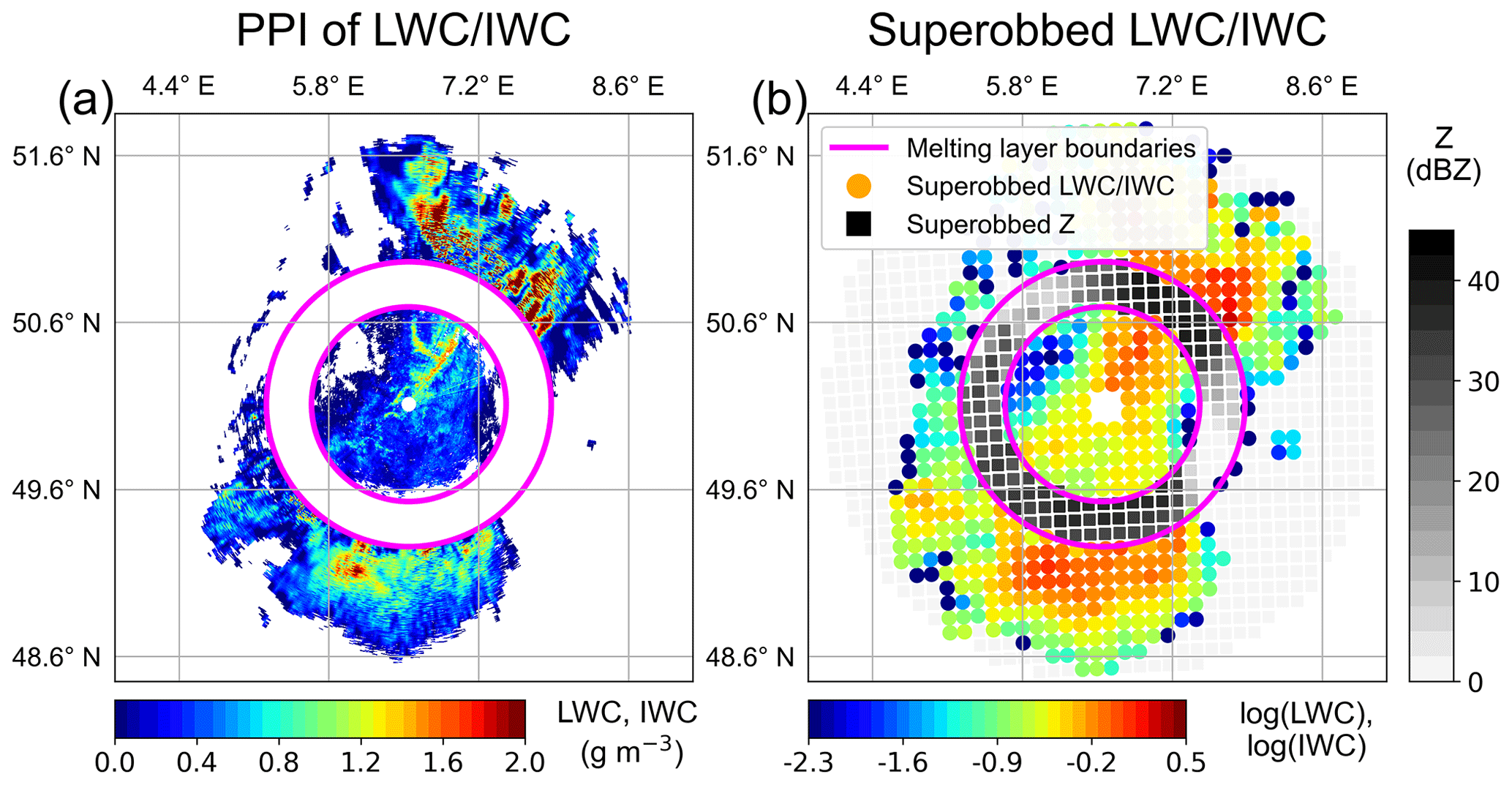
Figure 2 Visualization of the superobbing process from (a) a PPI of estimated LWC (Eq. 2) below and IWC (Eq. 3) above the melting layer (approximate upper and lower boundaries of the melting layer indicated by violet rings) at 1.5^∘ of the DWD radar NHB (see Fig. 1) for the stratiform precipitation case S2021 on 14 July 2021 16:00 UTC to (b) the corresponding field of superobbed (with the pre-selected settings winsize_avg = 10 km, lower_lim = −2.3, and minnum_vals = 3) log(LWC) and log(IWC) (colored dots) and superobbed reflectivity Z (gray squares), where no LWC/IWC estimates are available (e.g., within the melting layer).

4 Setup of assimilation experiments

4.1 Retrieval resolution

The retrieved LWC and IWC values with the resolution corresponding to the measured radar data are subjected to “superobbing” (see an example in Fig. 2), which is also applied to the Z data in KENDA. Superobbing reduces the resolution of the radar data to approximately match the resolution of the analysis grid by spatial and elevation-wise averaging in the linear scale to a Cartesian grid with a resolution (res_cartesian in kilometers) corresponding to the analysis grid (10 km for an analysis grid coarsening factor of three currently used in KENDA). The number of radar bins contributing to the averaging decreases with increasing distance from the radar, and the window size for the averaging (winsize_avg in kilometers) is equal to res_cartesian in KENDA, but is also modified in our study while keeping res_cartesian constant. The minimum number of valid values in the superobbing window to perform superobbing (minnum_vals) is three observations, as used for the 3D Z DA in KENDA. Further details on the superobbing procedure can be found in Bick et al. (2016) and Zeng et al. (2021).

The LWC and IWC estimates are assimilated with a lower limit (lower_lim) similar to the “no-precipitation” threshold of 0 dBZ used for the Z assimilation in KENDA. In contrast to Z, the LWC and IWC data in no-precipitation are mostly filtered out by the applied ρ_HV thresholds, but such a lower data threshold can still be useful to limit the variability in the microphysical estimates and thus can also be used for tuning (personal communication with Ulrich Blahak, DWD). We choose lower_lim = −2.3 for log ₁₀(LWC), which approximately corresponds to 0 dBZ for Z when comparing measured log ₁₀(LWC) and synthetic Z data obtained from T-matrix scattering calculations for a large German pure-rain disdrometer data set (not shown). The rare occurrence of snow on the ground in Germany and instrumental limitations prevent a similar analysis for IWC. Therefore, we also use −2.3 for log ₁₀(IWC).

Analogous to the assimilation of 3D Z data in KENDA, only the PPIs at radar elevation angles of 1.5, 3.5, 5.5, 8.0, and 12.0^∘ are used for LWC and IWC, and data from altitudes below 600 and above 9000 m are not considered. The superobbed microphysical estimates are assimilated in the logarithmic scale, similar to the Z data in KENDA, which leads to better results than assimilating the data in the linear scale (not shown; e.g., Liu et al., 2020).

4.2 Assimilation settings and first guess

Z is currently assimilated in KENDA with a fixed observation error standard deviation (obserr_std) of 10 dBZ. We use a fixed value of obserr_std = 0.5, which can be obtained statistically from the disdrometer data considered above: a difference Δlog ₁₀(LWC) = 0.5 covers a similar fraction of the full range of data as ΔZ=10 dBZ (not shown). This value is also used for log ₁₀(IWC). The horizontal observation localization length-scale (obsloc_hor) and the vertical observation localization length-scale (obsloc_ver) are set to 16 km and to increase with height from 0.075 to 0.5 in the logarithm of pressure (ln (p)) as used for the 3D Z DA in KENDA. Moreover, microphysical analysis increments of only cloud water mixing ratio and specific humidity are produced, i.e., not all available hydrometeor species (e.g., rain, cloud ice, and graupel mixing ratios) are updated individually in KENDA's standard configuration.

Table 1 Pre-selected and modified (modifications 1 and 2) values for the DAPs obsloc_hor (horizontal observation localization length-scale in kilometers), obsloc_ver (vertical localization length-scale in the logarithm of pressure ln (p)), obserr_std (observation error standard deviation for log(LWC) and log(IWC)), winsize_avg (superobbing window size in kilometers), lower_lim (lower limit of the log(LWC) and log(IWC) data), and minnum_vals (minimum number of valid values for superobbing).

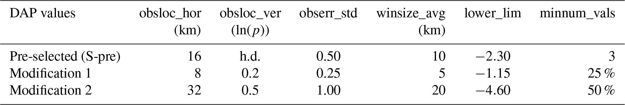
Figure 3 Exceedances of hourly rain accumulation thresholds 0.5 (black curves), 1.0 (green), 2.0 (blue), and 4.0 mm h⁻¹ (yellow) in the RADOLAN data (hourly accumulations) for the rainfall cases (a) C2017, (b) S2017, and (c) S2021 as percentages of the total number of threshold exceedances in all three rainfall cases and thresholds considered. The fractions are used to determine weights for calculations of weighted medians of FSS and BSS (e.g., in Fig. 4), and for the calculation of the univariate measure JQS (see Eq. 5 in Sect. 4.4).

First guesses of LWC and IWC are calculated with a simple “forward operator”, which uses the prognostic model variables total air density (ρ_tot, given in kg m⁻³) and the rain and cloud water mixing ratios q_r and q_c for LWC, and the snow, graupel, and cloud ice mixing ratios q_s, q_g, and q_i (all given in g m⁻³) for IWC at the model grid points via

$$\begin{array}{}\text{(4a)}& \mathrm{LWC}={\mathrm{10}}^{\mathrm{3}}{\mathit{\rho }}_{\mathrm{tot}}\left(q_{\mathrm{r}}+q_{\mathrm{c}}\right),\end{array}$$

and

$$\begin{array}{}\text{(4b)}& \mathrm{IWC}={\mathrm{10}}^{\mathrm{3}}{\mathit{\rho }}_{\mathrm{tot}}\left(q_{\mathrm{s}}+q_{\mathrm{g}}+q_{\mathrm{i}}\right).\end{array}$$

The first-guess LWCs and IWCs are then projected using the nearest-neighbor method onto the polar (PPI) grid of the observed LWC and IWC data and superobbed analogously to the observed data. This procedure is done for the ensemble and the deterministic run.

4.3 Model initialization and lateral boundary data

ICON-D2 model data in 40 + 1-mode for our evaluation periods are provided by DWD for the initial times of the experiment periods 00:00 UTC 13 July 2021, 00:00 UTC 24 July 2017, and 11:00 UTC 19 July 2017. These data are outputs from the regular ICON-D2 routine and thus do not require further “spin-up” integrations prior to our assimilation experiments. ICON-EU model data provided by DWD are used as lateral boundary conditions every hour.

4.4 Experiment part A: assimilation configurations

From the model initial times, 3D LWC and IWC estimates are assimilated in hourly assimilation cycles instead of 3D Z data, where available, to avoid potential problems arising from assimilating the information from the Z data twice. Thus, Z data is always assimilated within the melting layer and in precipitation-free areas, where the LWC and IWC estimates are not available owing to the applied ρ_HV thresholds. We exclude the assimilation of 3D V observations and LHN to focus on the assimilation of microphysical information from the radar network. We assimilate the LWC and IWC estimates separately to study their individual impact on weather forecasts, but also to identify individual best DA parameter (DAP; obsloc_hor, obsloc_ver, obserr_std, winsize_avg, lower_lim, and minnum_vals) sets. The DA configurations assimilating LWC and IWC also assimilate conventional observations and are therefore referred to as CNV + LWC$/Z$ and CNV + IWC$/Z$. The DA of only conventional observations and the DA of conventional and 3D Z observations are used as reference configurations CNV and CNV + Z, respectively.

Table 2 First and second near-random sample of DAP settings (S1-01 to S1-12 and S2-01 to S2-10) generated with Latin Hypercube Sampling from all the DAP values in Table 1 and with a reduced number of DAP values from Table 1 based on consideration of the univariate measure JQS_v (see Eq. 5 in Sect. 4.4) calculated with the first sample, respectively.

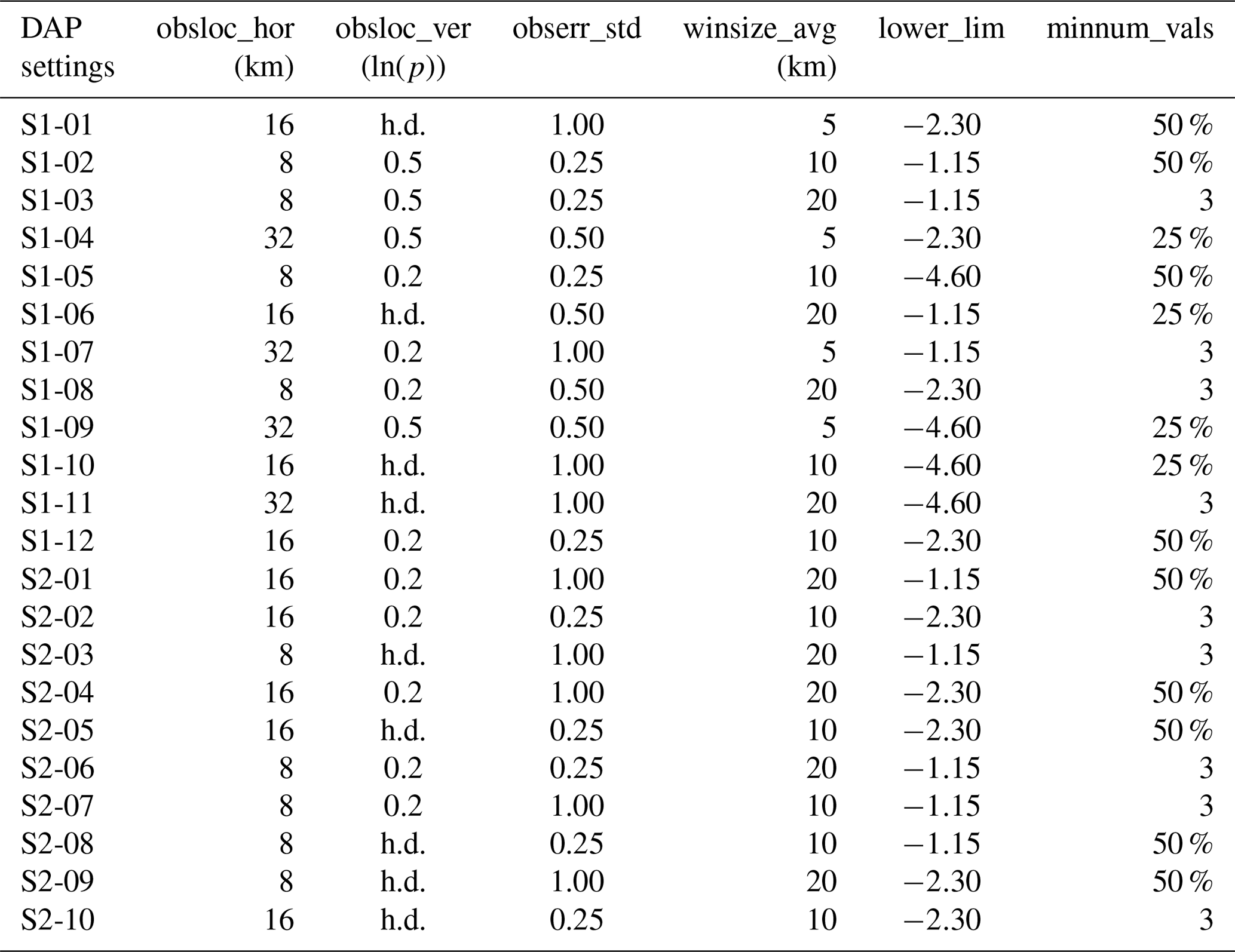
We consider a near-random sample of DAP settings generated via Latin Hypercube Sampling (LHS) by modifying the DAP values from their pre-selected values (pre-selected and modified values in Table 1; generated settings S1-01 to S1-12 in Table 2). The results of using the DAP configurations or values are compared with each other in terms of both first-guess deterministic and ensemble QPF quality via a single univariate measure newly introduced here – the joint quality score (JQS):

$$\begin{array}{}\text{(5)}& \begin{array}{rl}{\mathrm{JQS}}_{\mathrm{c}/\mathrm{v}}& ={\mathrm{median}}_{\mathrm{w}}\left({\mathrm{\Delta }}_{\mathrm{CNV}+Z}{\mathrm{FSS}}_{\mathrm{norm}}\left[\mathrm{CNV}+X/Z\right]\right)\\ & +{\mathrm{median}}_{\mathrm{w}}\left({\mathrm{\Delta }}_{\mathrm{CNV}+Z}{\mathrm{BSS}}_{\mathrm{norm}}[\mathrm{CNV}+X/Z]\right).\end{array}\end{array}$$

Although changes in deterministic and ensemble QPF quality with respect to the CNV + Z configuration are not always consistent, the JQS provides a useful measure for the overall intercomparison of DA settings. In Eq. (5), FSS is the deterministic Fraction Skill Score (Roberts and Lean, 2008), BSS is the Brier Skill Score (following Wilks, 2019 and Bick et al., 2016) quantifying the ensemble forecast quality, and both quantities are calculated using DWD's RADOLAN (Radar-Online-Aneichung) product (https://opendata.dwd.de/climate_environment/CDC/grids_germany/hourly/radolan/historical/bin/, last access: 17 November 2022) as verification data; Δ_CNV+Z denotes differences with respect to the CNV + Z configuration; X is LWC or IWC; index “norm” denotes normalization with the means of ${\mathrm{\Delta }}_{\mathrm{CNV}+Z}\mathrm{FSS}[\mathrm{CNV}+Z]$ or ${\mathrm{\Delta }}_{\mathrm{CNV}+Z}\mathrm{BSS}[\mathrm{CNV}+Z]$; median_w (…) denotes the weighted median. Medians are used instead of means in order to reduce the impact of outliers in FSS and BSS, and weights are determined by the fractions of threshold exceedances for a given time and threshold of the total number of exceedances at all thresholds (0.5, 1.0, 2.0, and 4.0 mm h⁻¹) and events (C2017, S2017, and S2021) in the RADOLAN data (see Fig. 3). We use weighted medians over all cases and thresholds to compare QPF quality between different DAP configurations (JQS_c) and additionally calculate weighted medians over all DAP settings that have the same DAP values to compare individual DAP values (JQS_v).

In addition to optimizing DAP sets in terms of first-guess quality, we also aim to optimally combine the radar data sets considered (i.e., Z, LWC, and IWC). Therefore, also the parallel assimilation of LWC or IWC and Z (configurations CNV + LWC + Z or CNV + IWC + Z respectively), the combined assimilation of LWC and IWC estimates as alternatives to Z (configuration CNV + [LWC + IWC]$/Z$) or in parallel to Z (CNV + LWC + IWC + Z) are also evaluated with JQS_c.

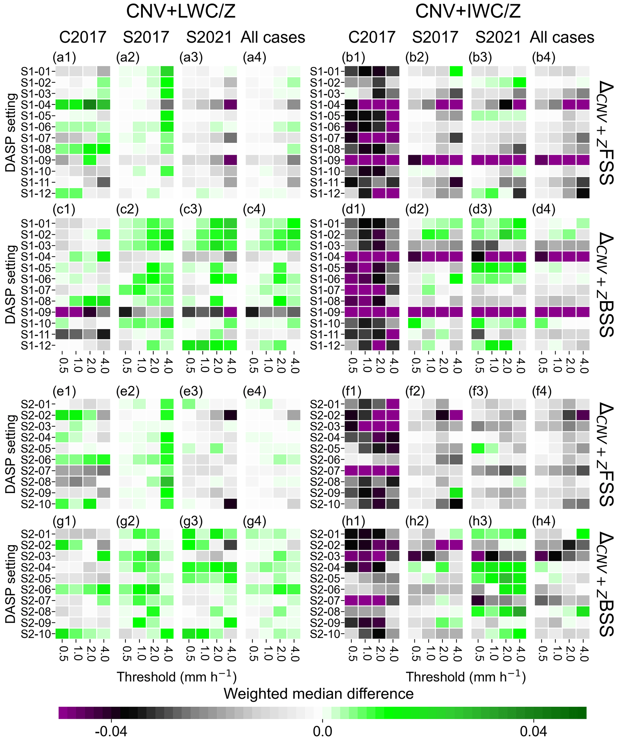
Figure 4 Weighted medians of differences in first-guess deterministic FSS (first and third panel rows) and BSS (second and fourth panel rows) between the CNV + LWC$/Z$ (left block) or CNV + IWC$/Z$ (right block) configurations with different sampled DAP settings (S1-01 to S1-12 and S2-01 to S2-10 in Table 2) and the CNV + Z configuration for accumulation thresholds 0.5, 1.0, 2.0, and 4.0 mm h⁻¹ and the three rainfall periods considered (three left columns within each block). The right-most column in each block shows the weighted median over all cases considered. Weights are determined by threshold exceedances in the RADOLAN data (see Fig. 3). Green color indicates improvements compared with the CNV + Z configuration, gray to dark purple color indicates degradations.

4.5 Experiment part B: 9 h forecasts

Finally, the impact of assimilating the 3D microphysical estimates with KENDA on forecasts with lead times greater than 1 h is evaluated. The 3D LWC and IWC estimates are assimilated with the identified DAP sets and radar data set configurations that lead to the best first-guess QPF quality in hourly assimilation cycles, as before, and then 9 h deterministic forecasts of the ICON-D2 model are initiated every third hour from the produced analyses. The quality of the deterministic 9 h QPF is assessed using the FSS and the Frequency Bias (FBI; e.g., Bick et al., 2016). Probabilistic forecasts are not considered owing to data storage limitations.

5 Numerical results

5.1 Experiment part A: assimilation configurations

The CNV + LWC$/Z$ configuration yields different first-guess FSS and BSS values for the different DAP settings (see Table 2) and precipitation cases (Fig. 4a and c). Improvements over the CNV + Z configuration considering all cases together are obtained, e.g., with the DAP sets S1-01 to S1-03, or S1-06 (Fig. 4a4 and c4). These best-performing sets all have rather small horizontal observation localizations obsloc_hor of 8 and 16 km and rather high lower limits lower_lim of −1.15 and −2.30 (see Table 2). Similarly, the CNV + IWC$/Z$ configuration also yields different first-guess FSS and BSS values for different DAP sets (Table 2) and precipitation cases (Fig. 4b and d). Improvements over the CNV + Z configuration are mostly limited to the 2021 stratiform case, e.g., for the DAP settings S1-02 or S1-05 (Fig. 4b3 and d3), whereas first-guess QPF is mostly degraded for the 2017 convective case (Fig. 4b1 and d1).

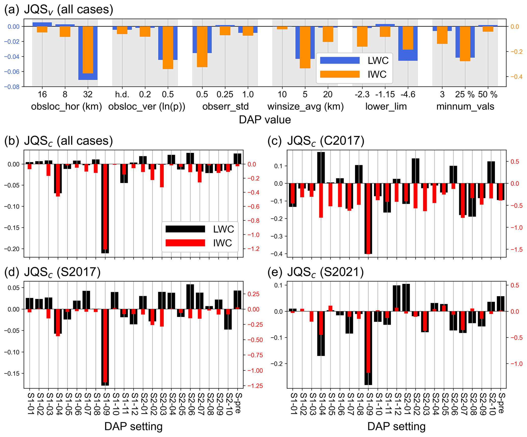
Figure 5 (a) Comparison of the investigated DAP values for obsloc_hor, obsloc_ver, obserr_std, winsize_avg, lower_lim, and minnum_vals (Table 1) in terms of the univariate measure JQSv (see Eq. 5 in Sect. 4.4) for the LWC (blue bars) and IWC (orange bars) assimilation with the DAP settings from the first DAP settings (S1-01 to S1-12 in Table 2). In (b), all 22 DAP settings (S1-01 to S1-12 and S2-01 to S2-10 in Table 2) plus the pre-selected DAP setting (setting S-pre in Table 1) are compared with each other in terms of the univariate measure JQSc (see Eq. 5 in Sect. 4.4) for the LWC (black bars) and IWC (red bars) assimilation considering all rainfall cases together. Panels (c)–(e) are like panel (b), but with the JQSc calculated for the individual rainfall cases C2017, S2017, and S2021, respectively.

The univariate measure JQS_v (see Sect. 4.4 and Eq. 5), which uses the first-guess FSS and BSS values, is used to find the best DAP settings for LWC and IWC in terms of first-guess QPF quality. The DAP values obsloc_hor = 32 km, obsloc_ver = 0.5ln (p), obserr_std = 0.5, winsize_avg = 5 km, lower_lim = −4.6, and minnum_vals = 25 % (i.e., 25 % of the radar pixels in the superobbing window must have valid values) give the worst (and negative) JQS_v values for both LWC and IWC (blue and orange bars in Fig. 5a). Another 10 DAP sets in the vicinity of the better performing ones are sampled with LHS (S2-01 through S2-10 in Table 2). Further improvements over the CNV + Z configuration are obtained for the LWC assimilation (Fig. 4e and g), but are mostly only obtained for the 2021 stratiform case for the IWC assimilation (Fig. 4f3 and h3). The new DAP settings (Table 2; Fig. 4e–h) do, however, on average not perform significantly better than the first sample (Table 2; Fig. 4a–d), except that strong negative outliers (e.g., S1-09 in Fig. 4a–d) no longer appear.

The 22 DAP settings (Table 2) for the LWC and IWC assimilations are compared with each other in terms of first-guess deterministic and ensemble QPF quality using the univariate measure JQS_c (see Sect. 4.4 and Eq. 5). Several DAP settings for the LWC assimilation yield positive JQS_c values (black bars in Fig. 5b) and thus improved first-guess FSS and BSS values compared with the CNV + Z configuration, whereas for the IWC assimilation, positive JQS_c values are limited to the 2021 stratiform case (red bars in Fig. 5e). The DAP set S2-06 (obsloc_hor = 8 km, obsloc_ver = 0.2ln (p), obserr_std = 0.25, winsize_avg = 20 km, lower_lim = −1.15, and minnum_vals = 3, see Table 2) for LWC yields overall the best JQS_c (black bars Fig. 5b), whereas setting S1-02 (obsloc_hor = 8 km, obsloc_ver = 0.5ln (p), obserr_std = 0.25, winsize_avg = 10 km, lower_lim = −1.15, and minnum_vals = 50 %, see Table 2) results in the best (but rather neutral) JQS_c value for IWC (red bars in Fig. 5b).

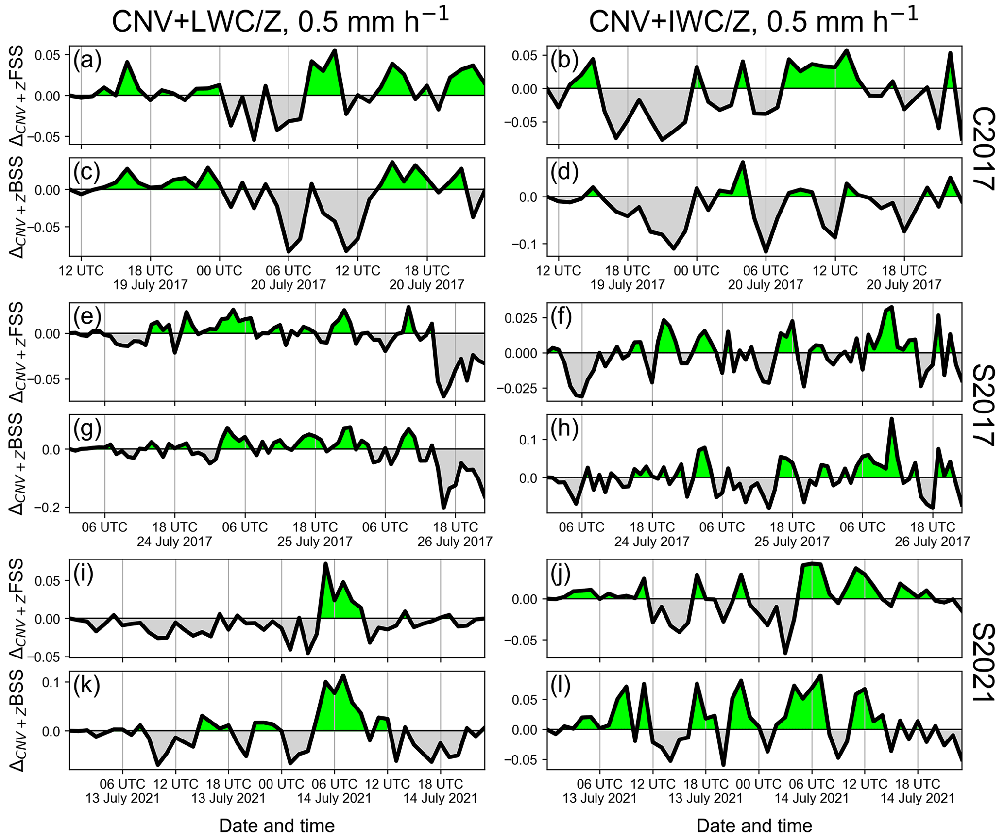
Figure 6 Time series of the difference in first-guess deterministic FSS and BSS for a threshold of 0.5 mm h⁻¹ between the CNV + LWC$/Z$ (a, c, e, g, i, k) or CNV + IWC$/Z$ (b, d, f, h, j, l) configurations and the CNV + Z configuration using the best-performing DAP settings found for LWC and IWC (S2-06 and S1-02, see Table 2) with respect to first-guess quality in hourly assimilation cycles for the precipitation cases (a–d) C2017, (e–h) S2017, and (i–l) S2021. Green shading indicates improvements with respect to CNV + Z, gray shading indicates deteriorations.

The assimilation of LWC (CNV + LWC$/Z$) with the respective best DAP setting in terms of first-guess quality improves first-guess QPF for the 2017 precipitation cases (Fig. 4e1, e2, g1, g2 and black bars in Fig. 5c and d) compared with the CNV + Z configuration, whereas QPF quality is degraded for the stratiform S2021 case (Fig. 4e3, g3 and black bars in Fig. 5e). As expected, the time series of the first-guess FSS and BSS values at a threshold of 0.5 mm h⁻¹ show slight, systematic improvements for the 2017 cases for some time intervals (green colors in Fig. 6a, c, e, and g), but more pronounced degradations for the 2021 case (Fig. 6i and k). The assimilation of IWC (CNV + IWC$/Z$) with the respective best DAP set yields improvements over the CNV + Z configuration particularly for the stratiform S2021 case (Fig. 4b3, d3 and red bars in Fig. 5e), but clear quality decreases for the convective C2017 case (Fig. 4b1, d1 and red bars in Fig. 5c). Time series of first-guess FSS and BSS values at a 0.5 mm h⁻¹ threshold confirm this finding: slight, systematic improvements are evident for the 2021 case in some time periods (Fig. 6j and l), whereas degradations are visible for the 2017 convective case (Fig. 6b and d). The better performance of the IWC assimilation for the 2021 stratiform case may be due the higher radial resolution of the more recent radar data of DWD (recall that the resolution was increased from 1 km to 0.25 km in spring 2021), which leads to better K_DP estimates, because many more consecutive radar bins are considered for the 9 km K_DP-estimation window used. Using the same window length for the lower-resolution data for the 2017 cases means using only one quarter of the data compared with the 2021 case. Estimating K_DP from only nine consecutive values may favor negative K_DP estimates resulting in negative IWC values, which are set to the lower limit (lower_lim) value in the superobbing procedure and are thus treated as “no-precipitation”. The replacement of negative IWC estimates with zero or with the IWC(Z) retrievals following Atlas et al. (1995) led to some improvements, but the first-guess QPF quality remained below the CNV + Z configuration (not shown).

Parallel assimilation of LWC and Z (CNV + LWC + Z), i.e., assimilation of LWC and Z at the same superobbing points, reduces the JQS_c values compared with the alternative assimilation strategy (CNV + LWC$/Z$), but is still better than the CNV + Z configuration (lower black bars in Fig. 7). In contrast, the parallel assimilation of IWC and Z (CNV + IWC + Z) improves JQS_c values compared with the alternative assimilation strategy (CNV + IWC$/Z$; middle black bars in Fig. 7) above the CNV + Z quality. Assimilation of all radar data sets in parallel (CNV + LWC + IWC + Z) gives the best JQS_c value (upper black bar in Fig. 7b).

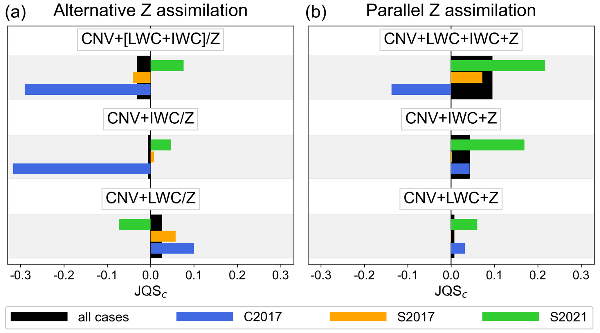
Figure 7 Comparison of different radar data set configurations in terms of the univariate measure JQS_c (see Eq. 5 in Sect. 4.4). Configurations assimilating LWC and/or IWC with the best DAP settings found (S2-06 and S1-02 in Table 2) in terms of first-guess QPF quality (a) instead of Z where possible (alternative Z assimilation) in configurations CNV + LWC$/Z$, CNV + IWC$/Z$, and CNV + [LWC + IWC]$/Z$ (lower, middle, and upper bars), and (b) together with Z (parallel Z assimilation) in configurations CNV + LWC + Z, CNV + IWC + Z, and CNV + LWC + IWC + Z (lower, middle, and upper bars) are compared. Black bars indicate the JQS_c calculated over all three rainfall cases, and blue, orange, and green bars indicate the JQS_c calculated over the individual cases C2017, S2017, and S2021 respectively.

The impact of the LWC and IWC assimilation on the first-guess of temperature, relative humidity, and u-wind speed is investigated using conventional observations. The assimilation of radar information generally reduces standard deviations (SD) compared with the assimilation of only conventional data (CNV + Z, CNV + LWC$/Z$, CNV + IWC$/Z$, and CNV + LWC + IWC + Z configurations correspond to black, red, yellow, and blue curves in Fig. 8b, e, and h), whereas the impact on mean bias deviations (MBD) is less clear (compare black solid, red, yellow, and blue curves with black dotted curves in Fig. 8c, f, and i). The CNV + LWC$/Z$, CNV + IWC$/Z$, and CNV + LWC + IWC + Z configurations result in SDs and MBDs similar to the CNV + Z configuration, but slight, systematic SD improvements are evident for the u-wind speed with the CNV + IWC$/Z$ configuration (yellow curve in Fig. 8h).

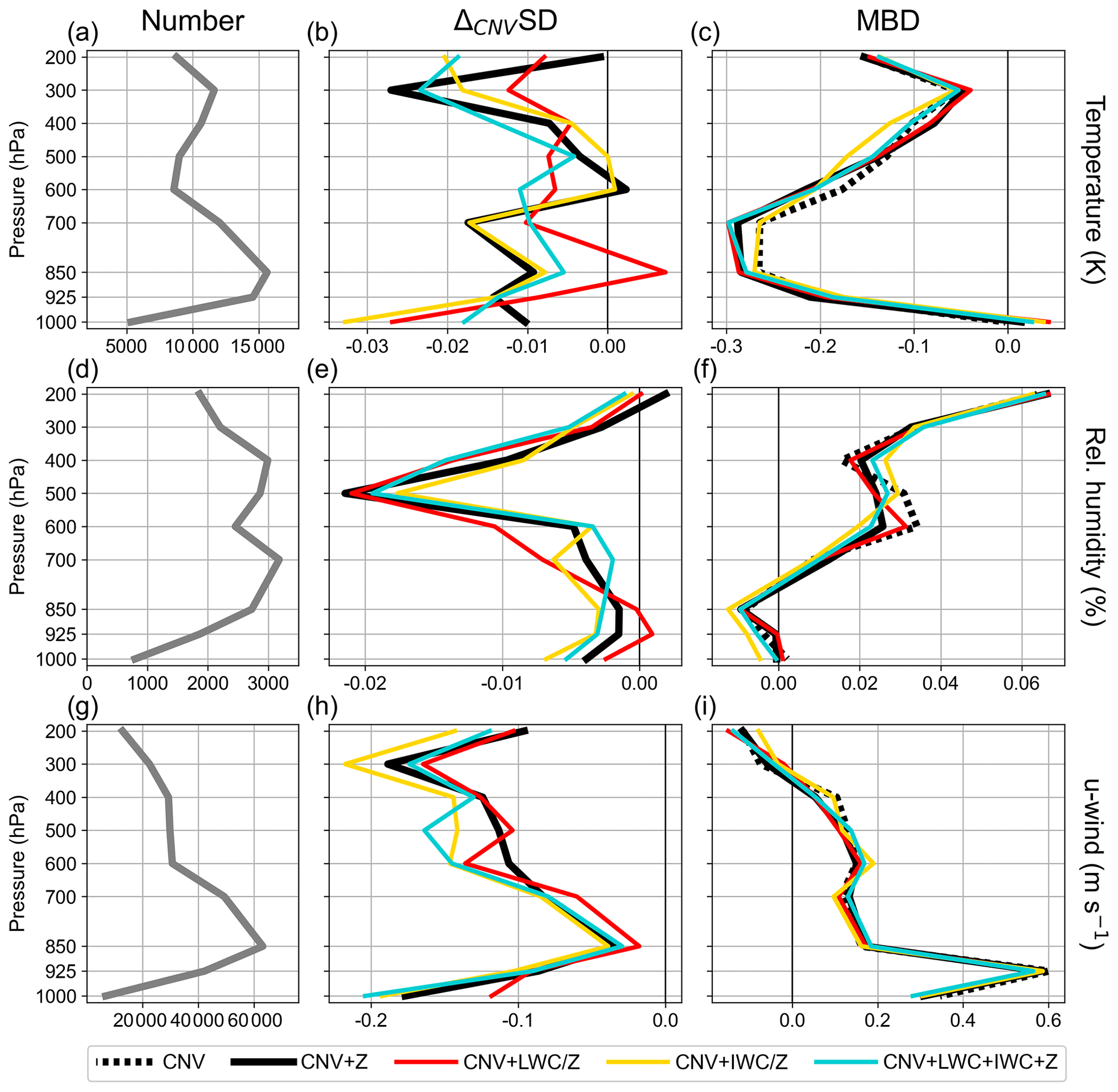
Figure 8 Vertical profiles of differences in standard deviations (SD) with respect to the CNV configuration (b, e, h) and of mean bias deviations (MBD; c, f, i) of first guesses of temperature (a–c), relative humidity (d–f), and u-wind (g–i) obtained from hourly assimilation cycles with the assimilation configurations CNV (black dotted), CNV + Z (black solid), CNV + LWC$/Z$ (red), CNV + IWC$/Z$ (yellow), and CNV + LWC + IWC + Z (blue curves) from conventional observations over Germany. The number of observations contributing to the SD and MBD calculations are shown in the left column (gray solid curves). All rainfall cases are considered and the best DAP settings found for LWC and IWC (S2-06 and S1-02 in Table 2) in terms of first-guess QPF quality are used for the LWC and IWC assimilations.

5.2 Experiment part B: 9 h forecasts

With the best performing DAP sets for the LWC and IWC assimilations in terms of first-guess QPF quality, up to 9 h forecasts are performed. Z observations (CNV + Z) clearly improve the deterministic FSS for a threshold of 0.5 mm h⁻¹ for all forecast hours compared with the assimilation of only conventional data (CNV) on average for all cases (compare black with gray lines in Fig. 9a, d, g, and j). This also holds for the deterministic FBI for the stratiform S2017 and S2021 cases, whereas for the convective C2017 case the underestimation is enhanced (compare black and gray curves in Fig. 9c, f, i, and l). Assimilating LWC estimates instead of Z data where possible (CNV + LWC$/Z$) slightly further improves the FSS on average over all cases for most of the forecast time (red curve above the zero line in Fig. 9b). This overall positive impact results from the first 6 h of the convective C2017 case and forecast hours five to nine of the stratiform 2021 case (Fig. 9e and k). FBI improvements are achieved for up to 7 h lead time (compare red with black curves in Fig. 9c) and at least for the first 4 h lead time for all individual cases (compare red curves with gray and black curves in Fig. 9f, i, and l).

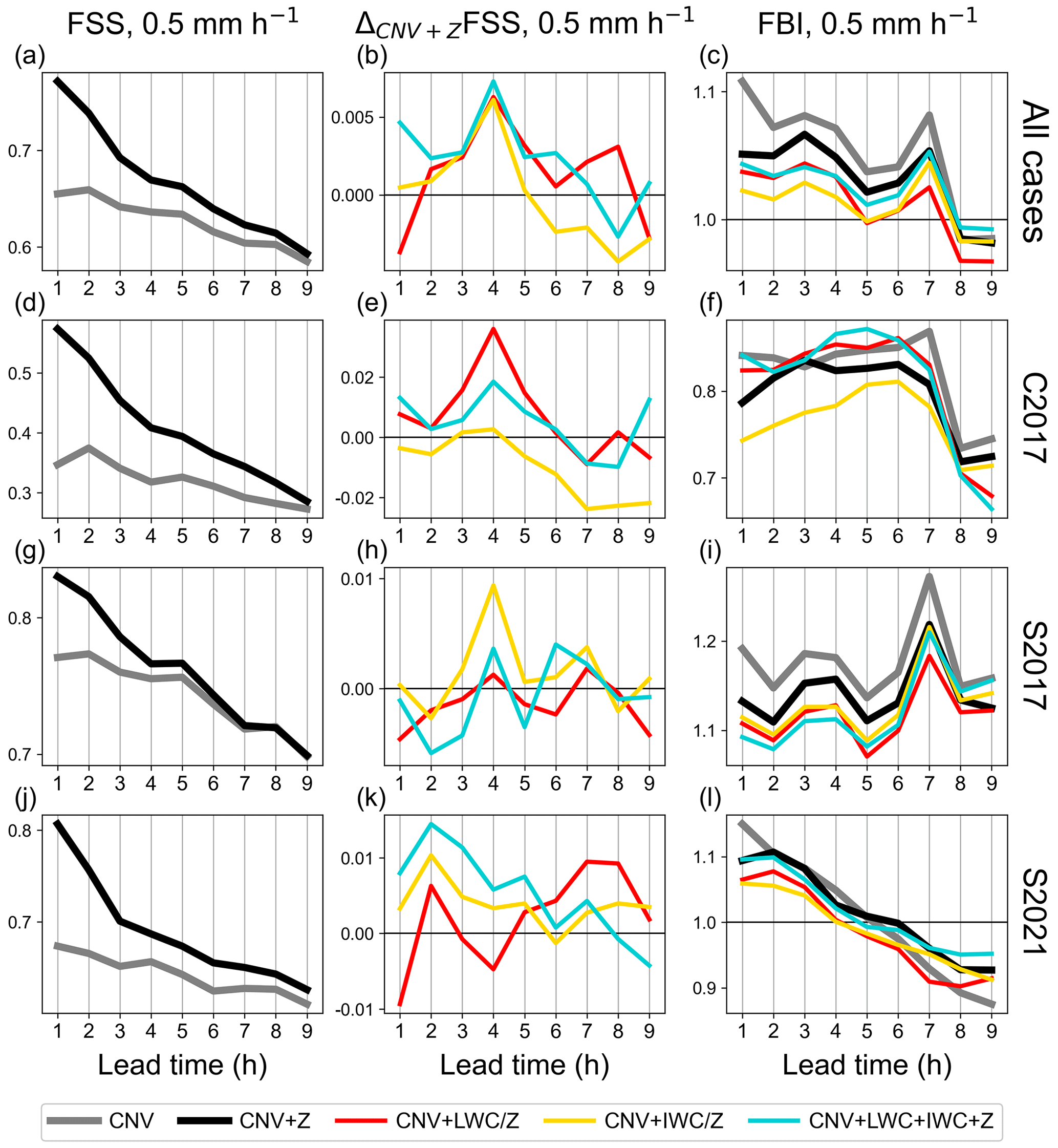
Figure 9 (a, d, g, j) Time series of the deterministic FSS for a 0.5 mm h⁻¹ threshold of 9 h forecasts initiated every third hour from hourly assimilation cycles with the CNV and CNV + Z configurations (gray and black curves) as means over all precipitation cases (a–c), over only the 2017 convective case C2017 (d–f), over only 2017 stratiform case S2017 (g–i), and over only the 2021 stratiform case S2021 (j–l). (b, e, h, k) Corresponding deviations in mean deterministic FSS from the CNV + Z configuration of the CNV + LWC$/Z$ (red curves), CNV + IWC$/Z$ (yellow curves), and CNV + LWC + IWC + Z (blue curves) configurations using the found best DAP settings for LWC and IWC assimilations (S2-06 and S1-01 in Table 2) in terms of first-guess QPF quality. (c, f, i, l) Corresponding mean deterministic FBI.

The IWC assimilation (CNV + IWC$/Z$) only marginally improves the FSS on average for the first 5 h lead time (yellow curves in Fig. 9b) compared with the CNV + Z configuration. As expected from the first-guess analysis, the mean FSS for the convective C2017 case is mostly degraded (yellow curve in Fig. 9e) and the stratiform S2017 and S2021 cases are improved (yellow curves in Fig. 9h and k). For the S2021 case, the mean forecast FSS values are slightly improved for most of the forecast time (yellow curve mostly above zero line in Fig. 9k). Qualitatively similar outcomes result for the FBI on average over all cases, which shows the best results for the first four forecast hours (compare yellow with the remaining curves in Fig. 9c).

The on-average best FSS for the first six forecast hours is obtained when all radar data sets are assimilated together (CNV + LWC + IWC + Z; blue curve in Fig. 9b); however, the good results for the FBI with the assimilation of IWC (CNV + IWC$/Z$) are not reached (compare blue and yellow curves in Fig. 9c), but the FBI is improved up to seven forecast hours compared with the CNV + Z configuration (black curve).

As expected, the SDs of 2 m temperature, 2 m relative humidity, and 10 m u-wind speed generally increase with forecast lead time for all DA configurations (CNV, CNV + Z, CNV + LWC$/Z$, CNV + IWC$/Z$, and CNV + LWC + IWC + Z in Fig. 10). The assimilation of radar information always reduces the SDs. Interestingly, the assimilation of IWC yields the lowest SD for humidity (yellow curve in Fig. 10c) and wind (Fig. 10e) and is only marginally outperformed by the assimilation of all radar information in parallel (CNV + LWC + IWC + Z) for 2 m temperature (compared yellow with blue curve in Fig. 10a). The bias (MBD), however, is only reduced for the near-surface wind (Fig. 10f), whereas the absolute MBD generally increases owing to the assimilation of radar data – except for the near-surface humidity, which achieves its lowest values when all radar information is assimilated in parallel (CNV + LWC + IWC + Z; blue curve in Fig. 10d).

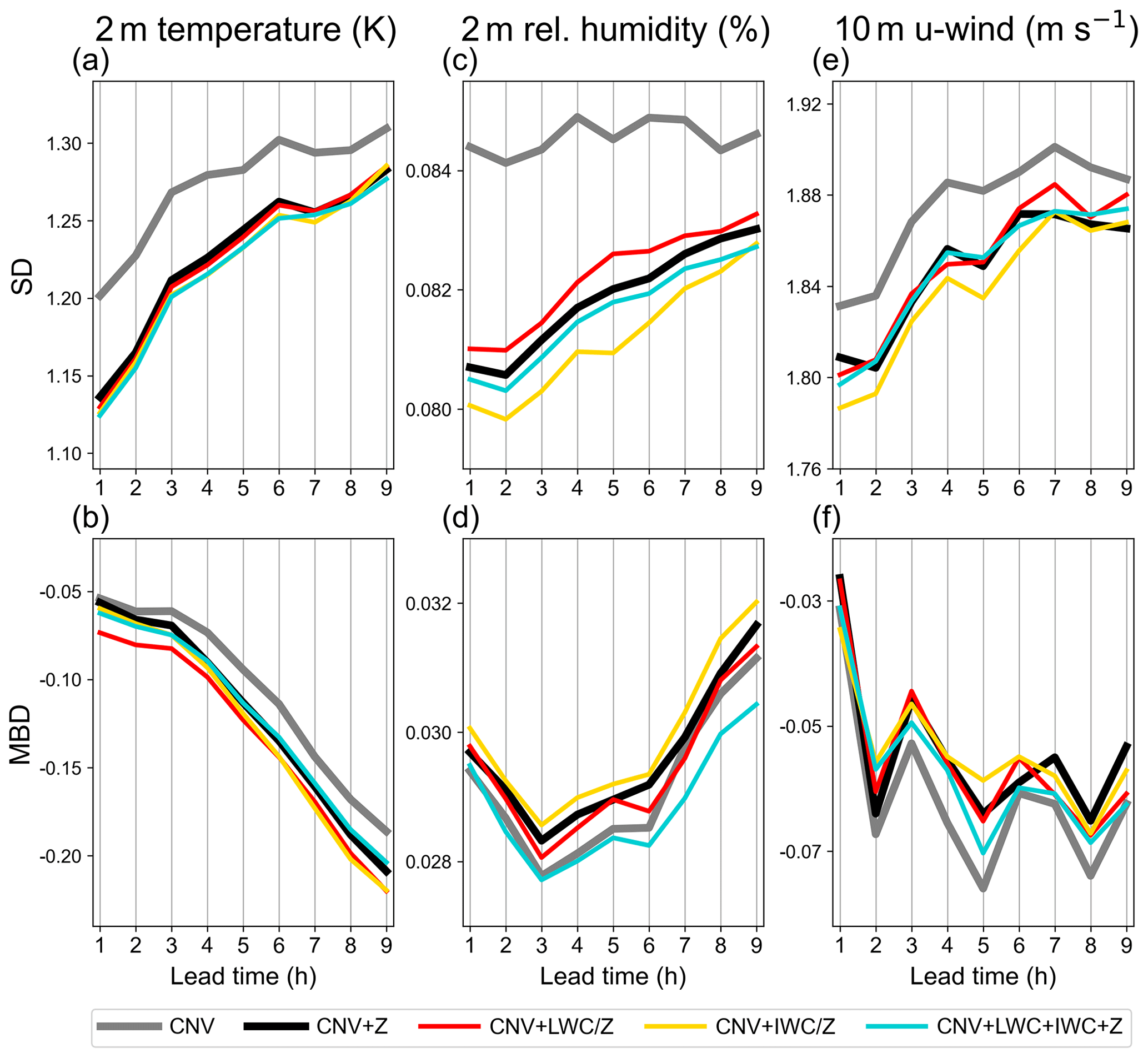
Figure 10 Mean standard deviations (SD; a, c, e) and mean bias deviations (MBD; b, d, f) of forecasted 2 m temperature (a, b), 2 m relative humidity (c, d), and 10 m u-wind (e, f) from conventional observations in Germany as functions of the forecast lead time. Means are calculated over 9 h forecasts initiated every third hour from hourly assimilation cycles with the assimilation configurations CNV (gray curves), CNV + Z (black curves), CNV + LWC$/Z$ (red curves), CNV + IWC$/Z$ (yellow curves), and CNV + LWC + IWC + Z (blue curves) using the best DAP settings found for the LWC and IWC assimilations (S2-06 and S1-02 in Table 2) in terms of first-guess QPF quality, and taking all rainfall cases C2017, S2017, and S2021 into account.

6 Conclusions

We assimilated for the first time polarimetric information from radar observations of the German C-band radar network in the KENDA-ICON-D2 system of DWD. In this study, we used microphysical retrievals of liquid and ice water content (LWC and IWC) and evaluated their impact on short-term precipitation forecasts. First, the impact of assimilating the microphysical retrievals on the first-guess (hourly) precipitation forecasts was investigated with different data assimilation parameter (DAP; e.g., observation localization length-scales and errors) sets and radar data set configurations. Then, the most successful assimilation settings were used to initiate 9 h precipitation forecasts.

Four data set configurations were analyzed to find the best DAP sets: only conventional observations (CNV), conventional and 3D reflectivity Z observations (CNV + Z), conventional data and 3D LWC estimates replacing Z observations where available (CNV + LWC$/Z$), and conventional data and 3D IWC estimates replacing Z observations where possible (CNV + IWC$/Z$). For the two stratiform cases in the summers of 2017 and 2021 and the one convective case in the summer of 2017, a rather small horizontal observation localization length-scale of 8 km and a lower limit of −1.15 in log ₁₀(LWC) and log ₁₀(IWC) yielded the best deterministic and ensemble first guesses. Thus, the best first guess of precipitation forecasts is achieved when the influence of the observed microphysical estimates on the model state is rather small in terms of observation localization length-scale and lower data limit. A rather small observation error standard deviation of 0.25 in log ₁₀(LWC) and log ₁₀(IWC) was most successful. The best values for the other DAPs differed for LWC and IWC: vertical localization length-scales were 0.2 in logarithm of pressure for LWC and 0.5 in the logarithm of pressure for IWC; best superobbing window sizes were 20 km for LWC and 10 km for IWC; the minimum number of valid values in the superobbing window was three observations for LWC and 50 % valid values for IWC.

The LWC assimilation (CNV + LWC$/Z$) with the best performing DAP setting with respect to the first-guess QPF quality improved the first guesses for most precipitation cases and accumulation thresholds compared with the CNV + Z configuration, whereas the best-performing DAP setting for IWC worsened the results, especially for the 2017 convective case, except for the stratiform case in 2021. The latter may be due to the radial resolution increase in the DWD volume scans from 1 km to 0.25 km in spring 2021. The higher resolution improves the specific differential phase K_DP estimation as part of the hybrid IWC retrieval, because more successive radar bins can be used for a given K_DP window size. One reason for the poor performance of the IWC assimilation, especially for the 2017 convective case, besides possible deficiencies in the model's ice module, may be the fact that the IWC retrieval was developed for snowfall but not for hail or graupel likely being present during intense convective summer precipitation in Germany. Interestingly, the LWC assimilation led to consistent improvements for convective situations, despite a retrieval not adapted to hail or graupel either. The application of a higher co-polar cross-correlation coefficient ρ_HV threshold below the melting layer for filtering may have masked radar pixels contaminated with hail or graupel.

In general, the best first-guess precipitation forecasts were obtained when all radar data sets (i.e., Z, LWC, and IWC) were assimilated together (CNV + LWC + IWC + Z).

9 h forecasts initiated with the CNV + LWC$/Z$ configuration using the best DAP setting with respect to first-guess QPF quality slightly outperformed the CNV + Z configuration in terms of deterministic FSS on average and for most forecast lead times with the best results for the 2017 convective case. The same applies to the assimilation of IWC (CNV + IWC$/Z$); however, the mean FSS mostly deteriorated for the convective case compared with the CNV + Z configuration, but was systematically improved over most of the forecast time for the high-resolution 2021 stratiform case. Forecasts initiated with the assimilation of all radar data sets (CNV + LWC + IWC + Z) yielded the best overall FSS. Furthermore, the assimilation of the LWC and/or IWC estimates (CNV + LWC$/Z$, CNV + IWC$/Z$, and CNV + LWC + IWC + Z) generally improved the mean frequency bias FBI over the CNV + Z configuration for most forecast hours.

We used DWD's standard configuration of KENDA, which only produces microphysical analysis increments in cloud water mixing ratio and specific humidity, i.e., not all available hydrometeor species (e.g., rain, cloud ice, and graupel mixing ratios) are updated individually. This setting was chosen at DWD to optimize the assimilation impact of Z (Klaus Stephan, DWD, personal communication, 2023). Thus, it remains to be explored how changes in the updated (microphysical) variables change precipitation forecasts when polarimetric information contained in microphysical retrievals is assimilated. For example, it should be investigated if the update of the rain mixing ratio via cross-correlations in the first-guess ensemble from LWC observation increments or the update of ice species (e.g., snow and/or cloud-ice mixing ratios) via cross-correlations from IWC innovations would yield improved forecasts.

Our study presented the benefits from the assimilation of state-of-the-art polarimetric microphysical retrievals below and above the melting layer adjusted for pure rain and snowfall respectively in a convective-scale NWP system in Germany. The results revealed only limited benefits with the assimilation of IWC retrievals in convective precipitation. As the retrievals are based on assumptions valid for snow but not for graupel or hail, e.g., the inversely proportional relationship between the density and size of the hydrometeors, the potential presence of graupel and/or hail in convection may be at least partly responsible. Accordingly, the development of more adequate retrieval algorithms for convective cores constitutes one of the next steps in further improving the exploitation of ice microphysical retrievals for radar data assimilation.