the Creative Commons Attribution 4.0 License.
the Creative Commons Attribution 4.0 License.
 | 26 Jan 2023
Modeling of street-scale pollutant dispersion by coupled simulation of chemical reaction, aerosol dynamics, and CFD
Chao Lin
Yunyi Wang
Ryozo Ooka
Cédric Flageul
Youngseob Kim
Hideki Kikumoto
Zhizhao Wang
Karine Sartelet
In the urban environment, gas and particles impose adverse impacts on the health of pedestrians. The conventional computational fluid dynamics (CFD) methods that regard pollutants as passive scalars cannot reproduce the formation of secondary pollutants and lead to uncertain prediction. In this study, SSH-aerosol, a modular box model that simulates the evolution of gas, primary and secondary aerosols, is coupled with the CFD software, OpenFOAM and Code_Saturne. The transient dispersion of pollutants emitted from traffic in a street canyon is simulated using the unsteady Reynolds-averaged Navier–Stokes equations (RANS) model. The simulated concentrations of NO2, PM10, and black carbon (BC) are compared with field measurements on a street of Greater Paris. The simulated NO2 and PM10 concentrations based on the coupled model achieved better agreement with measurement data than the conventional CFD simulation. Meanwhile, the black carbon concentration is underestimated, probably partly because of the underestimation of non-exhaust emissions (tire and road wear). Aerosol dynamics lead to a large increase of ammonium nitrate and anthropogenic organic compounds from precursor gas emitted in the street canyon.
- Article
(7653 KB) - Full-text XML
- BibTeX
- EndNote


Traffic-related pollutants can impose adverse effects on pedestrians' health in the urban environment (Anenberg et al., 2017; Jones et al., 2008). Especially particulate matter (PM) is strongly associated with increased cardiovascular diseases (Du et al., 2016). Therefore, investigating the dispersion of PM and the corresponding precursor gas is of great significance to evaluate the environmental impact and devise suitable countermeasures (Kumar et al., 2008).
With the development of numerical simulations, computational fluid dynamics (CFD) has been widely used for near-field dispersion prediction (Tominaga and Stathopoulos, 2013). The pollutant dispersion patterns in complex geometric and non-uniform building configurations can be well predicted using CFD simulations (Blocken et al., 2013). Pollutant dispersion, deposition and transformation (chemical reactions and aerosol dynamics) have primary roles in near-field prediction models. However, most CFD-based studies assume that the timescale of transport at the street scale (∼ 100 m) is relatively shorter than the timescale of deposition and transformation; therefore, they frequently regard pollutants as inert matter. Meanwhile, the recirculation flows which commonly exist in street canyons lead to low-ventilation zones and may provide sufficient time for transformation (Lo and Ngan, 2017; Zhang et al., 2020).
In addition, when PM is transported as a passive scalar, the distribution of the total concentration can be simulated; however, information on the particle size distribution and chemical composition is unclear. Understanding the size distribution is important for evaluating the health hazards because large particles are deposited in the mouth and upper airways, whereas smaller particles deposit deeper in the lungs and can even reach the alveolar region of the lungs (Sung et al., 2007). Moreover, as particles of different chemical compositions are related to different sources and/or precursor gases, gaining knowledge of their composition may help to devise countermeasures to limit their concentrations (Kim, 2019).
To simulate pollutant concentrations considering both transport and transformation, many studies have coupled air-quality models with gas-phase chemistry and aerosol modules and achieved chemical transport from a regional scale (∼ 100 km) (Sartelet et al., 2007) to a street scale (Lugon et al., 2021b). However, few models can simultaneously represent detailed particle dispersion in a complicated urban flow field considering secondary aerosol formation.
For the recent development and application of the CFD–chemistry coupling model, Kurppa et al. (2019) implemented a sectional aerosol module into large eddy simulation (LES) and conducted a particle dispersion simulation on a neighborhood scale. Gao et al. (2022) employed the same model to examine the dispersion of cooking-generated aerosols in an urban street canyon. In both studies, the effect of particle dynamics on aerosol number concentration was well reproduced. However, the simulated chemical composition was not detailed. In addition, the chemical reactions of the precursor gas were not considered. Kim et al. (2019) coupled the unsteady Reynolds-averaged Navier–Stokes equations (RANS) model with gas chemistry and aerosol modules and conducted simulations of PM1 in a street canyon under summer and winter conditions. The diurnal variations, spatial distribution, and chemical composition of pollutants in the street canyon were investigated. However, the size distribution of particles and the secondary organic aerosol (SOA) chemistry were not considered. Therefore, a more comprehensive coupled model is needed to simulate the evolution of gas concentrations, mass, and number concentrations of primary and secondary particles at the same time.
Vehicles are considered to be the main ammonia (NH3) source in urban environments (Sun et al., 2017). Reactive nitrogen emissions from many new vehicles are now dominated by NH3 (Bishop and Stedman, 2015). Since the formation of ammonium nitrate is often limited by HNO3 rather than NH3 in urban areas (NH3-limited), increasing NH3 may lead to increased ammonium nitrate production and PM concentration in urban streets (Lugon et al., 2021b). However, NH3 emissions from passenger cars are usually not regulated (Suarez-Bertoa and Astorga, 2018). Therefore, to provide evidence in making policies for NH3 emission regulation, it is important to investigate the local influence of NH3 emissions on PM concentrations.
Therefore, to achieve a more comprehensive simulation of PM and related precursor gas, this study couples software of two open-source CFD: OpenFOAM (OpenFOAM user guide) and Code_Saturne (Archambeau et al., 2004), with gas-phase chemistry and aerosol module SSH-aerosol (Sartelet et al., 2020). Both OpenFOAM and Code_Saturne own wide users. Therefore, coupling SSH-aerosol with software of both CFD may satisfy more needs. Simulations of the PM concentrations in a 2-D street canyon are conducted. The coupled model is validated by comparison to field measurements. The size distributions and chemical compositions of particles from the models with and without secondary aerosol formation are compared. In addition, cases with large NH3 emissions are considered and the related PM increase is investigated.
The remainder of this paper is organized as follows. The coupling of the aerosol model and CFD is introduced in Sect. 2. The computational details are presented in Sect. 3. In Sect. 4, the simulated pollutant concentrations are compared with field measurements, followed by evaluations of the influence of the grid, coupling method, and time step. In Sect. 5, spatial and temporal variations in the concentrations are analyzed. The chemical compositions and size distributions of the particles between the coupled model and the model that does not consider gas chemistry or aerosol dynamics are compared. In addition, the effect of NH3 traffic emissions on particle concentrations is discussed. Finally, the conclusions and perspectives are presented in Sect. 6.
The coupling method between CFD and chemistry modules is similar to the literature (Gao et al., 2022; Kurppa et al., 2019). OpenFOAM v2012 and Code_Saturne 6.2 are used to solve the governing equations of the flow field and transport equations of gas and particle mass fractions. The inflow conditions, pollutants' background concentrations, and emission rates are obtained from regional models and are linearly interpolated into each time step; this will be introduced in Sect. 3. This simulation method is called the transient-condition method (TCM) in this study. However, because time-varying flow fields and concentration fields are expensive to compute in terms of computational time, conducting CFD simulations with fixed boundary conditions and emission rates at specific time points is considered a practical method for evaluating street-level pollutant concentrations (Wu et al., 2021; Zhang et al., 2020). The transport (advection and diffusion) and chemical processes will reach equilibrium, and the simulated concentrations will reach quasi-stable values. These values are often regarded as time-averaged concentrations. This method is called the constant-condition method (CCM) in this study, in contrast to TCM. However, the simulation accuracy of CCM has not been validated in simulations that consider both gas chemistry and particle dynamics. Therefore, validation is conducted using boundary conditions and emission rates at specific time points and the simulated concentrations with CCM and TCM are compared in Sect. 4.2.
The unsteady RANS model is used for the transient simulations with both CFD codes. In OpenFOAM, the RNG (re-normalization group) k–ε model (Yakhot et al., 1992) is deployed for turbulence closure. All transport equations are discretized using the total variation diminishing (TVD) scheme (Harten, 1984; Yee, 1987), which combines the first-order upwind difference scheme and the second-order central difference scheme. The PIMPLE algorithm, a merged PISO (Pressure Implicit with Splitting of Operator) – SIMPLE (Semi-Implicit Method for Pressure-Linked Equations) algorithm in the OpenFOAM toolkit, is used for pressure–velocity coupling. In Code_Saturne, turbulence is solved using the k–ε turbulence model (linear production) (Guimet and Laurence, 2002). The time and space discretization of velocity, pressure, and other scalars in all transport equations are realized through a centered scheme and a fractional step scheme (Archambeau et al., 2004). For both CFD software, the dry deposition schemes for gas and particle are added to the transport equations using volume sink terms based on Zhang et al. (2003) and Zhang et al. (2001), respectively. The details of the implementation are provided in Appendix A.
The SSH-aerosol (Sartelet et al., 2020) is a modular box model that simulates the evolution of not only gas concentrations but also the mass and number concentrations of primary and secondary particles. In SSH-aerosol, 112 gas species and 40 particle species are considered. The particle compounds are dust, black carbon (BC), inorganics (sodium, sulfate, ammonium, nitrate, and chloride), primary organic aerosol (POA) and secondary organic aerosol (SOA). Three main processes involved in aerosol dynamics (coagulation, condensation/evaporation, and nucleation) are included. The particle size distribution is modeled using a sectional size distribution. Nucleation is not considered in this study because only the mass and not the number of particles is available for evaluation, and large uncertainties remain on the nucleation parameterizations (Sartelet et al., 2022) that mostly affect the number of particles. As nucleation is not considered, the minimum diameter does not need to be as low as 0.001 µm, and it is fixed to 0.01 µm, as in the regional-scale simulations of Sartelet et al. (2018), which provide the background concentrations. Six particle size sections are employed with bound diameters of 0.01, 0.04, 0.16, 0.4, 1.0, 2.5, and 10 µm.
The coupling between CFD and SSH-aerosol is achieved by using the application program interface (API) of SSH-aerosol. The gas and particle concentrations are initialized in CFD and transported in the domain for each time step. For each grid volume cell, these transported concentrations, as well as meteorological parameters, such as temperature and humidity, are then sent to SSH-aerosol to advance 1 time step of gaseous chemistry and aerosol dynamics. Once the SSH-aerosol calculation is completed, the concentrations are sent back to the CFD for the next time step. It should be noted that as the SSH-aerosol processes the ensemble-averaged concentration from the RANS model, the covariance of turbulent diffusion and chemical reaction may not be fully reproduced. The influence of different operator splitting algorithms is discussed in Sect. 4.4.
The simulation is set up to model a street in Greater Paris (Boulevard Alsace-Lorraine), where field measurements were conducted from 6 April to 15 June 2014. The concentrations of nitrogen dioxide (NO2), particles with diameters less than 10 µm (PM10), and black carbon were measured as described in Kim et al. (2018). Figure 1 shows the simulation domain. The 2-D street canyon is 27.5 m in width (W) and 8.5 m in height (H). The domain height is 6 H. The street canyon is discretized into uniform grids in x and z directions. The grid resolutions in the street canyon are 0.5 m in both x and z directions, respectively. The largest grid sizes are 4 m (x) × 2 m (z). An analysis of the grid sensitivity is described in Sect. 4.3.

Simulations are conducted from 04:30 LT to 17:00 LT on 30 April 2014 at local time (GMT+2). This period is selected because the wind direction is almost perpendicular to the street canyon during that day, allowing for a 2-D simulation setting. During the field measurement, there are several time periods when the wind direction is perpendicular with the street canyon. Meanwhile, some time periods are short (less than 5 h), and we consider that such a short period simulation is not representative in simulation accuracy. In addition, we consider that it is critical to have a simulation time long enough to cover both daytime chemistry and nighttime chemistry. The first 30 min of the simulation corresponds to model spin-up, and the simulation lasts 12 h. A sensitivity analysis of numerical aspects, such as the splitting method between transport and chemistry and the time step, is described in Sect. 4.4.
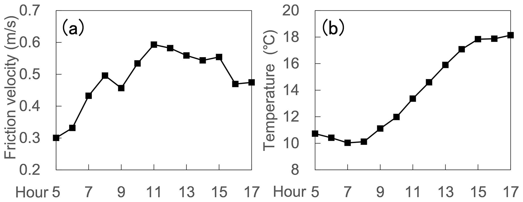
Meteorological conditions (Fig. 2) including time-varying friction velocity and temperature are obtained from the simulation described in Sartelet et al. (2018) using the Weather Research and Forecasting (WRF) model. The grid resolution is 1 km × 1 km in Paris. The lowest and highest friction velocities occurred approximately at 05:00 LT and 11:00 LT, respectively. The lowest and highest temperatures are around 08:00 LT and 17:00 LT. For the inflow, the wind direction is perpendicular to the street canyon. The friction velocity u∗ is used to prescribe the vertical profiles of the streamwise velocity U, turbulent kinetic energy k, and turbulent dissipation rate ε as follows:
where κ is the von Kármán constant and Cμ is the model constant (=0.09) in the k–ε model. The roughness length z0 is set to 1 m for the inlet (Belcher, 2005) and 0.1 m for the wall and bottom (Lo and Ngan, 2015).
In addition, since the domain height is low (51 m) in this study and we focus on the pollutant dispersion behaviors in the street canyon, it is reasonable to consider the atmospheric stability as neutral; therefore, the temperature is assumed to be spatially uniform at the inflow. The hourly friction velocities and temperatures are linearly interpolated into each time step and prescribed at the inflow. It should be noted that the general trends are simulated but the fast fluctuations at the inlet are not reproduced. The same linear interpolation is used for background concentrations and emission rates, which will be described in the following.
Figure 3a shows the time variations of the PM10, NO, and NO2 background concentrations. Figure 3b and c show the emission rates for NO, NO2, and the emitted compounds of PM10. The background concentrations of the gas and particles are obtained from the regional-scale simulations of Sartelet et al. (2018) with the Eulerian model Polair3D of the Polyphemus air quality modeling platform (Mallet et al., 2007) which uses the same chemical representation as in this study. As detailed in Sartelet et al. (2018), the regional background concentrations compare well to measurements of O3, NO2, PM10, PM2.5, black carbon, and organic aerosols. The hourly background concentrations are linearly interpolated into each time step, and the spatial distribution is uniformly prescribed at the inflow and top. The traffic emission source is assumed to be approximately 14 m in width and 1.5 m in height, and it is set in the middle of the bottom of the canyon (Fig. 1). As detailed in Kim et al. (2022), emissions are estimated from the fleet composition and the number of vehicles in the street using COPERT's emission factors (COmputer Program to calculate Emissions from Road Transport, version 2019, EMEP/EEA, 2019). After the speciation of NOx, volatile organic compounds (VOCs), PM2.5, and PM10 into model species, emissions are set for 16 gaseous model species and 3 particle model species: dust and unspecified matter (dust), black carbon (BC), and primary organic aerosol of low volatility (POAlP). The PM size distribution at emission is assumed to be the same as in the previous studies (Lugon et al., 2021a, b). The exhaust primary PM is assumed to be in the size bin (0.04–0.16 µm)while non-exhaust primary PM is coarser in the size bin (0.4–10 µm).
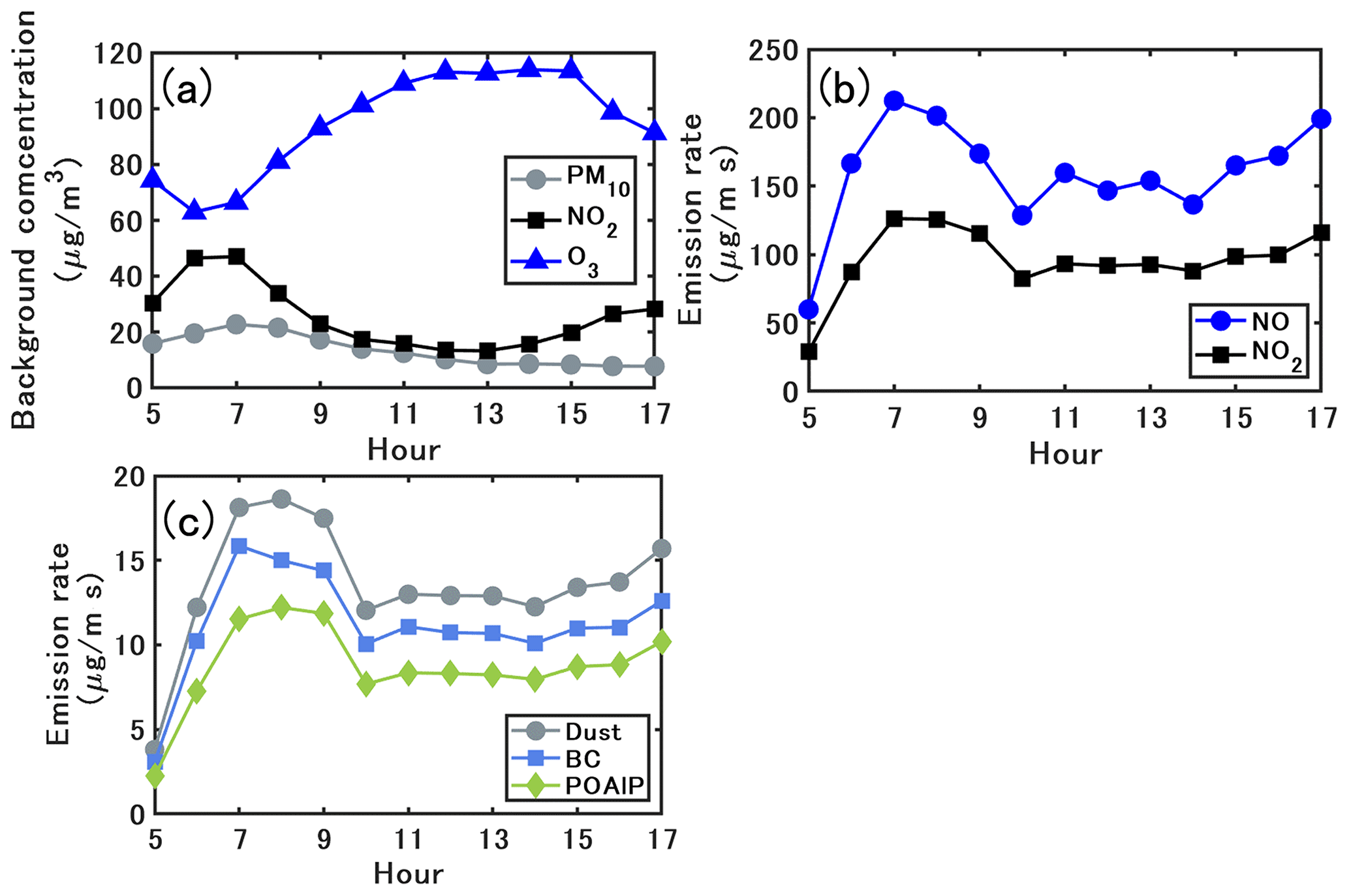
Figure 3Time variations of (a) PM10, NO and NO2 background concentrations, (b) emission rates of NO and NO2 and (c) emission rates of dust, BC, and organics (POAlP).
For the boundary conditions of OpenFOAM, the pressure and gradients of all other variables are set to zero at the outlet. For the walls, we use the wall functions of ε and turbulent kinematic viscosity νt for atmospheric boundary layer modeling in the OpenFOAM toolkit (OpenFOAM user guide) based on Parente et al. (2011). The gradients of turbulent kinetic energy k, concentration, and temperature are set to zero. In Code_Saturne, a two-scale logarithmic friction velocity wall function is used for solving the fluid velocity near wall cell and a three-layer wall function is used for computing other transported scalar profiles such as temperature near the wall (Arpaci and Larsen, 1984).
The turbulent Schmidt number Sct in the concentration transport equations, which is the ratio of the turbulent diffusivity to the concentration and turbulent kinematic viscosity, is important in turbulent diffusion modeling. The value of Sct is considered between 0.2 and 1.3, depending on the flow properties and geometries (Tominaga and Stathopoulos, 2007). For urban environments with a compact layout, a small Sct=0.4 is found to show better agreement with wind tunnel experiment data (Di Sabatino et al., 2007). Therefore, a value of 0.4 is adopted in the current study.
4.1 Validation with field measurements and comparison of simulated concentrations with the two CFD software
Reproducing the flow field is important in this study. Meanwhile, the observation data on wind velocity are not available. Therefore, we conducted a velocity validation for OpenFOAM v2012 using data from a wind tunnel experiment (Blackman et al., 2015). The predicted mean velocity agreed well with the experimental values. The details can be found in Appendix B.
Figure 4 compares the simulated concentrations with those obtained from the field measurements. In the field measurements, the measured concentration was obtained from averaging over two measurement points near the leeward and windward walls in the street canyon. In this section, the simulated results and discussion are based on the spatially averaged values in the street canyon . The CFD–passive and CFD–chemistry denote the CFD simulation without and with chemistry coupling, respectively. The OF and CS denote simulated concentrations based on OpenFOAM and Code_Saturne, respectively. The operator splitting order and time step for OF and CS are the A-B-A splitting method with 0.5 s and the A-B splitting method with 0.25 s, as detailed in Sect. 4.4. The simulation time ratio of CFD–chemistry and CFD–passive is about 3 times in both OpenFOAM and Code_Saturne in this study.
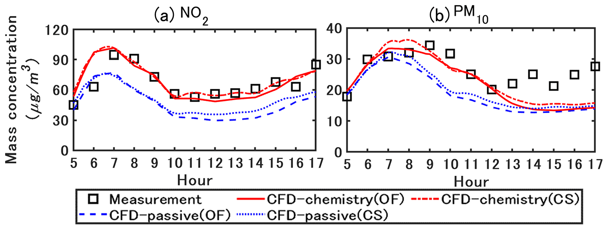
Figure 4Measured and simulated NO2 and PM10 concentrations. The values are spatially averaged in the street canyon . CFD–passive and CFD-chemistry denote the CFD simulation without and with chemistry coupling, respectively. OF and CS denote the simulated concentrations based on OpenFOAM and Code_Saturne, respectively. All concentrations are represented in local time (GMT+2).
For NO2, the peak concentration in the field measurement occurred approximately at 07:00 LT owing to the morning traffic. In the CFD–passive simulations, the lack of chemical reactions lead to an underestimation of NO2, while the concentrations simulated with CFD–chemistry agree well with the measurements. For PM10, the concentrations simulated with CFD–chemistry also show better agreement with the measurements than CFD–passive. The primary reason is that CFD–chemistry can reproduce the condensation of inorganic and organic matter from the gas phase to the particle phase, which will be further explained in the following sections. The simulation results based on OF and CS show small differences, and detailed comparisons are presented in Fig. 6.
Validation metrics (Chang and Hanna, 2004) are used to quantify the overall accuracy of the CFD simulated concentrations based on OF compared with the measured values (Trini Castelli et al., 2018; Ferrero et al., 2019). The following metrics are used: fractional bias (FB), geometric mean bias (MG), and normalized mean square error (NMSE). These metrics are defined as follows:
where Obsi and CFDi are the measured and CFD-simulated concentrations for the compound/species i, respectively. The overbar represents the mean value of the entire dataset. The ideal values are 1 for MG and 0 for FB and NMSE. Previous research has suggested that are acceptable for simulated concentrations (Hanna et al., 2004).
Table 1 shows the statistical indicators for spatially averaged concentrations of NO2 and PM10 in the street canyon from 05:00 LT to 17:00 LT. For NO2 and PM10, the mean and 90 % percentile concentrations simulated with CFD–chemistry are closer to the measurements than those simulated with CFD–passive. In addition, the FB, MG, and NMSE values of CFD–chemistry are closer to the ideal values than those of CFD–passive.
Table 1Statistical indicators for NO2 and PM10 in the street canyon from 05:00 LT to 17:00 LT. The concentrations are simulated with OpenFOAM.

The black carbon (BC) concentration simulated with OF is compared with the measurements in Fig. 5. Because BC is considered an inert matter, considering chemistry does not influence the mass concentration. Therefore, the concentrations simulated with CFD–passive and CFD–chemistry show little difference; only the concentration simulated with CFD–chemistry is shown here. The BC concentrations are underestimated by a factor of approximately 5. Even the maximum concentrations in the street canyon largely underestimate the measurements. One of the causes of this underestimation may be the underestimation of the non-exhaust tire emission factors in the COPERT emission factors used here (Lugon et al., 2021a).
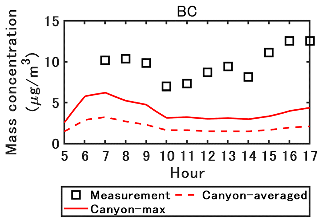
Figure 5Measured and simulated black carbon concentrations with OpenFOAM. The canyon-averaged and maximum concentrations in the street canyon are represented by the plain line and the dashed line, respectively .
The particle concentrations simulated with OF and CS are compared in Fig. 6. The evolutions of the concentrations simulated by OF and CS are similar. Higher PM10 concentrations are simulated by CS around 08:00 LT during the traffic peak and in the afternoon, mostly because of the higher concentrations of emitted inert compounds such as black carbon and dust. Differences in the turbulence scheme may explain these variations. Meanwhile, the difference between CFD–passive and CFD–chemistry for the inorganic and organic matter is in accordance with OF and CS, showing the robustness of the coupling method between CFD and SSH-aerosol by API. For simplicity, only the simulated concentration based on OF is presented and discussed in the following sections.

Figure 6Simulated particle concentrations with OpenFOAM (OF) and Code_Saturne (CS). CFD–passive and CFD–chemistry denote the CFD simulation without and with chemistry coupling, respectively.
4.2 Transient-condition method and constant-condition method
To validate the simulation accuracy of CCM in simulations that consider both gas chemistry and particle dynamics, simulations are conducted using boundary conditions and emission rates at five time points (07:00 LT, 10:00 LT, 13:00 LT, 15:00 LT, and 17:00 LT). Other simulation conditions, including the grid, coupling method, and time step, are the same as the transient-condition simulation.
In Fig. 7, for PM10 and NO2, the concentrations simulated with CCM (red triangles) are similar to those simulated with TCM. In addition, depending on the background concentration and emission conditions, the simulation time required for CCM to reach dynamic equilibrium is less than 1000 time steps (approximately 500 s). Therefore, CCM can be utilized for parameter studies. The sensitivity analysis of the grid, coupling method, and time step in Sect. 4.3 and 4.4 is based on CCM. However, CCM should be used with caution when the inflow wind speed and direction vary rapidly. The simulated concentrations in Sect. 5 are based on TCM.
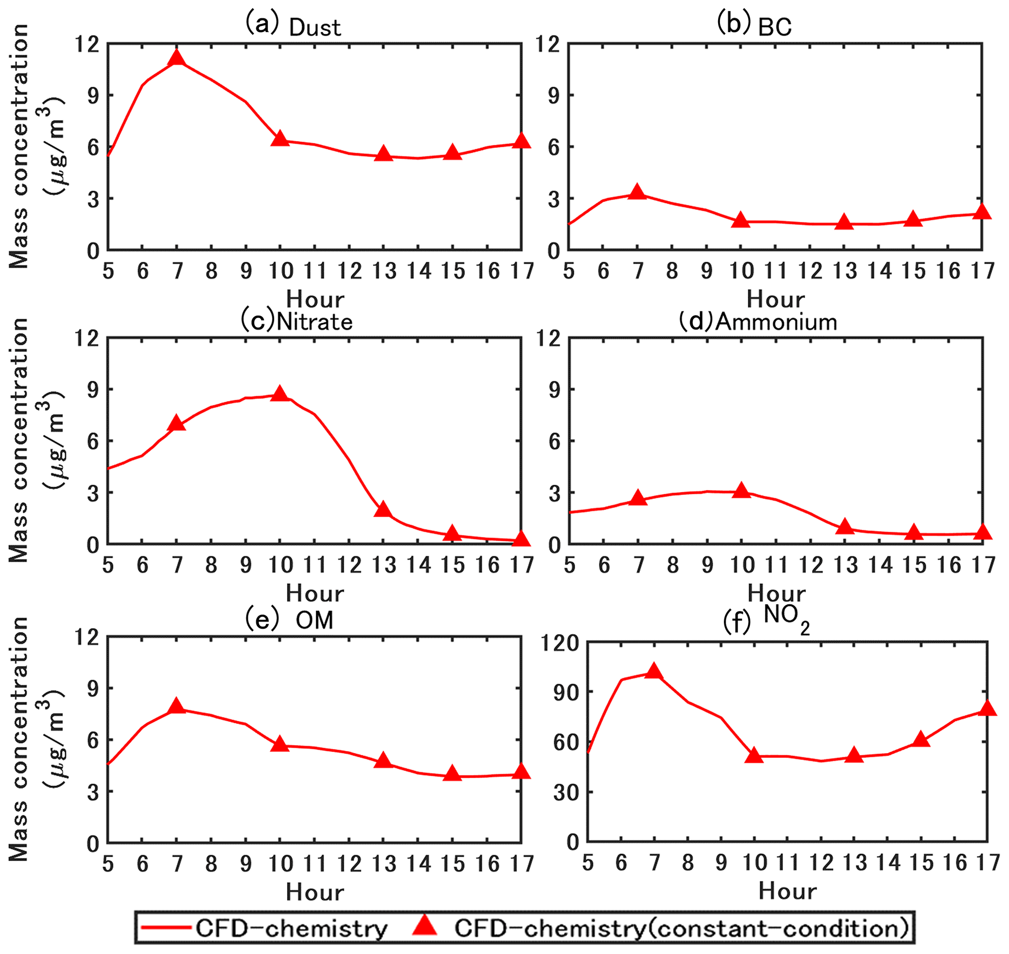
Figure 7Simulated PM10 and NO2 concentrations with the transient-condition and constant-condition methods. The concentrations are spatially averaged in the street canyon.
4.3 Grid sensitivity
A grid sensitivity analysis is conducted based on three different resolutions as shown in Fig. 8. The grid resolutions in the street canyon for coarse, basic, and fine grids are 1 m, 0.5 m, and 0.25 m in both x and z directions, respectively. The largest grid sizes are 4 m (x) × 2 m (z) for the coarse and basic grids, and 2 m (x) × 2 m (z) for the fine grid. The simulations are based on the constant-condition method (CTM). The A-B-A splitting method, which is introduced in Sect. 4.4, is used with a time step of 0.5 s. Figure 9 shows the comparative results for the mass concentration. No significant discrepancy is observed between the different grids for NO2, inert matter, and organic matter. Meanwhile, the simulated inorganic matter based on coarse grids shows slightly smaller concentrations than the other grid resolutions, while the concentrations based on basic and fine grids are close. Therefore, the basic grid is adopted for simulations in this study.
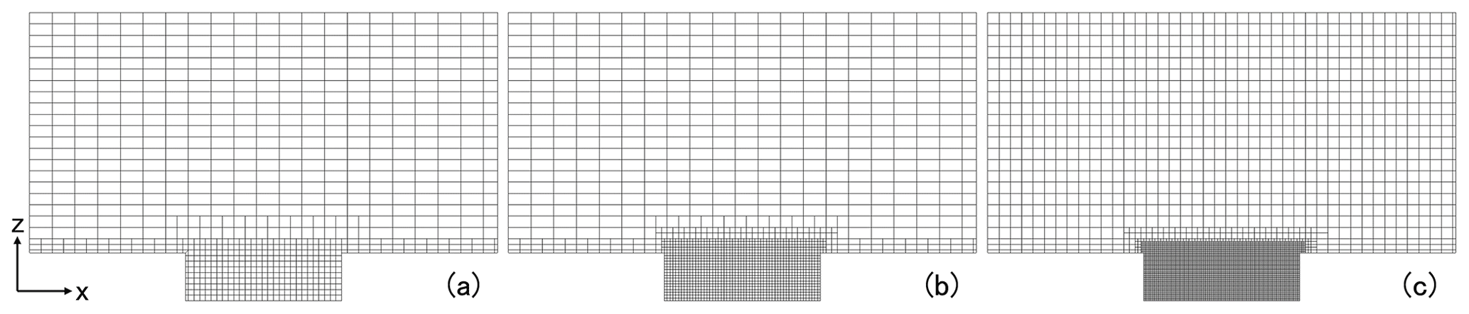
Figure 8Different grid resolutions for sensitivity analysis: (a) coarse, (b) basic, (c) fine. The grid resolutions in the street canyon are 1 m, 0.5 m, and 0.25 m in both x and z directions, respectively. The largest grid sizes are 4 m (x) × 2 m (z) in the coarse and basic grids, and 2 m (x) × 2 m (z) in the fine grid.

4.4 Coupling method and time step sensitivity
The transport equation for the chemical species includes terms of advection, diffusion, emission, and chemical reactions. Ideally, the transport equation should be solved with all the above terms, that is, by coupling all processes. However, the chemical process is integrated with a stiff integrator, whereas advection, diffusion, and emission are integrated with a flux scheme. Therefore, operator splitting (Sportisse, 2000) is often employed to solve different terms individually and sequentially over a given time step in chemical transport simulations (Fu and Liang, 2016).
In this study, advection, diffusion, and emission are simultaneously solved in CFD, and the chemical reactions including gas chemistry, particle dynamics, and size redistribution are solved in SSH-aerosol. Two operator-splitting orders are considered for coupling: A–B splitting and A–B–A splitting (Sportisse, 2000). For A-B splitting, which can be summarized as CFD(Δt)–Chemistry(Δt), the mass concentrations are first integrated for transport over a time step Δt. The updated concentrations are then integrated for chemistry at the same Δt. On the other side, A–B–A splitting adopts a symmetric sequence of operators, which can be summarized as CFD()–Chemistry(Δt)–CFD(). The mass concentrations are first integrated for transport over a half time step, then for chemistry over the full time step, and finally for transport again over a half time step.
Table 2Relative change in the computation time with different operator-splitting order and time steps. The computation time is normalized by ABA-05.
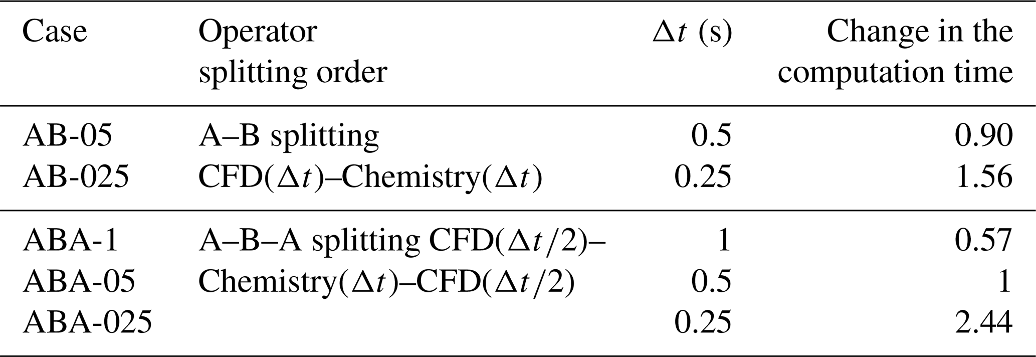
A sensitivity analysis is conducted on the operator-splitting method and splitting time step. As shown in Table 2, the time step is considered 0.5 and 0.25 s for the A–B splitting (named AB-05 and AB-025), and 1, 0.5, and 0.25 s for the A–B–A splitting (named ABA-1, ABA-05, and ABA-025). The simulated NO2 and particle concentrations are presented in Fig. 10. The ABA-1 and AB-05 concentrations hardly differ from the figures. Meanwhile, the computational time of ABA-1 is only 63 % of that of AB-05. Similarly, the concentrations simulated with ABA-05 and AB-025 are almost the same, and the computational time of ABA-05 is only 64 % of AB-025. Therefore, the A–B–A splitting method can be considered as a cost-effective method.

Figure 10Simulated NO2 and particle concentrations with different coupling methods and time steps. ABA denotes the A–B–A splitting method: CFD()–Chemistry(Δt)–CFD(). AB denotes the A–B splitting method: CFD(Δt)–Chemistry(Δt). In the legend, the values that follow the capital letter ABA or AB denote the time step Δt (in s) used in the simulation.
The concentrations simulated with the A–B–A splitting method and different time steps show that a small time step results in low inorganic and organic matter concentrations. The concentrations simulated with ABA-1 are larger than those of ABA-05, and larger than ABA-025. However, the differences between the concentrations simulated with ABA-05 and ABA-025 are lower than the differences between ABA-1 and ABA-05. For NO2 and inert particles, no obvious difference is found between the simulations with different splitting methods and splitting time steps. Therefore, the A–B–A splitting method with a time step of 0.5 s is adopted in this study.
5.1 Time-averaged flow field and concentration field
This section shows the results for time-averaged values from 05:00 LT to 17:00 LT. Figure 11 shows the 12 h time-averaged streamwise velocity and wind direction in the street canyon. At the current aspect ratio (), a large vortex is observed in the canyon with a small secondary vortex at the corner of the leeward wall. A reverse flow is observed in the lower half of the canyon.

Figure 12 shows the time-averaged concentrations of the gaseous pollutants from 05:00 LT to 17:00 LT. For gaseous pollutants emitted by traffic, such as NO2, NO, and NH3, larger concentrations are found in the street, particularly near the leeward wall, compared to the windward wall due to the reverse flow. Simultaneously, gas-phase chemistry and condensation/evaporation between the gas and particle phases also influence the concentration distribution. NO2 mainly increases due to chemical production from NO emissions and background O3. Compared to the background NO2 concentration of 26 µg m−3, the longest retention time at the leeward side corner leads to the street canyon's largest concentration (121 µg m−3). At pedestrian height (z=1.5 m), NO2 concentration is 116 µg m−3 at the leeward wall and 49 µg m−3 at the windward wall.
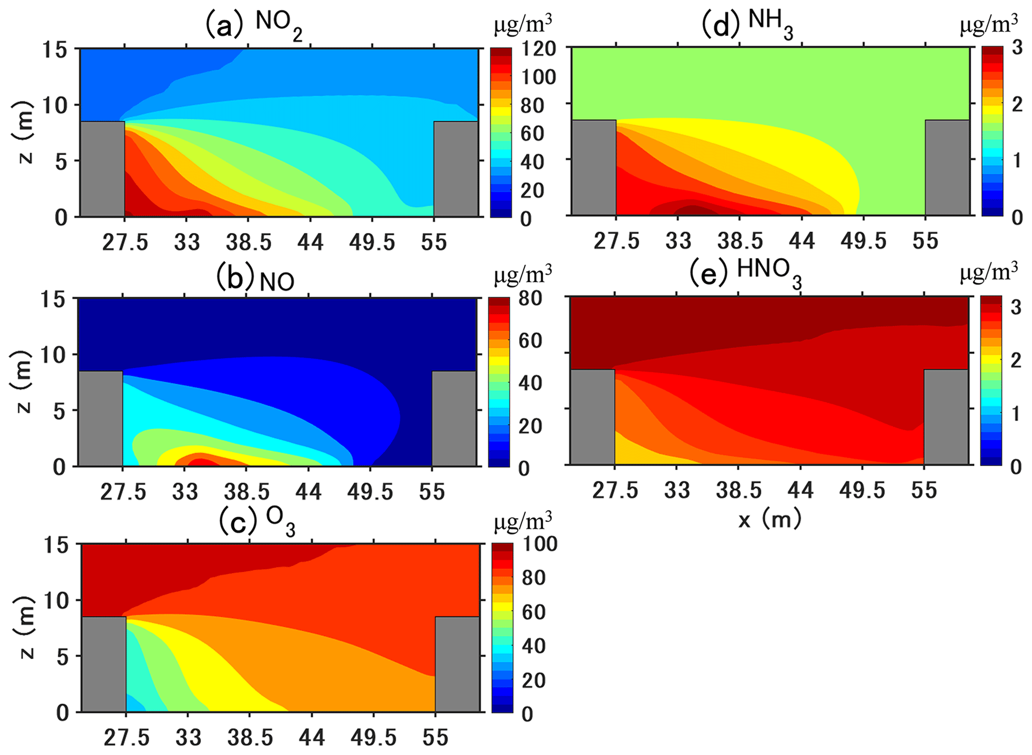
Figure 12Time-averaged concentrations (µg m−3) of gaseous pollutants in the street canyon from 05:00 LT to 17:00 LT.
However, NO and NH3 generally decrease because of loss by gaseous chemistry and the condensation of ammonium nitrate, respectively; therefore, the largest concentrations are at the leeward corner of the traffic emission source. For secondary gaseous pollutants without traffic emissions such as O3 and HNO3, gaseous chemistry and condensation lead to lower concentrations in the street canyon than background concentrations. For O3, this is due to the titration of O3 by NO, whose concentration is large near the leeward wall. For HNO3, this is because of the high concentrations of NH3, which then condenses with HNO3 to form ammonium nitrate. In addition, the lowest concentration of O3 and HNO3 can be found at the leeward corner which corresponds to the secondary vortex in Fig. 11, indicating that the pollutant residence time is the highest in that corner leading to enhanced ozone titration.
Figure 13 shows the time-averaged PM10 mass concentration and the number concentrations and PM composition (inorganic, organic and inert matter) from 05:00 LT to 17:00 LT. For inert and organic matter, the highest concentrations are near the leeward corner of the traffic emission source. Because inorganic matter is not emitted, the concentration distribution differs from inert and organic matter. However, as they are produced from gas condensation and strongly influenced by traffic emissions, the highest concentrations are observed in the leeward corner.
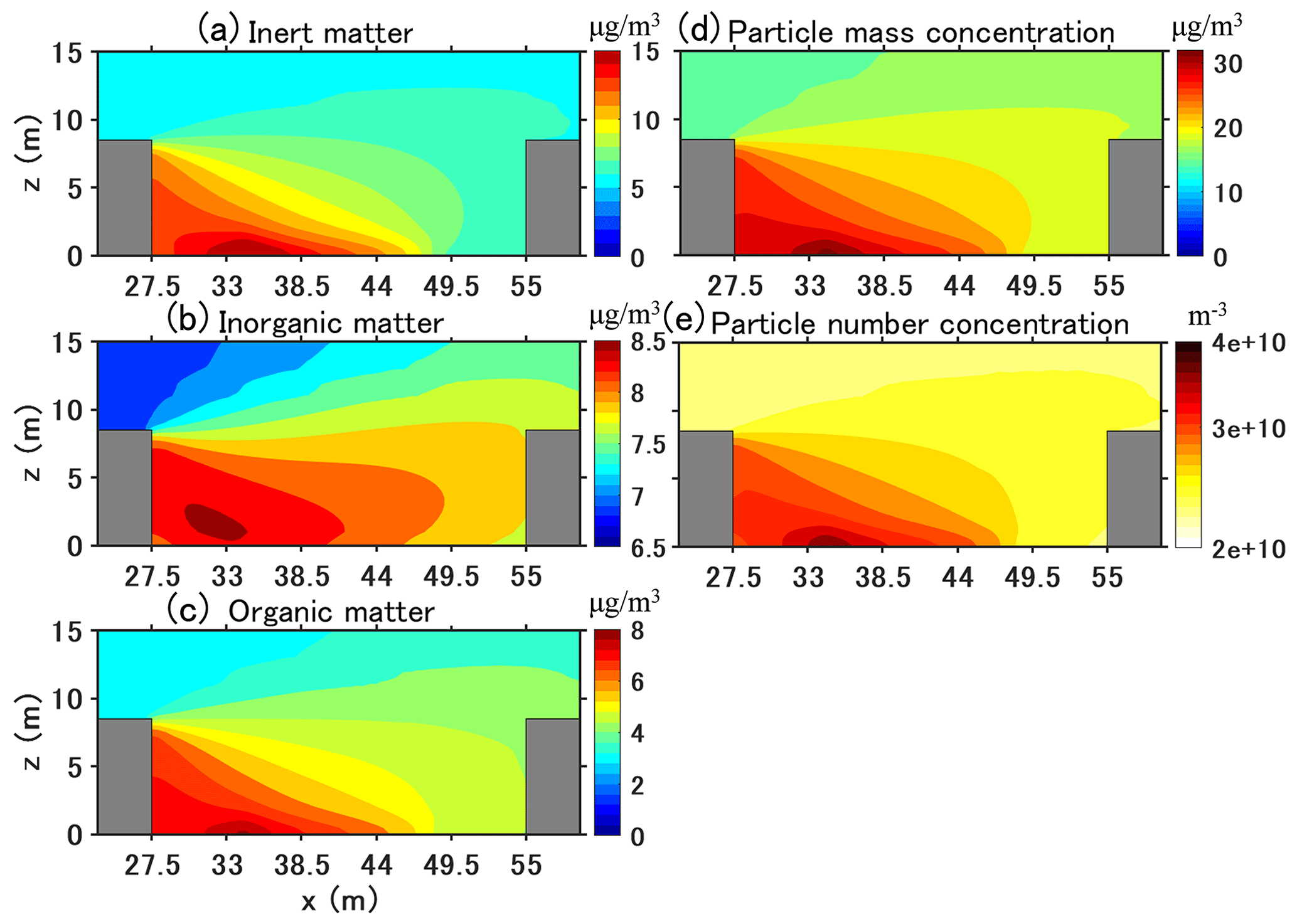
Figure 13Time-averaged concentrations of particle number, mass, and composition in the street canyon from 05:00 LT to 17:00 LT. The unit is µg m−3 for mass concentration and m−3 for number concentration.
At pedestrian height (z=1.5 m), the PM10 mass concentration is approximately 28 µg m−3 at the leeward wall and 19 µg m−3 at the windward wall, which is larger than the background concentration of 15 µg m−3. The number concentration is computed from the mass concentration and therefore has a similar spatial distribution as PM10 mass concentration (nucleation from gas was not taken into account). Traffic emission significantly increases the number concentration. The number concentration is about 2.3×10¹⁰ m−3 in the background, whereas the largest number concentration in the street canyon is about 3.8×10¹⁰ m−3.
5.2 Time-variant characteristics
Figure 14 shows the simulated time-varying concentrations of ammonium nitrate formed by the condensation of HNO3 and NH3. Based on the traffic fleet in the current study, NH3 emission is approximately 1 %–2 % of NOx emissions. Ammonium nitrate and HNO3 are not emitted and differences between simulations with or without chemistry coupling are due to gas chemical reactions and phase change between the gas and particle. Phase change may be driven by NH3 emissions as well as the non-thermodynamic equilibrium of the background concentrations.
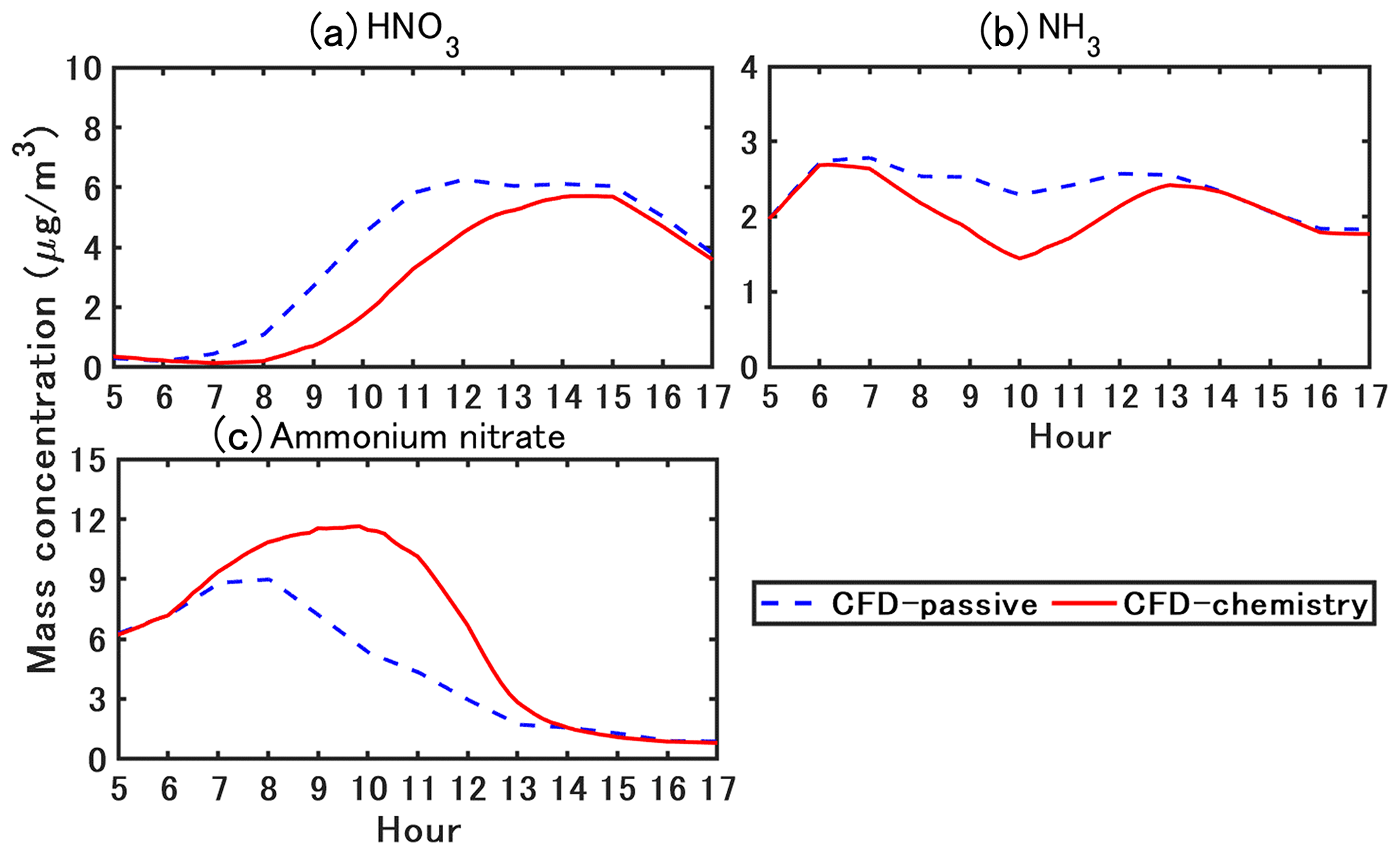
Figure 14Simulated time-varying concentrations of ammonium nitrate and precursor gas (HNO3 and NH3).
In CFD–passive, NH3 concentration peaks around 07:00 LT as NOx because it is emitted by traffic. The peak in HNO3 concentration is later in the morning, around 11:00 LT. HNO3 is formed from the oxidation of NO2, which is emitted by traffic and is rapidly formed from NO traffic emissions. The formation of HNO3 is slower than the formation of NO2; it probably occurs at the regional scale, leading to a delay in the peak of HNO3 concentration compared to NO2 concentration. In CFD–chemistry, the temporal variations of HNO3 concentration show large differences with CFD–passive because HNO3 condenses with NH3 to form ammonium nitrate during the daytime. As a result, the HNO3 concentration peak in CFD–chemistry is later than that in CFD–passive (it is shifted from 11:00 LT to around 14:00 LT). The NH3 concentration in CFD–passive peaks at 07:00 LT because of traffic emission and is stable from 07:00 LT to 13:00 LT and then decreases from 13:00 LT. Meanwhile, the condensation in CFD–chemistry leads to lower concentration than in CFD–passive during the daytime (between 07:00 LT and 13:00 LT).
For 12 h time-averaged concentrations, ammonium nitrate increases by 46 % in CFD–chemistry compared with that in CFD–passive. Background ammonium nitrate concentration (CFD–passive) peaks around the morning rush (07:00–08:00 LT) and then decreases. Meanwhile, in CFD–chemistry, ammonium nitrate concentration peaks later around 10:00 LT because of the large increase in HNO3 between the traffic rush and 10:00 LT. However, although HNO3 concentration does not vary much between 11:00 LT and 15:00 LT, the ammonium nitrate concentration decreases from 10:00 LT to a very small level (lower than 1 µg m−3) after 14:00 LT. This decrease is probably linked to the temperature increase during the daytime (Fig. 2b) and the relative humidity decrease, leading to a decrease in the condensation rate (Stelson and Seinfeld, 1982).
Figure 15 shows the simulated time-varying concentrations of organic matter. Organic matter is divided into two main categories depending on the origin of the precursors: Bio and Ant refer to the organic matter of biogenic and anthropogenic precursors, respectively.
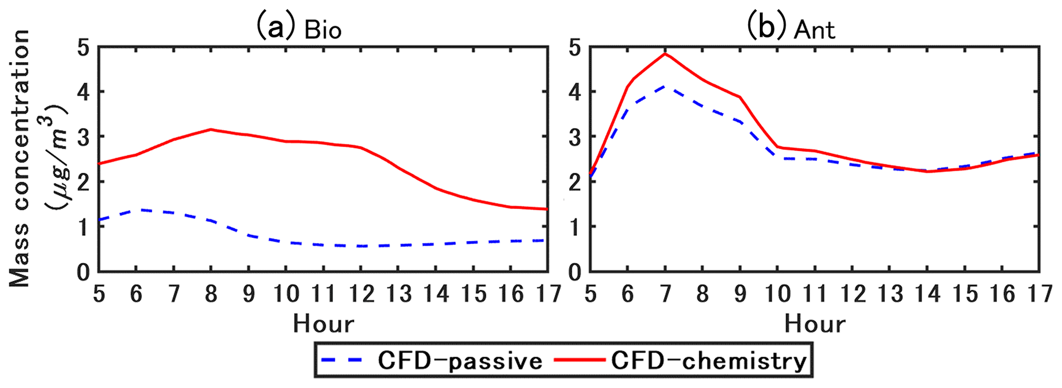
Figure 15Simulated time-varying concentration of organic matter. Bio refers to organic matter formed from biogenic precursors. Ant refers to organic matter formed from anthropogenic precursors.
In CFD–chemistry, Bio concentration is larger than that in CFD–passive. As biogenic precursors are not emitted in the street, the condensation of Bio is due to background precursor gases. As discussed previously, the concentration of ammonium nitrate is higher in CFD–chemistry than in CFD–passive, providing a larger aqueous mass onto which hydrophilic compounds of the biogenic precursor gases condense. As the condensation of ammonium nitrate decreases in the afternoon as shown in Fig. 14, the condensation of Bio also decreases.
Ant is largely influenced by traffic emissions in the street, particularly by emissions of semi-volatile compounds (Sartelet et al., 2018) which soon condense after emissions. Therefore, there is a peak around 07:00 LT owing to the morning rush. In the model, anthropogenic emissions are mostly hydrophobic, therefore the condensation is not enhanced by the increase in inorganic concentrations. Consequently, the difference between CFD–chemistry and CFD–passive is larger in the morning owing to the large increase in traffic emissions, but small differences are observed in the afternoon.
Figure 16 shows the time-averaged concentrations of PM10, PM1, and the chemical compounds of PM10 from 05:00 LT to 17:00 LT. The time-averaged PM10 and PM1 concentrations increase by approximately 3.8 µg m−3 in CFD–chemistry compared to CFD–passive, indicating that chemistry mainly influences small particles. Inert matter slightly decreases in CFD–chemistry owing to dry deposition. Condensation increases by 48 %, 38 %, and 53 % of nitrate, ammonium, and organic matter concentrations, respectively, in CFD–chemistry compared to CFD–passive.
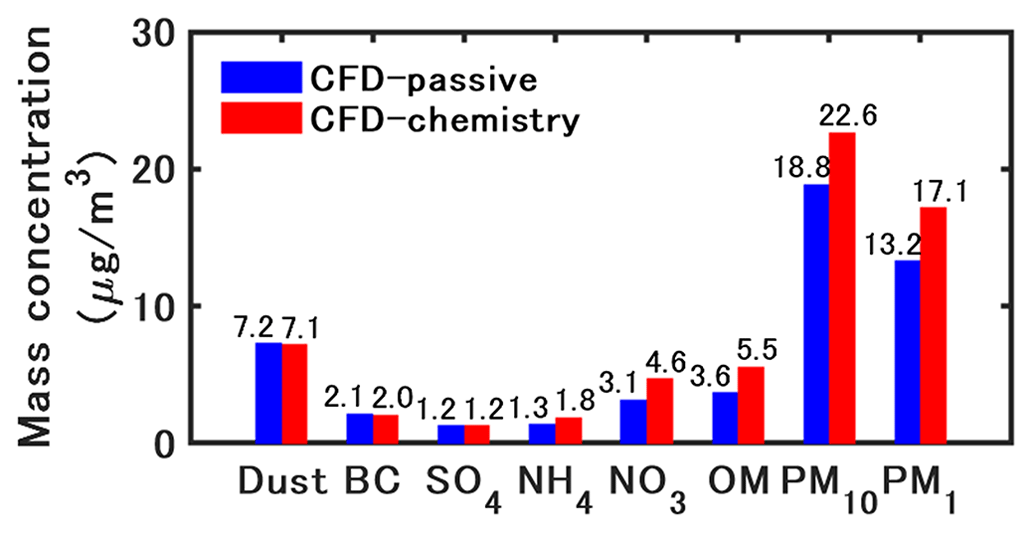
Figure 16Time-averaged concentration of PM10, PM1 and the chemical compounds of PM10 from 05:00 to 17:00.
5.3 Size distribution of particulate matter
Figure 17 shows the time-averaged size distribution of PM10 for the different chemical compounds of particles from 05:00 LT to 17:00 LT. The bound diameters are 0.01, 0.04, 0.16, 0.4, 1.0, 2.5, and 10 µm, and the mean diameters are 0.02, 0.08, 0.25, 0.63, 1.58, and 5.01 µm.

Figure 17Time-averaged size distribution of PM10 for different chemical species from 05:00 LT to 17:00 LT.
For the total concentration of PM10 (Fig. 17a), the lowest and the largest concentrations are in the first size section (0.01–0.04 µm) and the second size section (0.04–0.16 µm) respectively, for both the CFD–passive and the CFD–chemistry simulations. Generally, the loss and gain of mass concentration in each size section are related to emission, dry deposition, coagulation (small particles coagulate into large particles), and condensation/evaporation (phase exchange between gas and particles).
Figure 17b shows the mass concentration ratio between CFD–passive and CFD–chemistry for each size section. For particles in the size range of 0.04–0.16 µm, the concentrations are smaller in CFD–chemistry than in CFD–passive, because dry deposition and coagulation both decrease mass concentration for those particles. Furthermore, semi-volatile gases may evaporate from small particles because of the Kelvin effect and condense onto larger particles. For particles in the size range of 0.16–1.0 µm, the concentrations are much larger in CFD–chemistry than CFD–passive, indicating that coagulation and condensation on the mass-concentration increase are dominant to other processes, such as deposition. For particles larger than 1 µm, the concentrations of CFD–passive and CFD–chemistry are similar because particle dynamics have a low influence on large particles.
The size distribution of dust (Fig. 17c) shows that most dust mass concentrations are in particles larger than 1 µm. Meanwhile, most of the mass concentration of BC, inorganic, and organic matter (Fig. 17d–f) is in particles smaller than 1 µm. Coagulation is the main process influencing the size distribution for inert matter (dust and BC). Compared to CFD–passive, the mass concentration of dust and BC in the second size section decrease by 0.48 and 0.43 µg m−3 in CFD–chemistry. Correspondingly, the mass concentrations of dust and BC in the third size section increase by 0.41 and 0.35 µg m−3.
For inorganic matter, in the second size section, the concentrations are similar in CFD–passive and CFD–chemistry: particle dynamics decrease sulfate concentration by 0.32 µg m−3 and increase nitrate concentration by 0.17 µg m−3. However, because of the results of the combination effect of coagulation and ammonium nitrate condensation, the concentrations largely increase in the third size section in CFD–chemistry: sulfate, ammonium ,and nitrate increase by 0.27, 0.6 and 1.24 µg m−3, respectively.
For organic matter, because of the condensation of hydrophilic compounds from background biogenic gases and anthropogenic emissions, CFD–chemistry leads to a small increase in concentrations (0.53 µg m−3) in the second size section and a large increase in the third section (1.21 µg m−3) compared to CFD–passive. In detail, Bio concentrations increase by 0.89 µg m−3 and Ant concentrations decrease by 0.36 µg m−3 in the second size section. In the third size section, Bio and Ant concentrations increase by 0.67, 0.54 µg m−3.
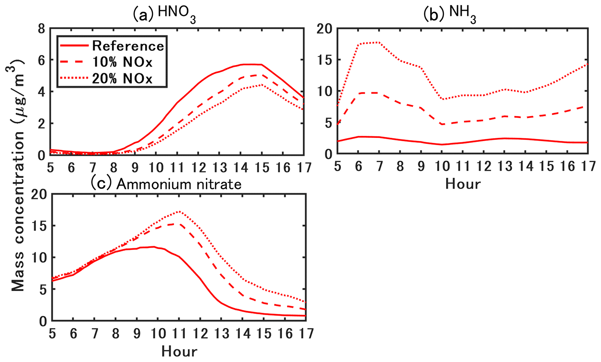
5.4 Influence of ammonia traffic emissions
Suarez-Bertoa et al. (2017) conducted on-road measurements of NH3 emissions from two Euro 6b compliant light-duty cars (one gasoline and one diesel) under real-world driving conditions, and they found that NH3 emissions accounted for 11.9 % and 0.92 % of NOx emissions for gasoline and diesel vehicles. As explained in Sect. 5.2, NH3 emissions are approximately 1 %–2 % of NOx emissions in the reference case. Two cases are considered to simulate the impact of an increase in the fraction of gasoline cars, and sensitivity simulations are performed with NH3 emissions considered as 10 % and 20 % of the NOx emissions.
Figure 18 shows the sensitivity of ammonium nitrate concentration to NH3 emissions. A larger NH3 emission delays the peak of ammonium nitrate by approximately 1 h. For a 12 h average, considering NH3 emissions of 10 % and 20 % of NOx emissions leads to a large increase in ammonium nitrate (35 % and 55 %) compared to the reference case because of the formation of ammonium nitrate by the condensation of HNO3 and NH3.
Particles in urban environment impose adverse impacts on pedestrians' health. Conventional CFD methods regarding particles as passive scalars cannot reproduce the formation of secondary aerosols and may lead to uncertain simulations. Therefore, to increase the simulation accuracy of particle dispersion, we coupled the CFD software OpenFOAM (OF) and Code_Saturne (CS) with SSH-aerosol, a modular box model to simulate the evolution of primary and secondary aerosols. The main processes involved in the aerosol dynamics (coagulation, condensation/evaporation, and dry deposition) were considered.
We simulated a 12 h transient dispersion of pollutants from traffic emissions in a street canyon using the unsteady RANS model. The simulation domain was generated to model a street canyon where field measurements are available. The flow field was based on the WRF model. The background concentrations of gas and particles were obtained from regional-scale simulations with a chemistry transport model. The particle diameter range (0.01 to 10 µm) was divided into six size sections. The following conclusions were drawn from the results of this study.
-
The simulated spatially averaged values in the street canyon were validated from field measurement using validation metrics. For both OF and CS, the simulated NO2 and PM10 concentrations based on the coupling model (CFD–chemistry) achieved better agreement with the measurement data than the conventional CFD simulation which considered pollutants as passive scalars (CFD–passive). The differences between the OF and CS results were not obvious and were mainly due to the differences in the turbulence scheme. The following conclusions were drawn based on the simulated OF concentrations.
-
For the flow field, a large vortex was observed in the canyon with a small secondary vortex at the corner of the leeward wall at the current aspect ratio (). In CFD–chemistry, because of the reverse flow, the 12 h (from 05:00 LT to 17:00 LT) time-averaged NO2 mass concentration, PM10 mass and number concentrations at pedestrian height were much higher near the leeward wall (116, 28, 3.2×10¹⁰ m−3) than the background (26, 15, 2.3×10¹⁰ m−3).
-
Secondary aerosol formation largely affected the mass concentration and size distribution of particulate matter. For 12 h time-averaged concentrations, ammonium nitrate and organic matter increased by 46 % and 53 % in CFD–chemistry compared to CFD–passive because of condensation of HNO3 and NH3, background biogenic precursor gases and anthropogenic precursor gas emissions. Coagulation largely influenced the size distribution of small particles by combining particles with a diameter of 0.04–0.16 µm into 0.16–0.4 µm. At the same time, CFD–chemistry showed a much larger concentration than CFD–passive for the particles in 0.16–1.0 µm, indicating that the effect of condensation on increasing mass concentration was dominant compared to other chemical processes.
-
Urban areas are NH3-limited (HNO3 sufficient) areas, therefore, increasing NH3 leads to a large increase in ammonium nitrate. Vehicles are considered to be the main source of NH3 in urban environments. Increasing the fleet's proportion of recent gasoline vehicles may increase NH3 emissions. For a 12 h average, we considered NH3 emissions of 10 % and 20 % of NOx emissions led to a large increase in ammonium nitrate (35 % and 55 %) compared to the reference case which considers NH3 emissions as 1 %–2 % of NOx emissions.
-
A grid sensitivity analysis showed that the particles' concentrations of inorganic and organic compounds were sensitive to grid resolution, whereas inert particle concentrations were not sensitive to grid resolution. In addition, simulated values based on a grid size of 0.5 m in the street canyon showed small differences with a grid size of 0.25 m, indicating that a spatial resolution of 0.5 m can be enough for reactive particle dispersion at the street level.
-
Operator splitting is often employed to solve the transport term and chemical reactions over a given time step in chemical transport simulations. Two integration orders were considered: A–B splitting method (CFD(Δt)–Chemistry(Δt)) and A–B–A splitting method (CFD()–Chemistry(Δt)–CFD()). The results showed that the A–B–A splitting method had almost the same concentrations as the A–B splitting method with half the computational time. Further sensitivity analysis on the time step showed that a time step of 0.5 s was enough when using the A–B–A splitting method.
-
Conducting a CFD simulation with constant boundary conditions and emission rates at a specific time point is considered a practical method to achieve time-averaged concentrations for evaluating street-level pollutant concentrations. The validation was conducted using conditions on five time points (07:00 LT, 10:00 LT, 13:00 LT, 15:00 LT, and 17:00 LT). The simulated concentration based on the above method exhibited almost the same value as the simulation with transient conditions at the same time points.
The limitation of this study should be addressed as several reasonable approximations and assumptions were made in the simulation settings.
-
Concerning the simulation domain, since we focused on the coupling of gas chemical reactions and particle dynamics to the CFD codes, we selected a 12 h period when wind direction was perpendicular to the street. In that case, a 2-D simplification of the simulation domain is reasonable, as shown by Maison et al. (2022). In addition, the 2-D simplification is frequently adopted for studying dispersion of reactive pollutants in a street canyon (Garmory et al., 2009; Wu et al., 2021). However, in more general cases, the pollutant residence time for a 3-D canyon could be shorter compared to the 2-D canyon adopted in this study, and the effects of chemical reaction or aerosol processes could be weaker than this study reported. In addition, various wind directions should be considered to better evaluate the performance of the coupled model. Further work will focus on the application of the coupled model to a complex urban environment with changing wind directions.
-
Concerning the physical model, the simulations were based on RANS closure, and the SSH-aerosol processed the ensemble-averaged concentration, therefore the covariance of turbulent diffusion and chemical reaction may not be fully reproduced. The simulation based on LES may provide better prediction of second-order quantities. In addition, the radiation on the wall may lead to street-level variations of temperature and could affect the flow field and chemical reaction rates. However, this was not considered here, and the radiation effect on the local temperature was simplified as being the same as in the inflow condition. The inflow temperature was obtained from the WRF model where the radiation was considered, and the time variation of temperature was considered to be the same as the background.
Future work will be conducted on the influence of environmental factors and emission conditions, aiming to provide knowledge to devise suitable countermeasures to decrease particle concentration in microscale urban environments.
The schemes for particle deposition velocity vd were added to the transport equations using volume sink terms based on Zhang et al. (2001) and can be represented as follows:
The deposition velocity for the particles vd,p consists of both gravitational settling and surface deposition near the wall surfaces. The gravitational settling velocity vg was considered for the entire field, ρ is the particle density; dp is the particle diameter; g is the acceleration of gravity; C is Cunningham correction factor for small particles; η is the viscosity coefficient of air.
The aerodynamic resistance Ra is calculated from the first-layer height zR, roughness length z0, Von Kármán constant κ, friction velocity u∗, and stability function ψH. For the k–ε model, u∗ is estimated by and Cμ=0.09 is a constant of the model.
The surface resistance Rs is calculated from u∗, the collection efficiency from Brownian diffusion EB, the impaction EIM and the interception EIN. The correction factor represents the fraction of particles that stick to the surface R1 and an empirical constant ε0=3.
The dry deposition schemes for gas were added to the transport equations using volume sink terms based on Wesely (1989) and Zhang et al. (2003),which can be represented as follows:
The deposition velocity for gas vd,g is calculated from the aerodynamic resistance Ra, the quasi-laminar layer resistance Rb and the surface resistance for gas Rc; and Pr=0.72 are the Schmidt and Prandtl number; υ is the kinematic viscosity of air, and D is the molecular diffusivity of different gases. Rc is calculated based on Zhang et al. (2003).
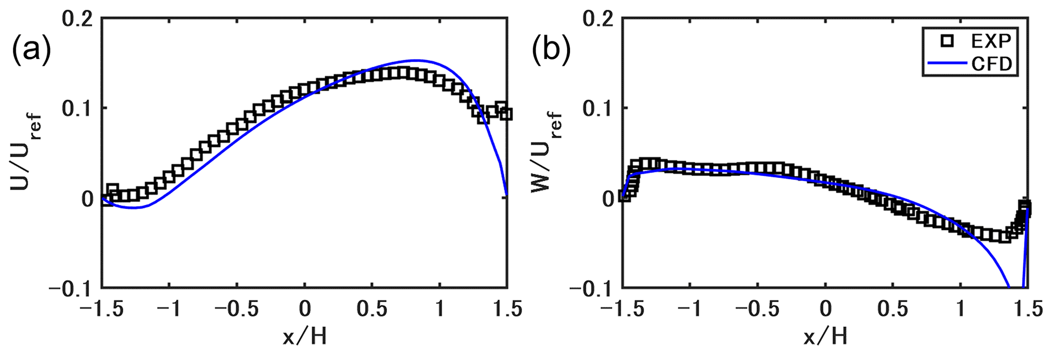
Correctly representing the flow field in the street canyon is important to accurately model the concentrations. Unfortunately, observation data on wind velocity in the street are not available. Therefore, we conducted a velocity validation for OpenFOAM v2012 using data from a wind tunnel experiment (Blackman et al., 2015). The 2-D simulation domain is shown in Fig. B1. The aspect ratio in the experiment () is close to this study (). The building height H is 0.06 m. The grid size is H in x and z directions in the simulation domain under 3H. The free-stream velocity Uref is 5.9 m s−1. The steady-state flow field is simulated with the same turbulence model (RNG k–ε model) as in the paper, and cyclic boundary conditions are used for the inlet and outlet. The slip boundary is considered for the top, and non-slip boundary conditions with the same wall functions as in the paper are considered for other walls.
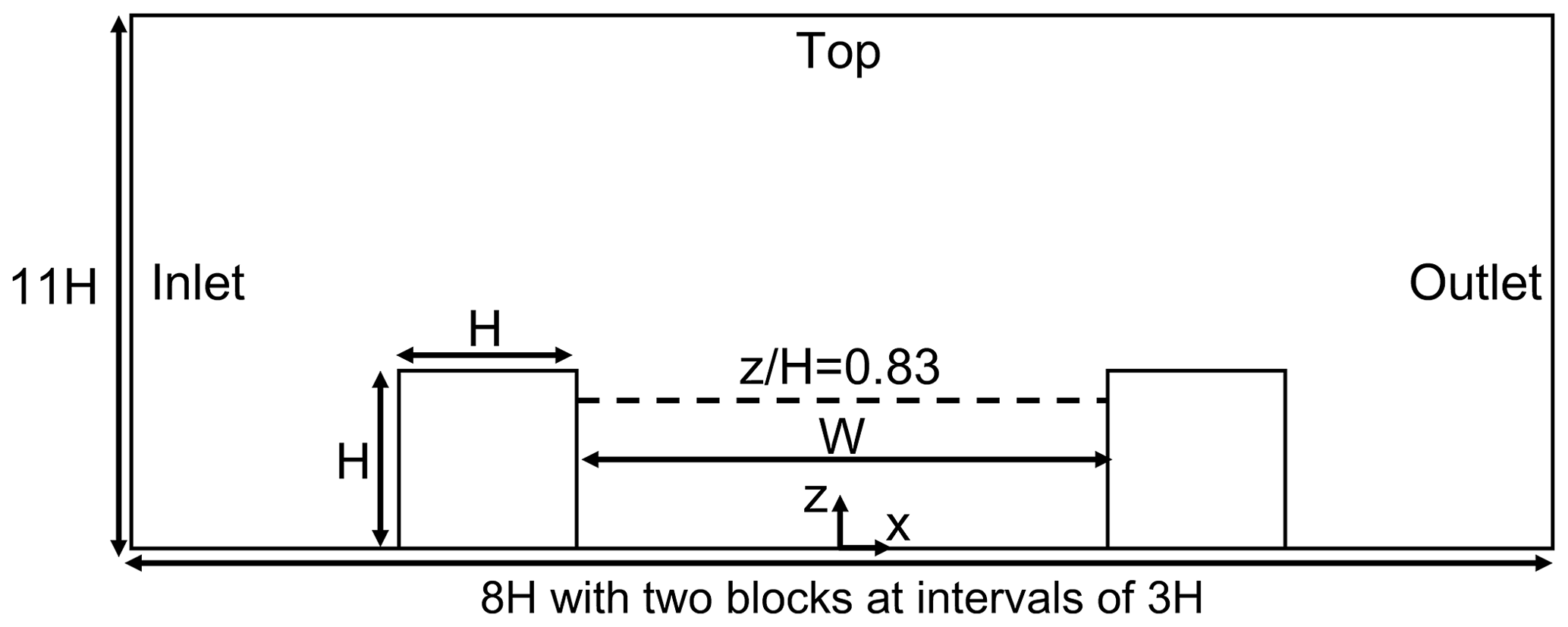
Figure B2 compares the simulated streamwise and vertical direction of mean wind velocities with the experimental values at . The RNG k–ε model reproduces the velocities well, although the velocities very close to the windward wall show differences with the experimental values. The above validation shows that if suitable inlet conditions are given, the flow field is well reproduced with the turbulence model adopted in this study.
The codes and datasets in this publication are available to the community, and they can be accessed by request to the corresponding author.
KS and RO were responsible for conceptualization. CL, YW, CF, KS, YK, and ZW developed the software. CL and YW conducted the visualization and validation; CL, YW, and KS performed the formal analysis. KS and RO acquired resources. CL, YW, RO, and KS were responsible for writing and original draft preparation. CF, YK, and HK reviewed and edited the paper. All co-authors contributed to the discussion of the paper.
The contact author has declared that none of the authors has any competing interests.
Publisher’s note: Copernicus Publications remains neutral with regard to jurisdictional claims in published maps and institutional affiliations.
This article is part of the special issue “Air quality research at street level (ACP/GMD inter-journal SI)”. It is not associated with a conference.
This work benefited from discussions with Bertrand Carissimo.
This research has been supported by DIM QI2 (Air Quality Research Network on air quality in the Île-de-France region) and by the Île-de-France region.
This paper was edited by Yang Zhang and reviewed by three anonymous referees.
Anenberg, S. C., Miller, J., Minjares, R., Du, L., Henze, D. K., Lacey, F., Malley, C. S., Emberson, L., Franco, V., Klimont, Z., and Heyes, C.: Impacts and mitigation of excess diesel-related NO x emissions in 11 major vehicle markets, Nature, 545, 467–471, https://doi.org/10.1038/nature22086, 2017.
Archambeau, F., Méchitoua, N., and Sakiz, M.: Code Saturne: A Finite Volume Code for Turbulent flows – Industrial Applications, International Journal on Finite Volumes, 1, https://hal.science/hal-01115371, 2004.
Arpaci, V. S. and Larsen, P. S.: Convection Heat Transfer, Prentice Hall, New York, ISBN 10. 0131723464, ISBN-13. 978-0131723467, 1984.
Belcher, S. E.: Mixing and transport in urban areas, Philosophical Transactions of the Royal Society A: Mathematical, Phys. Eng. Sci., 363, 2947–2968, https://doi.org/10.1098/rsta.2005.1673, 2005.
Bishop, G. A. and Stedman, D. H.: Reactive Nitrogen Species Emission Trends in Three Light-/Medium-Duty United States Fleets, Environ Sci Technol, 49, 11234–11240, https://doi.org/10.1021/acs.est.5b02392, 2015.
Blackman, K., Perret, L., and Savory, E.: Effect of upstream flow regime on street canyon flow mean turbulence statistics, Environ. Fluid Mech., 15, 823–849, https://doi.org/10.1007/s10652-014-9386-8, 2015.
Blocken, B., Tominaga, Y., and Stathopoulos, T.: CFD simulation of micro-scale pollutant dispersion in the built environment, Build Environ., 64, 225–230, https://doi.org/10.1016/j.buildenv.2013.01.001, 2013.
Chang, J. C. and Hanna, S. R.: Air quality model performance evaluation, Meteorol. Atmos. Phys., 87, 167–196, https://doi.org/10.1007/s00703-003-0070-7, 2004.
Di Sabatino, S., Buccolieri, R., Pulvirenti, B., and Britter, R.: Simulations of pollutant dispersion within idealised urban-type geometries with CFD and integral models, Atmos. Environ., 41, 8316–8329, https://doi.org/10.1016/j.atmosenv.2007.06.052, 2007.
Du, Y., Xu, X., Chu, M., Guo, Y., and Wang, J.: Air particulate matter and cardiovascular disease: The epidemiological, biomedical and clinical evidence, J. Thorac. Dis., 8, E8–E19, https://doi.org/10.3978/j.issn.2072-1439.2015.11.37, 2016.
EMEP/EEA: EMEP/EEA air pollutant emission inventory guidebook 2019, EEA Report No 13/2019, European Environment Agency: https://www.eea.europa.eu/publications/emep-eea-guidebook-2019 (last access: 14 March 2022), 2019.
Ferrero, E., Alessandrini, S., Anderson, B., Tomasi, E., Jimenez, P., and Meech, S.: Lagrangian simulation of smoke plume from fire and validation using ground-based lidar and aircraft measurements, Atmos. Environ., 213, 659–674, https://doi.org/10.1016/j.atmosenv.2019.06.049, 2019.
Fu, K. and Liang, D.: The conservative characteristic FD methods for atmospheric aerosol transport problems, J. Comput. Phys., 305, 494–520, https://doi.org/10.1016/j.jcp.2015.10.049, 2016.
Gao, S., Kurppa, M., Chan, C. K., and Ngan, K.: Technical note: Dispersion of cooking-generated aerosols from an urban street canyon, Atmos. Chem. Phys., 22, 2703–2726, https://doi.org/10.5194/acp-22-2703-2022, 2022.
Guimet, V. and Laurence, D.: A linearised turbulent production in the k-ε model for engineering applications, in: Engineering Turbulence Modelling and Experiments 5, edited by: Rodi, W. and Fueyo, N., Elsevier Science Ltd, Oxford, UK, 157–166, https://doi.org/10.1016/B978-008044114-6/50014-4, 2002.
Hanna, S. R., Hansen, O. R., and Dharmavaram, S.: FLACS CFD air quality model performance evaluation with Kit Fox, MUST, Prairie Grass, and EMU observations, Atmos. Environ., 38, 4675–4687, https://doi.org/10.1016/j.atmosenv.2004.05.041, 2004.
Harten, A.: On a Class of High Resolution Total-Variation-Stable Finite-Difference Schemes, SIAM J. Numer. Anal., 21, 1–23, https://doi.org/10.1137/0721001, 1984.
Jones, A. M., Yin, J., and Harrison, R. M.: The weekday–weekend difference and the estimation of the non-vehicle contributions to the urban increment of airborne particulate matter, Atmos. Environ., 42, 4467–4479, https://doi.org/10.1016/j.atmosenv.2008.02.001, 2008.
Kim, M. J.: Sensitivity of nitrate aerosol production to vehicular emissions in an urban street, Atmosphere (Basel), 10, 212, https://doi.org/10.3390/ATMOS10040212, 2019.
Kim, M. J., Park, R. J., Kim, J. J., Park, S. H., Chang, L. S., Lee, D. G., and Choi, J. Y.: Computational fluid dynamics simulation of reactive fine particulate matter in a street canyon, Atmos. Environ., 209, 54–66, https://doi.org/10.1016/j.atmosenv.2019.04.013, 2019.
Kim, Y., Wu, Y., Seigneur, C., and Roustan, Y.: Multi-scale modeling of urban air pollution: development and application of a Street-in-Grid model (v1.0) by coupling MUNICH (v1.0) and Polair3D (v1.8.1), Geosci. Model Dev., 11, 611–629, https://doi.org/10.5194/gmd-11-611-2018, 2018.
Kim, Y., Lugon, L., Maison, A., Sarica, T., Roustan, Y., Valari, M., Zhang, Y., André, M., and Sartelet, K.: MUNICH v2.0: a street-network model coupled with SSH-aerosol (v1.2) for multi-pollutant modelling, Geosci. Model Dev., 15, 7371–7396, https://doi.org/10.5194/gmd-15-7371-2022, 2022.
Kumar, P., Fennell, P., Langley, D., and Britter, R.: Pseudo-simultaneous measurements for the vertical variation of coarse, fine and ultrafine particles in an urban street canyon, Atmos. Environ., 42, 4304–4319, https://doi.org/10.1016/j.atmosenv.2008.01.010, 2008.
Kurppa, M., Hellsten, A., Roldin, P., Kokkola, H., Tonttila, J., Auvinen, M., Kent, C., Kumar, P., Maronga, B., and Järvi, L.: Implementation of the sectional aerosol module SALSA2.0 into the PALM model system 6.0: model development and first evaluation, Geosci. Model Dev., 12, 1403–1422, https://doi.org/10.5194/gmd-12-1403-2019, 2019.
Lo, K. W. and Ngan, K.: Characterising the pollutant ventilation characteristics of street canyons using the tracer age and age spectrum, Atmos. Environ., 122, 611–621, https://doi.org/10.1016/j.atmosenv.2015.10.023, 2015.
Lo, K. W. and Ngan, K.: Characterizing ventilation and exposure in street canyons using Lagrangian particles, J. Appl. Meteorol. Climatol., 56, 1177–1194, https://doi.org/10.1175/JAMC-D-16-0168.1, 2017.
Lugon, L., Vigneron, J., Debert, C., Chrétien, O., and Sartelet, K.: Black carbon modeling in urban areas: investigating the influence of resuspension and non-exhaust emissions in streets using the Street-in-Grid model for inert particles (SinG-inert), Geosci. Model Dev., 14, 7001–7019, https://doi.org/10.5194/gmd-14-7001-2021, 2021a.
Lugon, L., Sartelet, K., Kim, Y., Vigneron, J., and Chretien, O.: Simulation of primary and secondary particles in the streets of Paris using MUNICH, Faraday Discuss., 226, 432–456, https://doi.org/10.1039/d0fd00092b, 2021b.
Maison, A., Flageul, C., Carissimo, B., Wang, Y., Tuzet, A., and Sartelet, K.: Parameterizing the aerodynamic effect of trees in street canyons for the street network model MUNICH using the CFD model Code_Saturne, Atmos. Chem. Phys., 22, 9369–9388, https://doi.org/10.5194/acp-22-9369-2022, 2022.
Mallet, V., Quélo, D., Sportisse, B., Ahmed de Biasi, M., Debry, É., Korsakissok, I., Wu, L., Roustan, Y., Sartelet, K., Tombette, M., and Foudhil, H.: Technical Note: The air quality modeling system Polyphemus, Atmos. Chem. Phys., 7, 5479–5487, https://doi.org/10.5194/acp-7-5479-2007, 2007.
OpenFOAM user guide: https://www.openfoam.com/, 1 December 2022.
Parente, A., Gorlé, C., van Beeck, J., and Benocci, C.: Improved k–ε model and wall function formulation for the RANS simulation of ABL flows, J. Wind Eng. Ind. Aerod., 99, 267–278, https://doi.org/10.1016/j.jweia.2010.12.017, 2011.
Sartelet, K., Zhu, S., Moukhtar, S., André, M., André, J. M., Gros, V., Favez, O., Brasseur, A., and Redaelli, M.: Emission of intermediate, semi and low volatile organic compounds from traffic and their impact on secondary organic aerosol concentrations over Greater Paris, Atmos. Environ., 180, 126–137, https://doi.org/10.1016/j.atmosenv.2018.02.031, 2018.
Sartelet, K., Couvidat, F., Wang, Z., Flageul, C., and Kim, Y.: SSH-aerosol v1.1: A modular box model to simulate the evolution of primary and secondary aerosols, Atmosphere (Basel), 11, 525, https://doi.org/10.3390/atmos11050525, 2020.
Sartelet, K., Kim, Y., Couvidat, F., Merkel, M., Petäjä, T., Sciare, J., and Wiedensohler, A.: Influence of emission size distribution and nucleation on number concentrations over Greater Paris, Atmos. Chem. Phys., 22, 8579–8596, https://doi.org/10.5194/acp-22-8579-2022, 2022.
Sartelet, K. N., Debry, E., Fahey, K., Roustan, Y., Tombette, M., and Sportisse, B.: Simulation of aerosols and gas-phase species over Europe with the Polyphemus system: Part I-Model-to-data comparison for 2001, Atmos. Environ., 41, 6116–6131, https://doi.org/10.1016/j.atmosenv.2007.04.024, 2007.
Sportisse, B.: An Analysis of Operator Splitting Techniques in the Stiff Case, J. Comput. Phys., 161, 140–168, https://doi.org/10.1006/jcph.2000.6495, 2000.
Stelson, A. W. and Seinfeld, J. H.: Relative humidity and temperature dependence of the ammonium nitrate dissociation constant, Atmos. Environ. (1967), 16, 983–992, https://doi.org/10.1016/0004-6981(82)90184-6, 1982.
Suarez-Bertoa, R. and Astorga, C.: Impact of cold temperature on Euro 6 passenger car emissions, Environ. Pollut., 234, 318–329, https://doi.org/10.1016/j.envpol.2017.10.096, 2018.
Suarez-Bertoa, R., Mendoza-Villafuerte, P., Riccobono, F., Vojtisek, M., Pechout, M., Perujo, A., and Astorga, C.: On-road measurement of NH 3 emissions from gasoline and diesel passenger cars during real world driving conditions, Atmos. Environ., 166, 488–497, https://doi.org/10.1016/j.atmosenv.2017.07.056, 2017.
Sun, K., Tao, L., Miller, D. J., Pan, D., Golston, L. M., Zondlo, M. A., Griffin, R. J., Wallace, H. W., Leong, Y. J., Yang, M. M., Zhang, Y., Mauzerall, D. L., and Zhu, T.: Vehicle Emissions as an Important Urban Ammonia Source in the United States and China, Environ. Sci. Technol., 51, 2472–2481, https://doi.org/10.1021/acs.est.6b02805, 2017.
Sung, J. C., Pulliam, B. L., and Edwards, D. A.: Nanoparticles for drug delivery to the lungs, Trends Biotechnol., 25, 563–570, https://doi.org/10.1016/j.tibtech.2007.09.005, 2007.
Tominaga, Y. and Stathopoulos, T.: Turbulent Schmidt numbers for CFD analysis with various types of flowfield, Atmos. Environ., 41, 8091–8099, https://doi.org/10.1016/j.atmosenv.2007.06.054, 2007.
Tominaga, Y. and Stathopoulos, T.: CFD simulation of near-field pollutant dispersion in the urban environment: A review of current modeling techniques, Atmos. Environ., 79, 716–730, https://doi.org/10.1016/j.atmosenv.2013.07.028, 2013.
Trini Castelli, S., Armand, P., Tinarelli, G., Duchenne, C., and Nibart, M.: Validation of a Lagrangian particle dispersion model with wind tunnel and field experiments in urban environment, Atmos. Environ., 193, 273–289, https://doi.org/10.1016/j.atmosenv.2018.08.045, 2018.
Wesely, M. L.: Parameterization of surface resistances to gaseous dry deposition in regional-scale numerical models, Atmos. Environ. (1967), 23, 1293–1304, https://doi.org/10.1016/0004-6981(89)90153-4, 1989.
Wu, L., Hang, J., Wang, X., Shao, M., and Gong, C.: APFoam 1.0: integrated computational fluid dynamics simulation of O3–NOx–volatile organic compound chemistry and pollutant dispersion in a typical street canyon, Geosci. Model Dev., 14, 4655–4681, https://doi.org/10.5194/gmd-14-4655-2021, 2021.
Yakhot, V., Orszag, S. A., Thangam, S., Gatski, T. B., and Speziale, C. G.: Development of turbulence models for shear flows by a double expansion technique, Phys. Fluids A, 4, 1510–1520, https://doi.org/10.1063/1.858424, 1992.
Yee, H. C.: Construction of explicit and implicit symmetric TVD schemes and their applications, J. Comput. Phys., 68, 151–179, https://doi.org/10.1016/0021-9991(87)90049-0, 1987.
Zhang, K., Chen, G., Zhang, Y., Liu, S., Wang, X., Wang, B., and Hang, J.: Integrated impacts of turbulent mixing and NOX-O3 photochemistry on reactive pollutant dispersion and intake fraction in shallow and deep street canyons, Sci. Total Environ., 712, 135553, https://doi.org/10.1016/j.scitotenv.2019.135553, 2020.
Zhang, L., Gong, S., Padro, J., and Barrie, L.: A size-segregated particle dry deposition scheme for an atmospheric aerosol module, Atmos. Environ., 35, 549–560, https://doi.org/10.1016/S1352-2310(00)00326-5, 2001.
Zhang, L., Brook, J. R., and Vet, R.: A revised parameterization for gaseous dry deposition in air-quality models, Atmos. Chem. Phys., 3, 2067–2082, https://doi.org/10.5194/acp-3-2067-2003, 2003.