Sensitivity of cirrus and contrail radiative effect on cloud microphysical and environmental parameters

Natural cirrus clouds and contrails cover about 30 % of the Earth's mid-latitudes and up to 70 % of the tropics. Due to their widespread occurrence, cirrus clouds have a considerable impact on the Earth energy budget, which, on average, leads to a warming net radiative effect (solar + thermal infrared). However, whether the instantaneous radiative effect (RE), which in some cases corresponds to a radiative forcing, of natural cirrus or contrails is positive or negative depends on their microphysical, macrophysical, and optical properties, as well as the radiative properties of the environment. This is further complicated by the fact that the actual ice crystal shape is often unknown, and thus, ice clouds remain one of the components that are least understood in the Earth's radiative budget.

The present study aims to investigate the dependency of the effect on cirrus RE on eight parameters, namely solar zenith angle, ice water content, ice crystal effective radius, cirrus temperature, surface albedo, surface temperature, cloud optical thickness of an underlying liquid water cloud, and three ice crystal shapes. In total, 283 500 plane-parallel radiative transfer simulations have been performed, not including three-dimensional scattering effects. Parameter ranges are selected that are typically associated with natural cirrus and contrails. In addition, the effect of variations in the relative humidity profile and the ice cloud geometric thickness have been investigated for a sub-set of the simulations. The multi-dimensionality and complexity of the eight-dimensional parameter space makes it impractical to discuss all potential configurations in detail. Therefore, specific cases are selected and discussed.

For a given parameter combination, the largest impact on solar, thermal-infrared (TIR), and net RE is related to the ice crystal effective radius. The second most important parameter is ice water content, which equally impacts the solar and terrestrial RE. The solar RE of cirrus is also determined by solar zenith angle, surface albedo, liquid cloud optical thickness, and ice crystal shape (in descending priority). RE in the TIR spectrum is dominated by surface temperature, ice cloud temperature, liquid water cloud optical thickness, and ice crystal shape. Net RE is controlled by surface albedo, solar zenith angle, and surface temperature in decreasing importance. The relative importance of the studied parameters differs, depending on the ambient conditions. Furthermore, and during nighttime the net RE is equal to the TIR RE.

The data set generated in this work is publicly available. It can be used as a lookup table to extract the RE of cirrus clouds, contrails, and contrail cirrus instead of full radiative transfer calculations.

1 Introduction

Cirrus clouds cover large areas of the Earth, with cloud cover estimates of 30 % in the mid-latitudes and up to 70 % in the tropics (Liou, 1986; Wylie and Menzel, 1999; Chen et al., 2000; Sassen et al., 2008; Nazaryan et al., 2008). Due to their widespread occurrence, cirrus can have a considerable impact on the global energy budget. In addition to cirrus, air traffic leads to the formation of condensation trails, also termed contrails, which are geometrically and optically thin clouds with similar radiative effects as thin natural cirrus (Liou, 1986). For the sake of simplicity, the term cirrus is used interchangeably for natural cirrus, contrail-induced cirrus, and contrails throughout this article.

Depending on ambient conditions, contrails are short-lived (t<10 min) but can persist up to a day, when the surrounding air mass is sufficiently cold and moist (Schumann, 1996; Haywood et al., 2009; Schumann and Heymsfield, 2017; Kärcher, 2018). In such conditions, persistent contrails transition from line-shaped clouds to larger cloud fields (Unterstrasser and Stephan, 2020). Modeling and satellite studies have estimated that contrail and contrail-induced cirrus cloud cover can reach up to 6 % to 10 % over Europe (Burkhardt and Kärcher, 2011; Quaas et al., 2021) and significantly contribute to high-level cloudiness over Europe (Schumann et al., 2015, 2021).

Under most circumstances, cirrus clouds have a cooling effect in the solar wavelength range (0.2–3.5 µm; sometimes called shortwave) and a heating effect in the thermal-infrared (TIR) wavelength range (3.5–75 µm; sometimes also termed longwave or terrestrial). The net radiative effect (solar cooling + TIR warming) is often a warming, as the TIR effect dominates (Chen et al., 2000). By combining satellite observations and radiative transfer (RT) simulations, Chen et al. (2000) estimated a global annual mean cirrus cloud radiative effect (RE) of −25.3 W m⁻² in the solar wavelength range and 30.7 W m⁻² in the TIR wavelength range, leading to a positive net effect of 5.4 W m⁻². However, whether the instantaneous RE of natural cirrus or contrails is positive or negative depends on their microphysical, macrophysical, and optical, as well as radiative, properties of the environment. The cloud properties relevant to the RE of the cloud are primarily cloud altitude, cloud temperature, ice water content, ice crystal shape (also called crystal habit), and the orientation of the ice crystals (Fu and Liou, 1993; Stephens et al., 2004; Campbell et al., 2016). Furthermore, the underlying surface properties, i.e., surface albedo and surface temperature, and gaseous absorption and additional underlying cloud layers also have an effect on the cirrus RE. Dynamical processes in the atmosphere have a strong influence on those parameters, for example, lifting of air masses along warm conveyor belts or cloud anvils that lead to a variety of ice crystal shapes and crystal surface roughness (Freudenthaler et al., 1996; Wendisch et al., 2007; Yang et al., 2010; Krämer et al., 2016; Luebke et al., 2016). As a result, the actual distribution of crystal shapes within a cirrus and the related RE is often unclear. Thus, ice clouds remain one of the components that are least understood in the Earth's radiative budget (Stevens and Bony, 2013; Bauer et al., 2015; Bickel et al., 2020), and this lack of understanding contributes to uncertainties in the climate impact of aviation (Lee et al., 2021).

To estimate the radiative impact of a cloud and related potential uncertainties and sensitivities, RT simulations represent a helpful tool. While the atmospheric RT in liquid water clouds composed of spherical cloud droplets can rely on geometric optics or Mie scattering theory (Mie, 1908; van de Hulst, 1981), RT in ice clouds is complicated by the non-spherical crystal shape and the interaction with incoming radiation, i.e., through their single-scattering phase function. The single-scattering phase function, for example, has to be determined by computationally expensive methods, like ray tracing (Bi et al., 2014), Monte Carlo simulations (Macke et al., 1996a, b), or the transition matrix (T matrix) method (Mishchenko, 2020). Due to the computational burden of such accurate simulations, parameterizations of ice crystal properties are often developed and validated against the more precise calculations (Takano and Liou, 1989; Fu, 1996; Yang et al., 2000, 2013). More recent ice crystal parameterizations by Yang et al. (2000), Baum et al. (2005a, b), Baum et al. (2007), and Yang et al. (2013) in combination with the latest RT models allow us to determine the radiative impact of cirrus clouds with an acceptable computational cost and accuracy. By varying the microphysical and macrophysical properties of the cirrus, as well as the surface properties in the RT model, the natural range of cirrus and their environment can be represented, and the RE can be estimated. Furthermore, uncertainties due to the insufficiently known crystal shape can be assessed.

Multiple studies that aimed to investigate the impact of a certain parameter on cloud RE have been performed in the past. Fu and Liou (1993) and Yang et al. (2010) focused on the effects of the selected ice crystal habit and ice water path. The effect of the ice crystal size distribution was analyzed, for example, by Zhang et al. (1999) or Mitchell et al. (2011). A comprehensive study of cirrus radiative effects was conducted by Schumann (2012), who aimed to derive a parameterization to estimate the cloud RE. While those studies are valuable, none of them investigates the effect of multiple factors like relevant cloud and environmental input parameters. These studies have identified parameters that affect cirrus RE, but all of these parameters need to be considered together, including both cloud and environmental parameters. This article is intended as a parametric sensitivity study that aims to compare the effects of major parameters. Furthermore, we identify the driving parameters of RE by sampling the input parameter range, which is restricted to values that are typically associated with ice clouds. Finally, we provide an open-access data set, which allows the user to extract cloud REs for user-specific combinations of the input parameters. The lookup table could in fact be coupled with models of any complexity, as long as they simulate the dimensions of the data set, namely solar zenith angle (SZA), ice cloud temperature, surface albedo, ice water content, surface temperature, ice crystal effective radius, and liquid water cloud optical thickness.

The study is structured in the following way. Section 2 introduces the selected parameter space, the RT model, and outlines basic definitions, as well as methods, used in the paper. Subsequently, Sect. 3 presents the results from the RT simulations. Because our simulations assume plane-parallel atmosphere and homogeneous clouds, Sect. 4 discusses three-dimensional RT. That is followed by the summary in Sect. 5.

2 Methods and definitions

2.1 Definition of radiative effect and albedo

The radiative impact of a perturbation, e.g., clouds, is quantified by the concept of the radiative effect (RE). The RE is defined as the net difference in the downward and upward irradiance ($F^{\downarrow }-F^{\uparrow }$) between the perturbed and unperturbed condition. In the case of clouds, the cloud radiative effect (CRE; denoted here as ΔF) is the difference in the fluxes between the cloud (F_c) and cloud-free (F_cf) atmosphere at a given altitude z (Ramanathan et al., 1989; Stapf et al., 2021; Luebke et al., 2022):

$$\begin{array}{}\text{(1)}& \begin{array}{rl}\mathrm{\Delta }F\left(z\right)& =F_{\mathrm{c}}\left(z\right)-F_{\mathrm{cf}}\left(z\right)\\ & ={\left[F^{\downarrow }\left(z\right)-F^{\uparrow }\left(z\right)\right]}_{\mathrm{c}}-{\left[F^{\downarrow }\left(z\right)-F^{\uparrow }\left(z\right)\right]}_{\mathrm{cf}},\end{array}\end{array}$$

where the upward and downward and cloudy and cloud-free irradiances are all counted to be positive. The net RE is given by

$$\begin{array}{}\text{(2)}& \mathrm{\Delta }{F}_{\mathrm{net}}\left(z\right)=\mathrm{\Delta }{F}_{\mathrm{sol}}\left(z\right)+\mathrm{\Delta }{F}_{\mathrm{TIR}}\left(z\right),\end{array}$$

which can be split into a solar and a thermal-infrared component. Within this study, the CRE is calculated for the top of the atmosphere (TOA), which is set in the radiative transfer calculations to an altitude of 120 km, unless stated otherwise.

In addition to the RE, the albedo α describes the interaction of a cloudy scene or a surface with the solar incident radiation. The scene albedo α_sol(z=TOA) at the TOA is defined as the ratio of the reflected upward irradiance $F_{\mathrm{sol}}^{\uparrow }$ at the TOA in relation to the incident downward irradiance $F_{\mathrm{sol}}^{\downarrow }$ at the TOA and is given by

$$\begin{array}{}\text{(3)}& {\mathit{\alpha }}_{\mathrm{sol},\mathrm{TOA}}={\displaystyle \frac{F_{\mathrm{sol}}^{\uparrow }(z=\mathrm{TOA})}{F_{\mathrm{sol}}^{\downarrow }(z=\mathrm{TOA})}}.\end{array}$$

Similarly, the surface albedo α_sol,srf is calculated with $F_{\mathrm{sol},\mathrm{srf}}^{\uparrow }$ and $F_{\mathrm{sol},\mathrm{srf}}^{\downarrow }$ to find the respective irradiances at the surface (z=0 km).

2.2 Radiative transfer simulation setup

Upward and downward irradiances $F^{\uparrow }/F^{\downarrow }$ were simulated with the library for radiative transfer (libRadtran; Emde et al., 2016). The solar irradiances F_sol cover a wavelength range from 0.3 to 3.5 µm, which represents 97.7 % of the total incoming solar radiation (0–10 µm) calculated from the spectrum provided by Kurucz (1994). The thermal-infrared (TIR) irradiances include wavelengths from 3.5 to 75 µm, representing 99.3 % of the integrated blackbody radiation (3.5 to 100 µm) at 285 K (12 ^∘C).

The RT simulations are performed with the one-dimensional (1D) solver DISORT (Stamnes et al., 1988; Buras et al., 2011), which is part of libRadtran. Clouds are assumed to be horizontally uniform, and lateral photon transport between columns is neglected, which is called the independent pixel approximation (IPA; Stephens et al., 1991; Cahalan et al., 1994). As the main objective of this study is to map the basic dependencies of ΔF on the driving parameters, we neglect any variability in the spatial ice water content (IWC) distribution that exists in cirrus (Minnis et al., 1999). We also restrict the simulations to fully cloud-covered scenes. The required number of streams was iteratively determined and set to 16 streams, which provides sufficient accuracy, while limiting the computational time. The trade-off between accuracy and computational time is detailed in Appendix C. The spectral TOA solar irradiance is provided by Kurucz (1994). The RT simulations consider molecular absorption using the coarse-resolution REPTRAN parameterization from Gasteiger et al. (2014). Appendix C provides an uncertainty estimation related to the REPTRAN resolution. Absorption by water vapor, carbon dioxide, ozone, nitrous oxide, carbon monoxide, methane, oxygen, nitrogen, and nitrogen dioxide is included in the simulations (Anderson et al., 1986; Emde et al., 2016).

Table 1 Surface temperature, cloud-top temperature, cloud-top altitude, and cloud-top pressure level of the liquid water and ice water cloud, depending on the atmosphere profile.

The sensitivity of solar, TIR, and net cloud RE ΔF is estimated by varying eight parameters. The parameter ranges were chosen to represent commonly observed cirrus and contrail cirrus properties, as well as environmental parameters.

• The daily course of the Sun position is represented by solar zenith angles θ ranging from 0 and 85^∘. Larger θ values are omitted to avoid numerical instability that would require more streams in the calculation. Furthermore, RT simulations with the DISORT solver for θ>85^∘ have to be interpreted with caution, as DISORT does not consider the sphericity of the Earth and treats atmospheric layers as plane parallel (Stamnes et al., 1988; Buras et al., 2011). In addition, differences between 1D and three-dimensional (3D) RT simulations increase significantly with values of up to 40 % (Gounou and Hogan, 2007; Forster et al., 2012).

• The Earth's surface albedo, α_srf, ranges from 0 to 1, which represents the full possible range. In general, α_srf varies spectrally but is kept constant here for all solar wavelengths. It is varied between 0 and 1 to include surface conditions ranging from open ocean to full sea ice or snow (Baldridge et al., 2009; Gardner and Sharp, 2010; Meerdink et al., 2019; Gueymard et al., 2019). Values of α_srf are given in Table 4. In the TIR wavelength range, α_srf is assumed to be 0, which leads to an emissivity ϵ=1, with the Earth's surface thus acting as a blackbody (Wilber, 1999).

• Three atmospheric profiles (APs) are selected to represent sub-Arctic, mid-latitude, and tropical conditions. The simulations are based on the sub-Arctic winter (afglsw), the US standard (afglus), and the tropical (afglt) profiles, after Anderson et al. (1986). Surface temperatures T_srf of −15.95 ^∘C (sub-Arctic winter), 14.85 ^∘C (US standard), and 26.55 ^∘C (tropical) are defined in libRadtran by the lowermost temperature in the APs. The profile of relative humidity is linked to the AP via the Clausius–Clapeyron equation (Corti and Peter, 2009). Variations in the water vapor (WV) profile primarily impact the RT in the TIR wavelength range, particularly in WV absorption bands, while RT in the solar wavelength range is less affected (Liou, 1992). The cirrus cloud-top temperatures T_cld,ice are selected to span the temperature range in which contrails and cirrus typically form (Krämer et al., 2020). Here we cover a range from 219 to 243 K. The resulting ice cloud-top altitudes z_ice,CT are set to the altitude, where the temperature in the APs equals the desired T_cld,ice. z_ice,CT is found by linear interpolation between the altitude and temperature levels. Cirrus temperatures and related z_ice,CT are listed in Table 1. Within the simulations, the ice cloud geometric thickness dz is set to 1000 m for all simulations, which represents an average for observed contrails and natural cirrus (Freudenthaler et al., 1995; Sassen and Campbell, 2001; Noël and Haeffelin, 2007; Iwabuchi et al., 2012).

• Three different ice crystal shapes are used, namely: (i) moderately rough aggregates of eight-element columns (called aggregates hereafter), which are agglomerations of eight-columnar ice crystals; (ii) “droxtals”, which are almost spherical ice crystals; and (iii) “plates”. These three shapes are selected to represent different stages in the temporal evolution of contrails. Several airborne in situ measurement campaigns that targeted cirrus and contrails imply that aggregates are the dominating ice crystal habit (Liu et al., 2014; Holz et al., 2016; Järvinen et al., 2018). For example, Järvinen et al. (2018) found that 61 % to 81 % of the sampled ice crystals had complex shapes. They further noted that severely roughened column aggregates resemble their observations best. Such ice crystals are also assumed in current remote sensing applications of ice cloud, e.g., in the redefined ice optical properties used by the Moderate Resolution Imaging Spectroradiometer (MODIS) Collection 6 product (Yang et al., 2013; Holz et al., 2016; Platnick et al., 2017; Forster and Mayer, 2022). Furthermore, Forster and Mayer (2022) found mixtures of severely roughened (60 %) and smoothed (40 %) eight-column aggregates to best match observations of (thin) cirrus. As a compromise, we selected moderately rough eight-column aggregates to be the primary ice crystal habit. The second most observed habit is plate-like ice crystals (Holz et al., 2016; Forster et al., 2017; Järvinen et al., 2018), which are included in the simulations as a second shape. The droxtal parameterization is selected to estimate ΔF of young contrails, which primarily consist of near-spherical ice crystals (Goodman et al., 1998; Lawson et al., 1998; Gayet et al., 2012). We emphasize that contrails can be comprised of other ice crystal shapes, like single columns, hollow columns, 3D bullet rosettes, or mixtures of these (Lawson et al., 1998; Baum et al., 2005a), but the simulated shapes cover the majority of observed cirrus situations. The utilized ice optical properties of the three selected shapes are based on the parameterization from Yang et al. (2013) that assumes randomly oriented ice crystals with a “moderate” surface roughness.

• Within libRadtran, clouds are defined by their geometric thickness dz, effective radius r_eff, and IWC. The typical IWC of contrails and in situ cirrus can range from 10⁻⁵ to 0.2 g m⁻³ as found during the Mid-Latitude Cirrus campaign (Luebke et al., 2016; Krämer et al., 2016, 2020). For our simulations, a similar range of IWC, from $\mathrm{7}\times {\mathrm{10}}^{-\mathrm{7}}$ to 0.1 g m⁻³, is spanned.

• Aircraft in situ observations of young (t<120 s) contrails showed that these consist of ice crystals with diameters up to a few micrometers (Petzold et al., 1997; Sassen, 1997; Lynch et al., 2002). Shortly thereafter, these ice crystals grow in size and reach an ice crystal radius r_eff between 2 and 5 µm (Jeßberger et al., 2013; Bräuer et al., 2021). The majority of ice crystals in older (t>120 s) contrails and cirrus have r_eff between 10 and 150 µm (Krämer et al., 2020), while mature cirrus can be composed of ice crystals with diameters larger than 150 µm (Schröder et al., 2000). The selected ice optical properties allow for simulations between 5 and 85 µm and thus cover the lower and mid range of the natural crystal size spectrum.

  Within libRadtran the bulk scattering properties of ice clouds are obtained by integrating the single-scattering properties over the entire ice crystal/particle size distribution (PSD). The PSD of an ice cloud can be approximated by a gamma distribution (Hansen and Travis, 1974; Evans, 1998; Heymsfield et al., 2002; Baum et al., 2005a, b), which is given by

  $$\begin{array}{}\text{(4)}& n\left(r_{\mathrm{e}}\right)=N\cdot r_{\mathrm{e}}^{\mathit{\mu }}\cdot \exp (-\mathrm{\Lambda }\cdot r_{\mathrm{e}}),\end{array}$$

  with n(r_e)dr as the number of ice crystals with radii in the range of r_e and r_e+dr. N is a normalization constant, such that the integral over the PSD yields the number of crystals in a unit volume (Emde et al., 2016). N itself results from the choice of the parameters in Eq. (4) that are given by the slope $\mathrm{\Lambda }=\frac{\mathrm{1}}{a\cdot b}$ and dispersion $\mathit{\mu }=\frac{\mathrm{1}-\mathrm{3}b}{b}$. Inserting a and b into Eq. (4) leads to

  $$\begin{array}{}\text{(5)}& n\left(r_{\mathrm{e}}\right)=N\cdot r_{\mathrm{e}}^{\left(\frac{\mathrm{1}}{b}-\mathrm{3}\right)}\cdot \exp \left(-{\displaystyle \frac{r}{ab}}\right).\end{array}$$

  Parameter b corresponds to the effective variance ν_eff (unitless), with typical values between 0.1 and 0.5 (Evans, 1998; Heymsfield et al., 2002). In libRadtran, ν_eff is set to 0.25 (Emde et al., 2016). Parameter a corresponds to the targeted effective radius r_eff of the PSD. Multiple definitions for r_eff exist in the case of non-spherical crystals. Here we follow the definition from Yang et al. (2000), Key et al. (2002), Baum et al. (2005b, 2007), and Schumann et al. (2011), which describes the diameter D_e and radius r_e of a non-spherical ice crystal as

  $$\begin{array}{}\text{(6)}& D_{\mathrm{e}}=\mathrm{2}\cdot r_{\mathrm{e}}={\displaystyle \frac{D_V^{\mathrm{3}}}{D_A^{\mathrm{2}}}}.\end{array}$$

  With D_V, the diameter of a spherical crystal has the same average volume as the ice crystal, and D_A is the diameter of a spherical crystal, with the same projected area as the ice crystal. D_A is defined by

  $$\begin{array}{}\text{(7)}& D_A=\mathrm{2}\cdot r_A=\mathrm{2}\cdot {\left({\displaystyle \frac{A}{\mathit{\pi }}}\right)}^{\mathrm{1}/\mathrm{2}}\end{array}$$

  and D_V is given by

  $$\begin{array}{}\text{(8)}& D_V=\mathrm{2}\cdot r_V={\left({\displaystyle \frac{\mathrm{6}\cdot V}{\mathit{\pi }}}\right)}^{\mathrm{1}/\mathrm{3}},\end{array}$$

  where V and A are the volume and the mean projected area of the ice crystal, respectively. As demonstrated by Mitchell (2002), the definition of D_e and r_e of a single crystal can be applied to a PSD when evaluated at a bulk ice density of 917 kg m⁻³, which finally leads to

  $$\begin{array}{}\text{(9)}& r_{\mathrm{eff}}={\displaystyle \frac{\mathrm{3}\cdot {\int }_{L\mathrm{1}}^{L\mathrm{2}}V\left(L\right)n\left(L\right)\mathrm{d}L}{\mathrm{4}\cdot {\int }_{L\mathrm{1}}^{L\mathrm{2}}A\left(L\right)n\left(L\right)\mathrm{d}L}},\end{array}$$

  with L1 and L2 the minimum and maximum crystal size of the distribution.

  The original ice optical properties from Yang et al. (2013) are processed by weighting the size-dependent single-scattering phase function with the gamma distribution (Emde et al., 2016). For the gamma size distribution, minimum and maximum r_eff values of 5 and 90 µm are selected. Parameter a in Eq. (5) is found iteratively, such that the desired r_eff of the distribution is achieved. The obtained bulk optical properties are used for RT in the solar range and the TIR wavelength range. Examples of phase functions 𝒫 for four different crystal shapes and their characteristic features are visualized in Appendix D.

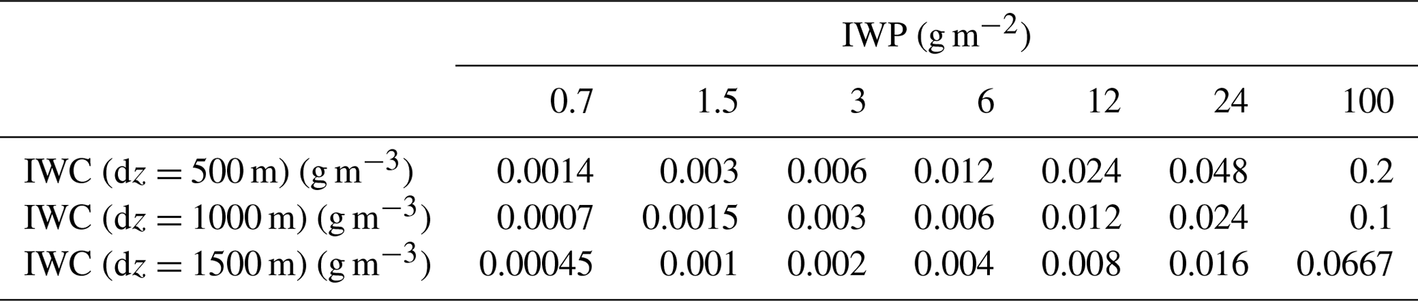
• Cloud geometric thickness dz is set to 1000 m. That represents a contrail after approximately 30 min lifetime (Freudenthaler et al., 1995) and an average cirrus or aged contrail, as confirmed by climatologies from lidar (Noël and Haeffelin, 2007; Iwabuchi et al., 2012) and satellite observations, for example, by Sassen and Campbell (2001). During the cloud lifetime the ice crystals might grow due to supersaturation and WV deposition and start to sediment. Sedimentation lowers the cloud base altitude and increases dz. Meerkötter et al. (1999) reported that variations in dz have only a minor impact on the cloud RE. However, to estimate the effect of varying dz, a dedicated sensitivity study on dz was performed for a sub-set of the parameter range and dz of 500, 1000, and 1500 m. To investigate the effect of variations in dz on solar, TIR, and net RE, a separate sensitivity study for a sub-set of the full parameter space is performed with dz of 500 and 1500 m, while keeping the total ice water path (IWP) constant and, thus, the solar cloud optical thickness τ_ice constant. The total IWP and the scaled IWC are provided in Table 2. τ_ice can be approximated by

  $$\begin{array}{}\text{(10)}& \begin{array}{rl}{\mathit{\tau }}_{\mathrm{ice}}& ={\displaystyle \frac{\mathrm{3}\cdot Q_{\mathrm{e}}\cdot \mathrm{IWC}\cdot \mathrm{d}z}{\mathrm{4}\cdot {\mathit{\rho }}_{\mathrm{ice}}\cdot r_{\mathrm{eff}}}}={\displaystyle \frac{\mathrm{3}\cdot Q_{\mathrm{e}}\cdot \mathrm{IWP}}{\mathrm{4}\cdot {\mathit{\rho }}_{\mathrm{ice}}\cdot r_{\mathrm{eff}}}}\\ & ={\displaystyle \frac{\mathrm{3}\cdot \mathrm{IWP}}{\mathrm{2}\cdot {\mathit{\rho }}_{\mathrm{ice}}\cdot r_{\mathrm{eff}}}},\end{array}\end{array}$$

  with the density of ice ρ_ice=917 kg m⁻³, and Q_e≈2 as the average solar extinction efficiency factor of ice crystals (Horváth and Davies, 2007; Wang et al., 2019). It has to be noted that Eq. (10) is only applicable for the solar wavelength range.

• The parameter sensitivity study is complemented by investigating the influence of a second cloud layer. The second cloud layer is implemented as a stratiform, low-level liquid water cloud, with a constant cloud-top altitude z_liq,CT at 1500 m and a geometric thickness of 500 m. The altitude of 1500 m was selected as a compromise between typical conditions of low-level stratiform clouds in the sub-Arctic, mid-latitude, and tropical regions. McFarquhar et al. (2007) and van Diedenhoven et al. (2009) found $z_{\mathrm{liq},\mathrm{CT}}=\mathrm{1000}\mathrm{m}$ for Arctic clouds. Slightly higher z_liq,CT between 1000 and 1500 m are found in the mid-latitudes (Rémillard et al., 2012; Muhlbauer et al., 2014). Low-level clouds in the tropics also range between 500 and 1700 m, even though some cloud tops can reach up to 2000 m (Medeiros et al., 2010; Stevens et al., 2016). Fixing z_liq,CT at 1500 m leads to liquid cloud-top temperature T_liq of 278.5 and 290.7 K for the mid-latitude and tropical profile, respectively. In the sub-Arctic profile, however, T_liq reaches 257.2 K (−15.95 K), which is below freezing and implies a super-cooled liquid water cloud. This agrees with observations from Hogan et al. (2004) and Hu et al. (2010), who found that the majority of clouds in the Arctic (≈ 70 %) are characterized by super-cooled droplets at the cloud top. Furthermore, 95 % of the observed clouds that have a T_liq between −15 and 0 ^∘C have super-cooled droplets at the top. The cloud optical thickness τ_liq at 550 nm wavelength of the liquid water cloud is varied between 0 and 20. Within the RT simulations, the optical properties of liquid water clouds are represented by precalculated Mie tables (Mie, 1908; van de Hulst, 1981).

Table 2 Ice water path (IWP; in g m⁻²) and ice water content (IWC; in g m⁻³) for the reference, with dz=1000 m, and the two additional clouds, with dz of 500 and 1500 m.

(Stamnes et al., 1988; Buras et al., 2011)Kurucz (1994)(Gasteiger et al., 2014)Yang et al. (2013)

Table 3 Basic model configuration and selected settings.

Table 4 Simulated parameter space.

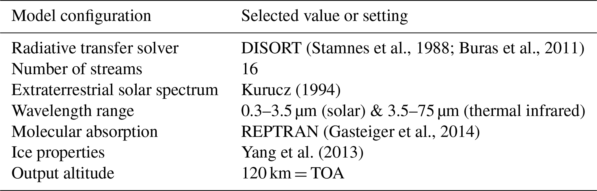
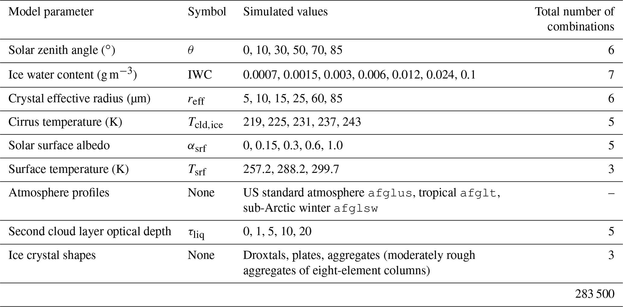
An overview of the model configuration is given in Table 3 and the input parameter space is listed in Table 4. An example libRadtran input file is provided as Supplement.

Table 5 List of variables that are provided in the NetCDF. The output is provided at top of atmosphere located at 120 km altitude.

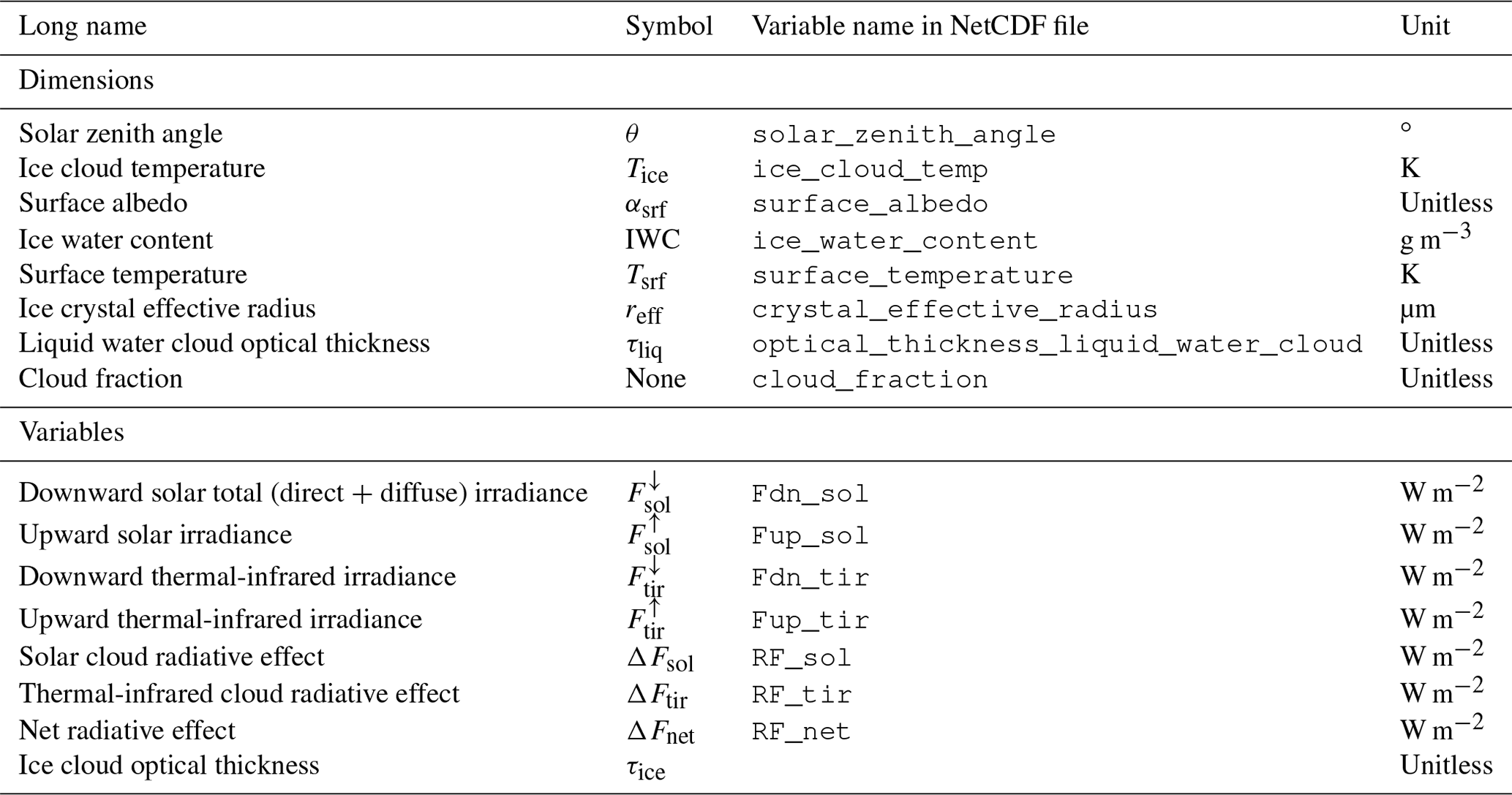
For each of the three simulated ice crystal shapes, a NetCDF file is provided (Wolf et al., 2023). The files include ice cloud optical thickness τ_ice, the simulated upward and downward irradiances F at TOA with 120 km (with and without the presence of the ice cloud), and the calculated ice cloud radiative effect ΔF (solar, TIR, and net). The available cloudy and cloud-free irradiances further allow us to calculate the cirrus RE by scaling the “cloudy” RE with the required cloud cover. An overview of all variables provided in the NetCDF files is given in Table 5. The data set allows the user to extract ΔF values for their parameter combinations, instead of running costly RT simulations. The lookup table could in fact be coupled with models of any complexity, as long as they simulate the dimensions of the data set, namely solar zenith angle, ice cloud temperature, surface albedo, ice water content, surface temperature, ice crystal effective radius, and liquid water cloud optical thickness.

The simulations base on three relative humidity profiles, which were selected to represent sub-Arctic, mid-latitude, and tropical conditions. An estimation of the RE variability due to variations in the RH profile showed an effect of less than 1 % for ΔF_sol but can range up to 4 % for ΔF_tir and 8 % for ΔF_net, especially for the warm and moist tropical profile. These variations have to be considered when using the data set. We further emphasizes that the simulations are performed with a 1D RT solver, i.e., plane-parallel clouds that neglect 3D scattering and horizontal photon transport (Gounou and Hogan, 2007).

2.3 Relationship between effective radius, ice water content, crystal number concentration, and cloud optical thickness

The liquid water content (LWC) of a liquid water cloud can be obtained by

$$\begin{array}{}\text{(11)}& \mathrm{LWC}={\displaystyle \frac{\mathrm{4}}{\mathrm{3}}}\cdot \mathit{\pi }\cdot {\mathit{\rho }}_{\mathrm{liq}}\cdot \underset{\mathrm{0}}{\overset{\mathrm{\infty }}{\int }}n\left(r\right)\cdot r^{\mathrm{3}}\cdot \mathrm{d}r,\end{array}$$

with ρ_liq=1000 kg m⁻³ as the density of liquid water, r as the radius, and n(r) as the number of droplets with size r. Equation (11) assumes spherical ice crystals, so it might be valid for droxtals, which are almost spherical ice crystals, but it is invalid for other ice crystal shapes. To obtain the particle number concentration N_ice for non-spherical crystals, appropriate power law–mass–dimension relations are needed. Here we employ Eq. (29) from Mitchell et al. (2006) but modify the notation to be consistent with the previous equations from the present study. Equation (29) from Mitchell et al. (2006) is then given as

$$\begin{array}{}\text{(12)}& \mathrm{IWC}={\displaystyle \frac{\mathit{\alpha }\cdot \mathrm{\Gamma }(\mathit{\beta }+\mathit{\mu }+\mathrm{1})\cdot N_{\mathrm{ice}}}{\mathrm{\Gamma }(\mathit{\mu }+\mathrm{1})\cdot {\mathrm{\Lambda }}^{\mathit{\beta }}}},\end{array}$$

with Γ being the result of the numerically solved gamma function. The constants α and β are the prefactor and the power in the mass–dimensional relationship, respectively. They are related by

$$\begin{array}{}\text{(13)}& m=\mathit{\alpha }\cdot D^{\mathit{\beta }},\end{array}$$

with m as the mass of the ice crystal, and D as the maximum dimension of the ice crystal. Both constants depend on the ice crystal shape and are, for example, listed in Mitchell (1996). Using Eq. (12) and assuming an exponential PSD with the special case μ=0 and $\mathrm{\Lambda }=\frac{\mathrm{3}}{r_{\mathrm{e}}}$ (Deirmendjian, 1962; Petty and Huang, 2011) finally leads to

$$\begin{array}{}\text{(14)}& N_{\mathrm{ice}}={\displaystyle \frac{{\mathrm{3}}^{\mathit{\beta }}\cdot \mathrm{IWC}}{\mathit{\alpha }\cdot \mathrm{\Gamma }(\mathit{\beta }+\mathrm{1})\cdot r_{\mathrm{e}}^{\mathit{\beta }}}}.\end{array}$$

Therefore, N_ice is proportional to $\frac{\mathrm{IWC}}{r_{\mathrm{e}}^{\mathit{\beta }}}$, with β at around 2 for aggregates, 2.4 for hexagonal-plates, and 3 for almost spherical droxtals (Mitchell, 1996).

2.4 Approximation of radiative transfer in the thermal infrared

Radiation in the TIR is primarily of terrestrial origin (Glickman, 2000). Therefore, the TIR irradiance at the TOA has only an upward-directed component $F^{\uparrow ,\mathrm{TIR}}$, while the downward component $F^{\downarrow ,\mathrm{TIR}}$ is essentially zero. The magnitude of $F^{\uparrow ,\mathrm{TIR}}$ is primarily driven by the cloud absorption optical depth, the surface temperature T_srf, and the (ice) cloud temperature T_cld,ice or ice cloud altitude z_ice (Corti and Peter, 2009). Assuming the Earth's surface is a blackbody, the outgoing $F_{\mathrm{TIR}}^{\uparrow }$ at TOA could be calculated, in a first-order approximation, by the Stefan–Boltzmann law

$$\begin{array}{}\text{(15)}& F_{\mathrm{cf}}^{\uparrow }=\mathit{\sigma }\cdot \mathit{ϵ}\cdot T^{\mathrm{4}},\end{array}$$

which is obtained by integrating the Planck function over all wavelengths and 2π of a hemispheric solid angle. In Eq. (15), the Stefan–Boltzmann-constant is represented by $\mathit{\sigma }=\mathrm{5.67}\times {\mathrm{10}}^{-\mathrm{8}}$ W m⁻² K⁻⁴ and the emissivity ϵ=1 of a blackbody. In reality, however, the Earth acts as a graybody (ϵ≠1), and the surrounding atmosphere must be taken into account.

Absorption of radiation in the atmosphere in the TIR wavelength range depends on the wavelength and atmospheric composition. The primary components that control absorption are water vapor and carbon dioxide (CO₂) (Liou, 1992). While CO₂ is well-mixed and thus approximately constant in space and time, WV is highly variable. Furthermore, the amount of WV is linked to the temperature in the AP via the Clausius–Clapeyron equation (Corti and Peter, 2009). The lowermost values of the AP are also influenced by T_srf. Due to these interactions, Corti and Peter (2009) developed a model to estimate TIR irradiances and the resulting CRE. The model was derived by fitting RT simulations, which cover a wide range of environmental conditions, to Eq. (15), which leads to

$$\begin{array}{}\text{(16)}& F_{\mathrm{cf}}^{\uparrow \ast }\approx {\mathit{\sigma }}^{\ast }\cdot \mathit{ϵ}\cdot T_{\mathrm{srf}}^{k^{\ast }},\end{array}$$

with ${\mathit{\sigma }}^{\ast }=\mathrm{1.607}\times {\mathrm{10}}^{-\mathrm{4}}$ W m⁻² K^−2.528 and $k^{\ast }=\mathrm{2.528}$. $F_{\mathrm{cf}}^{\uparrow \ast }$ represents the surface emission with T_srf and atmospheric absorption.

Clouds in the atmosphere can be approximated by semi-transparent blackbodies that partly absorb and re-emit radiation, according the Stefan–Boltzmann law. The emissivity ϵ of a cloud depends on τ, which in turn depends on the wavelength (Stephens et al., 1990). $F_{\mathrm{TIR}}^{\uparrow }$ in the cloudy case can be estimated with

$$\begin{array}{}\text{(17)}& F_{\mathrm{TIR}}^{\uparrow }=\left(\mathrm{1}-{\mathit{ϵ}}^{\ast }\right)\cdot {\mathit{\sigma }}^{\ast }\cdot T_{\mathrm{srf}}^{k^{\ast }}+{\mathit{ϵ}}^{\ast }\cdot {\mathit{\sigma }}^{\ast }\cdot T_{\mathrm{cld}}^{k^{\ast }},\end{array}$$

with σ^∗ and k^∗ for cloud-free conditions. ϵ can be approximated by

$$\begin{array}{}\text{(18)}& \mathit{ϵ}\approx \mathrm{1}-\exp -\mathit{\delta }\cdot \mathit{\tau },\end{array}$$

where $\mathit{\delta }=D\cdot (\mathrm{1}=\stackrel{\mathrm{̃}}{\mathit{\omega }})$ and D≈1.66, relying on the zero-scattering assumption (Stephens et al., 1990), and an effective emissivity ϵ^∗ that is also derived from their RT simulations. Finally, the TIR RE of a cloud above a surface can be approximated with

$$\begin{array}{}\text{(19)}& \begin{array}{rl}\mathrm{\Delta }{F}_{\mathrm{tir}}& =F_{\mathrm{TIR},\mathrm{c}}-F_{\mathrm{TIR},\mathrm{cf}}\\ & \approx {\mathit{\sigma }}^{\ast }\left(T_{\mathrm{srf}}^{k^{\ast }}-T_{\mathrm{cld}}^{k^{\ast }}\right)\cdot \left(\mathrm{1}-\exp \left(-{\mathit{\delta }}^{\ast }\cdot \mathit{\tau }\right)\right),\end{array}\end{array}$$

with ${\mathit{\delta }}^{\ast }=\mathrm{0.75}$. It follows from Eq. (19) that the forcing of a cloud, with constant τ, is proportional to the temperature difference between cloud and surface.

3 Results

We first provide an overview of how r_eff and IWC determine the cloud optical and microphysical properties. Figure 1a–d illustrate the dependence of N_ice and τ_ice as a function of r_eff and IWC. N_ice is approximated by Eq. (14), assuming droxtals (almost spherical ice crystals), a mono-disperse particle size distribution, and a cloud geometric thickness dz of 1000 m. The ice cloud optical thickness τ_ice at 550 nm wavelength is directly obtained from the libRadtran verbose output, using optical properties of droxtals. The largest N_ice values result from the smallest ice crystal sizes (r_eff<10 µm), particularly in combination with large IWC (Fig. 1a). For combinations of small r_eff<15 µm and large IWC, N_ice is most sensitive to r_eff, which is indicated by the narrowing contour lines that align along the x axis. For a constant r_eff of 5 µm, the estimated N_ice ranges from 1 to over 80 cm⁻³. Such concentrations of N_ice>80 cm⁻³ are rarely observed in natural cirrus, though they can occur in very young contrails and contrail-induced cirrus (Krämer et al., 2016). Generally, smaller N_ice and a reduced sensitivity to r_eff and IWC is found for r_eff>20 µm, where N_ice mostly ranges below 10 cm⁻³.

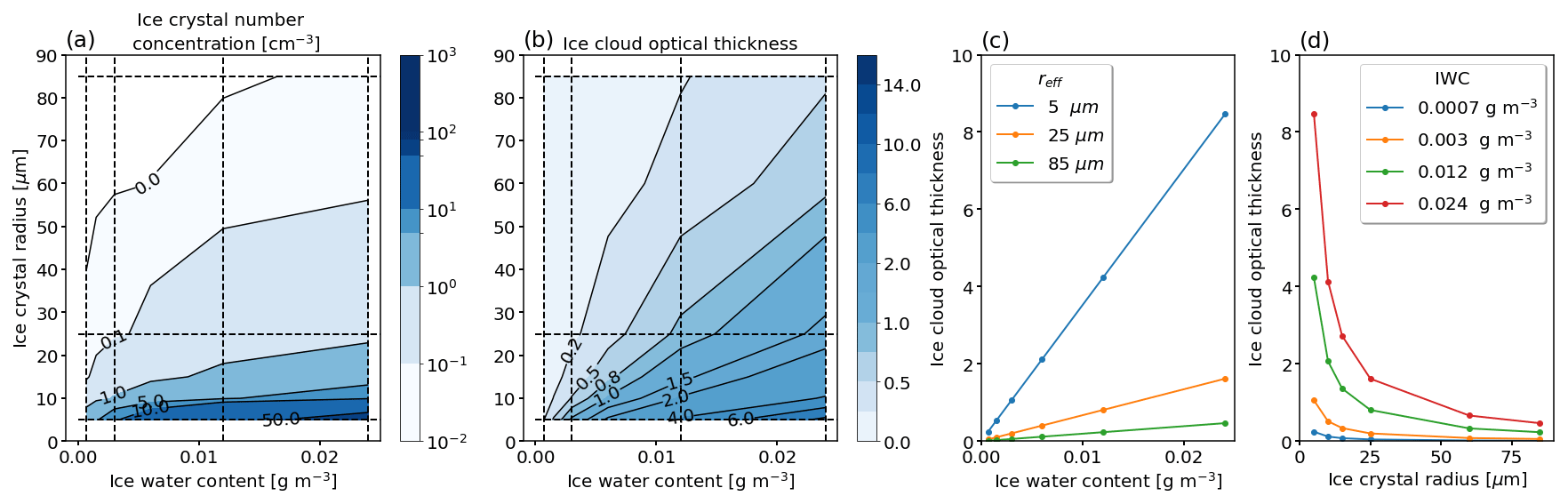
Figure 1 (a–b) Calculated ice crystal number concentration N_ice (in cm⁻³) and simulated cloud optical thickness τ_ice at 550 nm wavelength as a function of ice water content IWC (in g m⁻³) and effective crystal radius r_eff (in µm), assuming droxtals. A cloud geometric thickness dz of 1000 m is selected. (c–d) Cross sections along lines of constant r_eff or IWC that are indicated as dashed lines in panels (a) and (b), respectively.

The inherent dependencies of N_ice presented in Fig. 1a are also found in the distribution of the ice cloud optical thickness τ_ice at 550 nm, as shown in Fig. 1b. Following the lines of constant r_eff (Fig. 1c), the increase in IWC corresponds to a linear increase in N_ice and, therefore, to a gain in the total scattering and absorption particle cross sections. The absorption of radiation by liquid water and ice (as characterized by the complex refractive index) at 550 nm wavelength is weak, and therefore, scattering dominates τ_ice. Alternatively, going along the lines of constant IWC towards larger r_eff leads to a decrease in N_ice and a related decrease in the total scattering particle cross section (cloud albedo effect; Fig. 1d). This effect is most effective for larger IWC (optically thick clouds) and is less pronounced for clouds with smaller IWC.

To reduce the multi-dimensionality, for each of the eight parameters, a reference is defined by selecting either the minimum or maximum value from the parameter space. The reference parameters are selected to highlight the upper or lower range of each parameter and the spanned variation and to define the reference for the fixed parameters. The reference parameters are given by θ=0^∘, $T_{\mathrm{cld},\mathrm{ice}}=\mathrm{219}$ K, α_srf=0, T_srf=299.7 K, r_eff=85 µm, and τ_liq=0 (no liquid water cloud). For IWC, we use an intermediate value of 0.024 g m⁻³ because, together with a dz of 1000 m and an r_eff of 85 µm, this leads to a τ_ice of 0.46 at 550 nm wavelength, which is representative of contrails and young cirrus (Iwabuchi et al., 2012). Otherwise, electing the minimum or maximum IWC in combination with r_eff of 85 µm would lead to high or low τ_ice values that are not representative of contrails. For the ice crystal shape, we select aggregates as the reference. We particularly emphasize that the defined references are not representative of any particular cloud situation but are a useful point of comparison to assess the impact of a given parameter on the diversity of cloud RE.

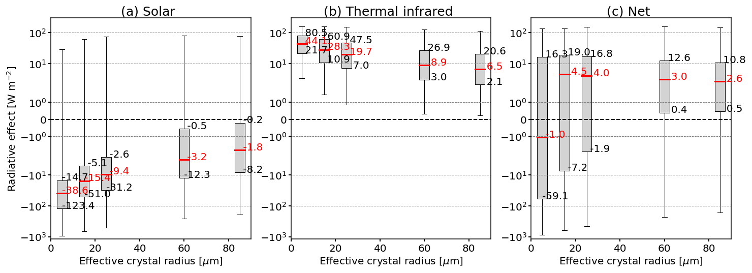
Using the defined reference, Fig. 2a–c show solar, TIR, and net ΔF, respectively (similar to Meerkötter et al., 1999). First, the influence of the variations in θ is investigated in order to sample the diurnal cycle and its variation as a function of latitude. For all Sun geometries, ΔF_sol is negative, and therefore, the cirrus has a cooling effect in the solar spectrum on the atmosphere–surface system. ΔF_sol intensifies (i.e., becomes more negative) with increasing θ as the length of the optical path through the cloud, $s=\mathrm{\Delta }z/\cos \mathit{\theta }$, increases, which is accompanied by enhanced scattering (and thus upward-directed scattering) of the incoming radiation (Wendisch et al., 2005). In addition, a lower fraction of the incident radiation is scattered towards the surface but scattered upward to space. This is due to the strong forward peak in the ice crystal phase function 𝒫 that decreases sharply for Θ>10^∘ (see Fig. D1 in the Appendix). An exception appears for θ of 85^∘, where ΔF_sol is the smallest. Variations in θ lead to ΔF_sol between −55.9 and −27.5 W m⁻². As expected, ΔF_tir is unaffected by the Sun position, with a constant ΔF_tir = 46.0 W m⁻². The resulting sensitivity of ΔF_net is driven by ΔF_sol, with ΔF_net between −9.9 and 18.5 W m⁻². During nighttime, there is no contribution from ΔF_sol, leading to a constant positive ΔF_net = 46.0 W m⁻² (leading to a warming).

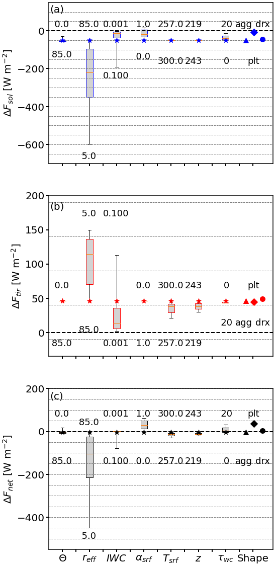
Figure 2 (a–c) Box-and-whisker plot of solar, TIR, and net ΔF (in W m⁻²), due to the variation in the parameters indicated on the x axis. The boxes represent the 25th and 75th percentiles, while the whiskers indicate the minimum and maximum values. Median values are given in each box by horizontal orange lines. The stars indicate the reference with the solar zenith angle θ=0^∘, effective radius r_eff = 85 µm, ice water content IWC = 0.024 g m⁻³, surface albedo α_srf=0, surface temperature T_srf=299.7 K, ice cloud temperature $T_{\mathrm{cld},\mathrm{ice}}=\mathrm{219}$ K, and liquid water cloud optical thickness τ_liq=0. Minimum and maximum values of the parameter ranges are given by the numbers. The plot idea has been adapted from Meerkötter et al. (1999).

As expected, variations in r_eff have the largest effect on the solar, TIR, and net ΔF, as N_ice relates to r_eff by the power of −β, which depends on the ice crystal shape (see Sect. 2.3 and Eq. 14). Increasing r_eff from 5 to 85 µm leads to ΔF_sol between −599.5 and −50.2 W m⁻². The distribution of ΔF_tir has a minimum and maximum of 46.0 and 149.8 W m⁻², respectively. ΔF_sol dominates ΔF_tir and results in values of ΔF_net ranging from −449.8 to −4.2 W m⁻².

Variations in IWC affect the solar, TIR, and net ΔF. Generally, an increase in IWC (increase in τ_ice for fixed r_eff) enhances total scattering and absorption particle cross sections and, therefore, intensifies the cooling in the solar (more negative ΔF and cloud albedo effect) and the TIR heating (more positive ΔF). ΔF_sol ranges from −191.1 to −1.5 W m⁻², with $\mathrm{\Delta }{F}_{\mathrm{sol}}=-\mathrm{50.2}$ W m⁻² obtained for the reference IWC. The distribution of ΔF_tir spans values between 1.8 and 112.7 W m⁻², leading to ΔF_net from −78.4 to 1.1 W m⁻². The ΔF values given above correspond to a varying IWC and assume r_eff=85 µm. For smaller r_eff, ΔF increases and thus increases the range of solar, TIR, and net ΔF. In addition, the IWC becomes dominant over r_eff in Fig. 2, when selecting a reference with smaller r_eff.

Variations in α_srf impact only the solar spectrum, as expected, with ΔF_sol between −50.2 and 15.4 W m⁻². The most negative RE appears over non-reflective surfaces and decreases with increasing α_srf, due to the decrease in contrast between the surface and the cirrus. In cases where α_srf exceeds the cloud albedo, ΔF_sol becomes positive. For the optical thin reference, this is the case over a fully sea-ice-covered area, with α_srf≈1. The TIR component remains almost unaffected, with ΔF_tir between 39.5 and 46 W m⁻². Together with the decreasing cooling effect in the solar range, the warming in the TIR mostly dominates and leads to ΔF_net ranging between −4.2 and 55.0 W m⁻².

The influence of a varying surface temperature T_srf or cirrus temperature T_cld,ice (related to cloud base altitude) is investigated for a cloud scenario with a solar surface albedo α_srf set to 0. Varying surface temperature T_srf or cirrus temperature T_cld,ice (related to cloud base altitude), ΔF_sol remains almost constant, with a minimum and maximum ΔF_sol for both parameters of −50.2 and −49.2 W m⁻², respectively. These small differences are due to the changes in molecular absorption, which results from the variations in the relative humidity profile, as the profile depends on the selected T_srf. A noticeable effect is found for ΔF_tir, which is impacted by variations in T_cld,ice and T_srf. While decreasing T_cld,ice from 243 to 219 K lowers ΔF_tir from 46 to 29.9 W m⁻², a decrease in T_srf from 300 to 257 K reduces ΔF_tir from 46 to 20.8 W m⁻². Consequently, ΔF_tir determines the response of the resulting ΔF_net, which spans from −4.2 to −19.4 W m⁻² for T_cld,ice and −28.7 to −4.2 W m⁻² for T_srf. The greater influence of T_srf on ΔF_tir and ΔF_net is explained simply by the greater variation in the input.

A second cloud layer is considered by inserting a liquid water cloud with a cloud-top altitude of z_base=1500 m and a geometric thickness of dz=500 m. Figure 2 shows that this second cloud influences both components of ΔF_sol and ΔF_tir. Generally speaking, the liquid water cloud enhances the fraction of solar, upward-directed radiation compared to a dark surface. With increasing τ_liq (increase in LWC), α_cld,ice exceeds α_srf, which lowers the albedo contrast between the ice cloud and the surface for most of the parameter combinations. This minimizes solar RE and leads to a minimum of −51.1 W m⁻² and a maximum of −11.6 W m⁻². For the TIR part, the increase in the LWC masks the influence of the underlying surface by absorbing the upward TIR radiation from the surface and re-emitting radiation at the liquid water cloud temperature. This leads to ΔF_tir between 43.2 and 46.0 W m⁻². The resulting ΔF_net is characterized by a minimum and maximum of −6.5 and 31.6 W m⁻², which is primarily impacted by the solar component.

The parameter study is complemented by investigating the effect of prescribing three different ice crystal shapes. The variation in ΔF_sol due to the transition from almost spherical (droxtals) to non-spherical crystals (aggregates) leads to a relative change in ΔF_sol that is, in terms of RE, comparable to a variation in θ. The strongest cooling effect (negative ΔF_sol) is found for aggregates with −50.2 W m⁻² and decreases for droxtals and plates to −44.3 and −8.6 W m⁻², respectively. The ice crystal shape also impacts ΔF_tir. Aggregates lead to ΔF_tir of 46 W m⁻², while plates and droxtals can cause a ΔF_tir of 44.5 and 48.9 W m⁻², respectively. Consequently, the largest ΔF_net with 35.8 W m⁻² is found for plates and followed, in decreasing order, by droxtals and aggregates, with 4.5 and −4.2 W m⁻², respectively. As mentioned in the Introduction, the uncertainty in the ice crystal shape causes uncertainties in the calculated ΔF. Nevertheless, using three different ice crystal shapes for the irradiance simulations shows that the shape-specific scattering properties are of lesser importance compared to other parameters like the ice crystal size (distribution), the IWC, or surface properties.

The presented analysis of solar, TIR, and net ΔF sensitivity on the selected input parameters generally agrees with the results from Meerkötter et al. (1999). We found differences in the importance of the parameters, which are explained by the fact that our simulations span a larger and different parameter range, for example, in r_eff, IWC, and T_srf. Selecting cloud parameters (θ=30^∘, $T_{\mathrm{cld},\mathrm{ice}}=\mathrm{231}\mathrm{K}$, α_srf=0.15, T_srf=288 K, r_eff=10 µm, and τ_liq=0), whether using case A in Meerkötter et al. (1999), we find that the IWC becomes the driving parameter, which then agrees with the results from Meerkötter et al. (1999). However, a more quantitative comparison between Meerkötter et al. (1999) is difficult, as the parameters that best match are not identical. Even by choosing similar cloud parameters, by matching the IWP and selecting r_eff to yield τ_ice ≈ 0.52, the simulated clouds and cloud case A from Meerkötter et al. (1999) differ in dz, which impacts ΔF_sol and ΔF_tir with a different intensity.

It is further emphasized that the presented ΔF_net is representative of daytime situations only, when the Sun is above the horizon. In the absence of solar illumination during nighttime, the net effect is entirely determined by and equal to ΔF_tir, which is positive (warming effect) in all simulation cases. Accordingly, all simulated cloud cases do have a net warming effect at night. For a more in-depth analysis, the subsequent plots focus on the impact of each individual parameter.

3.1 Sensitivity on ice crystal shape

One difficulty of RT simulations in ice clouds is the uncertainty about the dominating ice crystal shape, which is commonly unknown, and therefore, a general ice crystal shape has to be assumed (Kahnert et al., 2008). Scattering and absorption by an ice crystal is characterized by its orientation, complex refractive index of ice, the wavelength of the incident light, shape, size, and the resulting asymmetry parameter. The asymmetry parameter is a measure of the asymmetry of the phase function 𝒫 between forward and backward scattering (Macke et al., 1998; Fu, 2007). 𝒫 provides the angular distribution of the scattered direction in relation to the incident light. For example, in the case of idealized hexagonal ice crystals and a wavelength below 1.4 µm, the asymmetry parameter is primarily determined by the ice crystal shape $/$ aspect ratio, but for wavelengths larger than 1.4 µm, the asymmetry parameter also depends on the ice crystal size (Fu, 2007; Yang and Fu, 2009; van Diedenhoven et al., 2012). Consequently, the assumption of an ice crystal habit and ice crystal size, with the related aspect ratio, is vital information for the estimation of the ice cloud RE. Furthermore, the ice optical properties by Yang et al. (2010, 2013), which are used for the RT simulations in the present study, based on a coupling of the maximum diameter of the ice crystal and the aspect ratio, with the latter one being different for each crystal shape. This impacts the RT of different ice clouds with varying IWC and r_eff.

Subsequently, the shape effect is quantified using Eq. (20), and relative differences in ΔF are given with respect to crystals with the same r_eff in relation to the ΔF simulated for aggregates.

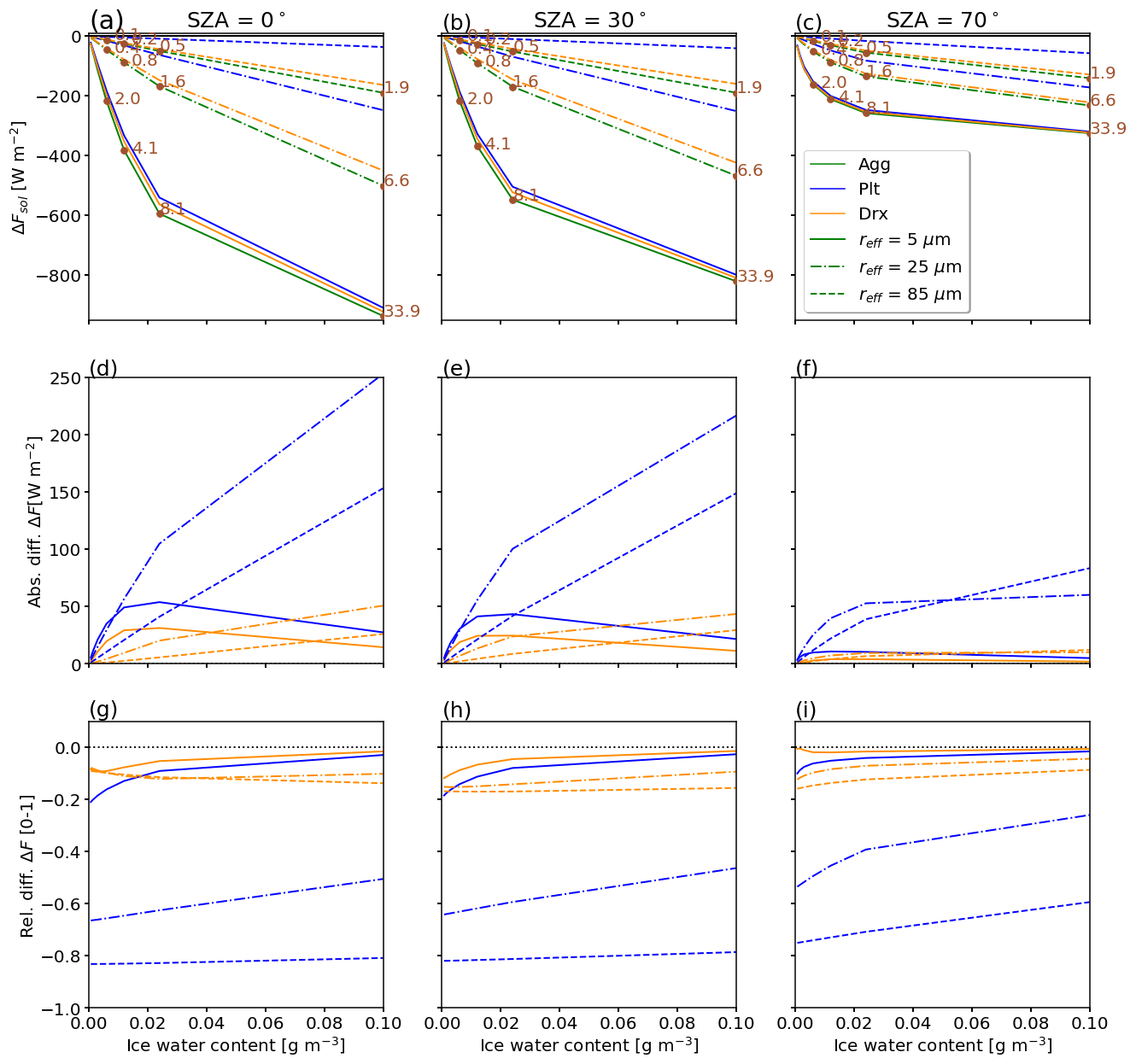
Figure 3 (a–c) Solar radiative effect ΔF_sol (in W m⁻²) as a function of ice water content IWC for three values of the solar zenith angle with θ of 0, 30, and 70^∘. Three ice crystal radii r_eff of 5 (solid), 25 (dash-dotted), and 85 µm (dashed) are indicated. The ice crystal shape is color coded, with the aggregates “Agg”, plates “Plt”, and droxtals “drx” given in green, blue, and orange, respectively. Panels (d)–(f) show the absolute difference and panels (g)–(i) show the relative difference between ΔF_sol of droxtals and plates with respect to aggregates with the same crystal radius. The numbers indicate the optical thickness simulated for the reference that contains ice aggregates.

Figure 3a–c show ΔF_sol as a function of IWC, separated for crystal shape, r_eff, and three selected θ. For simplicity, α_srf and τ_liq are set to zero in this discussion.

The strongest ΔF_sol is found for aggregates (green) with r_eff=5 µm, with the Sun at zenith (θ=0^∘; Fig. 3a). A lower cooling effect in the solar spectrum is found for droxtals (orange) and plates (blue) with the same r_eff. The order of ΔF_sol remains constant for increasing r_eff.

The spread in ΔF_sol across crystal shapes with the same r_eff and IWC can be interpreted as a potential uncertainty in ΔF_sol, due to the ice crystal shape. One has to keep in mind that the differences partially result from deviating crystal size distributions, as these depend on the selected crystal shape. Macke et al. (1998) showed that, in the solar wavelength range, the crystal shape is the main driver, and the actual ice PSD has only a minor effect on ΔF_sol. Nevertheless, Mitchell (2002) and Mitchell et al. (2011) found that the PSD also has a considerable impact on ΔF_tir, leading to differences of up to 48 % in the single-scattering albedo when switching between PSDs.

To quantify the deviations resulting from the ice crystal shape, Fig. 3d–f show the absolute and Fig. 3g–i present the relative differences in ΔF_sol of droxtals and plates with respect to aggregates. For θ=0^∘, the largest absolute deviation is found for plates with r_eff of 25 µm and the highest IWC with an absolute range of up to 250 W m⁻² (r_eff=25 µm, θ=0^∘, τ_ice=6.6), corresponding to a relative difference of 58 %. Relative deviations reach even larger values, e.g., when the cloud is optically thinner and ΔF_sol becomes smaller. In the case of plates, the relative deviations range from −20 % (r_eff=5 µm) to −82 % (r_eff=85 µm). The large absolute and relative deviations between plates and aggregates in ΔF_sol and later ΔF_net appear because plates are characterized by the smallest reflectance and absorption efficiency (Key et al., 2002; Yang et al., 2005). The absolute differences among droxtals and aggregates are smaller. With increasing IWC, the absolute ranges quickly reach a maximum of 27 W m⁻² at an IWC of 0.024 g m⁻³ and decrease towards the largest IWC. The associated relative deviations are also smaller compared to plates, ranging between −3 % (r_eff=5 µm) and −18 % (r_eff=85 µm).

Another characteristic of the absolute range of ΔF_sol is the steep slope for θ=0^∘ over the entire range of IWC. For illumination geometries with the Sun closer to the horizon, particularly θ=70^∘, the behavior of absolute range in ΔF_sol is characterized by a rapid increase and convergence towards a maximum. At a certain IWC and related τ_ice, the slant optical path and cloud–radiation interactions are dominated by multiple scattering that suppresses single-scattering effects of individual ice crystal shape and, hence, reducing the absolute and relative difference resulting from the choice of the ice crystal shape. This is supported by earlier observations and simulations, for example, by Wendisch et al. (2005), who showed that for large θ and multiple-scattering the shape effect becomes less prominent.

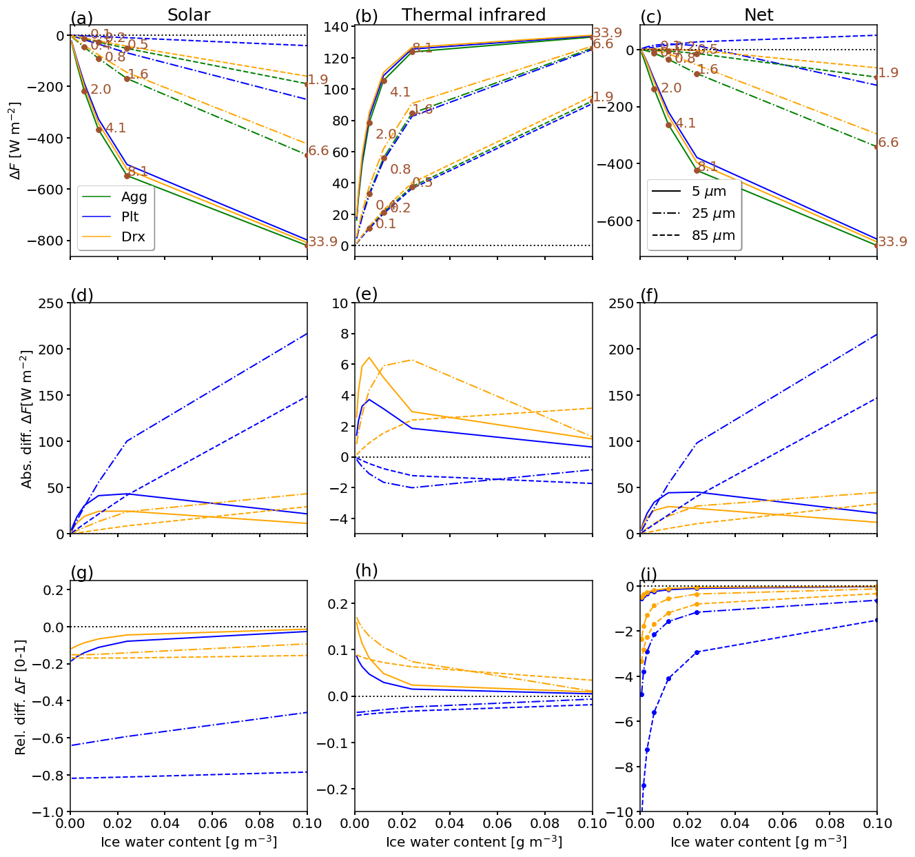
Figure 4 Same as Fig. 3 but for solar zenith angle θ=30^∘. ΔF_sol (a, d, g), ΔF_tir (b, e, h), and ΔF_net (c, f, i).

Next, we consider the solar, TIR, and net ΔF at θ=30^∘ (Fig. 4). The leftmost column for ΔF_sol is identical to the middle column in Fig. 3. In the TIR, the largest ΔF_tir is generally found for smallest crystals (5 µm) and highest IWC in decreasing order from droxtals, plates, and aggregates. With increasing crystal size, the order changes to droxtal, aggregates, and plates, and the absolute values of ΔF_tir decrease. The largest ΔF_tir range of 130 W m⁻² is found for clouds with IWC between 0.024 and 0.1 g m⁻³ caused by droxtals. For thin clouds with IWC < 0.04 g m⁻³, the largest absolute range R_ΔF,tir of around 6.5 W m⁻² appears for r_eff of 5 and 25 µm, which is shifting towards larger IWC with increasing r_eff and vanishes for the largest crystals with r_eff of 85 µm. The relative differences are the largest for the optically thinnest clouds and decrease with increasing IWC. While droxtals are characterized by relative differences close to 0 % (r_eff=5 µm; IWC = 0.1 g m⁻³) and 18 % (r_eff=25 µm; IWC = 0.007 g m⁻³), plates lead to relative differences between 9 % (r_eff=5 µm; IWC = 0.007 g m⁻³) and −5 % (r_eff=85 µm; IWC 0.007 g m⁻³). The TIR RE of the optically thickest cloud is independent on ice crystal shape, which is addressed to multiple scattering.

For all IWC and r_eff, ΔF_sol is generally larger than ΔF_tir and, therefore, dominates the resulting ΔF_net (Fig. 4c, f). Consequently, ΔF_net and the absolute ranges among the ice crystal shapes follow the distributions from ΔF_sol. The largest relative deviations are found for the optically thinnest clouds, where ΔF_net is generally small. In these cases of optically thin clouds consisting of the smallest crystals (r_eff=5 µm), the relative deviations exceed the relative difference for optically thick clouds with the same crystal size by a factor of 10.

The analysis of all simulations shows that the crystal shape assumption on the cirrus RE is small compared to other parameters, particularly IWC or r_eff (see Fig. 2). However, we found a larger variability in ΔF_sol and the resulting ΔF_net (i.e., whether a contrail has a net warming or cooling effect compared to ΔF_tir). For the defined reference consisting of aggregates, a ΔF_sol value of −50.2 W m⁻² was simulated, while for plates and droxtals, values for ΔF_sol of −8.6 and −44.3 W m⁻² were obtained, respectively. The impact of the crystal shape is less pronounced in the TIR wavelength range, with ΔF_tir of 46, 44.5, and 48.9 W m⁻² for aggregates, plates, and droxtals, respectively. The variation in ΔF_sol propagates into ΔF_net, with −4.2, 35.9, and 4.6 W m⁻² for aggregate, plates, and droxtals, respectively. Based on the presented simulations, we found larger maximum variations in ΔF_sol, ΔF_tir, and ΔF_net of 41.6, 4.4, and 40 W m⁻², respectively, compared to Meerkötter et al. (1999). They found variations in ΔF_sol, ΔF_tir, and ΔF_net of 2, 6, and 7 W m⁻², respectively. The difference is explained by the selected reference (Meerkötter et al., 1999). However, even when selecting cloud parameters similar to the reference cloud of Meerkötter et al. (1999), we still found larger maximum variations in ΔF_sol, ΔF_tir, and ΔF_net of 17.3, 4.2, and 17.9 W m⁻², respectively. This is attributed to the remaining differences among the selected reference values.

3.2 Sensitivity on solar zenith angle and surface albedo

In this section, the impact of each parameter is estimated by fixing one parameter at a time (represented by the x axis), while the others can vary. For example, in case of θ, all simulations, for steps of θ given in Table 4, are extracted from the eight-dimensional (8D) hypercube. The extracted sub-sample, in the example for a specific θ, is used to calculate and visualize the distributions of solar, TIR, and net ΔF. This strategy can be interpreted as a type of sub-sampling, by averaging all unfixed parameters to project ΔF onto the 1D space. The impact of each parameter is further quantified by the minimum and maximum RE. We define the full range of ΔF by

$$\begin{array}{}\text{(20)}& R_{\mathrm{\Delta }F}=max\mathit{\left\{}\mathrm{\Delta }F\mathit{\right\}}-min\mathit{\left\{}\mathrm{\Delta }F\mathit{\right\}},\end{array}$$

with max{ΔF} and min{ΔF} as the maximum and minimum of ΔF across the sub-sampled distributions, respectively. As R_ΔF is susceptible to outliers, we further characterize the width of a distribution by the interquartile range, which is defined as the difference between the 75th (Q_75 %) and 25th (Q_25 %) percentiles of ΔF, as follows:

$$\begin{array}{}\text{(21)}& Q_{\mathrm{\Delta }F}=Q_{\mathrm{75}\mathit{\%}}\left(\mathrm{\Delta }F\right)-Q_{\mathrm{25}\mathit{\%}}\left(\mathrm{\Delta }F\right).\end{array}$$

Variations in θ are caused by the diurnal and seasonal cycle of the Earth or variations along the longitude at a given time.

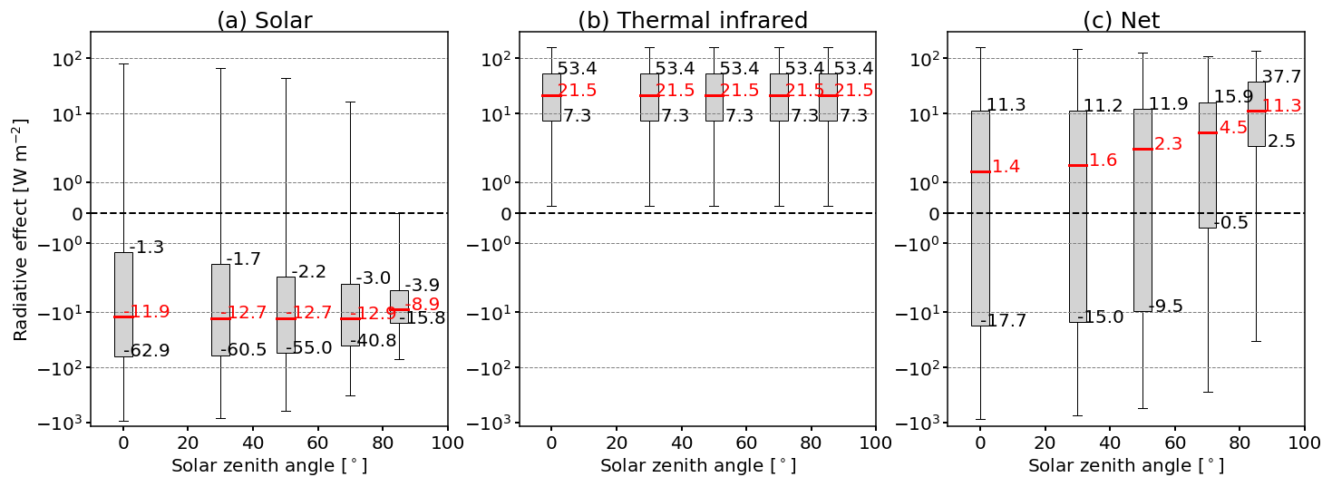
Figure 5 Box plots of (a) solar, (b) TIR, and (c) net ΔF (in W m⁻²) as a function of the solar zenith angle θ. Median values are indicated in red, the 25 %–75 % range is represented by the gray boxes, and the 10 % and 90 % percentiles are given by the whiskers. Red and black numbers indicate the 25th and 75th percentiles and the median value, respectively. Note the logarithmic scale on the y axis.

Figure 5a shows distributions of solar ΔF_sol for θ=0^∘, ranging from −944.5 W m⁻² (high IWC) to 78.0 W m⁻² (high α_srf). For simulated θ<85^∘, the median values range from −11.9 to −12.9 W m⁻², with an intensification of ΔF_sol towards larger θ. At the same time, the upper maxima of ΔF_sol are shifted towards zero, which is a combination of the following three effects: (i) a decreasing downward irradiance at TOA with increasing θ, (ii) an increasing optical path length s through the cloud with increasing θ and the corresponding increase in scattering, and (iii) an increase in upward scattered radiation with increasing θ as the light rays become slanted and a larger fraction of radiation from the forward scattering range is directed upwards. Effects (i) and (ii) compete and are dominated by effect (iii). The combination of effects (i) to (iii) also reduces the interquartile range for larger θ and indicates a reduced influence of the other free parameters on ΔF_sol. However, the smallest ΔF_sol is calculated for θ of 85^∘ and is caused by the reduced sideward scattering of ice crystals.

The value of θ where ΔF_sol is most intense depends on α_srf and is typically located between 50^∘ and 70^∘ (Markowicz and Witek, 2011). The maximum in ΔF_sol and the corresponding θ values are explained by the strong forward-scattering peak of ice crystals and the resulting weak backscattering (Haywood and Shine, 1997; Myhre and Stordal, 2001).

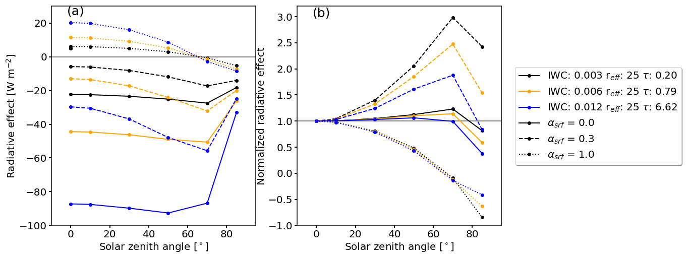
Figure 6 (a) Solar radiative effect ΔF_sol (in W m⁻²) as function of solar zenith angle θ for three ice clouds with cloud optical thickness τ_ice of 0.1, 0.4, and 1.6. The effective radius r_eff (given in units of µm) and the ice water content (IWC; in units of g m⁻³) are shown. The cloud is located over surfaces with a surface albedo α_srf of 0, 0.3, and 1. (b) Same as panel (a) but normalized with ΔF_sol of each case at θ=0^∘.

To further elaborate on the response of ΔF_sol on large θ, Fig. 6a shows ΔF_sol as a function of θ for selected τ_ice and α_srf. For an optically thick cirrus with τ_ice=6.62 located over a surface with α_srf=0 (solid blue curve), the maximum ΔF_sol appears around θ=50^∘. For the same cloud above, a more reflective surface with α_srf=0.3 (dashed blue curve) the maximum is shifted towards θ=70^∘. Further increasing α_srf to 1 (dotted blue curve), solar cooling turns into a heating, and the strongest solar cooling is found for the largest θ. Figure 6a also shows that the shift in the absolute maximum ΔF_sol is most pronounced for optically thicker clouds. However, the largest relative change in ΔF_sol by varying θ appears for optically thin clouds (Coakley and Chylek, 1975).

Figure 6b shows ΔF_sol normalized with the respective ΔF_sol at θ = 0^∘. The sensitivity of normalized ΔF_sol on θ is most pronounced for optically thin clouds, with τ_ice=0.2 over a moderately reflective surface (α_srf=0.3; dashed black). For this combination, ΔF_sol at θ=70^∘ is a factor of 3 larger compared to a Sun overhead (θ=0^∘). The same cloud over a non-reflective surface (α_srf=0) reduces the sensitivity leading to a factor of 1.2 in relation to ΔF_sol at θ=0^∘ (solid black). A similar pattern but with a generally reduced sensitivity is found for the optically thicker cloud case, with τ_ice=6.62. In this case, ΔF_sol is larger by a factor of 1.05 at θ=50^∘ (solid blue) and larger by a factor of 1.7 at θ=70^∘ (dashed blue) with respect to the Sun at θ=0^∘. The large sensitivity for optically thin clouds is explained by the dominance of single scattering, where scattering is strongly dependent on the value of the 𝒫 at a given scattering angle. When the cloud becomes optically thicker, multiple-scattering processes start to dominate the RT, and 𝒫 is averaged over a range of scattering angles, thus reducing the sensitivity on θ. However, while the sensitivity might be largest for optically thin clouds, the absolute ΔF_sol of optically thin clouds is small compared to clouds with higher τ_ice.

Figure 5b shows that ΔF_tir is unaffected by θ, leading to a constant median ΔF_tir of 21.5 W m⁻². The highest positive values of ΔF_tir (strongest warming effect) are found for clouds with maximal IWC. The resulting ΔF_net, shown in Fig. 5c, is dominated by a warming in the TIR that leads to median ΔF_net between 1.4 and 11.3 W m⁻², with a minimum of ΔF_net of −872.8 W m⁻² and maximum of 160.1 W m⁻². With increasing θ, ΔF_net increases. This is caused by the shift in the lower minima of ΔF_sol towards zero, which indicates that a larger fraction of the simulations has a reduced solar cooling effect, and thus, the fraction of simulations with a positive ΔF_net (net warming) increases. The reduced variability in ΔF_sol with increasing θ propagates into the distribution and variability in ΔF_net.

Figure 7 Same as Fig. 5 but as a function of the surface albedo α_srf.

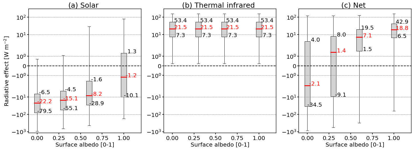
The influence of the underlying surface is shown in Fig. 7. For α_srf=0, the surface absorbs the entire incident solar radiation creating the largest contrast between α_srf and the cloud albedo α_cld. When the surface is fully absorbing (α_srf=0), almost all simulated cloud combinations are characterized by a cooling in the solar range, with ΔF_sol ranging from −944.5 to 80 W m⁻². The cooling is reduced when the surface becomes more reflective and the contrast between surface and cloud is reduced, which shifts the distributions and their medians towards positive ΔF_sol. With α_srf approaching 0.66, around 25 % of the parameter combinations lead to a solar heating. This becomes even more pronounced towards α_srf=1, where around 50 % of the simulations yield a warming effect in the solar range. ΔF_tir is unaffected by changes in α_srf, as expected, and remains constant for all α_srf with a median at 21.5 W m⁻². The resulting ΔF_net is dominated by a net warming effect, indicated by mostly positive median values ranging from 1.4 W m⁻² (α_srf=0.25) to 18.8 W m⁻² (α_srf=1). An exception is α_srf=0, where more than 50 % of the simulations lead to a net cooling, with a median ΔF_net at −2.1 W m⁻².

3.3 Sensitivity on ice water content and ice crystal radius

As presented in Fig. 2, the IWC is the second most influencing factor that controls ΔF. For a constant crystal number concentration, the increase in IWC leads to an increase in r_eff and the total particle scattering and absorption cross sections. This enhances the scattering and absorption along the optical path s though the cloud.

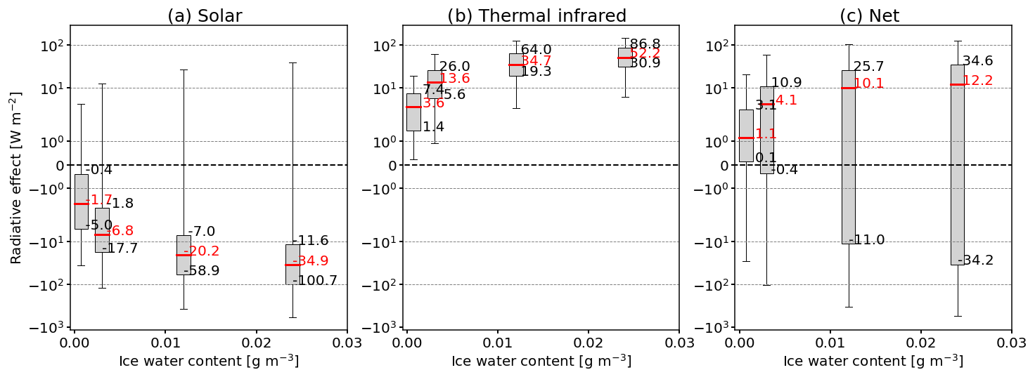
Figure 8 Same as Fig. 5 but as a function of ice water content IWC (in g m⁻³). For better legibility, only IWC values up to 0.03 g m⁻³ are plotted.

Figure 8a reveals that with increasing IWC, the median of ΔF_sol becomes more negative (intensification of the cooling effect in the solar part of the spectrum). The steepest increase is found for IWC < 0.012 g m⁻³, while for IWC ≥ 0.012 g m⁻³, the solar cloud RE saturates. At the same time, Q_ΔF,sol, given by Eq. (21), increases, indicating an enhanced sensitivity of ΔF_sol on the free parameters. The minimum and maximum values of ΔF_sol result from clouds over a highly reflective surface (α_srf = 1) and clouds containing crystals with the smallest r_eff = 5 µm.

For ΔF_tir, the increase in IWC leads to an intensified warming effect (Fig. 8b). Again, this is caused by the increase in the total particle scattering and absorption cross sections. Similar to ΔF_sol, the steepest increase in ΔF_tir appears for IWC < 0.012 g m⁻³, while for larger IWC, the medians approach an almost constant level, and a further increase in IWC has only a limited effect on ΔF_tir. The resulting ΔF_net (Fig. 8c) ranges from −543.2 to 125.5 W m⁻² and is skewed to positive ΔF_net with median values between 1.1 and 12.2 W m⁻².

Figure 9 Same as Fig. 5 but as a function of effective crystal radius r_eff (in µm).

The size of ice crystals also influences the cloud RE, with a larger sensitivity of ΔF_sol on r_eff than ΔF_tir (Baum et al., 2005b). Figure 9a illustrates that cirrus with the smallest r_eff are associated with the most intense cooling effect in the solar range, leading to ΔF_sol between −944.5 and 80.0 W m⁻². Small crystals and high number concentrations lead to higher α_cld,ice in the solar range compared to fewer and larger crystals (Stephens et al., 1990; Zhang et al., 1994). For the smallest crystals in the simulations, a median ΔF_sol of −38.6 W m⁻² is determined. For increasing r_eff, the cooling effect in the solar range decreases and tends towards ΔF_sol of −1.8 W m⁻². The intensified solar cooling (more negative ΔF_sol) with decreasing r_eff is associated with an increase in the ice crystal number concentration while keeping IWC constant, which is also known as the cloud albedo effect. In addition, ice crystals with larger r_eff are characterized by enhanced forward scattering. Hence, less radiation is scattered to the sides or backwards into space. Figure 9a shows that clouds with larger r_eff are less sensitive to the effect of the free parameters as the interquartile range decreases strongly from Q_ΔF,sol (r_eff=5 µm) = 108.7 W m⁻² to Q_ΔF,sol (r_eff=85 µm) = 8.0 W m⁻². Similarly, Fig. 9b shows the strongest TIR heating for the smallest crystals/highest N_ice. Such clouds have the largest total absorption cross section and act almost as blackbodies in the TIR (Stephens et al., 1990; Zhang et al., 1994). However, an increase in r_eff, while fixing IWC, leads to a reduction in ΔF_tir, which is caused by the lower total particle scattering and absorption cross sections. Q_ΔF,tir decreases from 58.8 W m⁻² for r_eff=5 µm to 18.5 W m⁻² for r_eff=85 µm. Median values of ΔF_net, shown in Fig. 9c, indicate only a net cooling for r_eff=5 µm, with −1 W m⁻², whereby elsewhere a net warming is dominant, with ΔF_net between 2.6 and 4.5 W m⁻². Simultaneously, Q_ΔF,net slightly decreases, which indicates the reduced impact of the remaining free parameters for large crystals. The presented dependencies, especially for small r_eff, of solar, TIR, and net ΔF on r_eff and IWC agree with previous studies, e.g., from Hansen and Travis (1974) but particularly Fu and Liou (1993) and Zhang et al. (1999).

3.4 Multi-dimensional dependencies on θ, α_srf, r_eff, and IWC

The previous analysis aimed to sample the 8D hypercube in a series of 1D cross sections to focus on the general distribution of ΔF that results from a single parameter. This likely masks the dependencies of ΔF on specific parameter combinations that are closely interconnected. Subsequently, we focus on a detailed analysis, particularly in the solar wavelength range, to highlight the dependencies among Sun geometry, surface albedo, and cloud properties – especially r_eff and IWC.

3.4.1 Solar radiative effect

Figure 10 shows ΔF_sol as a function of IWC and r_eff for combinations of α_srf (columns) and θ (rows). Moving from the left column to the right column, the surface becomes more reflective (increasing α_srf), and going from the top row to the bottom row, the Sun approaches the horizon (increasing θ).

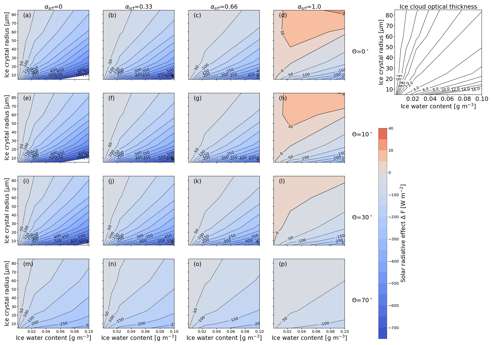
Figure 10 Solar cloud radiative effect ΔF_sol (in W m⁻²) sampled into a 2D parameter space of ice water content (IWC; in g m⁻³) and effective radius (r_eff; in µm). Each panel represents combinations of surface albedo α_srf and solar zenith angle θ. Blue values indicate negative ΔF_sol (cooling), and red values indicate positive ΔF_sol (warming). The contour lines provide a direct measure of the sensitivity to the indicated parameters. The top-right panel shows, for reference, the cloud optical depth τ at 550 nm wavelength that corresponds to the combinations of r_eff and IWC shown in the other panels.

Figure 10a represents non-reflective surfaces and the Sun at the zenith. In these cases, and focusing on ice crystals with r_eff>30 µm, the contour lines are well separated. A wide spacing of the contour lines indicates a low sensitivity of ΔF_sol on IWC and r_eff. In those regions, ΔF_sol ranges from 0 to −450 W m⁻² (cooling), with an intensification of ΔF_sol for decreasing r_eff. The contour lines become closer for r_eff<30 µm and align with the x axis, which indicates an increase in the sensitivity of ΔF_sol, particularly with respect to r_eff, as is expected from Fig. 2.

For the Sun at zenith and cirrus above reflective surfaces ($\mathrm{0}<{\mathit{\alpha }}_{\mathrm{srf}}<\mathrm{1}$), the sensitivity with respect to IWC and r_eff is generally reduced. This results from the increasing contribution of surface-reflected upward irradiance, which progressively dominates ΔF_sol of the cirrus. ΔF_sol is essentially a measure of the contrast between α_srf and α_cld,ice, with α_cld,ice mostly being dependent on r_eff and IWC. In case of a highly reflective surface (α_srf≥0.6; Fig. 10d), the predominant cooling in the solar spectrum turns into a warming effect for most of the combinations, with ΔF_sol up to 15–20 W m⁻². Only ice clouds with r_eff<20–30 µm and IWC ≈ 0.04–0.1 g m⁻³, i.e., high τ_ice>3, are more reflective than the surface. Such combinations of r_eff<20 µm and IWC ≈ 0.04–0.1 g m⁻³ are associated with ice crystal number concentrations that are rarely observed in nature, except for some cases of young contrails (see Fig. 1 in Krämer et al., 2016).

For cirrus over non-reflective or slightly reflective surfaces (α_srf≤0.33) and the Sun at an intermediate solar zenith angle (θ≥30^∘), the contour lines separate, and the sensitivity of ΔF_sol on r_eff and IWC is reduced. However, this effect is less pronounced compared than a change in α_srf. For Sun positions closest to the horizon (θ=70^∘) and above highly reflective surfaces (α_srf=1), ΔF_sol in Fig. 10p is characterized by a generally low sensitivity over the entire range of IWC and r_eff. In spite of the warming effect for α_srf=1 and θ≤30^∘, the slant optical path of the incident radiation through the cloud reduces the surface influence and leads to a cooling effect with ΔF_sol in the range of −5 to −100 W m⁻².

3.4.2 Thermal-infrared and net radiative effect

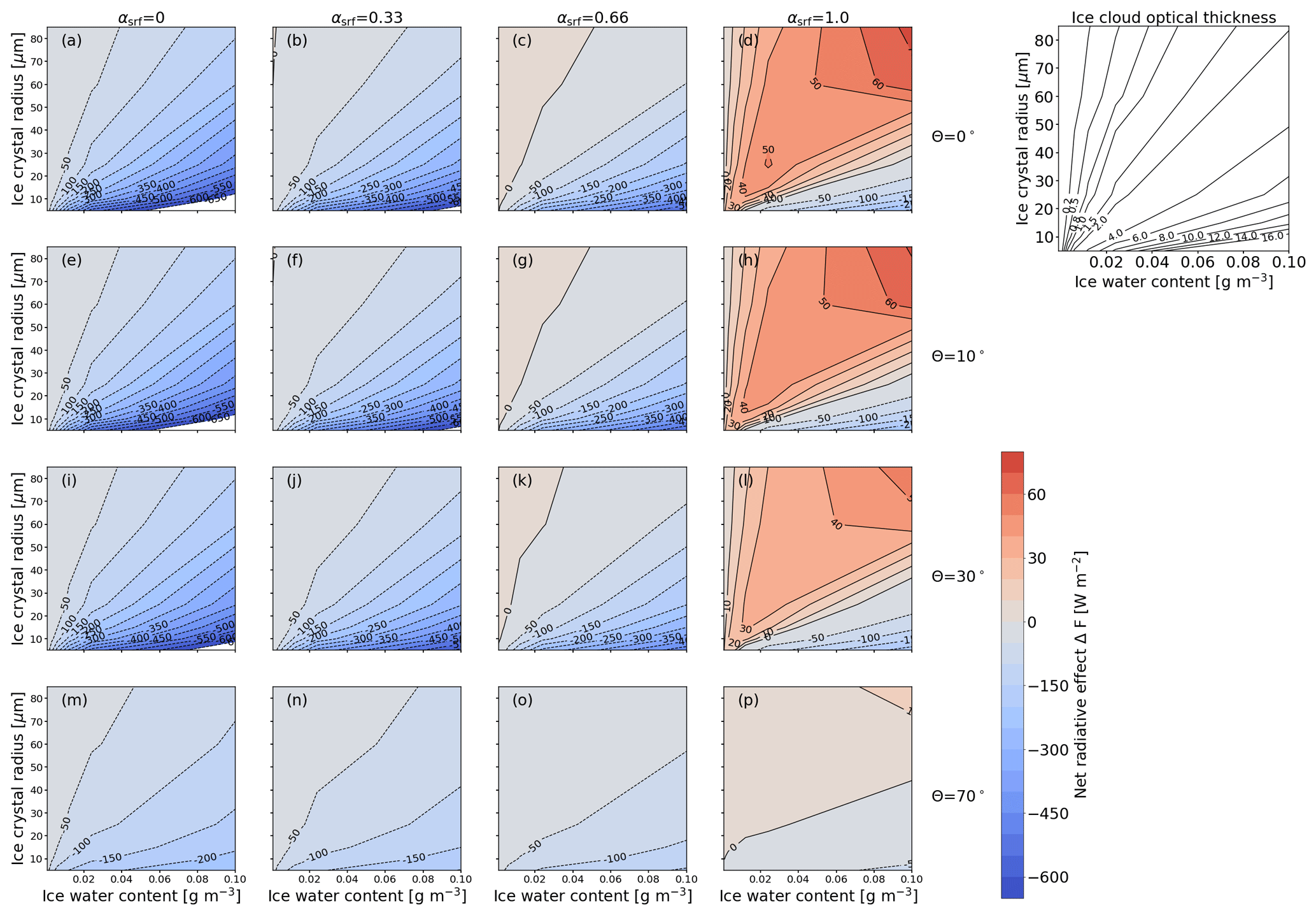
The TIR component of ΔF is insensitive to changes in θ and α_srf, and only combinations of IWC and r_eff are of relevance. In the TIR, the surface is approximated by a blackbody with a wavelength-independent emissivity equal to one. The resulting distributions of ΔF_net, shown in Fig. 11, are dominated by the contribution of ΔF_sol and, therefore, are characterized by similar sensitivities. The strongest gradient of ΔF_net on IWC and r_eff are found for θ≈0^∘ and α_srf=0 (Fig. 11a). With increasing α_srf, ΔF_net becomes positive for the majority of the combinations of IWC and r_eff (Fig. 11d), with the net warming being most pronounced for α_srf=1 (Fig. 11d). It is further noted that for α_srf=1, θ≤30^∘, and τ_liq<1, ΔF_net is positive and almost exclusively sensitive to IWC, while for α_srf=1, θ≤30^∘, and τ_liq>1, ΔF_net also becomes sensitive to r_eff. In addition, regions that have a net cooling effect, i.e., at high N_ice values, are exclusively sensitive to r_eff. The cloud can have a net cooling effect when the Sun is close to the horizon (Fig. 11p), with almost no sensitivity to r_eff and IWC.

Figure 11 Same as Fig. 10 but for ΔF_net (in W m⁻²).

3.5 Sensitivity of atmospheric profile, surface temperature, relative humidity, ice cloud altitude, and ice cloud geometric thickness

Within this study, the atmospheric profiles, the surface temperatures T_srf, and the vertical location of the ice cloud are coupled. For example, the selection of the US standard atmosphere is directly linked to a surface temperature of T_srf = 288.2 K. T_srf is equal to the lowermost temperature value in the respective AP. The vertical position of the ice cloud depends on the temperature of the AP and the selected cloud-top temperature T_cld,ice (see Appendix B and Fig. B1a–b therein).

Figure 12 Same as Fig. 5 but for surface temperature T_srf (in K).

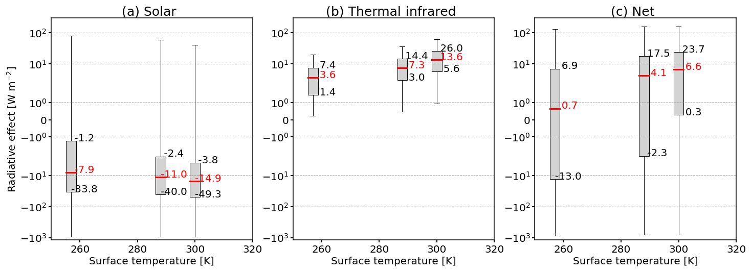
Figure 12a shows that variations in T_srf have an effect on ΔF_sol, with the differences in the median ΔF_sol of up to ±7 W m⁻². Generally, larger effects are found for the TIR component, where an increase in T_srf enhances the temperature difference between surface and cirrus, which leads to an intensification of the TIR heating (see Eq. 19 and Corti and Peter, 2009), thus shifting the median ΔF_tir from 3.6 to 13.6 W m⁻² (Fig. 12b). Simultaneously, the distributions broaden with increasing T_srf, with Q_ΔF,tir ranging from 1.4 to 7.4 W m⁻² (257.2 K) and 5.6 to 26.0 W m⁻² (299.7 K), which results from the warmer and moister tropical profile compared to the drier sub-Arctic profile. As a result of the almost constant ΔF_sol and the increase in ΔF_tir, the net heating effect is enhanced with medians ranging between 0.7 and 6.6 W m⁻².

Figure 13 Same as Fig. 5 but for ice cloud temperature T_cld,ice (in K).

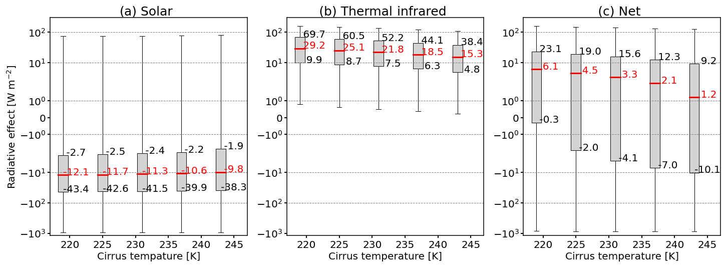
The effect of variations in T_cld,ice is shown in Fig. 13a–c. Increasing T_cld,ice reduces the temperature difference between surface and ice cloud and therefore the TIR heating effect (Fig. 13b). Median ΔF_tir values are reduced from 29.2 to 15.3 W m⁻² when T_cld,ice is increased from 219 to 243 K. Compared to the impact of T_srf, which was varied over a range of 42.5 K, shifting the cloud in the vertical has only a minor effect on ΔF_tir and ΔF_net, as the variation in T_cld,ice spanned only 24 K. The resulting net effect from variations in T_cld,ice leads to medians between 1.2 and 6.1 W m⁻² for T_cld,ice of 219 and 243 K, respectively.

The previously mentioned impact of T_srf on ΔF_sol is traced back to (a) the different optical path length through the atmosphere because of variations in cloud-top altitude and (b) the different water vapor concentration due to the three applied APs. The effect of varying RH profiles was investigated by manipulating the original RH profiles by ±20 % to represent the variability in RH reported by Anderson et al. (1986). The RT simulations were performed for a sub-set of the parameter space with fixed T_cld,ice = 231 K, α_srf = 0, and τ_liq = 0. The effects on solar, TIR, and net ΔF are quantified by their absolute and relative differences. Variations in RH have only a small effect on ΔF_sol, with maximal ±0.15 W m⁻² (±0.4 %) among all profiles. A slightly larger impact is found for ΔF_tir, with up to ±1.45 W m⁻² (±4.1 %) in case of the warm and moist tropical profile (afglt). Less affected are the standard atmosphere (afglus), where ΔF_tir varies by ±0.9 W m⁻² (±3.2 %), and the dry sub-Arctic profile (afglsw), with variations in ΔF_tir of ±0.3 W m⁻² (±2.4 %). Consequently, afglt has the largest variation in ΔF_net of ±0.8 W m⁻² (±8 %) and is followed by ±0.6 W m⁻² (±3.8 %) for afglus and ±0.2 W m⁻² (±0.6 %) for afglsw. Scaling the original RH profiles showed that variations in the RH profile explicitly influence the TIR wavelength range but particularly the net RE. This analysis suggests that the variations in RH have to be considered to be a potential source of variability when using this publicly available data set.

All simulations within this study were performed for a fixed cloud geometric thickness dz of 1000 m. In reality, however, dz is likely to vary over the cirrus lifetime, for example, due to the sedimentation of ice crystals or vertical winds. The effect of changing dz is quantified by a dedicated sensitivity analysis of ΔF for a sub-sample of the full parameter range (Table 4). A similar sub-parameter space is used as was done for the RH sensitivity but additionally fixing T_srf = 288 K, i.e., using the afglus profile. With τ_ice being proportional to the IWP of the cloud (Eq. 10), the IWP of the 1000 m reference and solar τ_ice are kept constant, and the IWC for the clouds with dz of 500 and 1500 m clouds is scaled accordingly.

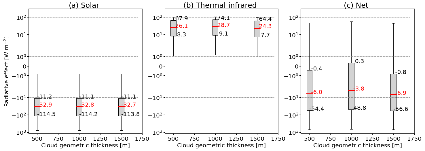
Figure 14 Same as Fig. 5 but for the cloud geometrical thickness dz (in m) and only for a sub-sample of the parameter space. Values for ice cloud temperature T_ice = 231 K, surface temperature T_srf = 288.2 K, surface albedo α_srf=0.15, and liquid water cloud optical thickness τ_liq = 0 are given. Values for solar zenith angle θ, ice water content IWC, and effective radius r_eff are varied.

As expected from Eq. 10, the resulting effect on median ΔF_sol, given in Fig. 14, is almost negligible, with ±0.1 W m⁻² (±0.3 %). Differences in the median ΔF_tir are up to ±0.6 W m⁻² (±3.5 %), which leads to differences in the median ΔF_net of ±0.6 W m⁻² (±6.2 %). The relevant relative differences in ΔF_tir and ΔF_net are explained by the varying cloud base altitude, which modifies the vertical distribution of IWC and the temperature of the cloud base, which determines the amount of emitted radiation. In addition, geometrically thin clouds with low τ_ice act as graybodies, while with an increase in dz, cirrus clouds become opaque and act as more efficient blackbodies (Corti and Peter, 2009). Fu and Liou (1993) further reported that cirrus with small r_eff reflect solar radiation at the cloud top (solar cooling) but absorb TIR radiation at the cloud base (TIR warming), which creates a temperature gradient within the cloud that depends on dz. From the dz sensitivity analysis, it is found that dz can be neglected in the solar wavelength range but is of relevance for ΔF_tir and especially ΔF_net, where the absolute values are small. This partly agrees with the findings from Meerkötter et al. (1999), who showed that solar, TIR, and net ΔF are only slightly sensitive to changes in dz with solar, TIR, and net ΔF below 2 W m⁻² under the premise of a constant ice water path (IWP). The presented simulations indicate ΔΔF_sol of 2 W m⁻², which is comparable to Meerkötter et al. (1999), but we found slightly higher ΔΔF_tir and ΔΔF_net of 4.5 and 3.1 W m⁻², respectively.

3.6 Sensitivity on underlying liquid water cloud

The impact of an additional liquid water cloud on the cirrus ΔF is presented in Fig. 15. A liquid water cloud optical thickness τ_liq=0 is equivalent to the absence of secondary clouds, and such conditions lead to the strongest ΔF_sol, with a median of −16.1 W m⁻². By gradually increasing τ_liq, the reflected upward irradiance overlays and masks the impact of the surface. In general, the response of ΔF_sol on τ_liq is comparable to that of an increase in α_srf. Introducing a cloud with τ_liq=5 slightly enhances the cooling in the solar spectrum ΔF_sol from −11.5 to −7.6 W m⁻². More notable is the reduction of the variability in ΔF_sol, with the distribution becoming narrower and reducing Q_ΔF,sol from 54.8 to 23.8 W m⁻².

Figure 15 Same as Fig. 5 but for the underlying liquid water cloud optical thickness τ_liq.

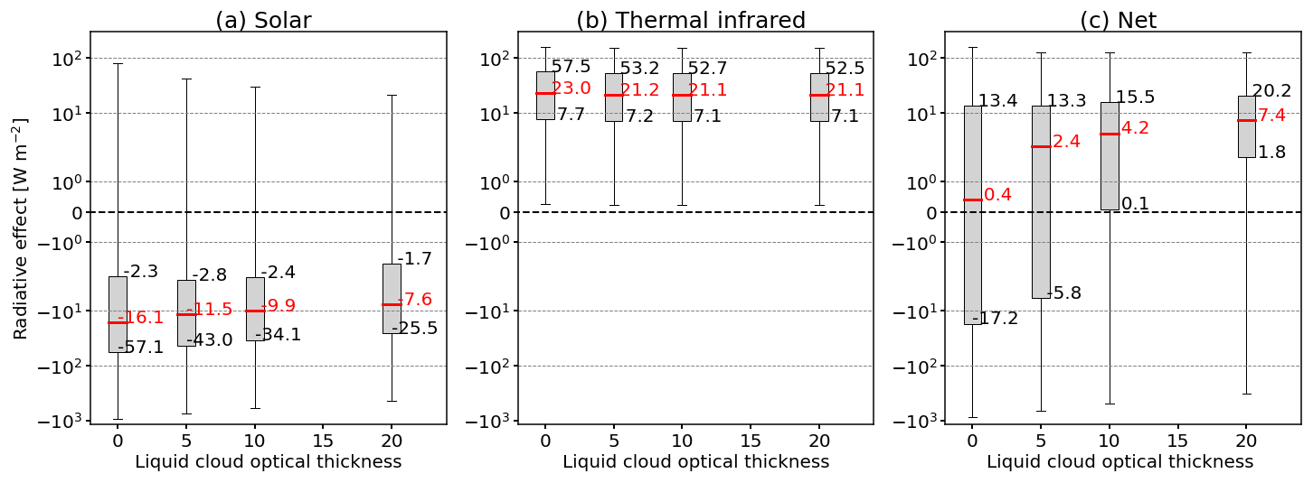
An increase in τ_liq from 0 to 5 shifts the median ΔF_tir from 21.1 to 23.0 W m⁻². With a further increase in τ_liq, the medians remain almost constant, while the Q_ΔF,tir slightly decreases. The reduction in the maximum ΔF_tir is a consequence of the attenuated temperature difference ΔT between the liquid water cloud and the ice cloud compared to the surface. The effect on ΔF_tir is small, as the change in temperature from surface to liquid water cloud is small in the case of the US standard atmosphere, where ΔT=5 K.

As a result of the reduced cooling in the solar spectrum and the stronger warming in the TIR spectrum, the net heating of the ice clouds intensifies with increasing τ_liq. The median ΔF_net is shifted from 0.4 to 7.4 W m⁻², with an accompanying decrease in the overall variance. While for τ_liq<5, slightly fewer than 50 % of the combinations exert a potential net cooling by the cirrus, positive ΔF_net is dominating for larger τ_liq.

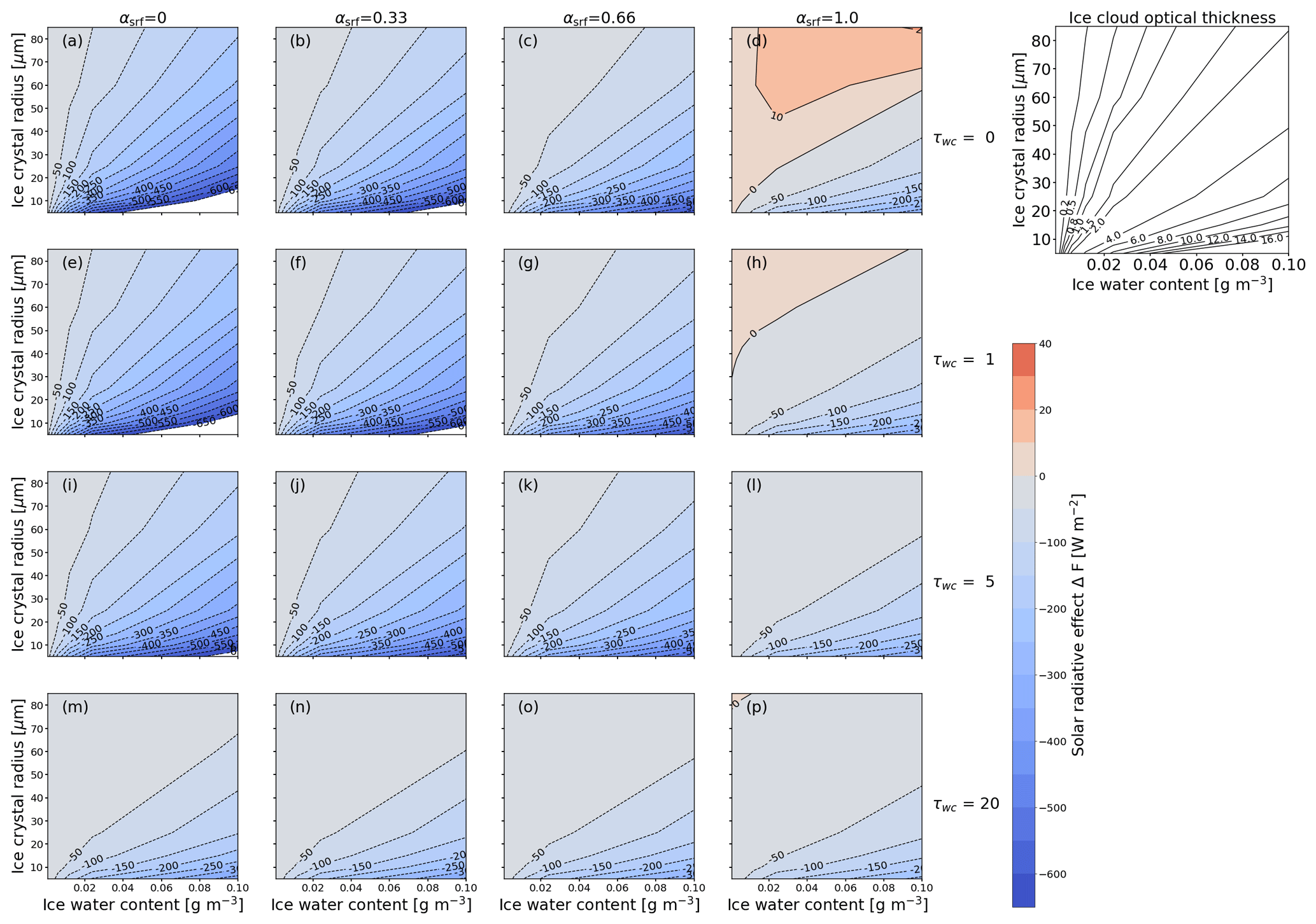
Figure 16 Same as Fig. 10 but ΔF_sol (in W m⁻²) and combinations of surface albedo α_srf and cloud optical thickness τ_liq of the underlying liquid water cloud.

Figure 16 shows ΔF_sol, depending on IWC and r_eff, separated for α_srf (columns) and τ_liq (rows). In the presented cases, a θ of 10^∘ is selected as the influence of the surface, and an additional cloud layer is of higher importance when the Sun is close to the zenith. Due to the selection of θ, the top row in Fig. 16 is the same as the second row in Fig. 10, with similar characteristic features in the distribution and sensitivity; the largest RE appears over dark surfaces (α_srf=0) in combination with clouds containing the largest ice number concentrations N_ice due to small r_eff and larger IWC. Increasing r_eff and/or reducing the IWC weakens ΔF_sol. Introducing the second cloud layer and gradually increasing τ_liq generally reduces the sensitivity of the ice cloud microphysical properties and the ice cloud RE. For the special case of α_srf=1, the introduction of a liquid water cloud turns the previous solar warming (ΔF_sol ≈ 10 W m⁻²) into a solar cooling effect of up to ΔF_sol = −15 W m⁻² for typical τ_ice of contrails.

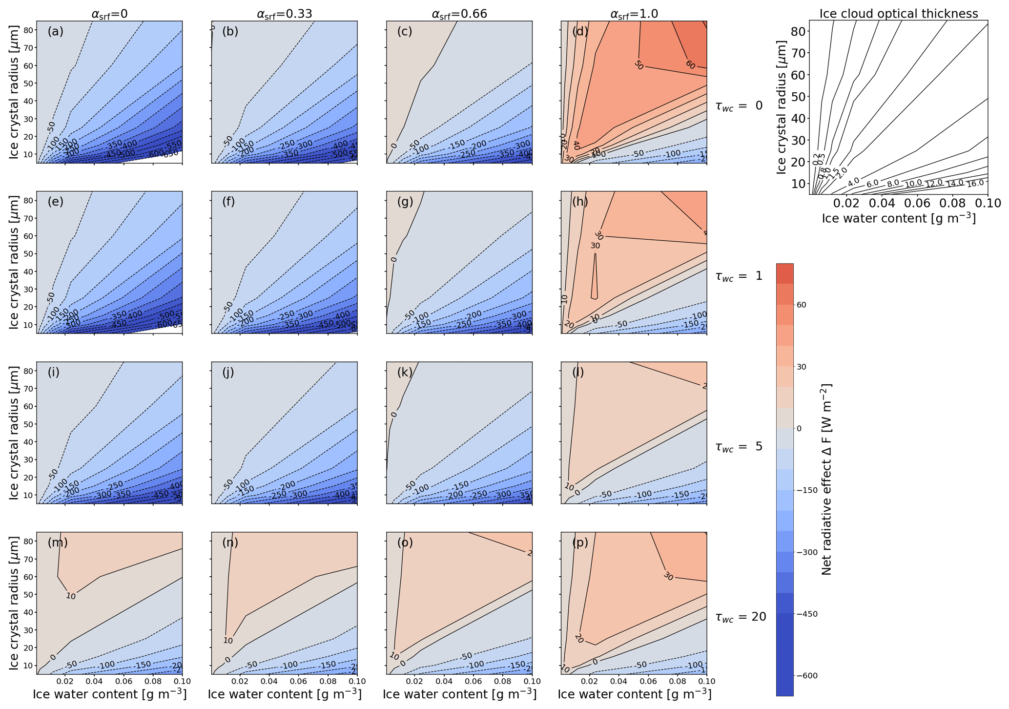
Figure 17 Same as Fig. 11 but for ΔF_net (in W m⁻²) and combinations of surface albedo α_srf and cloud optical thickness τ_liq of the underlying liquid water cloud.

As shown in Fig. 15, the second cloud layer at z=1500 m modifies ΔF_tir only slightly, and multi-dimensional dependencies with respect to IWC, r_eff, α_srf, and τ_liq are weak, leading to homogeneous distributions (not shown here). Figure 17 illustrates the variations in ΔF_net. For combinations of α_srf≤0.66 and τ_ice≤5, ΔF_net is determined by the solar component and its sensitivities. Special attention should be given to conditions with α_srf≥0.66 and τ_ice>0.8, where ΔF_net turns from a cooling into a warming effect. This is due to the reduced ΔF_sol and the domination by ΔF_tir. In these situations, ΔF_net ranges between 0 and 60 W m⁻². Increasing τ_liq leads to a reduction in the sensitivity of ΔF_net with respect to the r_eff and IWC of the ice cloud. An exception is clouds with extreme N_ice, where an increased cooling effect in relation to r_eff occurs. Furthermore, cirrus over optically thick underlying clouds (last row) has a predominantly net warming effect.

4 Discussion

This study focused on the cloud RE of homogeneous, horizontally infinite ice cloud layers and neglected horizontal photon transport. The vertical and horizontal structure of ice clouds, i.e., distribution of ice water content, is typically heterogeneous, which is one reason for differences and uncertainties between the 1D-simulated and the actual RE of such clouds (Fauchez et al., 2017, 2018). Additional differences originate from the independent pixel approximation (Cahalan et al., 1994).

For completeness and to raise awareness of potential uncertainties in the present simulations due to the effects of cloud heterogeneity and 3D scattering on the estimated RE, we provide a brief overview of the relevant literature. The majority of past cirrus and contrail studies that quantified the RE sensitivity were based on 1D RT simulations (Strauss et al., 1997; Meerkötter et al., 1999; Fahey et al., 1999; Stuber et al., 2006). While aged and spread contrails might be approximated as thin plane-parallel layers within a homogeneous atmosphere (Minnis et al., 1999), younger contrails and cirrus are heterogeneous in their horizontal and vertical distribution of IWC. The first study that investigated 3D radiative effects was performed by Schulz (1998). This study was followed by Gounou and Hogan (2007) and Forster et al. (2012), who used 3D Monte Carlo simulations and found differences in contrail solar RE between 1D and 3D simulations ranging from 5 to 40 %. The largest deviations were found for extreme cases, e.g., large solar zenith angle (Sun close to the horizon). With the Sun illuminating the contrail or cirrus from the side, extinction and absorption within the cloud increases, and the scattering at cloud sides becomes more important compared to an illumination from above. Enhanced scattering at cloud sides also increases the likelihood that photons become scattered back into space instead of being absorbed. Such effects are not captured by 1D RT simulations. Concerning the TIR wavelength range, Gounou and Hogan (2007) found that horizontal photons transport can increase contrail radiative effect by around 10 %, which has to be considered in the calculation of the contrail net radiative effect.

However, there is no systematic bias in solar, TIR, and net RE between 1D and 3D simulations, and the deviations decrease with increasing cloud homogeneity. More specifically, the differences between 1D and 3D simulations change in magnitude and sign, depending on the cloud heterogeneity and the solar illumination geometry. We employ 1D simulations as the total number of simulations performed within this study, and the computational cost for full 3D RT simulation is unpractical. Therefore, we highlight that the provided data set can be used for situations that can be approximated by plane-parallel clouds and solar zenith angles smaller than 70^∘. Results should be used carefully by considering that 3D radiative effects introduce uncertainties.

The eight selected parameters discussed in this study were found to be the most influential on the cirrus RE. The selection is further supported by earlier studies, e.g., Fu and Liou (1993), Zhang et al. (1999), Meerkötter et al. (1999), Yang et al. (2010), or Mitchell et al. (2011). However, not all potential factors that impact the cirrus RE can be considered in such a parametric study. Additional influences like aerosol layers, more complex surface albedo, or multiple overlapping cirrus clouds and contrails have not been investigated here and represent additional degrees of freedom. For example, previous studies found that aerosols have only a minor influence on contrail RE (Meerkötter et al., 1999), and Sanz-Morère et al. (2021) reported that the impact of overlap between contrails on their RE is negligible.

5 Summary

The net radiative effect ΔF (RE) of cirrus and contrails depends on multiple factors related to the microphysical and macrophysical cloud properties, the cloud optical properties, and radiative properties of the environment. The presented study aimed to separate the effect of the following eight selected parameters on the cirrus RE: solar zenith angle θ, ice water content IWC, ice crystal effective radius r_eff, cirrus temperature T_cld,ice, surface albedo α_srf, surface temperature T_srf, liquid water cloud optical thickness τ_liq of an underlying cloud, and three ice crystal shapes. In total, 283 500 radiative transfer (RT) simulations have been performed with the libRadtran RT code by varying the eight parameters within the ranges that are typically associated with natural cirrus and contrails. The RT simulations were performed with a 1D solver (plane-parallel clouds) and 3D scattering effects were not considered, despite the fact they are known to become relevant for large solar zenith angles (θ>70^∘). Specific cases or sub-samples were selected and discussed, while the entire set of results is made available as a NetCDF file (Wolf et al., 2023).

For the presented cases, the cirrus RE was discussed separately for not only the solar ΔF_sol and thermal-infrared (TIR) ΔF_tir part of the spectrum but also for the combined net RE. Comparing to a chosen reference with θ=0^∘, $T_{\mathrm{cld},\mathrm{ice}}=\mathrm{219}$ K, α_srf=0, T_srf=299.7 K, IWC = 0.024 g m⁻³, r_eff = 85 µm, τ_liq = 0 (no liquid water cloud), and the resulting τ_ice=0.46 (at 550 nm), it was found that r_eff has the largest impact on solar, TIR, and net RE. The second most important parameter is the IWC, which impacts ΔF_sol and ΔF_tir equally. In the selected case, ΔF_sol and ΔF_tir have opposite signs, meaning that the IWC has a relatively small impact on ΔF_net. It has to be noted that the counterbalancing effect only appears during daytime, when ΔF_sol≠0 W m⁻². Whether r_eff or IWC is the most impactful parameter depends on the r_eff chosen as a reference. However, the dominance of r_eff and IWC over all other parameters remains. At night, ΔF_net equals ΔF_tir, and the cirrus heats the Earth–atmosphere system. After r_eff and IWC, the solar RE of cirrus is determined by θ, α_srf, τ_liq, and the ice crystal shape, in descending priority. The RE in the TIR spectrum is dominated by T_srf, T_cld,ice, τ_liq, and the ice crystal shape. The combined net RE is controlled by α_srf, θ, and T_srf, which are sorted in decreasing importance. The relevance of selected parameters can differ for other τ_ice and ambient conditions.

The impact of individual parameters on the solar, TIR, and net RE was further investigated and quantified by sub-sampling the entire set of simulations by fixing one parameter at a time, while the remaining parameters were allowed to vary. This can be interpreted as a type of a sub-sampling, by averaging all unfixed values of RE, to project ΔF onto the 1D space.

• Variations in θ have no influence on ΔF_tir but only on ΔF_sol. The majority of simulated ΔF_sol becomes more intense (stronger cooling) with increasing θ and reaches a maximum for θ between 50–70^∘. For further increasing θ, the cooling effect in the solar wavelength range declines. The exact location of the maximum ΔF_sol is primarily dependent on α_srf. Increasing θ, the impact of the other free parameters and the resulting ΔF_sol is reduced. Consequently, the majority of the simulations with negative ΔF_sol are exceeded by positive ΔF_tir, which leads to a positive median ΔF_net (warming).

• The projection of ΔF_net for varying α_srf showed that cirrus primarily cools in the solar wavelength range, except for highly reflective surfaces with α_srf approaching 1, e.g., over ice-covered regions. Contrarily, ΔF_tir is mostly positive and unaffected by the variations in α_srf. ΔF_tir determines the resulting ΔF_net, which leads to a net heating effect when α_srf exceeds the critical range of 0.25–0.3.

• An increase in IWC intensifies the cooling in the solar and the heating in the TIR. As both effects compete against each other and ΔF_tir dominates ΔF_sol, the resulting net RE is a warming. An exception appears for the largest IWC, where the median ΔF_net is negative. Simultaneously, the increase in IWC causes an enhanced impact of the free parameters and associated uncertainties.

• Clouds with similar IWC but larger r_eff are comprised of fewer ice crystals, which reduces the cloud reflectivity (cloud albedo effect). Over the entire range of r_eff the sub-sampled data set is characterized by a negative ΔF_sol that is most intense for the smallest crystals. Similarly, ΔF_tir is largest for small crystals and decreases for large crystals. While the solar and TIR ΔF become less intense with r_eff, the decrease is more pronounced for ΔF_sol, such that cirrus primarily has a positive ΔF_net. An exception is clouds with the smallest r_eff and high IWC that occur only in contrails that just formed over non-reflective surfaces.

• The surface temperature T_srf and ice cloud temperature T_cld,ice only affect the TIR component of ΔF. Increasing the absolute difference between T_srf and T_cld,ice leads to an intensified TIR and resulting net heating effect.

• An underlying liquid water cloud with an increasing τ_liq leads to a reduction in solar ΔF_sol. Simultaneously, the TIR heating remains almost constant, reducing the negative ΔF_net (cooling) that is finally turned into positive ΔF_net (net warming) for the majority of simulated cases.

Appendix A: Overview over the multi-parameter dependencies

Figures A1 and A2 show solar ΔF_sol and TIR ΔF_tir (upper diagonal) and net ΔF_net (lower diagonal) for combinations of parameters indicated along the x and y axes. Both plots are intended to provide an overview over the multi-parameter dependencies. Within each sub-panel, ΔF is given as a function of the x and y axes, while the other parameters are set to constant values that are representative of contrails and cirrus clouds. For example, the “IWC–SZA” panel shows ΔF as a function of IWC, with θ=30^∘, T_cld,ice = 231 K, r_eff=25 µm, α=0.15, T_srf=288 K and without a second liquid water cloud (τ_liq=0). This can be understood as a 2D cross section of the 8D hypercube. The black arrows indicate the gradient of the field. The gradient is computed with second-order central differences and one side difference at the boundaries of the field. The length of the arrow is only representative of an individual field and cannot be compared with the other fields, as it depends on the units of the parameters. Therefore, the arrows are normalized and can only be interpreted for their direction and not for their length.

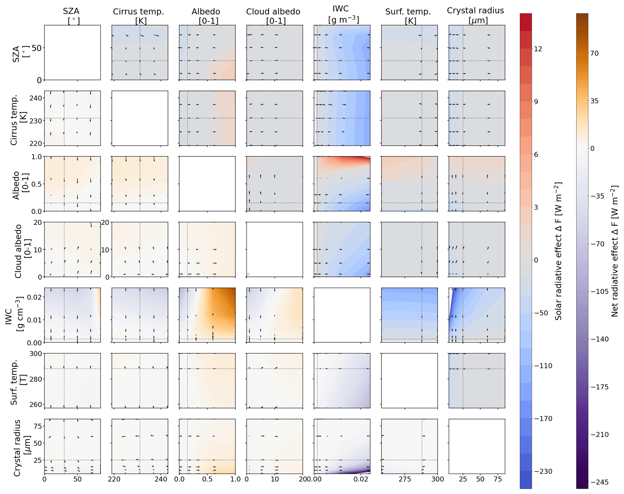
Figure A1 The upper diagonal panels show the plot of median solar ΔF_sol projected in a 2D parameter space. Blue colors indicate negative ΔF_sol (cooling), while red colors indicate positive ΔF_sol (warming). The lower diagonal panels show the same as the upper diagonal panels but for median net ΔF_net. Purple shades indicate negative ΔF_net (cooling), while orange shades indicate positive ΔF_net (warming). All ΔF have the same units (given in W m⁻²). The black arrows point to the direction of the steepest slope.

Figure A2 Same as Fig. A1 but the upper diagonal panels present median ΔF_tir. All ΔF have the same units (given in W m⁻²).

Appendix B: Atmospheric profiles of temperature and relative humidity

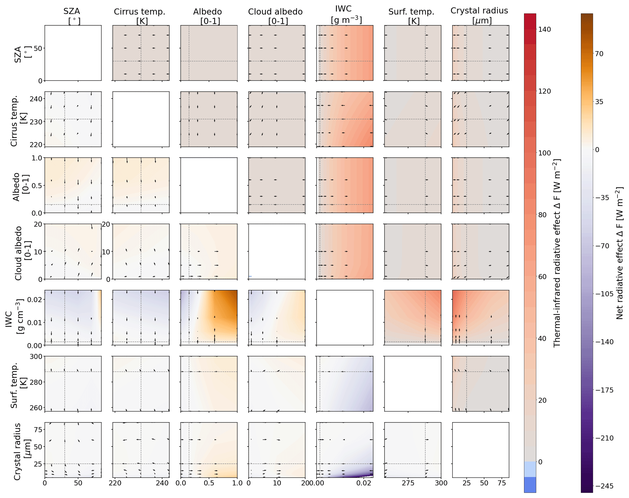
The radiative transfer simulations within the present study use the atmospheric profiles from Anderson et al. (1986) that are provided in the libRadtran package. To cover a wide range of temperature conditions, three atmospheric profiles were selected, which represent the sub-Arctic, mid-latitude, and tropical conditions given by the afglsw, afglus, and afglt profiles, respectively. The vertical temperature profiles range from 0 to 120 km and are visualized in Fig. B1a. Figure B1b presents a close-up view, and Fig. B1c shows the relative humidity profile for 0 to 20 km. The position of the low-level liquid water cloud between 1000 and 1500 m is indicated by the gray shaded area. The positions of the ice cloud altitude are indicated by the colored dots.

According to Anderson et al. (1986), the presented profiles are subject to variations between 10 % and 30 %. Therefore, we multiplied the original profiles by factors of 0.8 and 1.2 to (i) partly account for this variation and (ii) to estimate the influence of variations in RH on the simulated solar, TIR, and net RE. The modified profiles with ±20 % are indicated by pale colors in Fig. B1c.

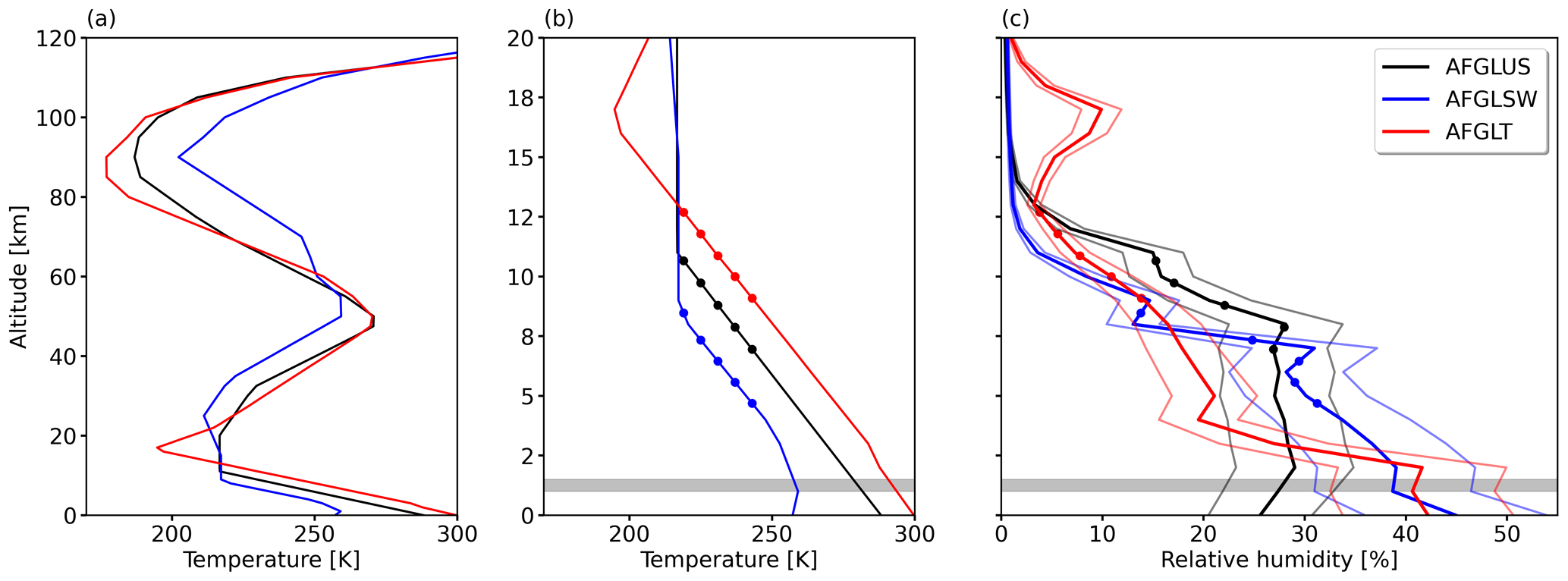
Figure B1 Profiles of temperature (a, b) and relative humidity (c) used for the radiative transfer simulations. The sub-Arctic (afglsw), mid-latitude (afglus), and tropical (afglt) profiles are given in blue, black, and red, respectively. The modified profiles with ±20 % are indicated by pale colors. The positions of the simulated ice water cloud are indicated by the colored dots for each profile. The position of the low-level liquid water cloud is indicated by the gray shaded area.

Appendix C: Simulation time and accuracy

The radiative transfer solver DISORT (Stamnes et al., 1988; Buras et al., 2011) allows us to select 2 N numbers of streams to be used in the radiative transfer simulations. The higher number of streams increases not only the accuracy of the simulations but also the computational time. To obtain sufficient accuracy while keeping the computational time reasonable, the optimal trade-off was estimated by progressively increasing the number of streams from 4 to 48. The simulation with 48 streams is regarded here as the reference with the highest accuracy and computational time.

The number of streams and the timing of the RT simulations are estimated on the basis of a specific parameter combination, which represents a complex cloud scene that is characterized by cloud–cloud surface interactions. The simulations are run for a solar zenith angle θ=70^∘, a cirrus temperature T_cld,ice of 233 K, a surface albedo α_srf=1, an ice water content IWC = 0.0024 g m⁻³, a surface temperature T_srf=288 K, an ice crystal effective radius r_eff=5 µm, and an additionally underlying liquid water cloud (cloud optical thickness τ_liq = 10).

The computational time that is required for the simulations depends on the available hardware. Therefore, we provide the fraction of the computational time required for n streams to a simulation with 48 streams. The accuracy is given as the relative difference between the cloud RE for a given number of streams with respect to the reference simulation.

Figure C1 shows that the relative difference in the RE decreases with an increasing number of streams (higher accuracy). A significant gain in accuracy is achieved by switching from 4 to 10 streams. For simulations with 12 to 16 streams, the relative difference remains constant at around 0.1 %. Further increasing to 24 streams provides only a slight gain in accuracy, whereas the computational time increases disproportionally. Therefore, the optimal trade-off between accuracy and computational time is obtained with 16 streams, which is the configuration used in this study.

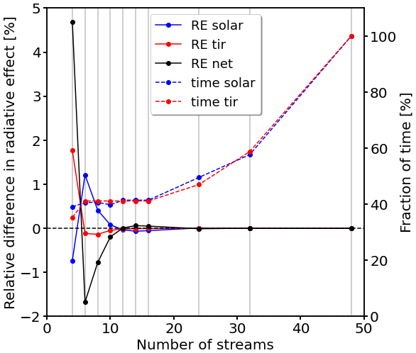
Figure C1 Relative deviation (in %) of solar (solid blue), TIR (solid red), and net (solid black) cloud radiative effect from the reference simulation calculated with 48 streams. The computational time is given as a fraction of the computational time needed for the solar (dashed blue) or TIR (dashed red) simulations using the maximum number of 48 streams.

We estimated the uncertainty that is associated with the REPTRAN “coarse” parameterization instead of the “fine” resolution by simulating one particular cloud case and running the simulation with both options. The selected simulation is characterized by a solar zenith angle θ=70^∘ for a long and slanted path through the atmosphere to maximize the impact of molecular absorption; a cirrus temperature T_cld,ice of 233 K as the center of the parameter space; a surface albedo α_srf=0.15 for moderate surface reflection; an ice water content IWC = 0.012 g m⁻³; a surface temperature T_srf=300 K to select the tropical atmospheric profile with the highest water vapor concentration; and an ice crystal effective radius r_eff=25 µm. Based on the two simulations, relative differences in the solar, TIR, and net radiative forcing ΔF of 0.4 %, 0.2 %, and 1.9 % were determined, respectively.

Appendix D: Single-scattering phase function 𝒫

The shape effect is primarily caused by differences in the extinction of radiation and the asymmetry parameter. The asymmetry parameter is a measure of the asymmetry of the phase function 𝒫 between forward and backward scattering (Macke et al., 1998; Fu, 2007). 𝒫 provides the angular distribution of the scattered direction in relation to the incident light.

As an example, Fig. D1a–d show 𝒫 at 550 nm wavelength for columns, plates, droxtals, and the Yang et al. (2013) “8–column_aggregates”, which are ice crystals consisting of eight merged columns. The phase functions are extracted from the post-processed libRadtran data set that is based on the ice optics computations from Yang et al. (2013).

All ice crystal shapes are characterized by a dominating peak in the forward direction, which drops by a factor of 10⁴ sr⁻¹ when the scattering angle Θ increases from 0 to 10^∘. For $\mathrm{10}{}^{\circ }<\mathrm{\Theta }<\mathrm{160}$^∘, 𝒫 varies between 10⁻¹ and 10¹ sr⁻¹. Towards Θ>160^∘, the phase function increases, showing enhanced backward scattering, except for the complex-shaped crystals (Fig. D1d). Further characteristics of 𝒫 are local maxima at 22^∘ scattering angles that cause halo phenomena. Additionally, non-spherical crystals (Fig. D1a, b, d) have enhanced sideward scattering compared to ice crystals with a roughly spherical shape like droxtals (Fig. D1c) or water droplets. Another characteristic is the shift in the 𝒫 from variations in the crystal radius r_eff, which is most prominent for plates and lowest for columns.

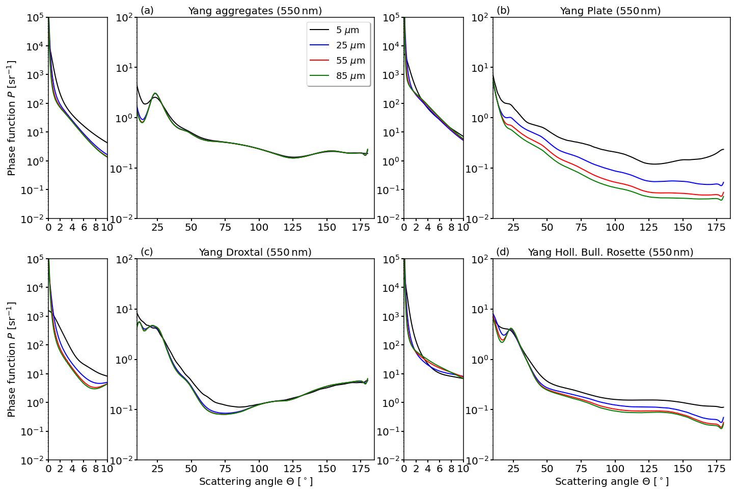
Figure D1 Phase function of four different ice crystal shapes with moderate surface roughness and four particle size distributions at 550 nm wavelength. Aggregates are represented by moderately rough aggregates of eight-element columns. Please note the two different y scales that are used to account for the different magnitudes in the forward-scattering peak. Plotted 𝒫 are post-processed phase functions from Emde et al. (2016) that are based on Yang et al. (2013). The phase functions from Emde et al. (2016) assume a crystal size distribution that follows a gamma function.