the Creative Commons Attribution 4.0 License.
the Creative Commons Attribution 4.0 License.
 | 09 Nov 2023
Analysis of insoluble particles in hailstones in China
Haifan Zhang
Xiangyu Lin
Kai Bi
Chan-Pang Ng
Yangze Ren
Huiwen Xue
Li Chen
Zhuolin Chang
Insoluble particles influence weather and climate by means of heterogeneous freezing process. Current weather and climate models face considerable uncertainties in freezing-process simulation due to limited information regarding species and number concentrations of heterogeneous ice-nucleating particles, particularly insoluble particles. Here, for the first time, the size distribution and species of insoluble particles are analyzed in 30 shells of 12 hailstones collected from China using scanning electron microscopy and energy-dispersive X-ray spectrometry. A total of 289 461 insoluble particles were detected and divided into three species – organics, dust, and bioprotein – utilizing machine learning methods. The size distribution of the insoluble particles of each species varies greatly among the different hailstones but little in their shells. Further, a classic size distribution of organics and dust followed logarithmic normal distributions, which could potentially be adapted in future weather and climate models despite the existence of uncertainties. Our findings highlight the need for atmospheric chemistry to be considered in the simulation of ice-freezing processes.
- Article
(6450 KB) - Full-text XML
- BibTeX
- EndNote


Insoluble particles, acting as the main heterogeneous ice-nucleating particles in the atmosphere (Lamb and Verlinde, 2011), influence precipitation formation and radiative forcing (Hoose and Möhler, 2012; DeMott et al., 2015) and further impact weather and climate (Vergara-Temprado et al., 2018). Temperature and vapor supersaturation are used to calculate the number concentration of ice crystal particles in microphysics parameterization rather than considering the physical properties of ice-nucleating particles in weather and climate models (DeMott et al., 2010). Few models use the freezing parameterization, which establishes a direct connection between the number concentration of ice-nucleating particles and the number concentration of ice crystals. The absence of description regarding the number concentration of ice-nucleating particles in models can result in an incorrect estimation of ice crystals and lead to significant bias in radiative simulations (Vergara-Temprado et al., 2018).
An improved description of the number concentrations of ice-nucleating particles is needed (DeMott et al., 2010) but is obstructed by a lack of complete microphysical observations of ice-nucleating particles in clouds. There are two ways to sample ice-nucleating particles: the first involves an airborne instrument, named a continuous-flow thermal-gradient diffusion chamber (Rogers et al., 2001; Prenni et al., 2009; DeMott et al., 2010); the second is done in the laboratory, where scientists conduct freezing experiments (Hoose and Möhler, 2012). In most cases, it is necessary for an aircraft to collect air parcels for measurement of the physical properties of ice-nucleating particles in the air. However, former field projects sampled air parcels in anvils of convective clouds, cirrus clouds, and winter mixed-phase stratiform clouds. No flight report or article has reported that they sampled air parcels through cores in deep convection. This phenomenon is consistent with considerations for flight security. Thus, current observations are insufficient for describing the whole convective cloud, especially the deep convection in severe storms. The absence of microphysical observations of ice-nucleating particles within severe storms leads to uncertainty in understanding cold cloud processes.
Hailstones, as a product of deep-convective clouds, serve as carriers of information within these clouds. Recently, analyses revealed large diversity in terms of the number concentration of soluble ions among hailstones from different hailstorms (Li et al., 2018). Further, the detection of soluble ions along with isotopic analysis of a huge hailstone revealed an up-and-down hailstone growth trajectory, which demonstrated that the different shells were formed at different heights (Li et al., 2020). These studies have proved that aerosol information in convective clouds may be recorded in soluble particles within hailstones (Li et al., 2018, 2020). Similarly, insoluble particles in hailstones can also record aerosol information in severe storms.
Former studies showed that species and number concentration of insoluble particles in hailstones (Vali, 1968; Rosinski, 1966; Michaud et al., 2014) would influence heterogeneous nucleation process (Hoose and Möhler, 2012) and further hailstone formation (Knight, 1981). Information on the species of insoluble particles can determine the freezing temperature when these particles participate in the initiation of ice crystal formation and subsequently impact hailstone embryo growth. Biological particles in hailstones, such as pollen and bacteria, are more efficient ice-nucleating particles than dust within the ice nucleation region of storm clouds (Michaud et al., 2014). They can raise the freezing-threshold temperature above −15 ∘C, while dust particles are activated to form ice crystals at temperatures below −15 ∘C (Michaud et al., 2014). In addition to species, the number concentration of insoluble particles can also influence the hailstone formation. When more dust particles were considered, a model simulation resulted in larger number concentrations of ice crystals, smaller graupel (one type of hailstone embryo) sizes, and suppression of the hailstone growth (Chen et al., 2019). Nonetheless, previous studies involving analysis of insoluble particles in hailstones mainly focused on substance analysis or total number concentration statistics. A size distribution of insoluble particles in hailstones with species information, which is beneficial for completing microphysical observation in severe storms, has not been given so far.
This study analyzed insoluble particles in hailstones collected from eight hailstorms that occurred in China between 2016 and 2021. The identification of insoluble particles in hailstones was conducted using scanning electron microscopy (SEM) and energy-dispersive X-ray spectrometry (EDX). The insoluble particles were separated into three species using self-organized maps (SOMs) and the random forest method. The variation in size distribution of the insoluble particles in embryos and different shells was explored. Based on the size distributions, logarithmic normal distributions were fitted to describe the concentration of organics and dust in deep convection.
2.1 Sample information and experimental design
Hailstones were collected from eight hailstorms that occurred in six provinces of China during the warm seasons from 2016 to 2021 (Table 1, Fig. 1). Volunteers stored the hailstones in clean containers, including plastic bags, glass containers, and tinfoil, either during or immediately after the hail events. All hailstone samples were transported to a laboratory at Peking University in Beijing and kept at temperatures ranging from −18 to −4 ∘C. The hailstones were then transferred into vacuum-sealed plastic pockets and preserved in a freezer, maintaining an internal temperature ranging from −29 to −23 ∘C, until they underwent further processing and analysis.
Table 1Information about collected hailstones.
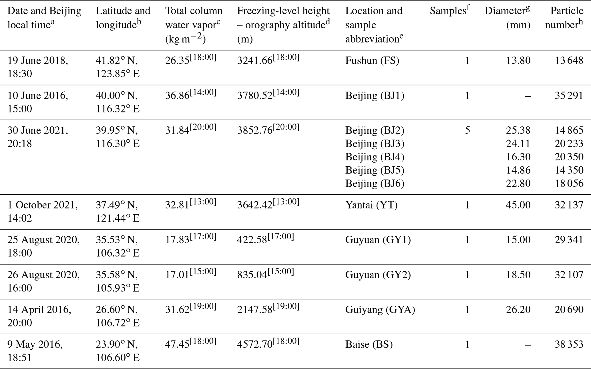
a Date and Beijing local time of hailstorm occurrences. Hailstones were collected within 30 min during hail. b Latitude and longitude where the hailstone were collected. c Total column water vapor values (Beijing local time of ERA5 reanalysis data in square brackets; Hersbach et al., 2018). d Depth between freezing level and orography (Beijing local time of ERA5 reanalysis data in square brackets; Hersbach et al., 2018). e Location and sample abbreviations. f Numbers of hailstones used in the experiments. g Diameter of hailstones (– means no record). h Insoluble particle number in hailstones.
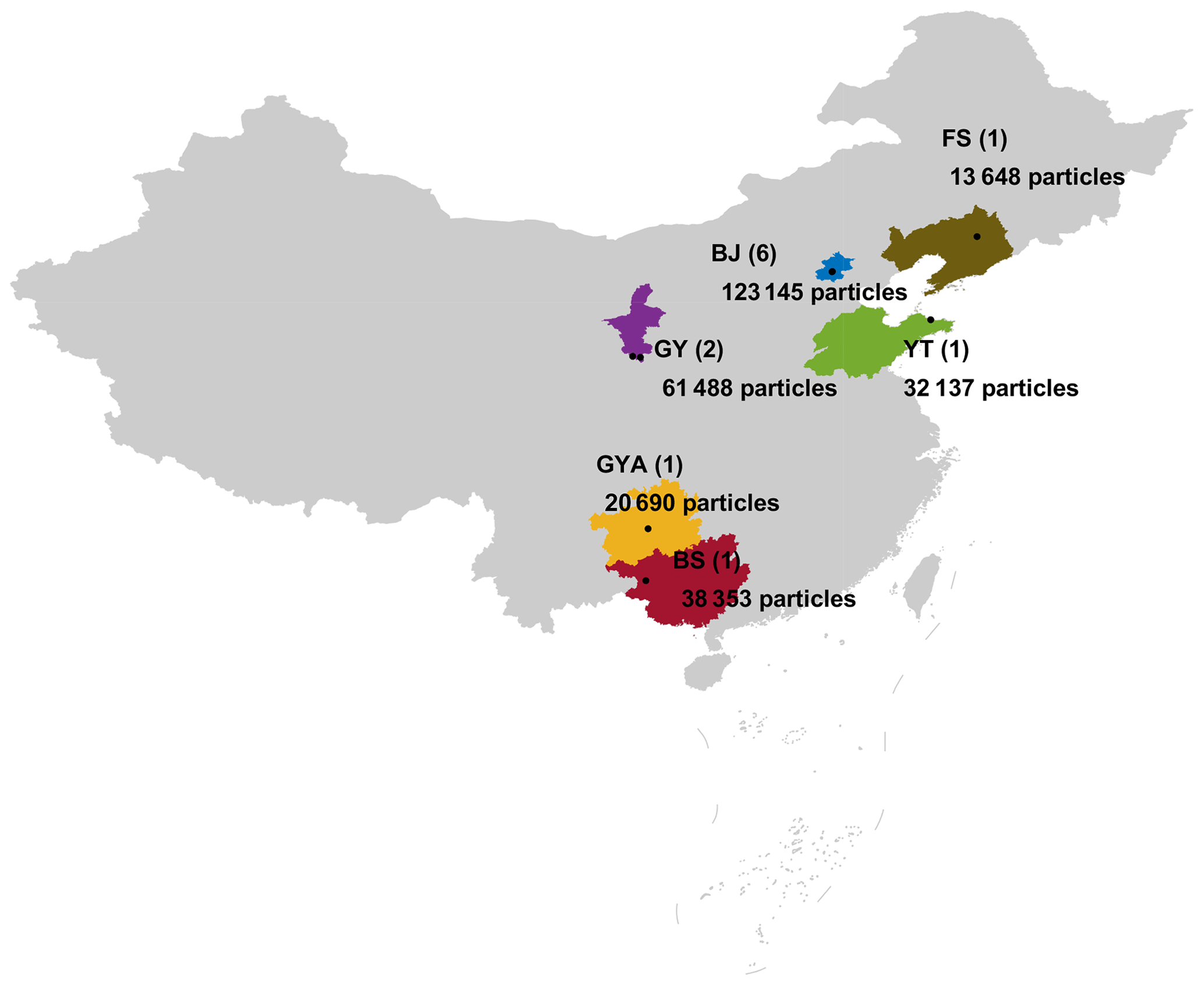
Figure 1Geographical distribution of collected hailstones. The collection locations of the hailstones are indicated by black dots. Provinces of China from which the hailstones were collected are represented by six different colors. The number of hailstones we analyzed was indicated in parentheses. Abbreviations (corresponding to Table 1): BJ – Beijing; BS – Baise; FS – Fushun; GY – Guyuan; GYA – Guiyang; YT – Yantai. Publisher's note: please note that this figure contains disputed territories.
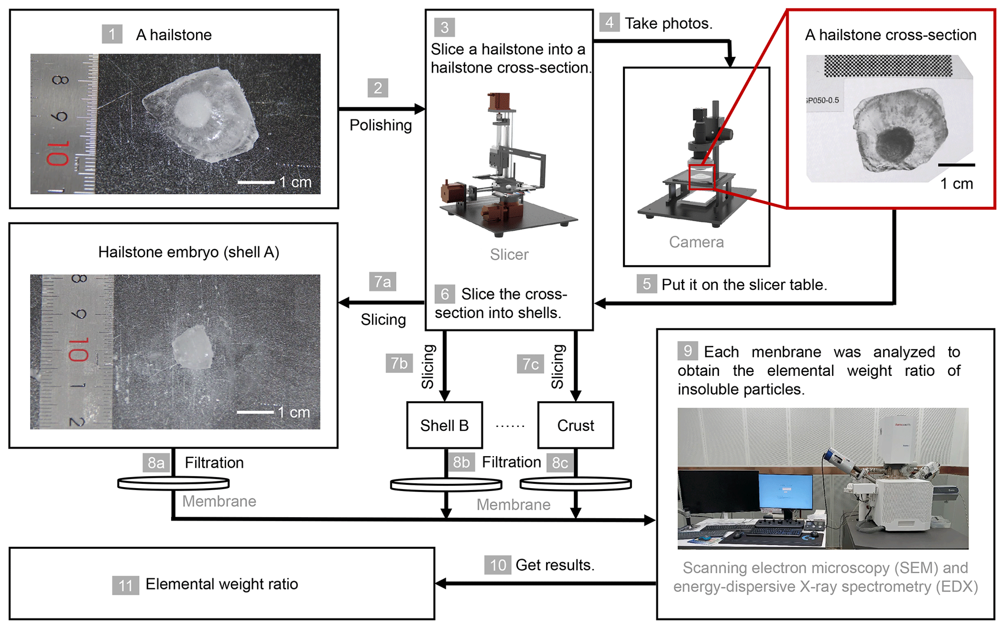
Figure 2Schematic diagram illustrating the experimental framework. (1–2) The surface of each hailstone was polished to remove any attached grass or soil. (3) Subsequently, the hailstones were sliced into cross-sections along the major axis, corresponding to the size of the hailstone embryo. (4–7) After photographing the hailstone cross-sections, they were further subdivided into shells using heated Fe–Cr alloy wire at an air temperature below −8 ∘C. The shells were distinguished based on their natural transparency or opacity. (8) The solution of melting shell samples was then passed through a filter membrane to isolate the insoluble particles. (9) Each shell sample underwent analysis using scanning electron microscopy and energy-dispersive X-ray spectrometry to determine the elemental weight ratios of the insoluble particles within approximately 4 h. (11) Finally, the elemental weight ratio information of hailstones was obtained.
Insoluble particles were extracted in the experiments (Fig. 2). The surface of each hailstone was polished to remove any attached grass or soil. Subsequently, the hailstones were sliced into cross-sections along the major axis, corresponding to the size of the hailstone embryo. The cross-sections were further sliced into shells using heated Fe–Cr alloy wire at an air temperature below −8 ∘C. The shells within a hailstone were distinguished based on their natural transparency or opacity. However, hailstones with a major axis < 7 mm could not be sliced due to the mass loss resulting from heating using our experimental apparatus.
The shells were sequentially labeled with capital letters in alphabetical order, starting from the embryo (designated as shell A) and progressing toward the crust. After the ice shells were melted into a solution, the solution was filtered through a membrane (VSWP01300, Merck KGaA, Germany) with a pore size of 30 nm. The 1 mL (a total of 5 mL) of distilled water underwent five passes through the filter membrane to ensure maximum retention of insoluble particles on the membrane. Subsequently, the filter membrane was dried under an air temperature of approximately 40 ∘C to satisfy the dry-environment requirements of SEM.
The number of insoluble particles in each shell was determined using scanning electron microscopy (SEM), with a focus on particles larger than 0.16 µm. The length along the major axis of the particles was measured using Aztec software (Aztec Software, Oxford Instruments plc, UK) on SEM images. The software was able to randomly capture electron microscopy photos of the membrane (Aztec User Manual, 2013). No particle will be counted repeatedly. Energy-dispersive X-ray spectrometry (EDX) was utilized to determine the elemental weight ratios of the particles. Only elements with an atomic number greater than 4 could be detected due to the X-ray input window being made of beryllium. Each shell sample was analyzed within approximately 4 h by SEM and EDX. The scanning mode of SEM was set in a random order to reduce errors caused by bias in the detection area.
2.2 Clustering and classification
The number of insoluble particles was measured using Aztec on SEM images, but the species could not be determined directly and were identified by a machine learning method. The criteria of species classification were established by the SOMs method to determine the species of unclassified particles. These labeled particles were then regarded as the training set in the random forest classifier. Details are presented in Fig. 3.
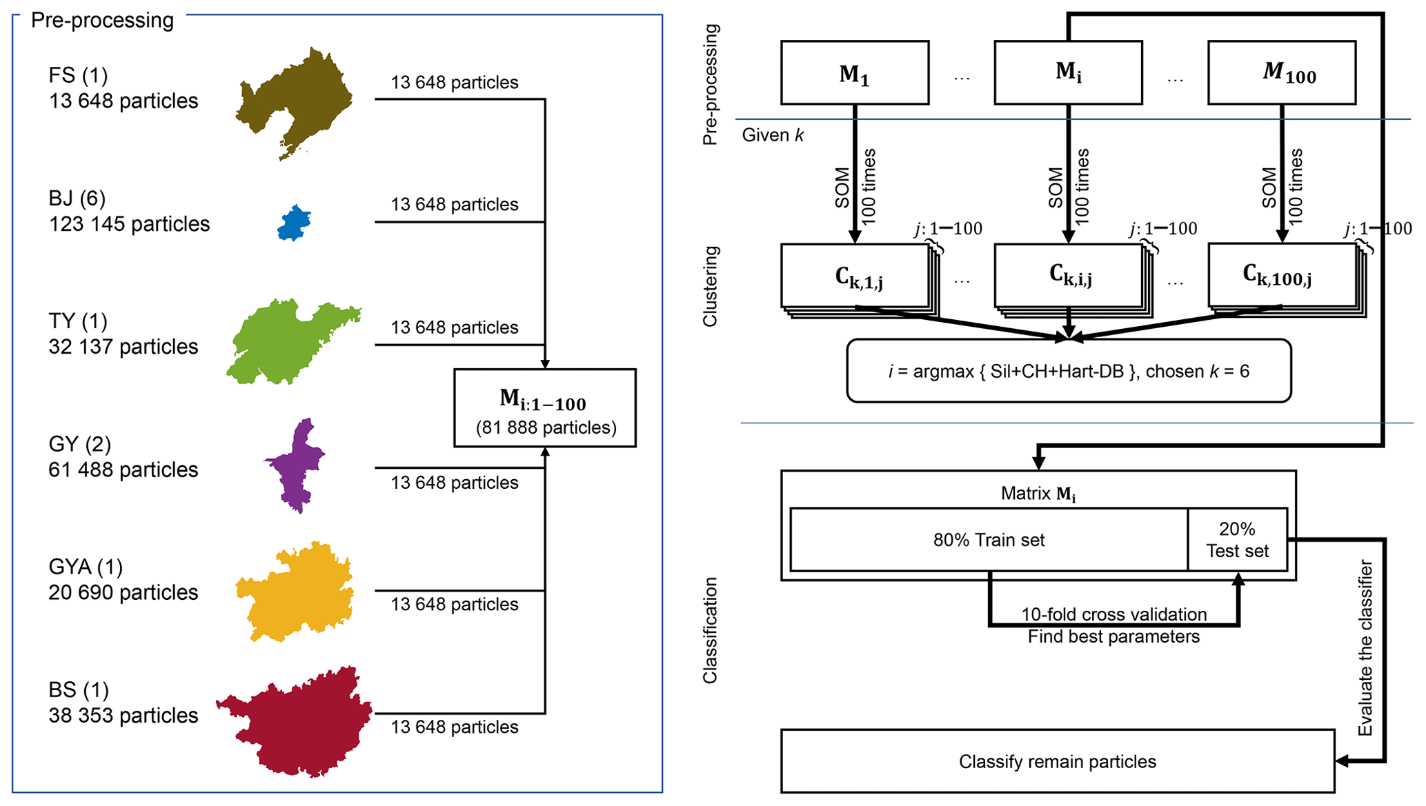
Figure 3Schematic diagram illustrating the methodological framework used for particle identification in this study. A total of 100 matrices Mi, with i ranging from 1 to 100, were utilized in self-organized-maps clustering analyses, each containing 81 888 unidentified particles with 19 elemental features (N, Na, Mg, Al, Si, P, S, Cl, K, Ca, Ti, Cr, Mn, Fe, Ni, Cu, Br, Ba, and Pb). The centroid matrix represents the clustering results obtained through the self-organized-maps method with a given cluster number k. The self-organized-maps operation with the same k was repeated 100 times to ensure result robustness, where j denotes the number of repetitions ranging from 1 to 100. Four indices – silhouette index (Sil), Calinski–Harabasz index (CH), modified Hartigan index (Hart), and Davies–Bouldin index (DB) – were employed to determine the optimal parameters k, i, and j. The matrix Mi containing the identified 81 888 particles was randomly divided into a training set (80 %) and a test set (20 %) for random forest classification. The 10-fold cross-validation was utilized to determine the best tree. Abbreviations (corresponding to Table 1): BJ – Beijing; BS – Baise; FS – Fushun; GY – Guyuan; GYA – Guiyang; YT – Yantai.
With reference to the studies of Ault et al. (2012) and Kirpes et al. (2018) and considering the results of elemental weight ratios determined by EDX analysis, 19 elements (N, Na, Mg, Al, Si, P, S, Cl, K, Ca, Ti, Cr, Mn, Fe, Ni, Cu, Br, Ba, and Pb) were selected to confirm the species of the particles. C and O were not taken in account when clustering or classifying particles as the membrane filters were made from cellulose acetate and cellulose nitrate, which contain C, H, N, and O. We could not detect H because the ray input window was made of beryllium. All particles showed high contents of C and O but different contents of N; thus, N was retained as a feature of classification.
Species of aerosol particles vary with sampling location (Tao et al., 2017). Therefore, when establishing the matrices of elemental weight ratios for clustering, equal amounts of data were randomly extracted from the sample data from each province to ensure the inclusion of a consistent proportion of samples from each region in the training process. A hailstone from FS (collected from Fushun City, Liaoning Province) was shown to contain 13 648 insoluble particles, which was the smallest amount among all samples from six provinces (Fig. 1). With random sampling of 13 648 particles from each province, the matrix used in clustering analyses included 81 888 particles. This operation was repeated 100 times to obtain 100 matrices Mi with i ranging from 1 to 100.
Each matrix Mi was clustered using the SOMs method. SOMs belong to the category of competitive learning algorithms and are a type of artificial neural network (Kohonen, 1990). A basic SOMs network consists of an input layer, weight vectors, and an output layer. Each neuron in the output layer possesses a set of weight vectors, which represent the topological structure of the neurons in the output layer, associated with the inputs. SOMs are commonly used as dimensionality reduction algorithms, enabling the representation of high-dimensional data in a lower-dimensional structure while preserving the original topology. When SOMs are trained on unlabeled data for clustering purposes, it proves to be highly beneficial in clustering unlabeled and high-dimensional inputs into visualized two-dimensional outputs.
We utilized the SOMs code from MATLAB's deep learning toolbox. The input of SOMs is Mi. At the beginning, the neural network in the output layer was initialized as a 1-D dimension with k neurons. The number of neurons in the output layer matches k ranging from 2 to 10. The operation of SOMs with the same initialized k neurons and input matrix Mi was repeated 100 times to ensure result robustness. The clustering result was stored in matrix , which corresponded to the given k centroids in Mi with jth SOMs operation. Each matrix consists of k rows and 19 columns (corresponding to the number of elemental features). Four indices, namely, the silhouette index (Rousseeuw, 1987), the Calinski–Harabasz index (Calinski and Harabasz, 1974), the modified Hartigan index (de Amorim and Hennig, 2015; Hartigan, 1975), and the Davies–Bouldin index (Davies and Bouldin, 1979), were selected as evaluation indicators to determine the parameters k, i, and j. The silhouette index, Davies–Bouldin index, and Calinski–Harabasz index assess the similarity between a particle and others within the same cluster, as well as the dissimilarity across different clusters for a given k. The Hartigan index evaluates whether it is worthy to increase the k. Notably, the Hartigan index has undergone modifications that preserve its statistical meaning while conserving computational resources.
The Hartigan index (de Amorim and Hennig, 2015; Hartigan, 1975) is defined as follows:
where k is the number of clusters, N is the number of observations, Cg is the centroid of cluster g, and xg is the observation of cluster g.
The calculation of H(k) requires clustering for values of k ranging from 2 to 11 in order to obtain H(2), H(3), …, H(10). Clustering particles into 11 clusters would require performing an additional 10 000 iterations of the SOMs, with 100 iterations of extracting Mi and 100 iterations of SOMs for each Mi. Additionally, we observed that the SOMs did not perform well in the silhouette index (Sil), the Calinski–Harabasz index (CH), and the Davies–Bouldin index (DB) when k=2. As a result, we introduced modifications to the Hartigan index.
When k=1, it indicates that all particles belong to one cluster.
where C is the centroid of all data and xn refers to the observation of data. In clustering with a specific value of k, our objective is to have particles tightly grouped together in feature space while ensuring that the centroids exhibit a significant dispersion compared to k−1. A higher value of Hart(k) for a given k indicates improved clustering performance. The best k, i, and j were chosen by combining the evaluation of the four indices (Fig. 4). We applied max normalization to rescale the four indices, Sil(k), CH(k), DB(k), and Hart(k). Subsequently, the best combination of k, i, and j was determined, resulting in , reaching its maximum.
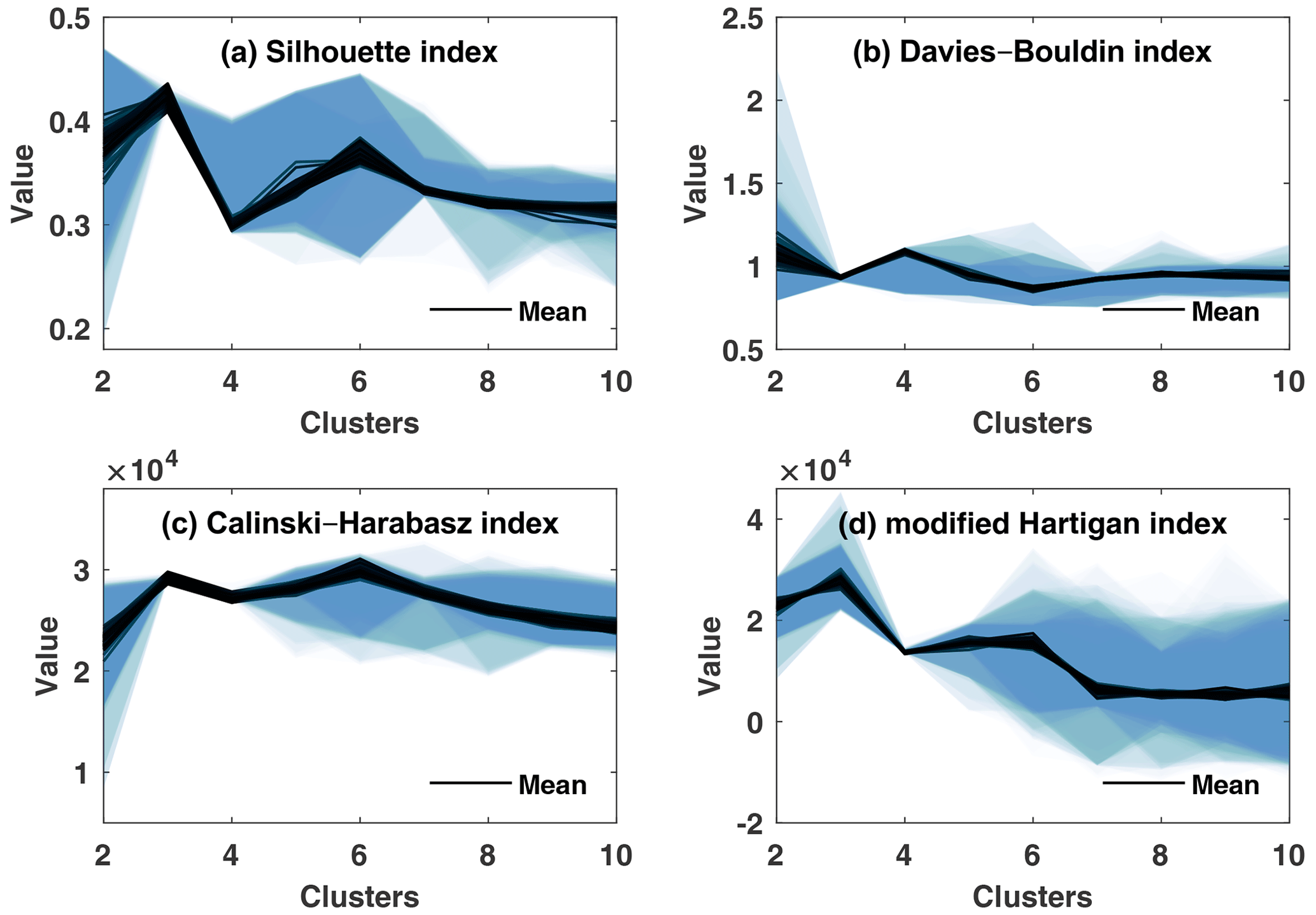
Figure 4Evaluation of self-organized-maps clustering results. The clustering results of self-organized maps were evaluated using (a) the silhouette index, (b) the Davies–Bouldin index, (c) the Calinski–Harabasz index, and (d) the Hartigan index. The self-organized-maps operation was repeated 100 times to ensure result robustness. The solid lines and shading represent the average and spread of 100 repetitions, respectively.
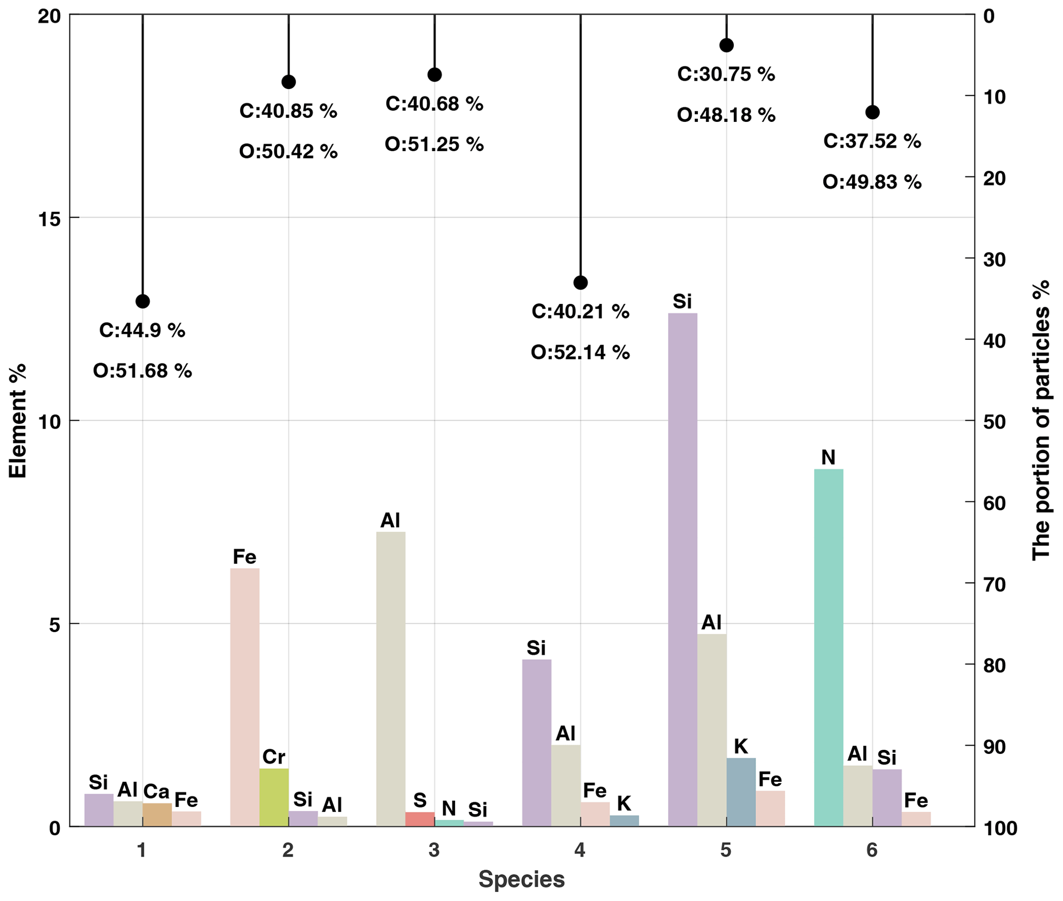
Figure 5Centroids of clustering with six clusters from self-organized-maps results and each species portion. Colored bars show the top four elements of each species. The stem bars show the portion of each species. The average contents of C and O of each species are marked at the end of the stem bars.
The centroid matrix with the best k, i, and j was treated as an instruction for random forest classification. The chosen centroid matrix with the top four elements is shown in Fig. 5 with k=6. The first species with a low elemental weight ratio, except for C and O contents, was considered to be organics. The second species with high Fe content and low Cr content was introduced by the material of the slicer used in the experiment. The third species had a high Al content, representing oxides or carbonates of aluminum. The fourth and fifth species were mineral silicates. Thus, the third, fourth, and fifth species were referred to as dust. The last species with high N content was protein-containing biological aerosol.
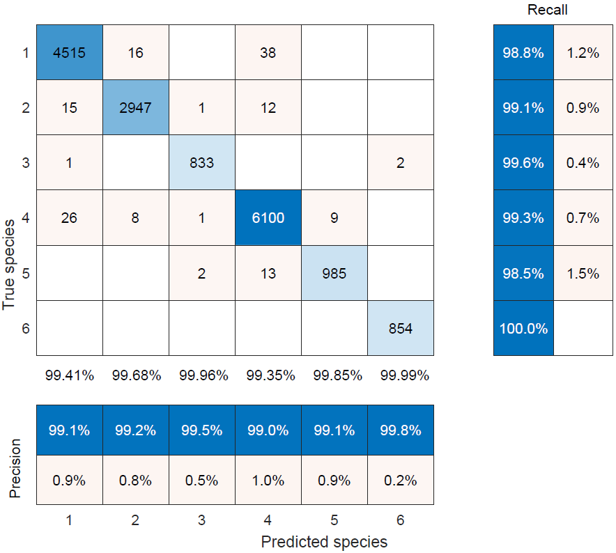
The random forest method was applied in classifying insoluble particles, which involves randomly growing 100 classification trees. The training set consisted of 80 % of particles of Mi, and 10-fold stratified cross-validation was applied during the training process to find the best tree among the 100 random trees. The remaining 20 % of particles of Mi were used as the test set to evaluate the best tree. The confusion matrix of classification results is shown in Table 2. All remaining insoluble particles were classified by this tree. Finally, we identified three species: organics, dust, and bioprotein aerosols.
Table 2Confusion matrix of the best random forest classifier tree. The numbers on the diagonal are accurately predicted insoluble particles. Numbers in bold indicate the accuracy of the prediction of each type.
2.3 Conversion of insoluble particle number concentration
Particle number was converted to a number concentration per cubic centimeter volume water (hereinafter referred to as number concentration) using the following formula:
The number of insoluble particles in the melted-shell solution (Nliquid) can be calculated by multiplying their number concentration (nliquid) with the volume of the shell solution (Vliquid). Part of the solution was not used up in the experiments and was kept as a backup. Therefore, the shell solution was diluted in some experiments, and part of the solution was consumed in the experiments. As in the melting solution, the number of insoluble particles in the diluted solution (Ndiluted) can be calculated by multiplying their number concentration (ndiluted) with the volume of the diluted solution (Vdiluted). The total particle number in the melted shell (Nliquid) remains unchanged during the dilution process (Ndiluted).
The number concentration of the diluted solution (ndiluted) is equal to that of the consumed part (nused). Assuming that the rinsing operation ensures all insoluble particles in the shell were on the membrane, the number of insoluble particles in the consumed solution (Nused) is equal to the number of insoluble particles counted on the membrane (Nfilter).
We use SEM to capture electron microscopy images of the membrane. Assuming a uniform distribution of insoluble particles on the filter membrane, software randomly captured electron microscopy photos of the membrane and counted the visible insoluble particles in those images. The relationship between the total number of visible insoluble particles counted in the images (Ncount) and Nfilter is as follows:
That is, Nfilter is determined by multiplying Ncount by the ratio of the areas between the entire filter membrane (Sfilter) and the electron microscopy images (Simages). These three formulas (Eqs. 6–8) were reduced to Eq. (9):
Here, Sfilter, Simages, Ncount, Vdiluted, and Vused can be measured. The liquid volume (Vliquid) was determined as the average of readings obtained by two experimenters from the test tube. Take the logarithm on both sides:
Based on Eq. (10), a tiny change in nliquid can be represented as dnliquid:
where
The uncertainty (Δ) of nliquid comes from the measurement error of the experimental instruments, following the below (Taylor, 1997):
Here, the accuracy of the test tube is 0.1 mL. The term dV represents the greatest reading error caused by humans and was set to 0.05 mL. The quantity corresponds to the uncertainty associated with the size of insoluble particles and the scan settings.
The term dPs represents the minimum number of pixels that can be detected in an image. Ps denotes the total number of pixels in the micrograph.
2.4 Curve fitting
We aggregated insoluble particles into 0.2 µm intervals (0.2 µm bin interval in Figs. 6 and 9 and 2 µm bin interval in Figs. 7 and 8) to fit the logarithmic normal distribution:
N denotes the total number concentration of particles. Both n(ln D) and n(D) represent the size distributions of particles, where D is the diameter of insoluble particles. n(ln D) and n(D) can be converted to each other by D.
When the Ncount in an interval equals 1, the number concentration will exhibit a flat tail due to the conversion to obtain nliquid. The fitting data were selected with intervals equal to 0.2 µm. The least-squares method was applied to determine the fitting parameters, and R2 was used to estimate the goodness of fit. The two centroids of the fitting parameters of organics and dust were determined by the K-means method.
A total of 289 461 insoluble particles were detected from 30 shells of 12 hailstones using SEM. The identification of insoluble particles employed SOMs for clustering and random forest for classification. Four indices were utilized to determine the appropriate parameters in clustering. The clustering results were divided into a training set and a testing set for classification. The confusion matrix of the best classifier showed an accuracy, precision, and recall of 99.7 %, 99.3 %, and 99.2 %, respectively. All particles were classified as organics, dust, and bioprotein aerosols (i.e., the fraction of biological aerosols with protein content).
3.1 Sample similarity
Five of the 12 hailstones (BJ2–BJ6) were from the same hailstorm that occurred in Beijing on 30 June 2021. The insoluble particles present in BJ2–BJ6 showed similarity in the size distribution of organics, dust, and bioprotein aerosols, while those from eight hailstones (BJ1, BJ2, BS, FS,GY1, GY2, YT, and GYA) exhibited a wider dispersion (Fig. 6). The results were similar to those of Li et al. (2018), who reported that the number concentrations of water-soluble ions varied among hailstorm events but showed similarity in the same storm (Li et al., 2018). These analyses suggested that insoluble particles in the hailstorm may come from local natural or anthropogenic emissions (e.g., soil dust, aerosols from biomass and fossil fuel combustion, and/or products of the conversion of gaseous precursors), which is also suggested by the results for water-soluble ions (Beal et al., 2022). The updraft within the hailstorm is likely to bring insoluble particles from local surfaces or boundary layers into deep-convective clouds as hailstorms are among the most severe storms with strong updrafts (Battaglia et al., 2022).
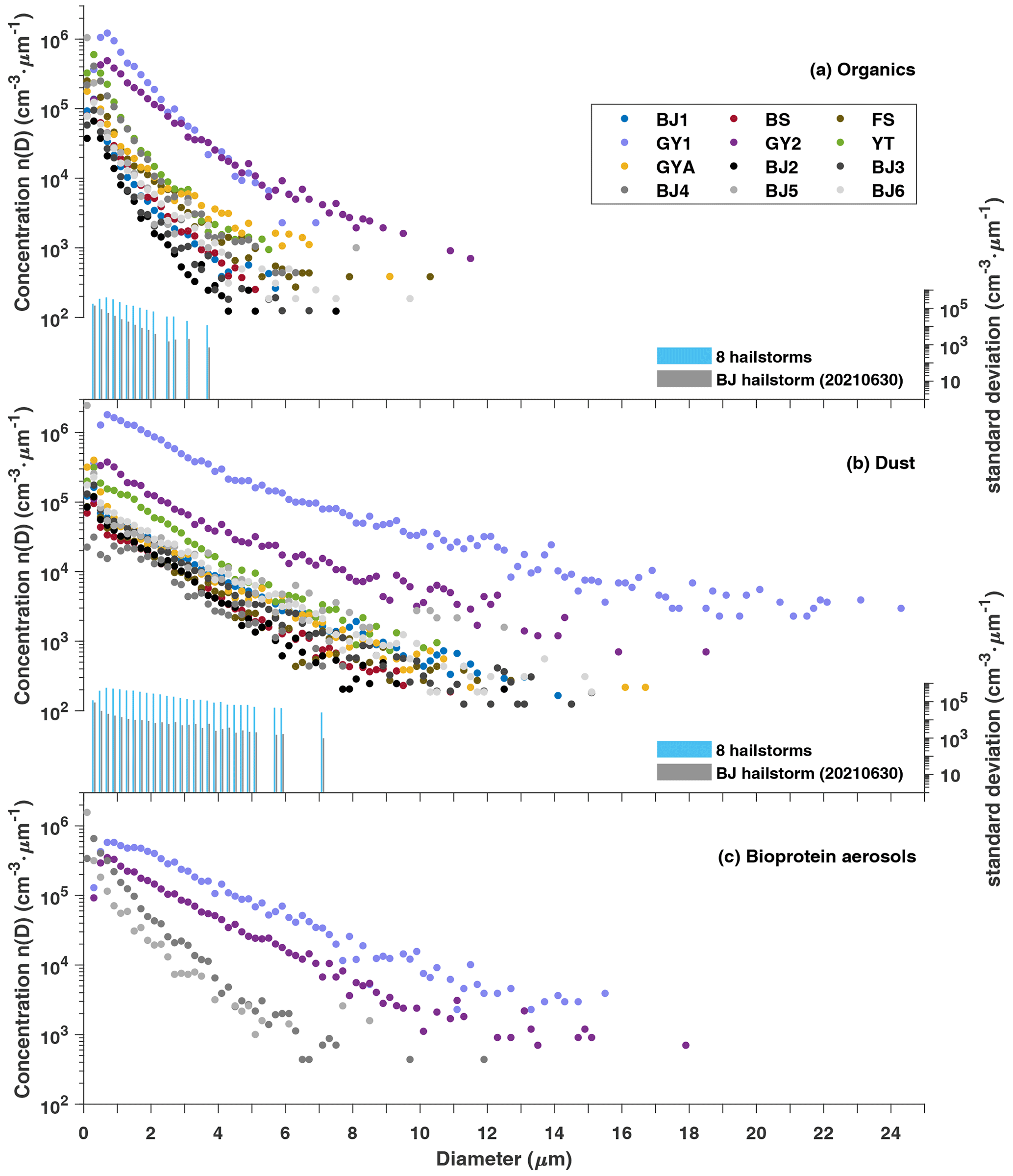
Figure 6Size distribution of (a) organics, (b) dust, and (c) bioprotein aerosols of insoluble particles in 12 hailstones. The colored dots represent data from seven hailstones (BJ1, BS, FS,GY1, GY2, YT, and GYA) which were from different hailstorms. The black and gray dots correspond to data from hailstones (BJ2 to BJ6) that were from the same hailstorm that occurred in Beijing on 30 June 2021. The blue and gray bars indicate the standard deviation of the number concentration of insoluble particles from eight hailstones (BJ1, BJ2, BS, FS,GY1, GY2, YT, and GYA) from eight cases and five hailstones (BJ2 to BJ6) from one case, respectively. Abbreviations (corresponding to Table 1): BJ – Beijing; BS – Baise; FS – Fushun; GY – Guyuan; GYA – Guiyang; YT – Yantai.
3.2 Size distribution in embryos
All hailstone embryos analyzed in this study are graupel particles, which grow from the initial ice particles through accretion of supercooled droplets (Knight, 1981). These initial ice particles are formed through nucleation of insoluble particles where heterogeneous nucleation takes place (Lamb and Verlinde, 2011). In other words, insoluble particles in graupels influence the formation of ice crystals and subsequently affect the formation of hailstone embryos.
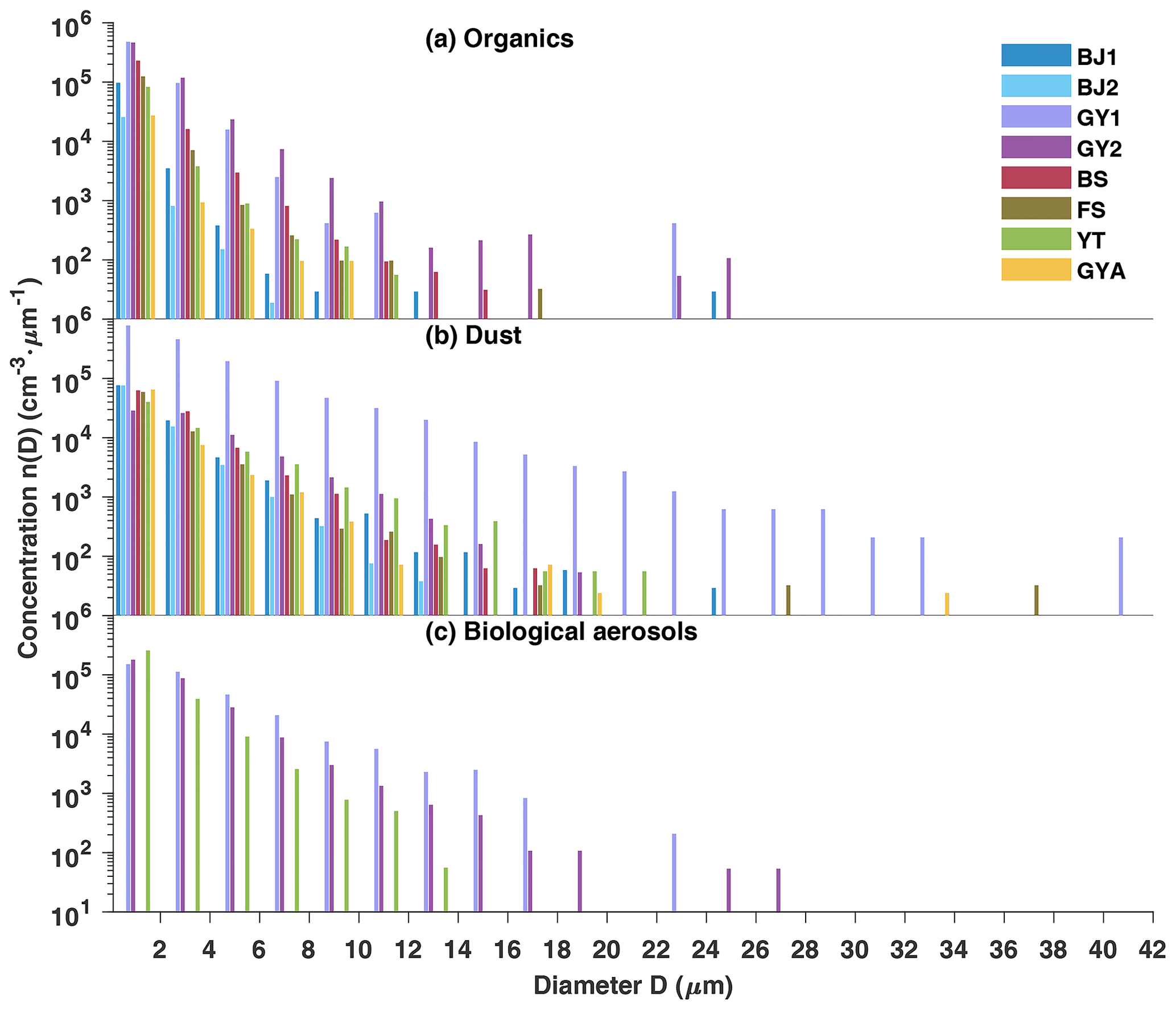
Figure 7Size distribution of (a) organics, (b) dust, and (c) bioprotein aerosols in hailstone embryos. Colors represent different hailstones. Abbreviations (corresponding to Table 1): BJ – Beijing; BS – Baise; FS – Fushun; GY – Guyuan; GYA – Guiyang; YT – Yantai.
The variations in number concentrations of dust and bioprotein insoluble particles indicate that particle number concentrations decrease exponentially with particle diameter, with markable variation observed among hailstorms (Fig. 7). BJ2 was selected to represent five hailstones from the same storm to simplify comparison. The size distribution distinguishes organics from dust and bioprotein aerosols. The number concentrations of organics from all samples decrease with particle diameters less than 8 µm, while those of GY1 and GY2 fluctuate starting at diameters of 8 and 12 µm, respectively. Compared to other hailstones, GY1 and GY2 were collected in remote areas, where there are fields of rural areas dedicated to growing crops near the south of the Gobi Desert. Therefore, GY1 and GY2 have a coarse mode of organics with particle diameters larger than 12 µm, possibly due to the emission of spring wheat straw burning and unrestricted diesel engine vehicles. The transport of coal combustion in surrounding cities may also contribute to the coarse-mode organics. Among all cases, there is a significant variance in the size distribution of both organics and dust. The number concentration of organics from a hailstone embryo varied from 1 to 390 times compared to those at the same particle diameter in hailstone embryos from different cases. The number concentration of dust from a hailstone embryo varied from 1 to 527 times compared to those at the same particle diameter in hailstone embryos from different cases. The number concentrations of dust from BJ1, BJ2, and GY1 are at least 3 times higher than those of organics in particles of the same diameter in the range of 2–24 µm.
Moreover, dust showed a wider size distribution than organics and bioproteins among all samples. Dust from GY1 had a higher number concentration and a larger maximum size (42 µm) compared to other hailstone embryos. Hailstone samples with high insoluble particle content, i.e., GY1 and GY2, showed significantly lower total column water vapor values and smaller depths between freezing-level height and orography within 1 h before hailstorm occurrence compared to other hailstones (Table 1). The competition between condensation and the relatively shorter updraft pathway might be responsible for the high number concentrations of organics, dust, and bioproteins in GY1 and GY2 as compared with other hailstones. Bioprotein aerosols, with high freezing efficiency, may have formed initial ice particles in GY1, GY2, and YT, while dust or organics formed initial ice particles in hailstorms in the other five cases. All hailstone embryos contained organics and dust, but not all hailstone embryos contained a significant amount of bioprotein aerosols. Due to limited comprehension of the transportation and transformation processes of biological materials, it is challenging to establish a definitive relationship between biological protein particles and biological aerosols (Fröhlich-Nowoisky et al., 2016).
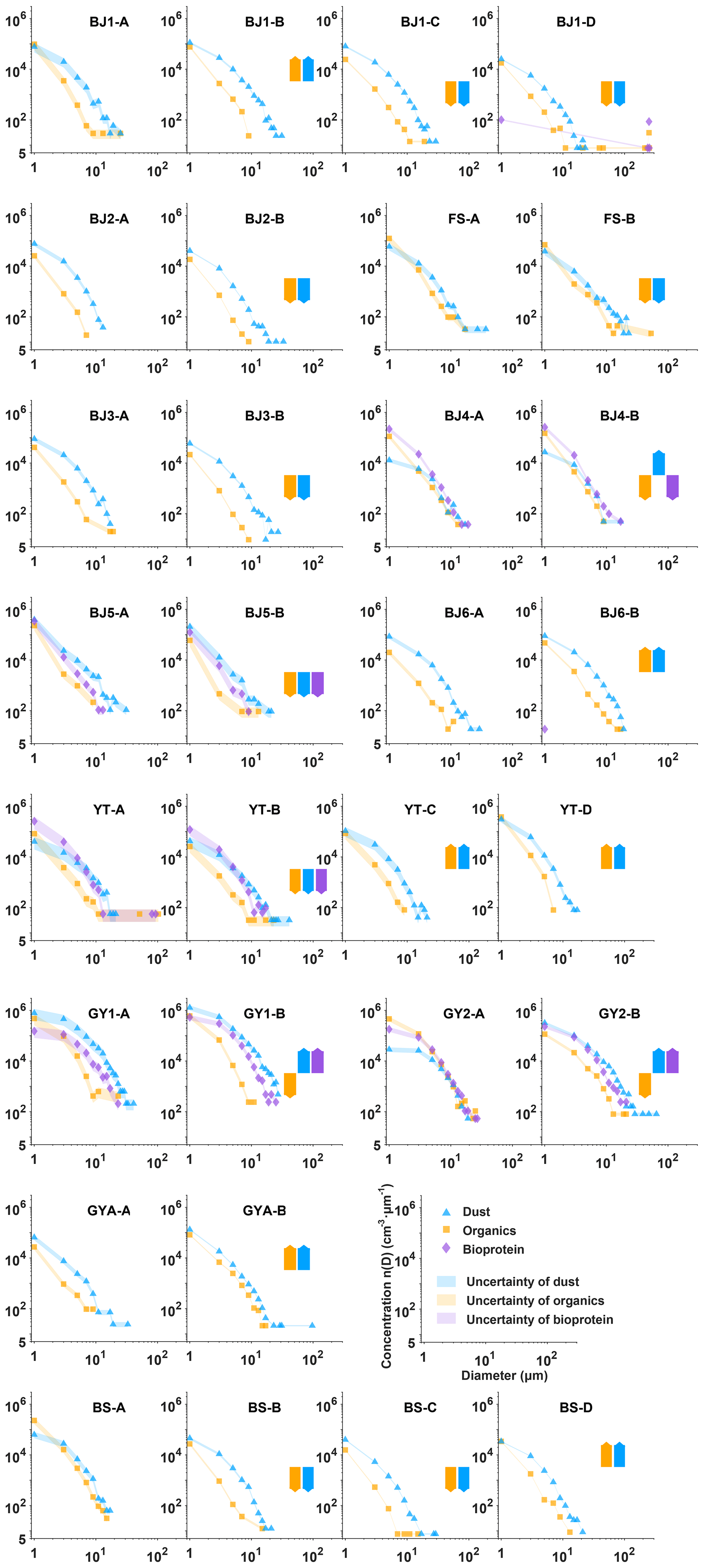
Figure 8The size distribution of insoluble particles within the natural shells of 12 hailstones is represented. Blue triangles, orange squares, and purple diamonds are used to indicate dust, organics, and bioprotein aerosols, respectively. The natural shells are denoted alphabetically with capital letters (shell A refers to embryos, and shell B–D refers to the crust of hailstones). The arrow direction illustrates the tendency of particle number concentration in each layer compared to the previous shell. Shading is employed to indicate uncertainty. Detailed calculations are provided in Sect. 2.3. Abbreviations (corresponding to Table 1): BJ – Beijing; BS – Baise; FS – Fushun; GY – Guyuan; GYA – Guiyang; YT – Yantai.
3.3 Size distribution in shells
The size distributions of each species varied little in terms of characteristics between outer shells with the embryos (Fig. 8). In a four-shell hailstone, the number concentrations of insoluble particles exhibited V-shaped distributions (BS and YT) or inverse V-shaped distributions (BJ1) from embryo to crust. Five out of nine two-shell hailstones showed higher number concentrations of dust in crusts than in embryos, while seven of them showed higher number concentrations of organics in embryos than in crusts. Moreover, the quantification of differences in number concentration varied little among shells. The 90.5 % points showed that differences in the number concentration of the same kinds of particles in a shell compared to those of the previous shell at the same diameter were within a factor of 2 (294 data points in Fig. 8). This observation is attributed to the fact that the growth of hailstones beyond the embryo stage relies on the accretion of supercooled water rather than ice crystals (Lamb and Verlinde, 2011). Consequently, the hailstone record not only insoluble particles during the embryo formation but also insoluble particles in the hailstone growth zone throughout the hailstorm. As a result, the size distribution of particles within all of the hailstones may represent the distribution of insoluble particles in deep-convection regions through which the hailstones went.
3.4 Logarithmic normal distribution of dust and organics
The size distributions of dust and organics in the whole hailstone can be described by a logarithmic normal distribution (Fig. 9) (Lamb and Verlinde, 2011):
where n(ln D) is the number concentration of insoluble particles per cubic centimeter volume water ranging from to . Here, D represents the diameter of particles (in micrometers), ln Dg is the geometric mean diameter, and ln σg is the geometric standard deviation (Lamb and Verlinde, 2011). The number of bioprotein aerosols was below the limit of detection in some samples so that only the curves of organics and dust were fitted. The fitting parameters of the same species were aggregated in parameter space and were suspected to be related to the physical properties of each species, requiring further studies for confirmation. Moreover, the fitting parameters of organics and dust particles were clustered into two centroids (Fig. 9) by the K-means method, which indicated that organics and dust have two classic modes (classic mode of organics: , ln σo=0.91, and cm−3; classic mode of dust: ln Dd=0.11, ln σd=1.07, and cm−3). That is, insoluble organics in hailstones are usually smaller in diameter and present in lower amounts than dust. Regardless of fine or coarse particles (particles D < 0.5 µm in diameter were not considered in reference to DeMott et al., 2010), the number concentration of dust was up to 2 orders of magnitude higher than the number concentration of organics. These observations indicated that dust accounted for the major portion of particles in eight hailstorms (not considering bioprotein), which was consistent with the observations of embryos described above.
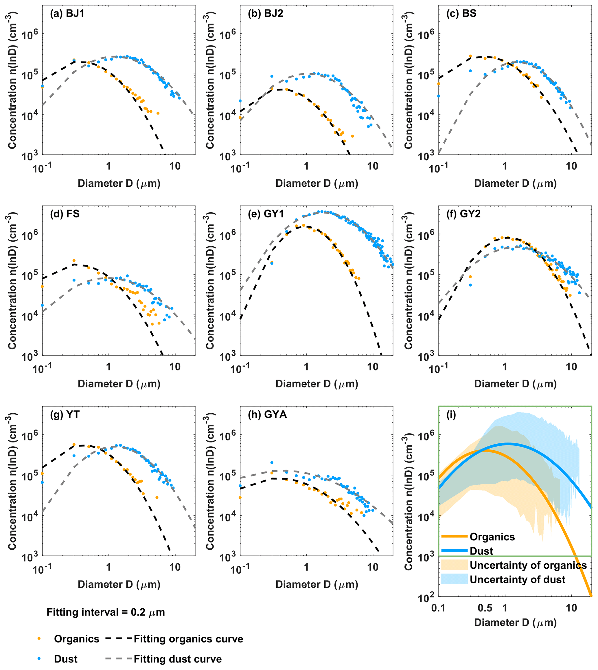
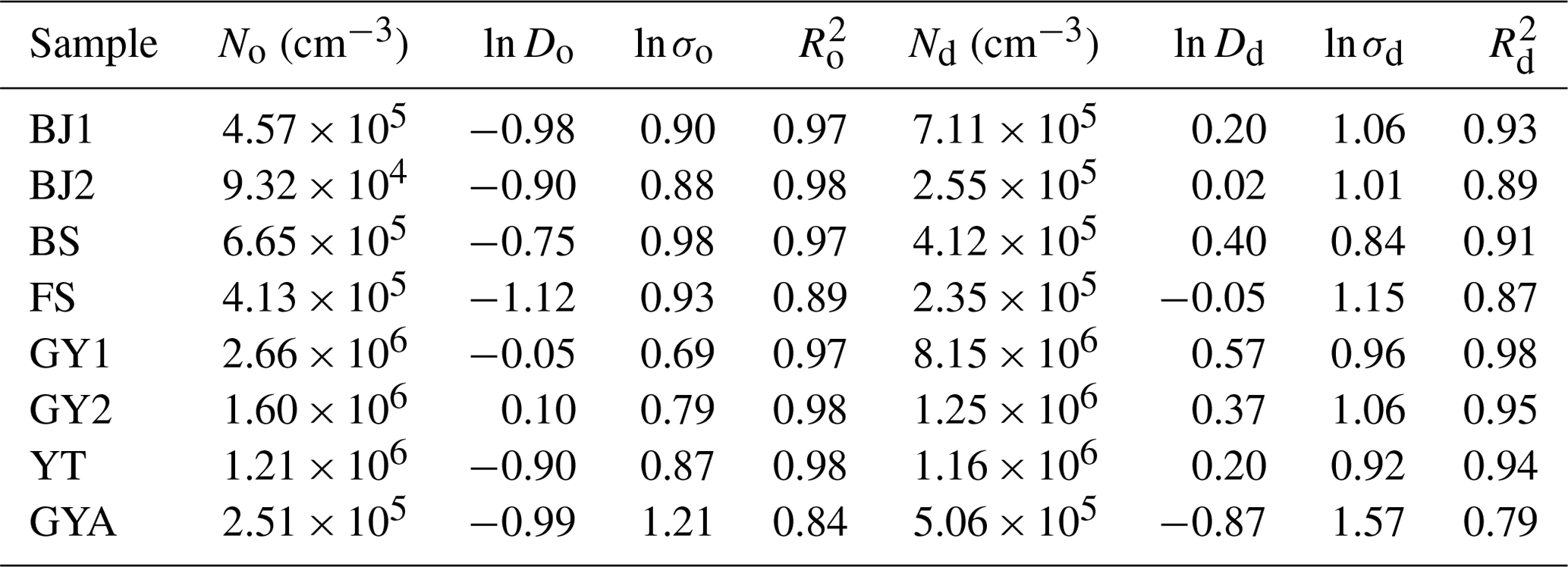
Figure 9Fitting size distribution functions of organics and dust contained in the whole hailstone. (a–h) Fitting parameters of logarithmic normal distributions of BJ1, BJ2, BS, FS, GY1, GY2, YT, GYA. (i) Classic modes of dust and organics (interval of data is 0.2 µm, and fitting curves are painted with intervals of 0.02 µm). The fitting parameters for panels (a)–(h) are listed in Table 3. The fitting range of (a)–(h) is shown with a green rectangle in (i). The centroid of the organics' fitting parameter (orange line) is ln σo=0.91, , and cm−3. The centroid of the dust fitting parameter (blue line) is ln σd=1.07, ln Dd=0.11, and cm−3. Shading shows uncertainty of organics and dust. Abbreviations (corresponding to Table 1): BJ – Beijing; BS – Baise; FS – Fushun; GY – Guyuan; GYA – Guiyang; YT – Yantai.
Table 3The fitting parameters of dust and organics size distributions in Fig. 9a–h.
This was the first study to simultaneously analyze both the number concentrations and species (including organics, dust, and bioproteins) of insoluble particles in hailstones. The findings from this analysis offer valuable insights into particle observations within severe storms. Understanding the number concentration and composition of these insoluble particles is crucial as they play a significant role as ice-nucleating particles during the heterogeneous nucleation process in deep convection.
The size distribution of insoluble particles in hailstones from the same hailstorm showed less variation than those from different hailstorms. One possible reason is that updrafts of hailstorms brought insoluble particles from local surfaces or boundary layers into deep-convective clouds. Moreover, almost all insoluble particles in hailstone embryos analyzed in this study showed an exponential size distribution, which was consistent with the effects of gravity. The number concentrations of organics and dust from different hailstone embryos differed by up to 389 times and 526 times at the same diameter, respectively. The changes in particle concentration may lead to at leat 1-order-of-magnitude variance in ice-nucleating particles (DeMott et al., 2010). Additionally, the size distribution of insoluble particles varied in shells by up to 27 times, which was much smaller than differences between different hailstorms.
Two logarithmic normal distribution models were applied to fit the size distribution of organics and dust within hailstones, providing a description of insoluble particles in the deep convection during hailstone formation. The analysis of the two classic size distribution modes of insoluble particles indicated a significant presence of dust without considering bioprotein. Furthermore, a positive correlation exists between the number concentrations of insoluble particles and those of ice-nucleating particles in hailstones, specifically for corresponding species (figure not shown). A further measurement of ice-nucleating particles by drop-freezing experiments will establish the relationship between insoluble particles and immersion ice-nucleating particles. The combination of these results with future experiments to determine the number concentrations and species of particles from local observations will establish the relationship between surface observations and ice-nucleating particles in deep-convective clouds, which will lead to an improvement in the parameterization of ice-nucleating particles in both weather and climate models.
Nonetheless, two kinds of classic size distribution modes of organics and dust in hailstones were performed, but a more robust classic mode required a larger number of samples. In future, for climate or weather models, the classic mode can be assumed as the mean state to describe the characteristics of insoluble particles in supercooling water. In addition, this study did not attempt to parameterize bioprotein aerosols because there was a great uncertainty in quantification due to a poor understanding of biological processes (Fröhlich-Nowoisky et al., 2016). Further collaborative studies are required to gain a better understanding of biological processes to establish the classic bioprotein mode.
The self-organized-maps algorithm, the random forest algorithm, and the 10-fold stratified cross-validation algorithm can be found in the MATLAB Deep Learning Toolbox: https://ww2.mathworks.cn/help/deeplearning/index.html (The MathWorks, Inc., 2022). Identification algorithms are coded in MATLAB and can be made available upon request.
The experimental data can be made available upon request. ERA5 reanalysis data are publicly accessible (https://doi.org/10.24381/cds.adbb2d47, Hersbach et al., 2018).
HZ wrote the original draft for the concept presented by QZ. HZ, XL, and CPN participated in the pre-processing and reservation of hailstones from volunteers. HZ and XL sliced hailstones using machines manufactured by KB and performed the experiments analyzing the element weight ratios of insoluble particles with the help of LC. KB also provided hailstones BJ2–BJ6. Machine learning the on identification of particles was operated by HZ. YR and HX compared ice nucleation particles from drop-freezing experiments with our data. ZC provided hailstones GY1 and GY2. All the authors discussed and contributed to the final paper. QZ directed this project.
The contact author has declared that none of the authors has any competing interests.
Publisher’s note: Copernicus Publications remains neutral with regard to jurisdictional claims made in the text, published maps, institutional affiliations, or any other geographical representation in this paper. While Copernicus Publications makes every effort to include appropriate place names, the final responsibility lies with the authors.
The authors are grateful for the funding support provided by the National Natural Science Foundation of China, the Innovation Project of the China Meteorological Administration, and the Key R&D projects of the Ningxia Hui Autonomous Region. We also wish to thank Cai Yao from the Meteorological Bureau of Guangxi, China, for collecting hailstones at BS in Guangxi and the volunteers who collected hailstones. The authors are grateful to Jiwen Fan from the Pacific Northwest National Laboratory of the United States for the discussions.
This research has been supported by the National Natural Science Foundation of China (grant nos. 42030607 and 41930968) and the Key Research and Development Program of Ningxia (grant no. 2022BEG02010).
This paper was edited by Aijun Ding and reviewed by three anonymous referees.
Ault, A. P., Peters, T. M., Sawvel, E. J., Casuccio, G. S., Willis, R. D., Norris, G. A., and Grassian, V. H.: Single-particle SEM-EDX analysis of iron-containing coarse particulate matter in an urban environment: Sources and distribution of iron within Cleveland, Ohio, Environ. Sci. Technol., 46, 4331–4339, https://doi.org/10.1021/es204006k, 2012.
Aztec User Manual: https://utw10193.utweb.utexas.edu/InstrumentManuals/Oxford%20EDS%20AZtec%20User%20Manual.pdf (last access: 22 August 2023), 2013.
Battaglia, A., Mroz, K., and Cecil, D.: Satellite hail detection, in: Precipitation Science, Elsevier, 257–286, https://doi.org/10.1016/B978-0-12-822973-6.00006-8, 2022.
Beal, A., Martins, J. A., Rudke, A. P., de Almeida, D. S., da Silva, I., Sobrinho, O. M., de Fátima Andrade, M., Tarley, C. R. T., and Martins, L. D.: Chemical characterization of PM2.5 from region highly impacted by hailstorms in South America, Environ. Sci. Pollut. Res., 29, 5840–5851, https://doi.org/10.1007/s11356-021-15952-6, 2022.
Calinski, T. and Harabasz, J.: A dendrite method for cluster analysis, Commun. Stat.-Theory Methods, 3, 1–27, https://doi.org/10.1080/03610927408827101, 1974.
Chen, Q., Yin, Y., Jiang, H., Chu, Z., Xue, L., Shi, R., Zhang, X., and Chen, J.: The Roles of Mineral Dust as Cloud Condensation Nuclei and Ice Nuclei During the Evolution of a Hail Storm, J. Geophys. Res.-Atmos., 124, 14262–14284, https://doi.org/10.1029/2019JD031403, 2019.
Davies, D. L. and Bouldin, D. W.: A Cluster Separation Measure, IEEE Trans. Pattern Anal. Mach. Intell., PAMI-1, 224–227, https://doi.org/10.1109/TPAMI.1979.4766909, 1979.
de Amorim, R. C. and Hennig, C.: Recovering the number of clusters in data sets with noise features using feature rescaling factors, Inf. Sci. (Ny.), 324, 126–145, https://doi.org/10.1016/j.ins.2015.06.039, 2015.
DeMott, P. J., Prenni, A. J., Liu, X., Kreidenweis, S. M., Petters, M. D., Twohy, C. H., Richardson, M. S., Eidhammer, T., and Rogers, D. C.: Predicting global atmospheric ice nuclei distributions and their impacts on climate, P. Natl. Acad. Sci. USA, 107, 11217–11222, https://doi.org/10.1073/pnas.0910818107, 2010.
DeMott, P. J., Prenni, A. J., McMeeking, G. R., Sullivan, R. C., Petters, M. D., Tobo, Y., Niemand, M., Möhler, O., Snider, J. R., Wang, Z., and Kreidenweis, S. M.: Integrating laboratory and field data to quantify the immersion freezing ice nucleation activity of mineral dust particles, Atmos. Chem. Phys., 15, 393–409, https://doi.org/10.5194/acp-15-393-2015, 2015.
Fröhlich-Nowoisky, J., Kampf, C. J., Weber, B., Huffman, J. A., Pöhlker, C., Andreae, M. O., Lang-Yona, N., Burrows, S. M., Gunthe, S. S., Elbert, W., Su, H., Hoor, P., Thines, E., Hoffmann, T., Després, V. R., and Pöschl, U.: Bioaerosols in the Earth system: Climate, health, and ecosystem interactions, Atmos. Res., 182, 346–376, https://doi.org/10.1016/j.atmosres.2016.07.018, 2016.
Hartigan, J. A.: Clustering algorithms, 1st edn., John Wiley and Sons, 351 pp., ISBN 047135645X, 1975.
Hersbach, H., Bell, B., Berrisford, P., Biavati, G., Horányi, A., Muñoz Sabater, J., Nicolas, J., Peubey, C., Radu, R., Rozum, I., Schepers, D., Simmons, A., Soci, C., Dee, D., and Thépaut, J.-N.: ERA5 hourly data on single levels from 1959 to present, ERA5 hourly data on single levels from 1940 to present, Copernicus Climate Change Service (C3S) Climate Data Store (CDS) [data set], https://doi.org/10.24381/cds.adbb2d47, 2018.
Hoose, C. and Möhler, O.: Heterogeneous ice nucleation on atmospheric aerosols: a review of results from laboratory experiments, Atmos. Chem. Phys., 12, 9817–9854, https://doi.org/10.5194/acp-12-9817-2012, 2012.
Kirpes, R. M., Bondy, A. L., Bonanno, D., Moffet, R. C., Wang, B., Laskin, A., Ault, A. P., and Pratt, K. A.: Secondary sulfate is internally mixed with sea spray aerosol and organic aerosol in the winter Arctic, Atmos. Chem. Phys., 18, 3937–3949, https://doi.org/10.5194/acp-18-3937-2018, 2018.
Knight, N. C.: The Climatology of Hailstone Embryos, J. Appl. Meteorol., 20, 750–755, https://doi.org/10.1175/1520-0450(1981)020<0750:TCOHE>2.0.CO;2, 1981.
Kohonen, T.: The self-organizing map, Proc. IEEE, 78, 1464–1480, https://doi.org/10.1109/5.58325, 1990.
Lamb, D. and Verlinde, J.: Physics and Chemistry of Clouds, 1st edn., Cambridge University Press, Cambridge, 584 pp., https://doi.org/10.1017/CBO9780511976377, 2011.
Li, X., Zhang, Q., Zhu, T., Li, Z., Lin, J., and Zou, T.: Water-soluble ions in hailstones in northern and southwestern China, Sci. Bull., 63, 1177–1179, https://doi.org/10.1016/j.scib.2018.07.021, 2018.
Li, X., Zhang, Q., Zhou, L., and An, Y.: Chemical composition of a hailstone: evidence for tracking hailstone trajectory in deep convection, Sci. Bull., 65, 1337–1339, https://doi.org/10.1016/j.scib.2020.04.034, 2020.
Michaud, A. B., Dore, J. E., Leslie, D., Lyons, W. B., Sands, D. C., and Priscu, J. C.: Biological ice nucleation initiates hailstone formation, J. Geophys. Res.-Atmos., 119, 12186–12197, https://doi.org/10.1002/2014JD022004, 2014.
Prenni, A. J., Demott, P. J., Rogers, D. C., Kreidenweis, S. M., Mcfarquhar, G. M., Zhang, G., and Poellot, M. R.: Ice nuclei characteristics from M-PACE and their relation to ice formation in clouds, Tellus B, 61, 436–448, https://doi.org/10.1111/j.1600-0889.2009.00415.x, 2009.
Rogers, D. C., DeMott, P. J., Kreidenweis, S. M., and Chen, Y.: A Continuous-Flow Diffusion Chamber for Airborne Measurements of Ice Nuclei, J. Atmos. Ocean. Tech., 18, 725–741, https://doi.org/10.1175/1520-0426(2001)018<0725:ACFDCF>2.0.CO;2, 2001.
Rosinski, J.: Solid Water-Insoluble Particles in Hailstones and Their Geophysical Significance, J. Appl. Meteorol., 5, 481–492, https://doi.org/10.1175/1520-0450(1966)005<0481:SWIPIH>2.0.CO;2, 1966.
Rousseeuw, P. J.: Silhouettes: A graphical aid to the interpretation and validation of cluster analysis, J. Comput. Appl. Math., 20, 53–65, https://doi.org/10.1016/0377-0427(87)90125-7, 1987.
Tao, J., Zhang, L., Cao, J., and Zhang, R.: A review of current knowledge concerning PM2.5 chemical composition, aerosol optical properties and their relationships across China, Atmos. Chem. Phys., 17, 9485–9518, https://doi.org/10.5194/acp-17-9485-2017, 2017.
Taylor, J. R.: An Introduction to Error Analysis, 2nd edn., University Science Books, 330 pp., ISBN 0935702423, 1997.
The MathWorks, Inc.: Deep Learning Toolbox Documentation, The MathWorks, Inc. [code], https://ww2.mathworks.cn/help/deeplearning/index.html (last access: 17 April 2022), 2022.
Vali, G.: Ice Nucleation Relevant to Formation of Hail, PhD thesis, McGill University, 122 pp., https://escholarship.mcgill.ca/concern/theses/h702q709t (last access: 13 June 2022), 1968.
Vergara-Temprado, J., Miltenberger, A. K., Furtado, K., Grosvenor, D. P., Shipway, B. J., Hill, A. A., Wilkinson, J. M., Field, P. R., Murray, B. J., and Carslaw, K. S.: Strong control of Southern Ocean cloud reflectivity by ice-nucleating particles, P. Natl. Acad. Sci. USA, 115, 2687–2692, https://doi.org/10.1073/pnas.1721627115, 2018.