the Creative Commons Attribution 4.0 License.
the Creative Commons Attribution 4.0 License.
 | 06 Nov 2023
Air pollution trapping in the Dresden Basin from gray-zone scale urban modeling
Michael Weger
Bernd Heinold
The microscale variability of urban air pollution is essentially driven by the interaction between meteorology and urban topography, which remains challenging to represent spatially accurately and computationally efficiently in urban dispersion models. Natural topography can additionally exert a considerable amplifying effect on urban background pollution, depending on atmospheric stability. This requires an equally important representation in models, as even subtle terrain-height variations can enforce characteristic local flow regimes. In this model study, the effects of urban and natural topography on the local winds and air pollution dispersion in the Dresden Basin in the Eastern German Elbe valley are investigated. A new, efficient urban microscale model is used within a multiscale air quality modeling framework. The simulations that consider real meteorological and emission conditions focus on two periods in late winter and early summer, respectively, as well as on black carbon (BC), a key air pollutant mainly emitted from motorized traffic. As a complement to the commonly used mass concentrations, the particle age content (age concentration) is simulated. This concept, which was originally developed to study hydrological reservoir flows in a Eulerian framework, is adapted here for the first time for atmospheric boundary-layer modeling. The approach is used to identify stagnant or recirculating orographic air flows and resulting air pollution trapping. An empirical orthogonal function (EOF) analysis is applied to the simulation results to attribute the air pollution modes to specific weather patterns and quantify their significance. Air quality monitoring data for the region are used for model evaluation. The model results show a strong sensitivity to atmospheric conditions, but generally confirm increased BC levels in Dresden due to the valley location. The horizontal variability of mass concentrations is dominated by the patterns of traffic emissions, which overlay potential orography-driven pollutant accumulations. Therefore, an assessment of the orographic impact on air pollution is usually inconclusive. However, using the age-concentration metric, which filters out direct emission effects, previously undetected spatial patterns are discovered that are largely modulated by the surface orography. The comparison with a dispersion simulation assuming spatially homogeneous emissions also proves the robustness of the orographic flow information contained in the age-concentration distribution and shows it to be a suitable metric for assessing orographic air pollution trapping. The simulation analysis indicates several air quality hotspots on the southwestern slopes of the Dresden Basin and in the southern side valley, the Döhlen Basin, depending on the prevailing wind direction.
- Article
(14319 KB) - Full-text XML
-
Supplement
(4758 KB) - BibTeX
- EndNote


The embedding surface orography exerts beside the urban microscale structure, such as the distribution of buildings and land use, an important influence on the dispersion of urban air pollutants (Wallace et al., 2010; Zeeman et al., 2022). Through a combination of thermal and mechanical effects, complex terrain induces local flow regimes, which can dominate the transport of pollutants under a weak synoptic forcing. For example, horizontal potential-temperature gradients resulting from the inclination of the shallow surface layer drive up-slope winds during surface warming and down-slope (katabatic) winds during surface cooling (Whiteman, 1990). The vertical circulations associated with slope winds significantly alter the local boundary layer structure. Up-slope winds tend to inhibit the height of a daytime convective boundary layer, as subsidence is enforced from mass continuity over the valley center (Weigel et al., 2006). Down-slope winds, on the other hand, play an important role in the formation of diurnal cold-air pools (CAP). Within sheltered valleys or behind valley constrictions, the boundary layer thickens from the accumulation of relatively dense air advected by the down-slope flows over time (Whiteman et al., 1996; Fast et al., 1996). Due to the increased stratification, down-slope winds may eventually detach from the surface before reaching the valley floor. The resulting flow separation drastically reduces vertical mixing across the CAP boundaries. The air within the CAP then becomes stagnant or can only recirculate horizontally. Chemel and Burns (2015) found a significant dependence of dispersion characteristics on emission height in their numerical simulation of a developing CAP within an idealized valley cross section. Tracers emitted above the side slopes were effectively diluted by the slope-flow circulations. Pollutants emitted near the valley floor remained largely trapped within a layer of roughly 100 m depth and accumulated over time. The potential for a given valley geometry to pool cold air is closely connected to the variation of the valley cross section along the valley axis (McKee and O'Neal, 1989). A widening cross section toward the valley exit results in a differential cooling rate that forces near-surface draining currents fed by the converging down-slope flows and subsidence over the valley center. Such draining currents can play an important role in the transport of air pollution from higher-elevated tributary valley towards a lower-elevated basin, as, e.g., studied by Sabatier et al. (2020) for a French alpine valley system. The presence of urban areas further modifies orographic wind systems in a presumably complex way. Rendón et al. (2020) carried out numerical experiments to investigate the interaction of the urban heat island (UHI) effect with the slope-flow circulation. They distinguished urban from rural areas by both a larger surface heat flux and surface-roughness length for the urban areas. Depending on valley width, the slope-flow circulations competitively interacted against the UHI circulation during the daytime and interacted amplifying during nighttime. The spatial distribution of modeled urban air pollution responded to the sign of this interaction, as pollutants concentrated more over the side slopes during competitive interaction. While the idealized valley geometry used by Rendón et al. (2020) is quite distinct, interactions of the UHI with topography and topography-related wind systems can also be observed for an orography as subtle as the Seine valley near Paris, where height differences are in the range of only 50 m (Troude et al., 2001). This suggests that surface orography can have a significant effect on the air quality in many urban areas. Nevertheless, subtle surface height variations are often neglected in urban dispersion simulations at the microscale. The majority of simulation studies concerned with the dispersion of air pollutants in complex terrain used idealizations with respect to orography (Lehner and Gohm, 2010; Chemel and Burns, 2015) or meteorological boundary conditions and emissions (Kenjereš and Hanjalić, 2002; Sabatier et al., 2020), as their aim was to explore more specific aspects of the pollutant transport. In any case, a more general illumination of orography-related effects in the framework of a realistic dispersion simulation case study still remains to be carried out. There is also a potential for practical implications of such a study: as elaborated, the impact of emissions can be much more far-reaching than the areas located in direct proximity of the sources. More specifically, certain orographic regions are predestined to act as secondary pollution sources under the right meteorological conditions. The detection of such regions, which were likely previously not recognized from their inconspicuousness and/or from a lack of air quality monitoring, may aid to direct more research to such areas with the ultimate goal to inform air quality policy in the future.
The temporal variability of air pollution concentrations from local sources is governed by two main factors: the variability in the emission strength and the variability in mixing and ventilation efficiency of the atmospheric flow constrained by the topography. A distinction of these two contrasting influences can be based on the aerosol age in addition to the aerosol mass concentration. For clarity, here and in the remainder of this paper, we do not consider with particle age any physico-chemical aerosol aging processes, but we only refer to the average elapsed time of a particle ensemble from the instant of emission (i.e., atmospheric residence time). Areas with stagnant or recirculating air flows can be characterized by both a high particle mass concentration and a high particle age, while emission-dominated areas do not show a high particle age. The obvious tools to simulate both quantities simultaneously are probably the Lagrangian particle dispersion models (LPDM), as by design they enable tracking of arbitrary properties attached to the transported particles in space (Roberto et al., 2017; Kleinman et al., 2003; Pisso et al., 2019). Lagrangian back-trajectory models, such as FLEXPART, can be used to compute particle residence times on a uniform grid (Stohl et al., 2003), which can be subsequently combined with emission inventories to derive receptor-site tracer mixing ratios and tracer ages (Cheng et al., 2022). LPDMs have their own strengths and weaknesses. For example, the spatial resolution in LPDMs is not uniform, allowing for a computationally efficient dispersion simulation of point sources. At the same time, a fixed particle count does not always guarantee a sufficient spatial resolution in every part of the computation domain. Moreover, the derivation of continuous fields from particle counts requires further post-processing using a suitable algorithm (box counting, kernel functions). An alternative approach for age computations is provided with the Eulerian-based tracer methods, which were originally developed to estimate stratospheric and oceanic transport timescales in general circulation models. Hall and Plumb (1994) first identified Green's function of the stationary continuity equation with the age spectrum, from which the mean age follows by computing the first moment. In practice, the mean stratospheric age can be inferred from a passive tracer simulation using an impulsive boundary condition for the troposphere (Hall and Waugh, 1997). Instead of a delta pulse, a linearly increasing boundary condition can also be used. The mean age is then given by the mixing-ratio time lag between a stratospheric location and the boundary condition. Boering et al. (1996) showed this method to be equivalent to subjecting an age tracer to an emission rate of unity and zero boundary conditions, which was also the method of England (1995) to estimate the age of water in the world oceans. Finally, in Delhez et al. (1999) and Deleersnijder et al. (2001) a Eulerian theory for particle age is presented, which includes an evolving constituent mass concentration with source and sink terms as a further generalization to the aforementioned age tracer method for fluids. Deleersnijder et al. (2001) define the mean (mass-weighted) particle age as the quotient of the so-called age concentration and the constituent mass concentration. Since the age concentration adheres to the same transport equation (with the exception of the source term) as the mass concentration, it provides a straightforward and numerically efficient way to implement age computations in an existing Eulerian dispersion model. While the methodology of Deleersnijder et al. (2001) was primarily targeted at hydrological flows, it can be naturally adapted in atmospheric dispersion modeling, as already demonstrated by Han and Zender (2010) for a global-scale desert dust simulation. To the authors' knowledge, the age-concentration methodology has not yet been applied in atmospheric boundary-layer modeling, where we propose its usefulness given the analogy of orographic air flows to the already studied hydrological reservoir flows (Mercier and Delhez, 2010; Zhang et al., 2010).
In this paper, LES microscale simulations with the topography-resolving urban dispersion model CAIRDIO (Weger et al., 2021) are performed and analyzed to (1) propose the age concentration as a metric for the assessment of the topography effect on air pollution dispersion, and (2) characterize the flow dynamics in the Dresden Basin in a novel way so as to find a link between meteorology and local air pollution exposure. The Dresden Basin is a widened section of the Elbe Valley located in the east of Germany. It is approximately 45 km long and 10 km wide and contains the mid-sized city of Dresden with around half a million inhabitants. The combination of urban emissions and the enclosure of the city area by plateaus and hills approximately 300 m high in the south and north makes the area vulnerable to orographic air pollution trapping during stable winter weather. Moreover, air pollution from the much larger Most Basin located upstream of the Dresden Basin is occasionally drained through the Elbe Valley and the Dresden Basin. The significance of the Dresden Basin as an orographic air pollution hot spot is primarily supported by satellite observations (Fig. S2 in the Supplement). It is also evident in ground-based observations of urban background PM2.5 in the Dresden Basin when compared with those in the neighboring city of Leipzig with similar size but flat orography, especially in winter (Fig. S3).
This study expands upon an earlier simulation case study presented in Weger et al. (2022a) by focusing on the natural topographic impact on the dispersion of local black carbon (BC) emissions. In Weger et al. (2022a) the effect of urban topography on the intra-urban variability of BC and particulate matter was investigated. Therein, natural topography was technically represented but played no significant role as it was basically flat. In this study, urban topography is again explicitly represented as before in order to also include synergetic effects between both types of topography for a more realistic simulation of the meteorology in the Dresden Basin. This study relies on an extended total simulation period of 24 d for more representative results, which is split into a late winter and an early summer period of equal length. Furthermore, the Eulerian-based simulation of particle age provides a significant novelty in the framework of a regional air quality study. The paper is structured as follows: Sect. 2 introduces the Eulerian framework for particle-age computations alongside an application of the transport equations on a simplified basin model in order to illustrate the approach. It furthermore contains a brief technical description of the numerical dispersion model CAIRDIO, the simulation setups and model runs. In Sect. 3, the dispersion simulation results are presented together with a meteorological description of the two simulation periods and a principal component analysis to identify the most important weather and dispersion patterns, which are illuminated from multiple perspectives. Finally, Sect. 4 provides a conclusion and summary.
2.1 Age-concentration dispersion modeling
2.1.1 Set of governing equations
According to the age-averaging hypothesis outlined in Delhez et al. (1999) and presented in more detail in Deleersnijder et al. (2001), the age a of an ensemble of particles is defined as the mass-weighted average of the individual particle ages within that ensemble. The term “particle” can be understood here in a more general way as an element of a hypothetical subgrid-scale decomposition of the regarded constituent mass m (e.g., of an air pollutant) contained within a given control volume. While the age itself is an intensive quantity, the age content shares the same additive property as particle mass does, i.e., the age content of two combined ensembles is the sum of its age contents. Based on this additive principle, Deleersnijder et al. (2001) derived a transport equation for the age-content mixing ratio qa. The age concentration ca follows by multiplying qa with the reference density of air ρ0. The two transport equations for ca and the tracer mass concentration c are given by
The velocity vector is denoted by u, the turbulent eddy diffusivity by kt, the inverse deposition time scale by τ, and the emission rate by e [µg m−3 s−1]. Note that using the anelastic approximation for an incompressible fluid. The striking similarity of Eq. (2) with Eq. (1) implies that the numerical schemes already used for the computation of c can also be used for the age computations. Only the source and sink terms are different. Equation (2) does not represent the most general form presented in Deleersnijder et al. (2001), instead simplifications are made with regard to particle aging. For example, the absence of an additional source term apart from the mass concentration itself in Eq. (2) implicitly assumes that particles have zero age at their introduction into the computation domain by emissions. Note that if we distinguished multiple BC species according to their hydrophobic or hydrophilic character, which evolves over time, it would be necessary to introduce additional source terms to account for the transition of hydrophobic to hydrophilic particles. In the end, a hydrophilic coating enhances particle deposition, which would influence also the parameterization of the sink terms. Such processes are, however, not essential to the scope of the present work, which is to investigate orographic accumulations of BC from local sources, wherein particle age seldom exceeds a few hours. It can also be noted that our definition of particle age is specific to the spatial extent of the computation domain, as a larger domain can track the particles for a longer time before they are advected out of the domain.
After solving the coupled transport equations, Eqs. (1) and (2), the spatial distribution of the average age is obtained according to the age-averaging hypothesis:
Equations (1)–(2) can also be cast into a transport equation for a:
Due to additional numerical difficulties, it is, however, not recommended to solve Eq. (4). Nevertheless, Eq. (4) provides some insight into the different processes influencing age. The first three terms on the right-hand side of Eq. (4) represent the advective–diffusive transport of a. Note that diffusion is non-linear as seen by the third term, which arises from the mass-weighting effect in the diffusive fluxes for a. The spatial values of a associated with larger values of bear a higher significance. Hence, the non-linear term has the largest contribution when the diffusive fluxes for a and q are in the same direction. It vanishes when the fluxes are oriented perpendicular to each other, or alternatively ∇q=0. The fourth term describes the rejuvenating effect of freshly emitted particles with zero age. Note that, on the other hand, deposition of c has no effect on a, as all particles are assumed to share the same probability to deposit irrespective of their age. Finally, the last term represents the aging process itself, which proceeds at the rate of time advancement.
2.1.2 A simplified model of a basin
In order to illustrate the significance of the age concentration in the study of air pollution trapping within orographic depressions, Eqs. (1)–(2) are applied on a semi-enclosed reservoir considering a highly simplified spatial concentration distribution and exchange processes only. In Fig. 1a, a 2-D model of a basin is sketched, in which the basin states for cb and are assumed to be approximately spatially homogeneous from the effect of internal mixing processes. An air-pollutant emission flux from the basin floor is represented by e, while particle deposition occurs at a rate proportional to an inverse deposition time scale τ. Above the basin sidewalls, synoptic-scale winds (denoted by vh) prevail. Turbulent motions from the resulting wind shear between the sheltered basin atmosphere and the winds above drive vertical concentration fluxes at a rate proportional to kv [s−1]. The concentration and age concentration within the free troposphere are denoted by ct and , respectively. To spatially discretize Eqs. (1)–(2) for this simplified configuration, it is sufficient to consider four jointed grid boxes as depicted in Fig. 1b. Box “b” represents the basin atmosphere, box “t” the volume directly above and boxes “l” and “r” the states adjacent to the left and right of volume “t”, respectively. The prevailing wind direction is from the left, which results in a positive advective velocity vh [s−1]. The state in box “l” is given by cl and . For each of the remaining three boxes, two ordinary differential equations for the unknowns c and ca can be written:
Here, an upwind formulation was used for horizontal advection. To simplify matters further, the stationary states are considered only, and furthermore deposition is neglected. Then, the solutions of the set of equations are given by
At this point, two main cases can be distinguished. In case 1, the concentration inflow into the domain is solely represented by the emission source e, thus cl=0, and . It is furthermore assumed that vh≫kv, i.e., horizontal advective transport above the basin occurs at a much faster rate than the vertical transport across the basin top. In this case, the concentration within the basin is approximated by , and the age concentration by . This describes the trivial case when the air-pollutant concentration increases within the boundary layer as a result of a more stable stratification. Note that in this case, the mean residence time is , which in practice can be many hours. Air pollutants can therefore accumulate over a prolonged period of time, provided that the stable stratification persists. The age concentration does not behave fundamentally differently in this regard, as it also tends toward infinity for kv→0. However, it increases proportionally to the power of 2 of a. Consequently, horizontal variations in kv, which may be modulated to a large extent by the surface orography, can be better discriminated in a map of ca compared to a map of c. Case 2 represents a concentration inflow from a source located outside the basin, which is represented by e=0, cl>0, and . It is clear from the diffusion law that in the absence of a source the concentration within the basin cb can only approach the external value ct, or cl. In this regard, the age concentration behaves fundamentally differently. In fact, the term in Eq. 14 tends again to grow beyond all boundaries for an increasingly stable stratification, similar to case 1. This reflects the relative insignificance of the exact location of the emission source in the spatial distribution of ca, a property which also follows immediately from the structure of Eq. (2) (i.e., no explicit emission term appears therein). It is also interesting to note the exerted effect of the basin on the age concentration in the atmospheric layer above. For sole horizontal advection, ca does not remain constant in time, but increases due to particle aging (represented by Eq. 16). Note that for grid cell “t”, which communicates with the basin below, the aging rate is exactly double that of the aging rate in cell “r”. This reflects the possibility of particles temporarily leaving the horizontal stream to halt in cell “b”. This effectively reduces the transport speed by a factor of 2, which is irrespective of the value of kv. Only a hard physical barrier between cells b and t (kv=0) eliminates this effect. Thus, the downwind influence of the basin on ca in case 2 can be understood by a history of an effectively accelerated aging rate for the time the advected air parcel needed to traverse the basin cross section. For significant wind speeds or slim basin cross sections, this effect can be, however, considered to be irrelevant.
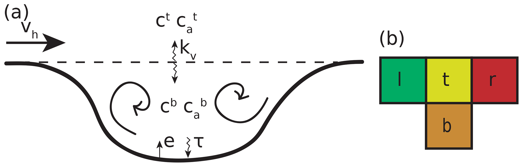
Figure 1(a) Schematic overview of the different processes influencing the average concentration cb and age concentration within an orographic basin. The processes include horizontal advection by the geostrophic wind (vh), vertical diffusion (kv), emission (e), and deposition (τ). (b) A highly simplified spatial discretization to solve Eqs. (1) and (2) for the model depicted in (a).
Finally, to graphically illustrate the remarks given above, Eqs. (1) and (2) are integrated numerically for an idealized basin cross section to compare the two contrary cases. The idealized 2-D simulation experiments use grid cells with a uniform spatial resolution of 5 m as well as terrain-following vertical coordinates to represent a pot-shaped depression in the domain center given by the terrain-height function:
The domain is periodic in the y direction. As for the meteorological initial conditions, a horizontally constant potential temperature profile is prescribed with 280 K at the surface and a vertical gradient of K m−1. Zero specific humidity is used. The initial wind speed along the x axis is u=5 m s−1, the same value is also continuously prescribed as the domain-top boundary condition for velocity. Using periodic boundary conditions in the x direction for meteorology, a boundary layer develops and a CAP builds up within the sheltered basin with progressing simulation time. Quasi-stationary conditions occur after 2 h of simulation time. Emission source S1 is placed near the basin floor at x=300 m and source S2 on the left basin rim at x=80 m. Both sources extend infinitely along lines in the periodic y direction and emit at a constant rate of 0.2 µg m−1 s−1.
Figure 2a, c, and e show the distribution of c, ca, and the mean particle age a for an emission source placed at the bottom of the basin. In this case, the recirculation effect of the emitted tracer is reflected both in c and ca, as both fields show a significant accumulation within the pot-shaped basin. In Fig. 2b the emission source itself is visible by a quite sharp maximum, which is not seen in Fig. 2d. The associated mean particle age a (Fig. 2f) shows a complementary distribution to c in the sense that the emission source and the surrounding volume are characterized by a minimum and lower-than-average values, respectively. This is a result of the diluting effects of freshly emitted particles with zero age. Next, Fig. 2b, d, and f show the second case, where the emission source is located on the plateau above the left sidewall. As the emissions are also allowed to vertically disperse into faster-moving layers of air, the concentration generally tends to decrease with increased downwind distance from the source. Some of the emissions entering the basin are trapped within the recirculation zone covering the lower half of the basin. As a result, the distribution of c within the basin is quite homogeneous (which reflects cb≈ct). In contrast to c, the distribution of ca (Fig. 2c) is fundamentally different, as the emission source is not directly visible, but instead the effect of the recirculating air within the basin is reflected by the accumulation of ca. Note also that in this case the distribution of ca and a has a quite similar appearance (as opposed to c and ca in case 1). More generally, of the set of the three depicted variables, only ca shows a consistent spatial pattern among the two contrary cases, as indeed the patterns in Fig. 2c and d appear to be quite similar. While the spatial distributions of c as well as a are dominated by the emissions, the spatial distributions of ca show an accentuation of the flow properties regarding the fact of that the direct effects of emissions are masked and the zones of recirculating or stagnant air are rendered visible by local maxima in ca. Put another way, it could be also argued that regions marked by high values of ca are especially prone to accumulation of air pollutants if additional emissions occur into that volume. A natural limitation of the proposed approach is clearly that ca still depends indirectly on the distribution of emissions. However, as seen in this simplified example, the overall spatial patterns can nevertheless be expected to be rather insensitive in this regard.
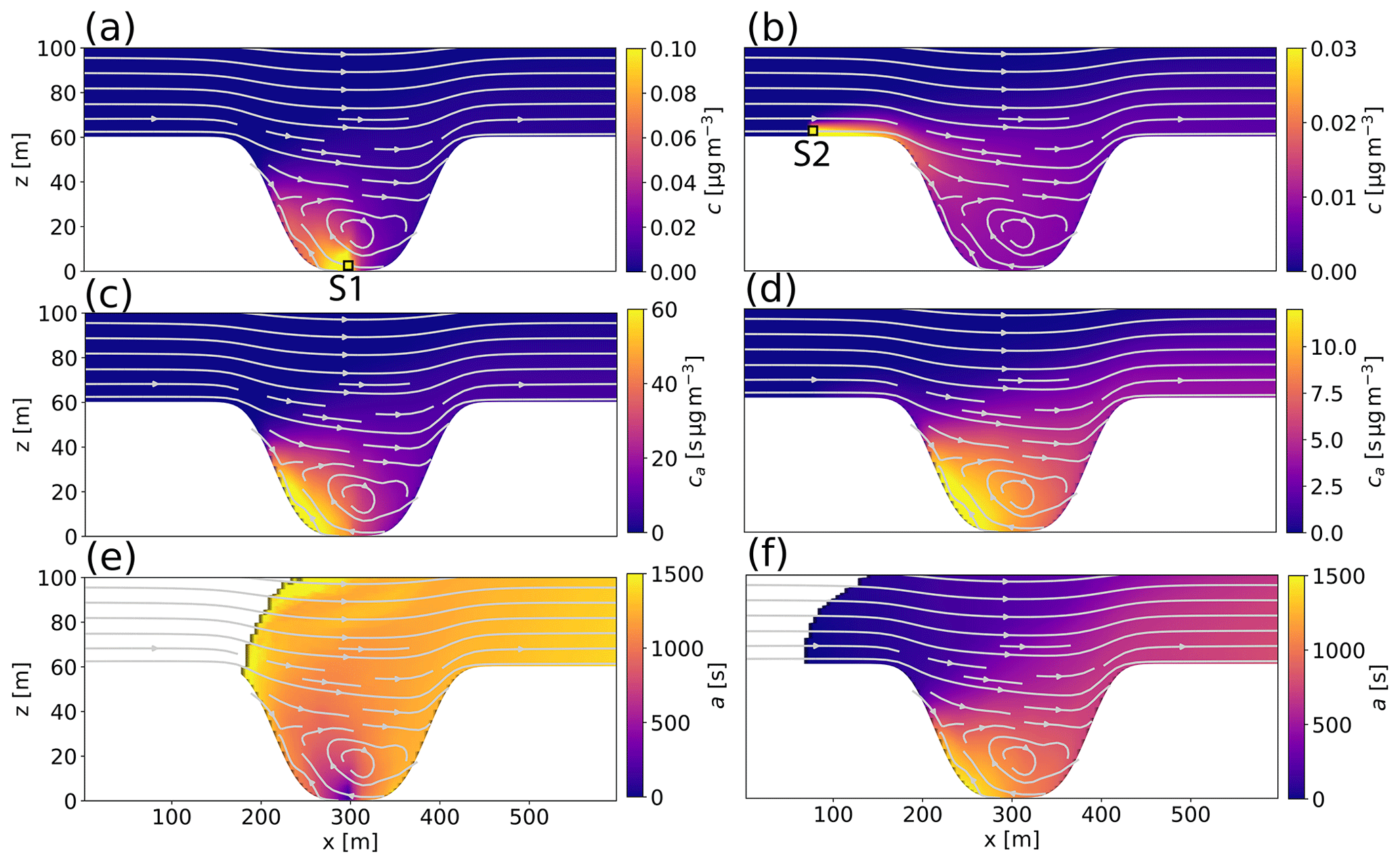
Figure 2Numerical solutions of the concentration field c (a, b), the age-concentration field ca (c, d), and the mean particle age field a (e, f) for idealized 2-D (periodic in the y direction) dispersion experiments. In experiment 1 (a, c, e), the emission source (red pixel, label “S1”) is located at the bottom of the pot-shaped depression. In experiment 2 (b, d, f), (label “S2”) it is located outside the depression near the left domain boundary.
2.2 Real-case simulation study
2.2.1 Model description
The urban large-eddy simulation model CAIRDIO is suitable for simulating emission, transport, and deposition of chemically inert air pollutants over complex topography at spatial resolutions ranging from the lower end of the mesoscale down to the microscale. Two different approaches are used to represent topography in the model. The surface orography, which excludes buildings, is represented using terrain-following coordinates, while the buildings themselves are physical obstacles represented by diffuse-obstacle boundaries (DOB) in the Cartesian framework. CAIRDIO solves the incompressible fluid-dynamics equations with the anelastic approximation and employs a simple TKE-based subgrid model of the Smagorinsky type (Deardorff, 1973) for unresolved turbulent motions. A detailed model description of CAIRDIO can be found in Weger et al. (2021) and Weger et al. (2022a). In the newest model version 2.1 used in this study, an improved multiple linear regression model to downscale surface temperature and surface specific humidity from mesoscale model output is used. More details on this downscaling scheme can be found in Appendix A1. In addition to the default transport equation (1) for air pollutants, Eq. (2) was implemented in CAIRDIO v2.1 to adapt the model to the required capabilities in the framework of this study. For the solution of the resulting time-discrete coupled system of equations, Eq. (1) is first advanced in time with a suitable explicit scheme. The arithmetic average of the old and new states of c is then used as the aging term in Eq. (2). The transport terms in both equations are discretized with a flux-limited linear advection scheme to provide positive solutions for c and ca. It must be noted, however, that linear correlations between c and ca and hence positivity of a are not guaranteed unless a more strict flux-limiting criterion is used (Deleersnijder et al., 2020).
2.2.2 Model setup
The simulation domain (labeled D4), to which CAIRDIO is applied, covers an area of roughly 29 km × 25 km with 60 m horizontal resolution (490 × 420 grid cells in the horizontal plane). The domain is centered around the city of Dresden and incorporates the entire cross section of the Elbe Valley section with its surrounding elevated planes (see Fig. 4 for an overview). The vertical grid encompasses 32 layers, with the first model layer following the surface orography, which is progressively smoothed out with increasing height. The uppermost model layer has a constant altitude of 1240 m above sea level. Vertical resolution near the ground is 5 m and near the domain top 120 m. Realistic BC emissions for industry, housing, and transport are primarily based on a gridded emission inventory (500 m × 500 m resolution) from the German Environmental Agency (UBA) valid for the year 2020. Industrial and housing emissions are further downscaled to the building sites. Within the city area of Dresden, UBA road transport emissions are substituted by spatially more accurate emissions from the Sächsisches Landesamt für Umwelt, Landwirtschaft und Geologie (LfULG). An overview of the resulting BC emission dataset is shown in Fig. S4. More details on the emissions and other input data used to describe surface orography, buildings, and land-use cover can be found in our previous modeling study (Weger et al., 2022a). Realistic meteorological and atmospheric composition boundary conditions with 180 s time resolution are provided with precursor simulations using the coupled weather prediction and air-chemistry transport model system COSMO-MUSCAT (Wolke et al., 2012). COSMO-MUSCAT is applied to a hierarchy of domains with spatial resolutions of 7, 2.8, 1.4, and 0.7 km using a one-way nesting approach (shown in Fig. 3). Domain D0, covering Germany and other parts of central Europe, is initialized and driven by 3-hourly re-analysis data of the operational weather prediction model ICON-EU run by the German Weather Service (Deutscher Wetterdienst, DWD). Initial and boundary conditions for the BC concentration are provided by a European-wide COSMO-MUSCAT simulation with 14 km resolution, which itself is driven by re-analysis data from the operational ICON global model, and air-chemistry data from the ECMWF IFS model (Copernicus Atmosphere Monitoring Service) (Flemming et al., 2015). For domain D3, the double-canyon effect parameterization DCEP (Schubert et al., 2012) is applied to simulate the effects of buildings and impervious ground surfaces on the mesoscale atmosphere. More technical details on the mesoscale simulation setups, the input datasets used, and the interpolation of model results from mesoscale domain D3 to the CAIRDIO domain D4 can also be found in Weger et al. (2022a).
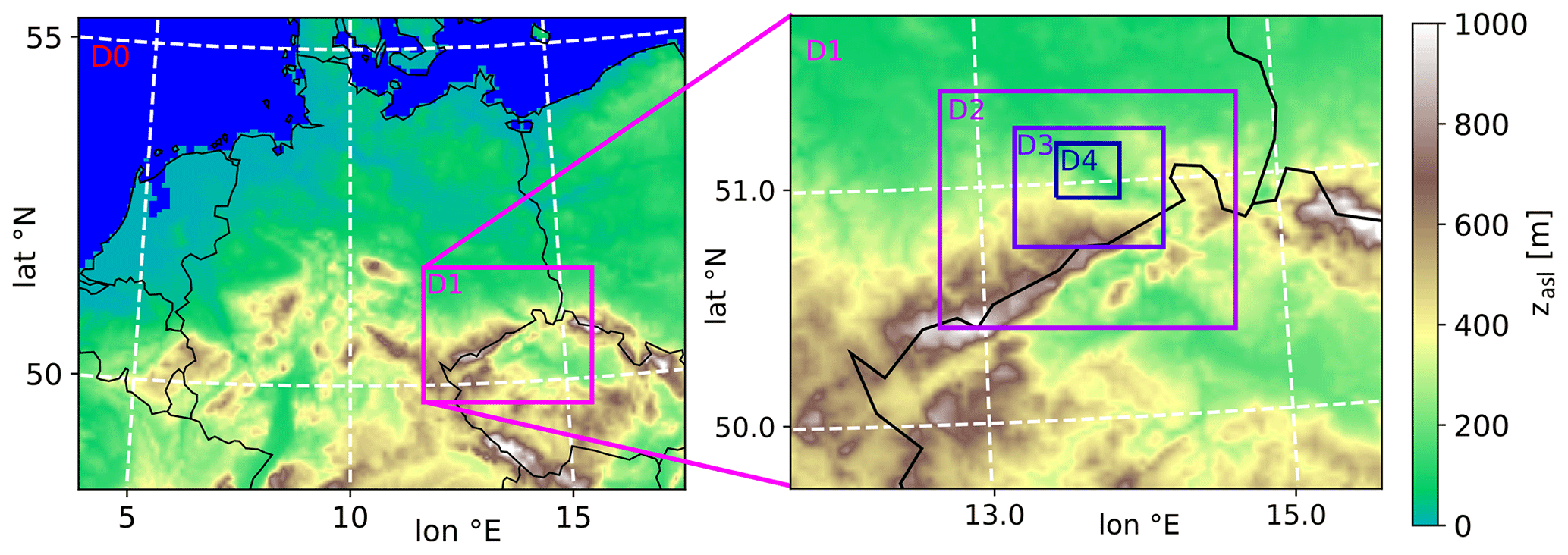
Figure 3Overview of the model nesting chain (indicated by colored boxes) used to downscale meteorology and air composition toward the city area of Dresden. The mesoscale domains D0, D1, D2, and D3 are simulated with COSMO-MUSCAT. The target urban gray-zone domain D4 is simulated with CAIRDIO; zasl refers to height above sea level.
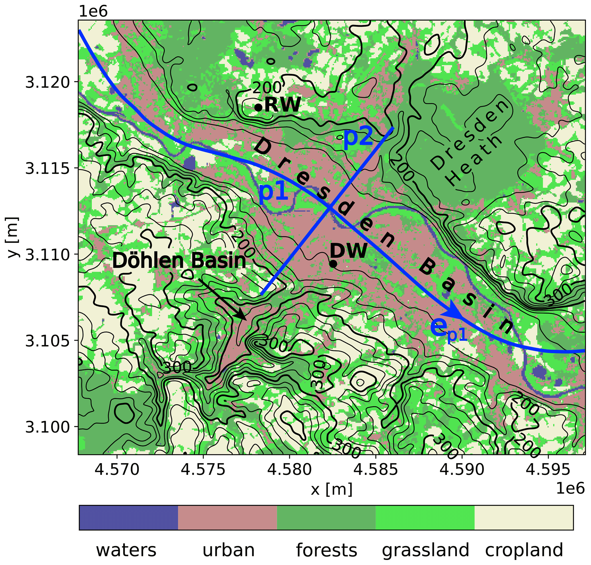
Figure 4Overview of simulation domain D4 simulated with CAIRDIO. The distribution of land use, smoothed surface orography by black contours with 25 m spacing, the position and label of the background air monitoring stations Dresden Winckelmannstr. (DW) and Dresden Radebeul (RW) (see Sect. S1 in the Supplement for a description of the sites) are shown by black dots and labels, and paths p1 and p2 followed to extract vertical profiles of model data are shown by blue lines and labels. ep1 is the local tangential unit vector to path p1. x and y coordinates of the map refer to the ETRS89-extended/LAEA Europe projection (EPSG:3035).
2.2.3 Dispersion experiments
CAIRDIO is applied to simulate the boundary-layer evolution, as well as to host multiple BC dispersion experiments for a total time span of 24 d. This duration encompasses two separate simulation periods, each one 12 d long. Period T1 is in late winter 2021 from 27 February, 00:00 UTC to 11 March, 00:00 UTC, and period T2 in early summer 2021 from 31 May, 00:00 UTC to 12 June, 00:00 UTC. As for the BC transport simulation part, a first dispersion experiment is performed that uses the emissions described in Sect. 2.2.2 and lateral boundary conditions of the precursor air quality simulation D3 with COSMO-MUSCAT. This experiment (labeled “BC-full”) has the purpose of including a model validation in our study by comparison of model results with BC measurements from operational air-monitoring stations. The results of this validation are presented in Sect. S1. The actual dispersion experiment relevant to the study of orographic effects uses the same BC emissions as experiment BC-full, but solves the system of Eqs. (1)–(2). In contrast to BC-full, no lateral boundary conditions are prescribed for the mass and age concentration (i.e., homogeneous zero Dirichlet conditions are used). This approach is equivalent to a tagging of the local emissions, for which reason this simulation run is labeled “BC-tag”. Note that the regional background contribution, which is missing in BC-tag, is expected to be spatially homogeneous anyway, and only temporally variable at the local scale. In a third and final experiment, the realistic emissions are replaced by horizontally homogeneous emissions with a constant in space and time emission rate per horizontal unit area, while all other model settings apply to experiment BC-tag. This experiment is labeled “BC-hom” and used to test the sensitivity of the age-concentration distribution to the emissions.
3.1 Meteorological conditions
3.1.1 Period T1: 27 February–10 March 2021
The synoptic weather situation during the first simulation period T1 ranging from 27 February 2021, 00:00 UTC to 11 March 2021, 00:00 UTC was dominated by a blocking high-pressure system over northwestern Europe, which persisted from the beginning of the simulation period until 9 March and also temporarily expanded over central and southeastern Europe, from 28 February to 3 March (see Fig. 5a). Westward shifts of the high over the British Isles prompted the intrusion of cold continental air mass over eastern and central Europe, with a significant event during 4–5 March (Fig. 5b) and a less pronounced one also on 8 March. Near the end of the simulation period, the blocking pattern over Europe resolved as northwestern Europe was increasingly affected by an Icelandic low (not shown). The implications of the synoptic-scale meteorological situation on the temporal evolution of the boundary-layer structure in the Dresden Basin are shown in Fig. 6a–c. Figure 6a shows the prevailing horizontal wind above the basin's average sidewall height (>300 m), while Fig. 6b shows the along-valley wind speed within the basin. The first 2 simulation days were still influenced by northwesterly winds (generally below 7 m s−1), which translated to an up-valley (west-northwest) wind within the basin. The up-valley wind was the strongest during daytime (up to 6 m s−1), presumably as a result of convectively enhanced vertical momentum transport (see Fig. 6c for the stratification and boundary-layer height). As the high pressure expanded over central Europe over the next consecutive days during 2–3 March, the prevailing winds shifted to the southeast and further weakened to below 4 m s−1. This led to the formation of down-valley (east-southeasterly) winds, which this time were the strongest during nighttime. In particular, a nocturnal low-level jet can be identified by distinct wind maxima in about 100 m height (wind speed up to 5 m s−1). The jet is presumably a result of CAP formation within the Dresden Basin (also evidenced by the elevated maxima in the vertical gradient of Θv) and the resulting vertical decoupling of the basin atmosphere and the free troposphere aloft. Note that this decoupling is also evident by the picking-up westerly winds after 3 March, 00:00 UTC, which do not mix down into the basin atmosphere until after sunrise. During the course of 3 March, westerly winds further increased to up to 10 m s−1 and eventually turned to the north with the aforementioned intrusion of cold air on 4 March. The quite strong winds prevented the nocturnal stabilization of the boundary layer so that up-valley winds consistently prevailed from 4 March 00:00 UTC to 6 March 00:00 UTC. Thereafter, the wind speed temporarily decreased to allow for intermittent nocturnal decoupling of the basin atmosphere (e.g., in the early morning of 6 June and on 7 June around 00:00 UTC). Northwesterly winds briefly increased again during the night from 8 to 9 March. Thereafter, a period characterized by weak southeasterly winds aloft and down-valley winds within the basin with an apparent nocturnal jet resumed until near the end of the simulation period.
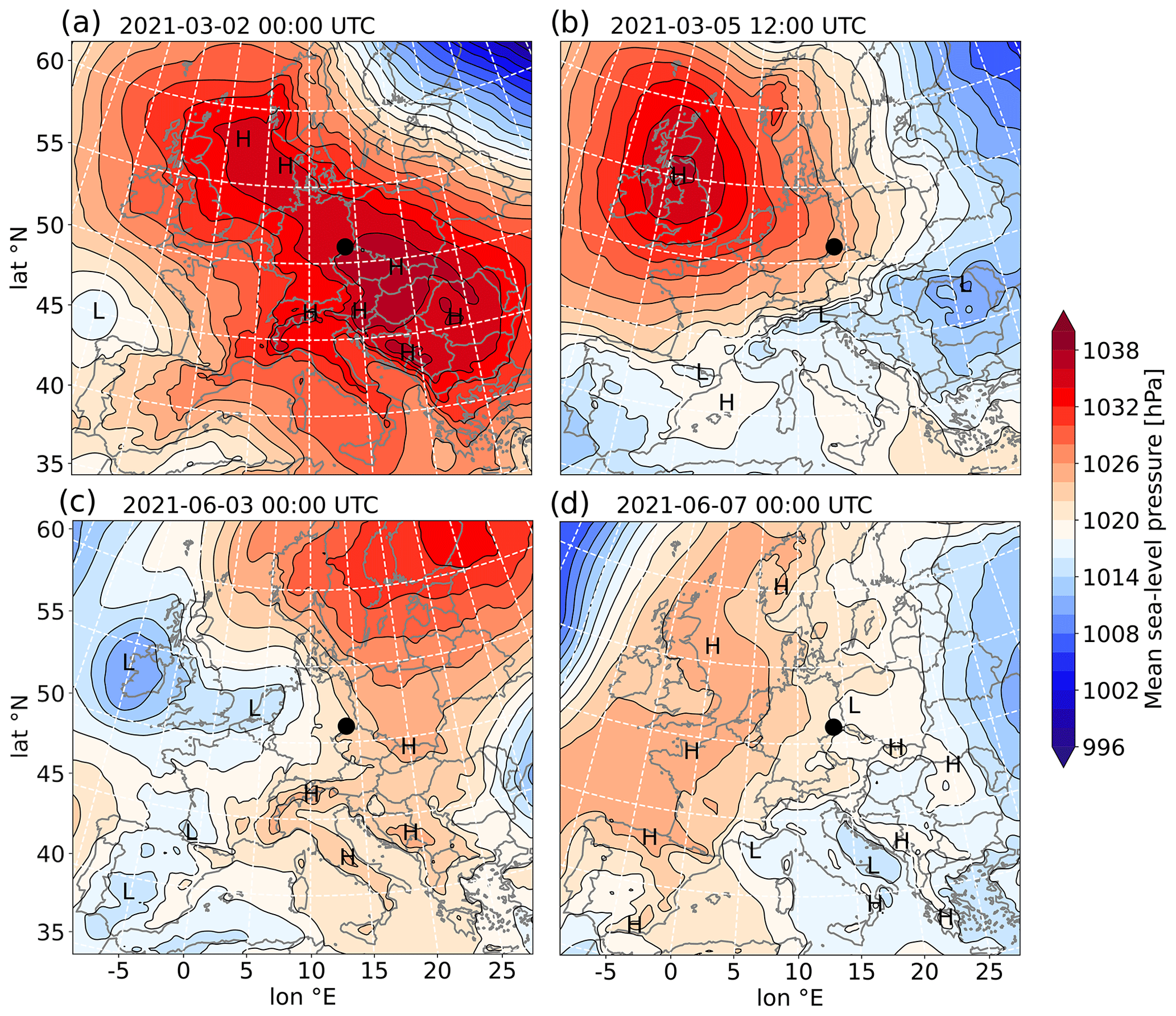
Figure 5Synoptic-scale maps of mean sea level pressure over parts of Europe as considered representative for the prevailing weather patterns during simulation period T1 (a, b) and T2 (c, d), respectively. The maps are based on re-analysis data of the global forecast model ICON (13 km) of the DWD. The black circle marks the geographical position of the city of Dresden.
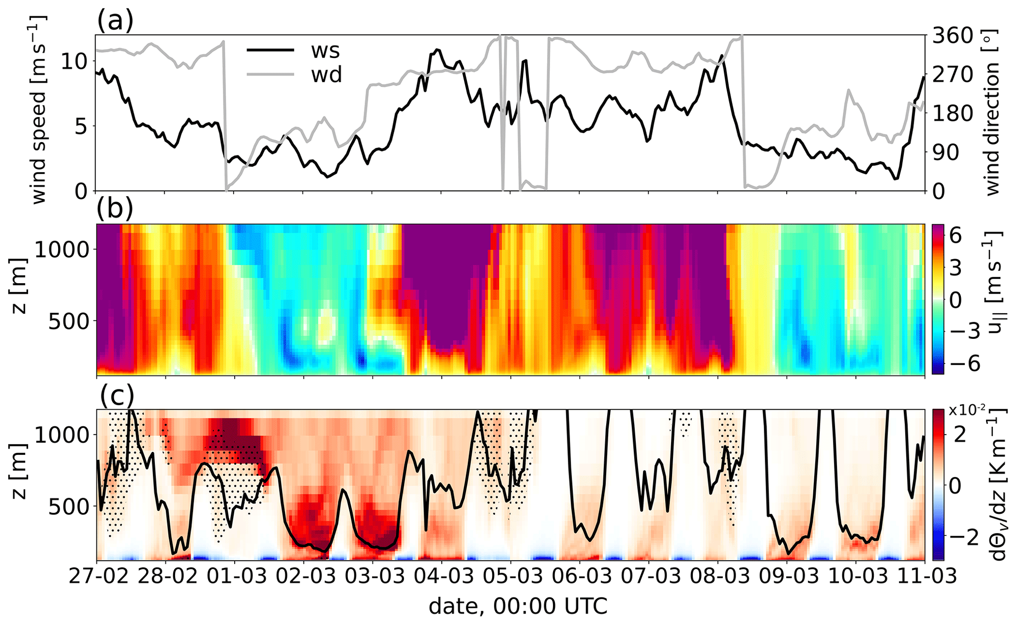
Figure 6Model data averaged along path p1 (shown in Fig. 4) vs. time for the late winter simulation period T1: In (a) the wind speed (black line) and wind direction (gray line) are averaged for the height range from the Dresden Basin average side-wall height (300 m) to the domain top. Panel (b) shows the vertical profile of the along-valley wind speed , which is defined by the dot product of the wind vector u with the local tangential unit vector to p1 ep1 (see Fig. 4) (). Positive values are related to up-valley winds. Panel (c) shows the vertical gradient of virtual potential temperature (color plot), the boundary-layer height estimated from the bulk Richardson number (black line), and cloudiness (dotted pattern).
3.1.2 Period T2: 31 May–11 June 2021
Similar to simulation period T1, a blocking pattern over Europe also characterized simulation period T2. The core of high surface pressure was, however, this time located over Scandinavia and western Siberia instead of northwestern Europe. This pattern allowed Atlantic disturbances to protrude more easily toward western and central Europe during the first half of the simulation period (Fig. 5c). During 4–5 June, an eastward moving cut-off low was associated with the development of locally intense thunderstorms over parts of France, Benelux, and Germany (not shown). The easternmost regions of Germany were, however, only marginally affected by this activity. On 6 June, high pressure built back over western Europe to form an extensive high-pressure ridge stretching from southwestern Europe all the way to Scandinavia (Fig. 5d). Central Europe remained under the influence of this high-pressure ridge until the end of the simulation period. Figure 7a–c show again the evolution of the planetary boundary layer structure in the Dresden Basin during this time period. During the first 2 simulation days, generally low-wind conditions with weak along-valley winds prevailed (below 5 m s−1). During the nighttime, the basin atmosphere became stably stratified and a ground-based inversion layer (seen by the large Θv-gradient near the surface in Fig. 7c) formed due to weak-to-absent along-valley winds. On 2 June, southeasterly winds ahead of an approaching trough increased to up to 8 m s−1. As a result, also the wind direction within the basin shifted and a significant down-valley wind developed. In fact, the wind maxima between 200 and 300 m height (up to 8 m s−1) can be associated again with the nocturnal low-level jet, which also coincides with the elevated maxima in the Θv gradient (Fig. 7c). Note, however, that despite the similarities with days 2–3 March of period T1, the thermal stratification is less stably stratified this time (cf. Fig. 6a–c). This is arguably due to a cyclonic influence over Germany at that time (Fig. 5c). As a weakening low moved eastward across France and southern Germany over the following 2 d during 4–5 June, the southeasterly winds diminished and the along-valley winds shifted to a pattern of weak up-valley winds during daytime and weak down-valley winds during nighttime. From 7 June on, the area was situated at the eastern flank of the aforementioned high-pressure ridge to the northwest with the wind direction shifting from northwesterly to northeasterly winds. Close to the surface, the winds turned more to the west from the effect of surface friction, with the winds in the Dresden Basin blowing in the up-valley direction for most of the time.
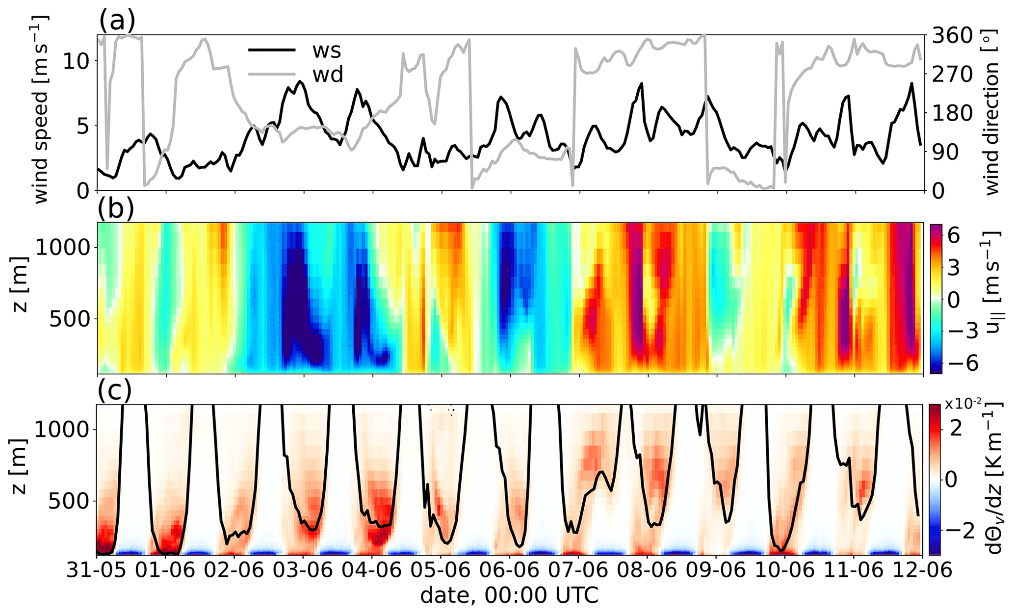
Figure 7Model data averaged along path p1 (shown in Fig. 4) vs. time for the early summer simulation period T2: In (a) the wind speed (black line) and wind direction (gray line) are averaged for the height range from the Dresden Basin average side-wall height (300 m) to the domain top. Panel (b) shows the vertical profile of the along-valley wind speed . Panel (c) shows the vertical gradient of virtual potential temperature (color plot), the boundary-layer height estimated from the bulk Richardson number (black line), and cloudiness (dotted pattern).
3.2 Temporal mean BC dispersion patterns
For an initial overview of the dispersion experiments, the temporal mean horizontal distributions of the BC concentration within the first model layer are discussed. In Fig. 8 respective patterns are shown for experiments BC-tag and BC-hom for the late winter period T1 and the early summer period T2, respectively. The patterns of experiment BC-full are not shown, as they differ only by a spatially near-uniform background offset of 0.28 µg m−3 for period T1 and 0.23 µg m−3 for period T2 from BC-tag. Firstly, it can be noted that the concentration distributions of experiment BC-tag (Fig. 8a, c) are strongly dominated by the traffic emissions, especially from highway A4, which crosses the Dresden Basin in a northeasterly direction, but also from other major roads within the city area of Dresden. Aside from these prominent line features, which exceed a concentration of 1 µg m−3, accumulations of BC with a spatially more uniform distribution can be discerned within the Dresden Basin. This is especially the case during the generally more stable period T1 (Fig. 8a) when average concentrations amount to at least 0.3 µg m−3. In this regard, the sharp gradient along the northern fringe of the basin is also striking, which is rendered visible by the underlaid terrain shading. The average concentration level during period T1 is higher than during period T2 (0.18 µg m−3 vs. 0.10 µg m−3). This difference cannot be explained by a different emission rate, which on average is 1.48 kg h−1 over the entire domain D4 volume during period T1 and 1.35 kg h−1 during period T2. We also briefly discuss the BC dispersion patterns of experiment BC-hom at this point, which are further used in Sect. 3.3. In contrast to BC-tag, in experiment BC-hom, the BC distributions are solely determined by meteorology. As a result of the spatially homogeneous emissions, the bulk of BC mass is distributed over a wider area compared to experiment BC-tag, where it is more focused over the city area. The effect of surface orography is very eminent, as higher-than-average concentrations are generally found within topographic depressions, like the Dresden Basin, which sticks out during both simulation periods. During period T1 (Fig. 8b), a marked variability within the Dresden Basin is also apparent, as prominent maxima of roughly 0.3 µg m−3 are present to the north and south of the Dresden city area and over the southern basin sidewall. Within the remaining parts of the Dresden Basin, concentrations average out at 0.15 µg m−3. Aside from the Dresden Basin, high concentrations are also reached within the southern tributary valleys. The most striking feature here is the Döhlen Basin containing the city of Freital, wherein the domain-maximum concentration of about 0.5 µg m−3 is reached. For period T2 (Fig. 8d), the focus of BC concentration maxima is shifted from the southern tributary valleys to some shallow depressions north of the Dresden Basin, where concentrations reach up to 0.2 µg m−3 (e.g., over parts of the Dresden Heath, a large forest area to the northeast of the city).
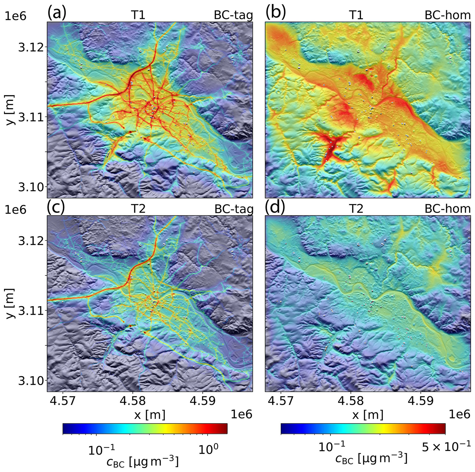
Figure 8Temporal mean BC concentration cBC patterns of dispersion experiments BC-tag (a, c) and BC-hom (b, d). The concentration in BC-hom is rescaled such that the area-sum equals that of experiment BC-tag. Note that different color scales are used for BC-tag and BC-hom. The patterns in (a, b) refer to the simulation period T1, the patterns in (c, d) to period T2.
3.3 Age-concentration modeling: proof of concept
While the BC concentration patterns of experiment BC-tag provide an overview of the simulated air pollution situation and also show the contrast between the late winter and early summer period, it is not yet conclusive which orographic features act as secondary pollution sources under the most realistic scenario studied. On the one hand, the use of realistic emission data results in intrinsic spatial inhomogeneities that are superimposed on the spatial features induced by orography, making it potentially difficult to disentangle both effects. On the other hand, the simulation using spatially homogeneous emissions provides only an overview of potential orographic hot spots, but from this perspective, it cannot be concluded whether an orographic region with significant air pollutant accumulations is also relevant when imposing a more realistic emission scenario. At this point, the age-concentration concept, which was introduced in Sect. 2.1.2 in the framework of air-pollutant dispersion modeling, may provide a more conclusive picture in this regard. Similar to Fig. 8, Fig. 9 shows the temporal mean BC dispersion patterns for experiments BC-tag and BC-hom, but now for the age concentration ca,BC instead of the mass concentration cBC. As already pointed out, the direct effects of the emissions are masked in the age-concentration fields, and the regions that are characterized by stagnant or recirculating air mass are highlighted by high values of ca,BC. The ca,BC patterns of the dispersion experiment BC-tag show that the entire modeled section of the Dresden Basin is very well marked off by elevated values compared to the adjacent higher-elevated planes, especially along the northern fringes of the basin. The intra-basin distributions of ca,BC show some marked differences between simulation periods T1 and T2. During period T1 (Fig. 9a), the focus is more on parts of the city area ( s µg m−3) but even more so over the southwestern sidewalls of the basin ( s µg m−3) and the Döhlen side basin, wherein ca,BC exceeds 2.5×10³ s µg m−3. During simulation period T2 (Fig. 9c), ca,BC is much more symmetrically distributed with generally lower values compared to period T2. The highest values occur over the city center ( s µg m−3). Note that the lower values toward the domain borders are likely related to the zero-Dirichlet boundary conditions prescribed for cBC and ca,BC there. Comparing the patterns of experiment BC-tag with experiment BC-hom (Fig. 9b, d) shows that the most important orographic hot spots identified by ca,BC in BC-tag are also present in BC-hom. For example, quite similar values of ca,BC are reached for the Döhlen Basin in both experiments, and ca,BC is also elevated over the southwestern sidewalls of the Dresden Basin in experiment BC-hom during period T1. Over the central parts of the Dresden Basin, where the city center is located, ca,BC is lower by about 20 % in experiment BC-hom compared to BC-tag. This difference stems from the much more concentrated emissions over the urban areas in BC-tag compared to BC-hom. On the other hand, there are also ca,BC accumulations apparent over some areas north of the Dresden Basin in Fig. 9d for experiment BC-hom and period T2, which are not seen in Fig. 9c. As already pointed out in the discussion of respective cBC patterns, these potential areas are not active in the realistic-emission setup, as emissions are in fact only sparsely distributed in these areas, e.g., the Dresden Heath. Comparing Fig. 8b with Fig. 9b and also Fig. 8d with Fig. 9d reveals that many of the local maxima seen in cBC are even better defined in ca,BC. In this regard, the stationary solutions of and of the simplified model derived in Sect. 2.1.2 can be recalled, which describe the potentiated spatial contrast in the field of ca,BC compared to cBC. Finally, the comparison between Fig. 9a and b, as well as Fig. 9c and d, supports the conjecture that ca,BC is rather insensitive to the emission distribution. In effect, from the aforementioned similarities, it can be argued that the age concentration is a suitable metric for identifying orography-related pollution hot spots, especially since it enables the incorporation of realistic emissions. Finally, for the sake of completeness, the mean particle age aBC of experiment BC-tag is shown in Fig. S5. Compared to the distribution of cBC, the emissions are now visible by lower-than-average values. Conversely, the highest values of aBC typically occur in areas with low emissions, e.g., the Dresden Heath, where aBC exceeds 1 h. Causally, the effect of the trees is a deceleration of the horizontal wind speed and in turn an increased residence time for horizontally advected BC. However, the potential for air pollution trapping only becomes relevant if significant emissions occur upwind of the area. In comparison to the Dresden Heath, this is the case for the Döhlen Basin, where over the side slopes similar high values of aBC occur during period T1. Note that in general, aBC is significantly higher over the planes to the south of the Elbe River Basin during period T1 compared to period T2, which is indicative of the different meteorological conditions prevailing on average between both simulation periods.
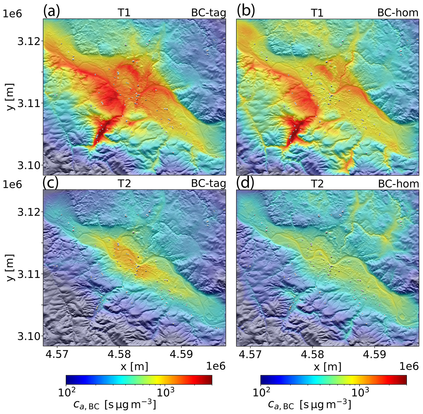
Figure 9Temporal mean BC age-concentration ca,BC patterns of dispersion experiments BC-tag (a, c) and BC-hom (b, d). The patterns in (a, b) refer to the simulation period T1, the patterns in (c, d) to period T2.
3.4 Characteristic meteorological and BC dispersion patterns
After describing the temporal mean BC mass and age-concentration distributions, it remains open to explain the temporal variability of BC transport in the Dresden Basin and how it is affected by specific meteorological situations, which change from day to day, but also between daytime and nighttime. By associating the key dominant meteorological patterns (in terms of temporal variance represented) with characteristic BC transport patterns, we can better understand under which meteorological conditions air pollution trapping is most significant. In addition, we can finally conclude whether the temporal mean BC distributions are predominantly influenced by a specific meteorological pattern associated with orographic wind systems, which can already be conjectured from the orographic features in Fig. 9. An empirical orthogonal function (EOF) (also referred to as “principal component”, PC) analysis is used to find the most important near-surface wind field patterns during the simulation periods. It can be noted that the EOF analysis is especially appropriate for mountain and valley wind systems, because the temporal variability of these systems can be well characterized by only one or two dominant modes (e.g., the wind direction up or down the valley often already describes a large part of the temporal variability). The EOF methodology applied on observational wind data is described in Ludwig et al. (2004). Here, we apply it on the simulated wind field within the first model layer of domain D4. Instead of resorting to standard non-rotated EOF analysis, however, we use rotated EOF analysis (varimax rotation), as it can better capture the physically relevant modes (Lian and Chen, 2012).
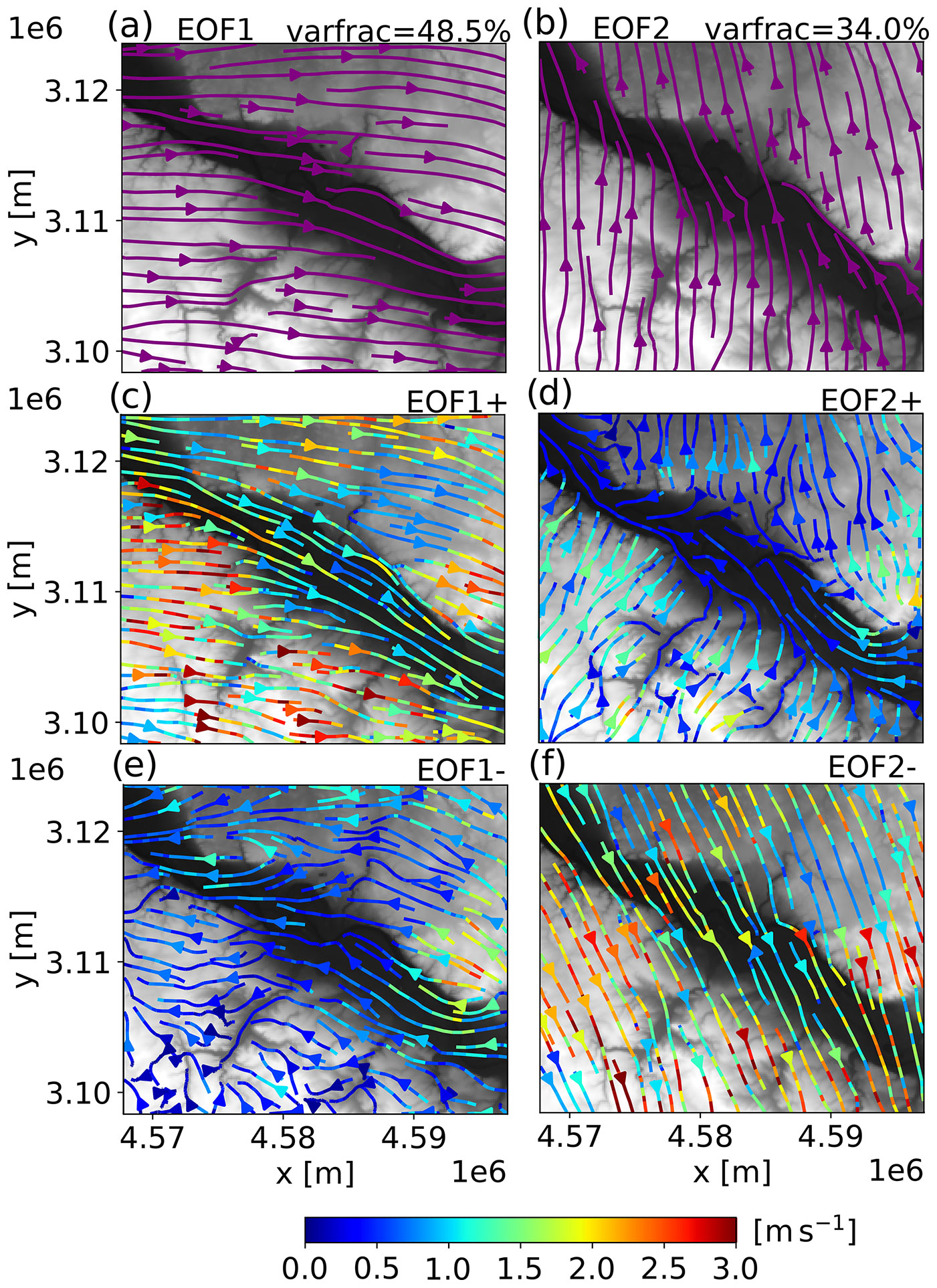
Figure 10Streamline pattern of the first (a) and second (b) rotated EOF. fvar indicates the percentage of the total variance described by the corresponding EOF. Panels (c) and (e) show the average reconstructed near-surface wind field for a positive and negative amplitude (computed with Eq. 18 over period T1 and T2) of the first EOF, while (d) and (f) show the same information for the second EOF. The color bar indicates the horizontal wind speed of the reconstructed wind field patterns in (c)–(f).
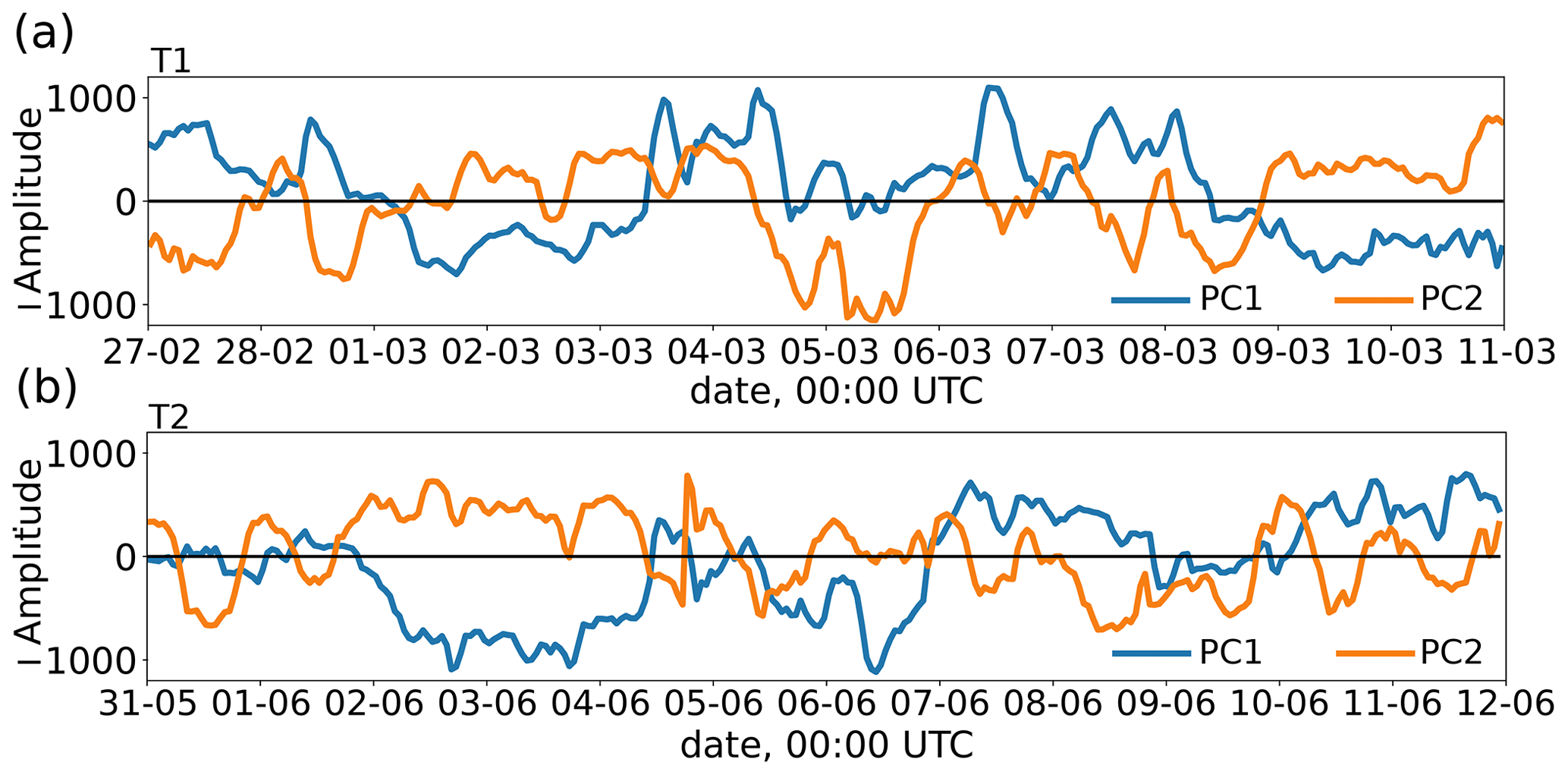
Figure 11Principal component (PC) time series PC1 and PC2 associated with the rotated EOF1 and EOF2 for simulation period T1 (a) and T2 (b), respectively.
The first two rotated EOF modes of the near-surface wind field of domain D4 computed for the combined simulation period T1 and T2 are shown in Fig. 10a and b. It is noteworthy that the first two modes already include 82.5 % of the total temporal variance of the data. EOF1 obviously describes the variability of westerly and easterly winds while EOF2 describes the variability in the north–south direction. Hence, the first two EOFs can be considered to form a base for the variability of the large-scale wind and the consecutive EOFs are more related to noisy and insignificant small-scale variability (fvar=1.2 % for EOF3, not shown). The PC time series corresponding to the EOFs, which essentially are the amplitudes of the modes, are shown in Fig. 11. We can use the PC series in temporal weighting functions to derive the prevailing wind patterns for a negative and positive amplitude of the first two EOFs, respectively:
where n is the temporal sample size. In doing so, we get four near-surface wind patterns in total, which are shown in Fig. 10c–f. A positive amplitude of the first EOF (EOF1+) results in west-northwesterly winds over the elevated planes (up to 3 m s−1) and an up-valley wind within the Dresden Basin. This pattern is associated with a generally weaker boundary-layer stratification and greater nocturnal mixed-layer heights (cf. Fig. 11 with Figs. 7b and 8b). Days on which this pattern prevailed are 27 and 28 February as well as 4, 6, 7, and 8 March during period T1 (Fig. 11a). The second half of simulation period T2 was also often affected by this pattern (Fig. 11b). For the contrary case of EOF1− (negative amplitude), the prevailing wind direction is from the east-southeast with peak winds of 2 m s−1 over the highest planes. This case also corresponds to a more stable boundary-layer stratification and the occurrence of the nocturnal low-level jet. As in both cases, EOF1+ and EOF1−, the prevailing wind direction (either from the northwest or the southeast) is relatively well aligned with the orientation of the basin, no large differences in the wind direction between the basin and planes occur. This is different for the case of EOF2+ (Fig. 10d). Here, the prevailing wind direction is from the south-southwest over the planes south of the Dresden Basin and slightly rotated to the south-southeast over the northern planes. The weak down-valley wind (mostly below 1 m s−1) within the Dresden Basin is nearly perpendicular to the prevailing wind direction aloft, suggesting a very stable boundary layer stratification and a resulting vertical decoupling of the basin-interior air flow. From Fig. 11a and b it can be seen that this pattern was often present during the nighttime, e.g., on 2, 3, and 4 March during period T1. Occasionally, it overlapped also with the EOF1− pattern, e.g., from 2 to 4 June during period T2. The fourth and final pattern (Fig. 10f) refers to the case of EOF2−. This case is associated with stronger northwesterly winds (up to 2.5 m s−1) and only a small contrast in both wind speed and direction between the Dresden Basin and the adjacent elevated planes. In fact, the streamlines run mostly straight across the domain with little apparent influence from the underlying topography, which is indicative of a significant turbulent boundary layer being present. This pattern was most relevant during the cold-air intrusion on 5 March (Fig. 11a).
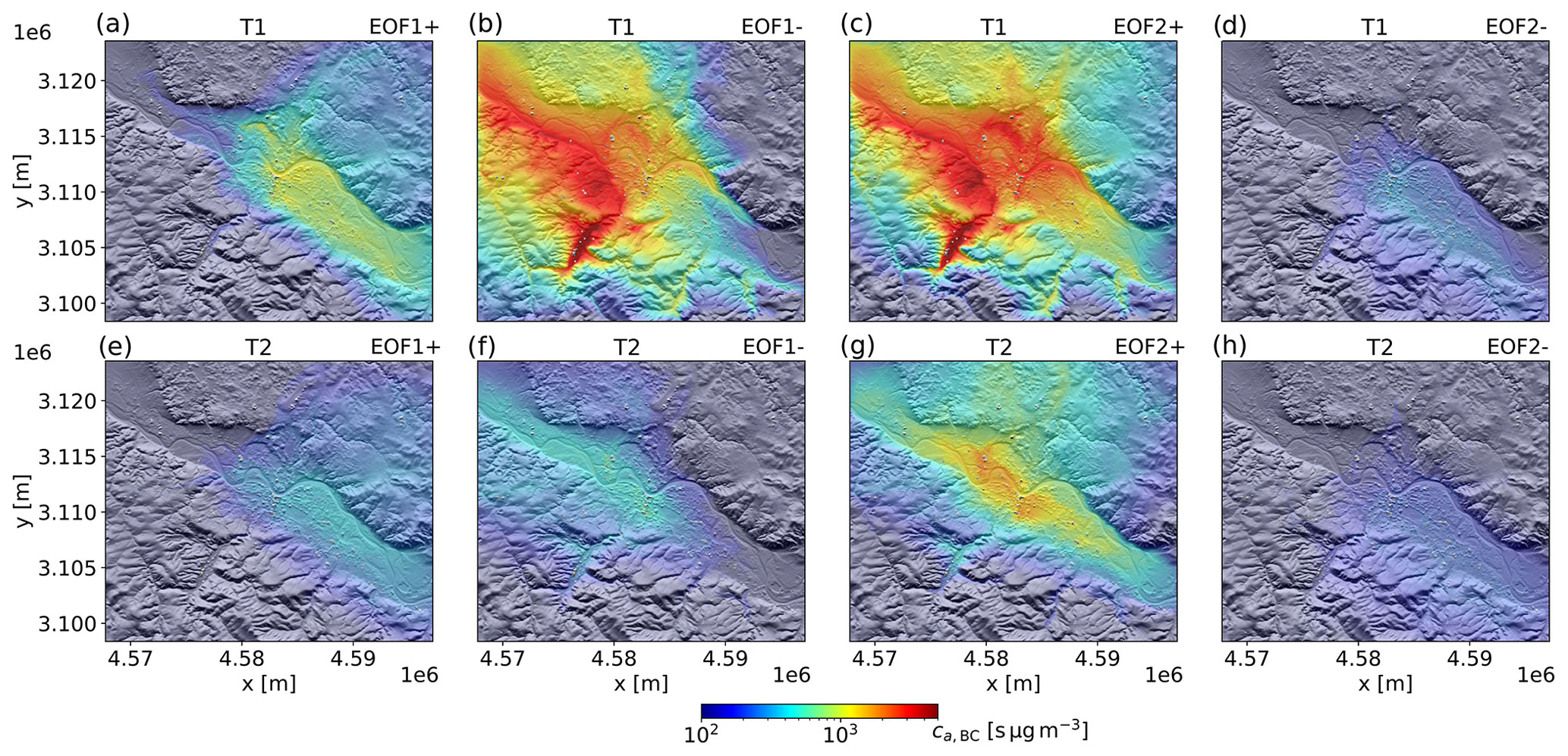
Figure 12Patterns of the BC age concentration within the first model layer computed with Eq. (18) for a positive and negative amplitude of the first (a, b, e, f) and second EOF (c, d, g, h), respectively. The patterns in (a–d) refer to the late winter period T1, and the patterns in (e–h) to the early summer period T2.
We can now derive the near-surface age-concentration patterns of BC associated with the wind field patterns in Fig. 10c–f using Eq. (18) again. Note that we can replace uh in Eq. (18) by any other model output variable, in our specific case by ca,BC of the simulation run BC-tag. In contrast to the wind field patterns, the two simulation periods are considered separately here, because it turned out that there are much more significant differences in the BC dispersion patterns between periods T1 and T2 compared to the differences in the wind field patterns. The resulting ca,BC patterns are shown in Fig. 12. As can be seen, the different EOF wind field patterns correspond to different magnitudes in BC age concentrations within the Dresden Basin. For example, cases EOF1− (Fig. 12b) and EOF2+ (Fig. 12c) show the highest age concentrations during period T1. These two cases are also the only cases associated with significant ca,BC accumulations within the Döhlen Basin ( s µg m−3). During simulation period T2, only case EOF2+ (Fig. 12g) gives evidence of significant air pollution trapping within the Dresden Basin. This is in contrast to case EOF2−, which shows only very low average BC age concentrations during both simulation periods (Fig. 12d and h). To exclude that a variable emission rate has any significant influence on the observed differences, the weighted average emission rates for the four different EOF patterns are also computed and listed in Table 1. Accordingly, the emission rate differs only by not more than 3 % between cases EOF2+ and EOF2−. When comparing Fig. 12 with Fig. 8a and c, the EOF2+ patterns resemble the temporal mean patterns in Fig. 8a and c quite well. This suggests that stably stratified cases with vertically decoupled down-valley winds within the Dresden Basin have an important influence on the average BC distributions in the Dresden Basin (compare also the corresponding EOF2+ BC mass concentration patterns in Fig. S6a and c with Fig. 8a and c).
Table 1Temporal mean BC emission rates computed with Eq. (18) and integrated over the domain D4 volume for the different EOFs and simulation periods. Units are in kg h−1.
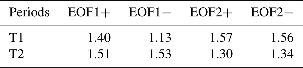
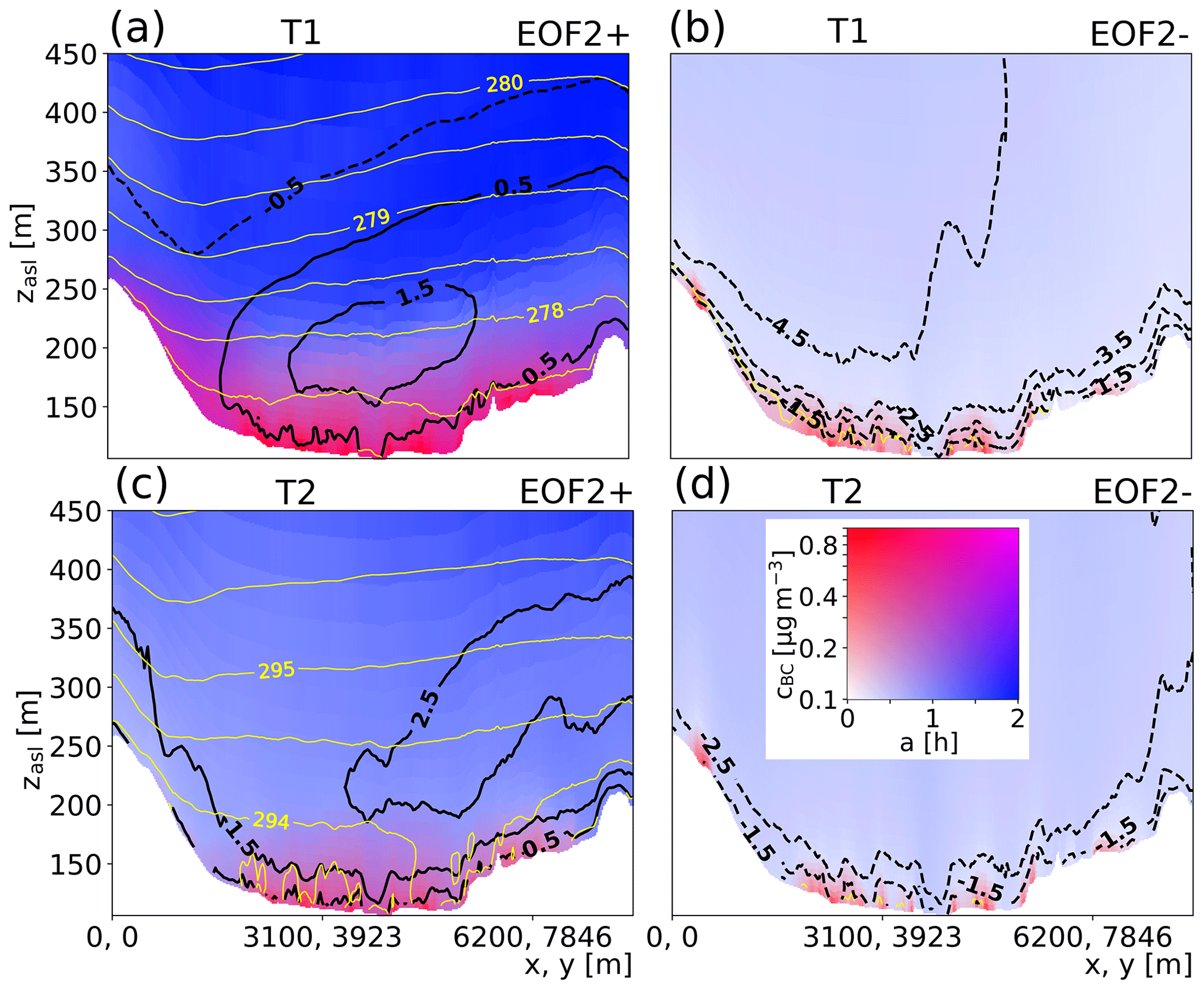
Figure 13Vertical distribution of black carbon mean particle age a (blue saturation, linear scale) and mass concentration cBC (red saturation, logarithmic scale) along the valley-perpendicular path p2 depicted in Fig. 4. Note that the vertical coordinate zasl refers to the height above sea level. The two different patterns for EOF2 are again computed with Eq. (18). In addition to the color plot, black contour lines show the magnitude and sign (dashed contours for negative sign) of the plane-perpendicular wind component (positive for the down-valley direction) and yellow contours show the virtual potential temperature (0.5 K spacing).
To confirm the assumption that the boundary-layer structure is a major factor in explaining the observed differences in the patterns of Fig. 12, Fig. 13 shows vertical cross sections of the BC concentration and mean particle age along path p2 (path shown in Fig. 4) for the two contrary cases of EOF2+ and EOF2−. In addition, yellow contour lines show the stratification, and black contour lines the along-valley wind. The saturated blue colors indicate a high average particle age (aBC>1.5 h), while pale blue colors indicate fresh aerosol. Similarly, saturated reds are associated with a high concentration cBC>0.5 µg m−3, and, finally, purple colors mark areas where both a high particle age and high concentrations overlap. Several observations can be made based thereon. Firstly, the EOF2+ case (Fig. 13a and c) is associated with a stably stratified boundary layer (high density of yellow contour lines) compared to case EOF2− (Fig. 13b and d), which shows a near-neutral stratification. This coincides with a positive plane-perpendicular or down-valley wind component (solid black contour lines) for case EOF2+ and up-valley winds (dashed black contour lines) for case EOF2−. For the EOF2+ case, thermal stratification is more pronounced during period T1 (Fig. 13a) compared to period T2 (Fig. 13c), and also the weak low-level jet core is better defined and confined to the basin interior during period T1 compared to T2. Secondly, a high mean particle age aBC in the upper model layers is correlated with a high mass concentration cBC near the bottom of the Dresden Basin and vice versa, which is irrespective of the simulation period. The case with the most stable stratification (EOF2+, T1) shows also the highest values in aBC and cBC near the surface among the cases considered. aBC reflects the large residence time of particles trapped within the Dresden Basin. Note in this regard that the decrease in aBC toward the ground is an effect of the urban emissions (cf. Fig. 2e of the idealized experiment in Sect. 2.1.2). Finally, the overlapping regions of high aBC and cBC correspond also to the areas where elevated values of ca,BC occur in the horizontal maps. In the case of EOF2+ during period T2, these areas are mainly confined to the central parts of the basin over the city area. During period T1, however, the same areas appear in a more saturated purple and extend also significantly over the sidewalls of the basin, especially over the southern sidewall.
The urban dispersion model CAIRDIO was applied on the Dresden Basin, a widened section of the Elbe Valley that contains the mid-sized city of Dresden, to investigate the influence of surface orography on the spatial distribution of BC as an important air pollutant. Two separate periods in late winter (T1) and early summer (T2) 2021, each 12 d long and characterized by predominantly calm weather conditions, were simulated. Realistic meteorological and air composition boundary conditions, as well as surface forcing, were generated with a nested hierarchy of mesoscale simulations with the coupled meteorological and air-chemistry model COSMO-MUSCAT. Two different emission scenarios were considered. In scenario BC-tag, a realistic BC emission dataset considering traffic, industrial, and residential emissions was used, which was also modulated in time to consider diurnal changes in activity. In a second scenario BC-hom, a spatially and temporally homogeneous BC emission rate was prescribed. Thus, in this dispersion experiment, the spatial distribution of BC was solely determined by the interaction of meteorology with topography. In addition to the simulation of emission, transport, and deposition of the mass concentration of BC, an additional similar transport equation for the BC age concentration was solved. As this transport equation does not directly depend on the emissions, it softens away the spatial inhomogeneities associated with the prescribed realistic emissions. Moreover, the age concentration typically reaches maximum values in areas characterized by stagnant or recirculating air, making it a useful metric with which to visualize air pollution trapping within orographic depressions during stable weather conditions.
As expected, the temporal mean distributions of BC mass concentrations were dominated by the line features associated with the traffic emissions in scenario BC-tag. Simulated domain-average BC mass concentrations were nearly twice as high during period T1 compared to period T2. This difference could be attributed to a generally more stably stratified boundary layer during period T1, although spatial differences related to surface orography remained inconclusive on the basis of the mass concentration of scenario BC-tag alone. By contrast, the mass and age concentrations of scenario BC-hom, as well as the age concentration of scenario BC-tag, showed a completely different picture that indeed highlighted orographic features and revealed also interesting differences between simulation period T1 and T2. During period T1, the Dresden Basin was marked off by higher values compared to the adjacent elevated planes. Maximum values were reached over the southwestern side slopes of the Dresden Basin, with the southern tributary Döhlen Basin appearing as the most prominent hot spot. During period T2, only the urban area within the central section of the Dresden Basin and some areas north of the Elbe Valley showed markedly elevated mass and age concentrations of BC. The main difference between the mass and age concentration of run BC-hom was that the age-concentration field provided an even better differentiation of air pollution trapping zones. This result can be explained by the simplified stationary solutions of the two respective transport equations. The similarities in the spatial age-concentration distributions between scenarios BC-tag and BC-hom prove the robustness of the orographic flow information included in the property of the age concentration, as it is not very sensitive to the spatial distribution of emissions. Nevertheless, scenario BC-hom showed false indications over some areas where in reality no air pollutant emissions occur. The age concentration can therefore be considered a more appropriate metric that reflects the accumulations from a realistic distribution of air pollutant sources.
As a second result of the study, the most prevalent flow regimes during the two simulated periods were identified. Therefore, a statistical EOF analysis was carried out and the resulting patterns were further characterized based on their influence on local air pollution exposure. The first two most important EOFs essentially represented two contrasting flow regimes: the first flow regime could be characterized by a northwesterly prevailing wind direction and a stratification close to neutral. By contrast, a southeasterly wind direction with generally weaker winds was associated with a much more stable boundary-layer stratification. This resulted in the establishment of local orographic wind systems, such as down-valley winds within the Elbe Valley. Only for this second flow regime, a pronounced accumulation of air pollution within the Dresden Basin and its tributaries occurred, which also dominated the temporal mean BC mass and age-concentration distributions.
This study provided a mainly phenomenological description of air pollution trapping within the Dresden Basin. An in-depth analysis of the physical forcing mechanisms behind the observed spatial patterns was beyond the scope of this paper. This, however, will be addressed in future work using even higher-resolved domains targeting interesting sub-areas revealed by this study, e.g., the Döhlen Basin.
A1 Improved diagnostic interpolation of surface variables
CAIRDIO depends on external surface fields for potential temperature ΘS, specific humidity qv,S, and pressure pS. While the former two fields are required in the computation of the surface fluxes for heat and moisture, pS provides the lower boundary condition in the derivation of a hydrostatically balanced reference atmosphere used in the anelastic approximation of the fluid-dynamic equations, and the cloud-saturation and radiative transfer schemes. In our former version of CAIRDIO (v2.0), the surface fields were obtained by a diagnostic downscaling of respective prognostic data from the hosting COSMO simulation (Weger et al., 2022a). The downscaling consisted of fitting the COSMO data into a linear regression model, which was based on land use as the only predictor. This approach proved to be computationally cheap and feasible, provided that surface orography was mostly flat. In the current model version v2.1 used in the framework of this study, the approach was extended to a more sophisticated multiple linear regression model to address this limitation. Land use is distinguished into five independent classes, namely, forests, grassland, waters, bare soil, and urban areas. A spatially varying temperature field of urban (impervious) surfaces is, however, already provided by the urban parameterization DCEP in COSMO and is simply interpolated using bilinear interpolation. Note that this particular approach is not followed for qv,S and pS, where the urban surfaces are included in the regression model. Additionally to land cover, predictors in the revised scheme now include surface elevation hS, surface normal orientation expressed by azimuth and elevation angles (ϕS, ψS), cloud attenuation ηcl, precipitation rate pr, and nine more coefficients cij in a horizontal bicubic function to consider large-scale variations. The importance of the different predictors clearly depends on the kind of variable to be fitted. For example, in contrast to TS, pS will only negligibly depend on land use but predominantly on hS. In order to not be restricted to a linear dependence, hS is binned into 100 equidistantly spaced levels ranging from the global minimum to the global maximum surface elevation of the COSMO simulation domain. Each bin is assigned a binary field (one where hS falls into the respective bin, elsewhere zero). The linear model then provides a discrete but non-linear relationship in hS. Similarly to hS, the surface normal orientation is binned into 100 levels (10 levels each for ϕS and ψS). ψS ranges from a value of zero to the domain maximum value. Cloud attenuation, considered in a linear dependency, is given by , with the cloud optical thickness . The absorption coefficients are assumed to be kL=150 m2 kg−1 for liquid water and kI=30 m2 kg−1 for cloud ice. wpL and wpI are the liquid and ice water paths of the entire atmospheric column, respectively. The linear model is set up by a matrix M with dimension sizes n×m, with the number of rows n equal to the COSMO domain size and the number of columns m equal to the number of independent variables. For the downscaling of TS, the matrix is filled as follows: 4 columns contain the respective land cover fractions, 200 columns the binary fields associated with hS and (ϕS, ψS), 2 columns the cloud attenuation and precipitation rate, and finally the last 9 columns the different powers of the horizontal coordinates in the bicubic interpolation function. The regression coefficients aS are obtained by minimizing
Here, fru is the urban surface fraction, and is the associated temperature field. The downscaled field TS is then recomposed by multiplying aS with a new matrix , which is filled with respective data from the higher-resolved domain. The interpolated urban contribution fr is finally added to the result. The accuracy of the revised regression scheme is demonstrated in Fig. A1. Figure A1a shows the temporal evolution of TS for the site DW located within the Dresden Basin, and the elevated site RW located on the northern rim of the basin (see Fig. 4 for a map overview). As can be seen, the approximated TS series of the regression model (full lines) do not deviate much from the original COSMO TS series. In particular, it is shown that the temperature change with surface elevation is well represented. The deviations between the regression model and COSMO seem to be somewhat greater for the site RW, where the diurnal minimum TS is underestimated by 1–2 K with the regression model on days 3 and 4 of the simulation period. Figure A1b shows a map of the temporal mean absolute error (MAE) for simulation period T2. As can be seen, MAE is typically around 0.5 K. It is even lower for the urban sections within the Dresden Basin, which is not surprising given that urban surfaces are excluded from the linear model. The temporal and domain average correlation coefficient of the regression model is 0.93 for period T2.
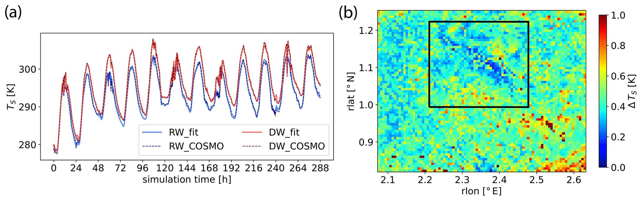
Figure A1(a) Comparison of COSMO domain D3 surface temperature (dashed lines) with the values predicted by the multiple linear regression model (solid lines) described in the main text of Sect. A1 during simulation period T2. The red lines refer to a location within the Dresden Basin (site DW) and the blue lines to a location on an adjacent hill (site RW). (b) Mean absolute error (MAE) of the regressed surface temperature over the domain D3 area during simulation period T2. The black box indicates the CAIRDIO domain D4.
A2 Anelastic approximation, cloud microphysics, and radiative transfer
In our previous model version, the Boussinesq approximation for an incompressible fluid was used to consider buoyancy effects. The error introduced by the assumption of a constant-in-space air density restricted model applications to shallow computation domains. This restriction is now alleviated with the use of the anelastic approximation, which uses a reference density vertical profile (ρ0:=ρ0(z)). In addition to ρ0, the model requires air pressure p for the optional computation of warm clouds and radiative transfer, which are not included in a previous model version and are further described below. In contrast to ρ0, p may vary also horizontally. As with all other external meteorological fields, ρ0 and p are derived from the mesoscale fields of the driving COSMO simulation. In the previous Sect. A1, a multiple linear regression model to spatially downscale, among other surface variables, the surface pressure field pS is presented. Using reconstructed pS together with the spatially (trilinear) interpolated virtual temperature field Tv of COSMO, the downscaled fields p and ρ0 are obtained by vertical integration of the hydrostatic balance, starting from the surface hS:
where g=9.81 m s−1 is the gravity acceleration and Rd=287 the ideal gas constant of dry air. Note that Eq. (A2) is applied to each vertical column of the CAIRDIO grid separately, so that ρ still requires horizontal averaging along planes of to obtain ρ0.
For the simulation of low-altitude clouds and fog formation at temperatures above the freezing point of water, a single-moment bulk warm-cloud microphysics scheme was implemented. This scheme uses only cloud liquid water and rain water as cloud and precipitation constituents. Relevant microphysical processes include condensation and evaporation of cloud water, auto-conversion and collection of cloud water to form rain water, and evaporation and sedimentation of rain water. The bulk parameterizations treat these processes in terms of the mass-mixing ratios of water vapor qv, cloud water qc, and rain water qr. The parameterizations are basically adopted from Klemp and Wilhelmson (1978). The cloud microphysics scheme is applied at each model time step after the integration of all other prognostic tendencies (advection, diffusion, etc.) of the meteorological variables. The first process to be treated in the microphysics scheme is rain formation:
with , k2=2.2, and the threshold cloud water mixing ratio for auto conversion .
Thereafter, in general, qv and qc can be out of equilibrium, i.e., qv may either exceed saturation with respect to liquid water , or clouds may be present (qc>0) in sub-saturated conditions . The condensation or evaporation rate to restore thermodynamic equilibrium is computed by a saturation adjustment technique, which numerically solves the following equation for δT using Halley's third-order method:
Here, J kg−1 is the heat of evaporation, the prognostic model temperature using interpolated pressure p, Pa, , and Rw=462 the gas constant of water vapor. The saturation vapor pressure is computed according to an updated formula of Arden Buck:
The condensation or evaporation rate then follows by
The last microphysical process considered is rain evaporation, whose parameterization is also taken from Klemp and Wilhelmson (1978):
where ρ0 and p are provided in units of g cm−3 and hPa, respectively. Note that since Eq. (A8) is applied after the saturation adjustment, it can be only effective in sub-saturated conditions. The sedimentation of rain droplets is not directly considered in the microphysics scheme but is accounted for by an additional vertical advection step following the 3-D standard advection routine for qr. As the terminal fall velocity vr can significantly exceed the average wind speed, this advection step is split into a variable number of sub-steps so as not to impair model stability or integration efficiency.
The realistic simulation of low-altitude stratiform clouds requires the consideration of radiative processes, in particular the enhanced radiative cooling of the cloud tops. For this purpose, an external library of the Rapid Radiative Transfer Model (RRTM) (Mlawer et al., 1997) is used. RRTM is based on the two-stream approximation and computes heating rates for long- and short-wave interactions within each layer of an atmospheric column. Aside from the vertical profiles of air pressure and temperature, RRTM requires profiles of the atmospheric gaseous composition. The contributions of the greenhouse gases methane, nitrous oxide, ozone, and a multitude of hydrofluorocarbon species are considered by a spatially constant effective carbon dioxide molar mixing ratio, which is assumed to be 500 ppmv and thus higher than the current average value of about 410 ppmv. As non-gaseous constituents, RRTM can consider aerosols and clouds, but in our current framework only clouds are considered by the mixing ratios of liquid water and cloud ice, and the effective particle radii, which are assumed to be 10 µm for cloud water and 30 µm for cloud ice. While additionally considering urban aerosol radiative effects can decrease the model temperature bias (e.g., Strömberg et al., 2023), it would significantly increase model complexity and also simulation time, because other aerosol species aside from the currently simulated BC had to be included. The radiative transfer equations are solved for the entire vertical extent of the troposphere and lower stratosphere, but of the required input data for clouds, only qc is provided with high spatial resolution within the vertical height range of the CAIRDIO computation domain. Therefore, ice clouds and other liquid-water clouds above the domain top are interpolated from the hosting COSMO simulation with lower spatial and temporal accuracy. Similarly, profiles of pressure, specific humidity, and temperature are filled in with COSMO data above the CAIRDIO domain top.
The model code of CAIRDIO v2.1 and utilities for data pre-processing used in this study are accessible in release under license GPL v3 and later at https://doi.org/10.5281/zenodo.7409604 (Weger et al., 2022b).
All model results and observational data published in this study are accessible under license GPL v3 and later at https://doi.org/10.5281/zenodo.8388993 (Weger and Heinold, 2023).
The supplement related to this article is available online at: https://doi.org/10.5194/acp-23-13769-2023-supplement.
MW contributed to study conceptualization, execution and evaluation of model runs, and paper writing. BH supervised the study, provided technical support, and contributed to the proofreading.
The contact author has declared that neither of the authors has any competing interests.
Publisher’s note: Copernicus Publications remains neutral with regard to jurisdictional claims made in the text, published maps, institutional affiliations, or any other geographical representation in this paper. While Copernicus Publications makes every effort to include appropriate place names, the final responsibility lies with the authors.
This article is part of the special issue “Air quality research at street level – Part II (ACP/GMD inter-journal SI)”. It is not associated with a conference.
Recent German-wide emission data were provided by the German Environment Agency (Umweltbundesamt, UBA). A special thanks goes to Uwe Wolf from the Saxon State Office for Environment, Agriculture and Geology (Sächsisches Landesamt für Umwelt, Landwirtschaft und Geologie, LfULG) for providing line emissions for road transport in Dresden. Measurements of BC and other meteorological variables from the air-monitoring sites consulted were provided by the LfULG. Building geometries and orography (DGM1) are available from the State Enterprise for Geographic Information and Surveying Saxony (GeoSN). We thank the DWD for the good cooperation and support. We further thank the three anonymous referees and Michael Jähn (ETH Zurich) for their valuable comments.
The publication of this article was funded by the Open Access Fund of the Leibniz Association.
This paper was edited by Ashu Dastoor and reviewed by three anonymous referees.
Boering, K., Wofsy, S., Daube, B., Schneider, H., Loewenstein, M., Podolske, J., and Conway, T.: Stratospheric mean ages and transport rates from observations of carbon dioxide and nitrous oxide, Science, 274, 1340—1343, https://doi.org/10.1126/science.274.5291.1340, 1996. a
Chemel, C. and Burns, P.: Pollutant Dispersion in a Developing Valley Cold-Air Pool, Bound.-Lay. Meteorol., 154, 391–408, https://doi.org/10.1007/s10546-014-9984-5, 2015. a, b
Cheng, Z., Morgenstern, M., Zhang, B., Fraund, M., Lata, N. N., Brimberry, R., Marcus, M. A., Mazzoleni, L., Fialho, P., Henning, S., Wehner, B., Mazzoleni, C., and China, S.: Particle phase-state variability in the North Atlantic free troposphere during summertime is determined by atmospheric transport patterns and sources, Atmos. Chem. Phys., 22, 9033–9057, https://doi.org/10.5194/acp-22-9033-2022, 2022. a
Deardorff, J. W.: The use of subgrid transport equations in a three-dimensional model of atmospheric turbulence, J. Fluid. Eng., 95, 429–438, https://doi.org/10.1115/1.3447047, 1973. a
Deleersnijder, É., Campin, J. M., and Delhez, É. J. M.: The concept of age in marine modelling I. Theory and preliminary model results, J. Marine Syst., 28, 229–267, https://doi.org/10.1016/S0924-7963(01)00026-4, 2001. a, b, c, d, e, f
Deleersnijder, E., Draoui, I., Lambrechts, J., Legat, V., and Mouchet, A.: Consistent boundary conditions for age calculations, Water, 12, 1–29, https://doi.org/10.3390/w12051274, 2020. a
Delhez, E. J., Campin, J.-M., Hirst, A. C., and Deleersnijder, E.: Toward a general theory of the age in ocean modelling, Ocean Model., 1, 17–27, https://doi.org/10.1016/S1463-5003(99)00003-7, 1999. a, b
England, M.: The age of water and ventilation timescales in a global ocean model, J. Phys. Oceanogr., 25, 2756–2777, https://doi.org/10.1175/1520-0485(1995)025<2756:TAOWAV>2.0.CO;2, 1995. a
Fast, J. D., Zhong, S., and Whiteman, C. D.: Boundary layer evolution within a canyonland basin. Part II: Numerical simulations of nocturnal flows and heat budgets, J. Appl. Meteorol., 35, 2162–2178, https://doi.org/10.1175/1520-0450(1996)035<2162:BLEWAC>2.0.CO;2, 1996. a
Flemming, J., Huijnen, V., Arteta, J., Bechtold, P., Beljaars, A., Blechschmidt, A.-M., Diamantakis, M., Engelen, R. J., Gaudel, A., Inness, A., Jones, L., Josse, B., Katragkou, E., Marecal, V., Peuch, V.-H., Richter, A., Schultz, M. G., Stein, O., and Tsikerdekis, A.: Tropospheric chemistry in the Integrated Forecasting System of ECMWF, Geosci. Model Dev., 8, 975–1003, https://doi.org/10.5194/gmd-8-975-2015, 2015. a
Hall, T. M. and Plumb, R. A.: Age as a diagnostic of stratospheric transport, J. Geophys. Res.-Atmos., 99, 1059–1070, https://doi.org/10.1029/93JD03192, 1994. a
Hall, T. M. and Waugh, D. W.: Timescales for the stratospheric circulation derived from tracers, J. Geophys. Res.-Atmos., 102, 8991–9001, https://doi.org/10.1029/96JD03713, 1997. a
Han, Q. and Zender, C. S.: Desert dust aerosol age characterized by mass-age tracking of tracers, J. Geophys. Res.-Atmos., 115, 1–11, https://doi.org/10.1029/2010JD014155, 2010. a
Kenjereš, S. and Hanjalić, K.: Combined effects of terrain orography and thermal stratification on pollutant dispersion in a town valley: a T-RANS simulation, J. Turbul., 3, N26, https://doi.org/10.1088/1468-5248/3/1/026, 2002. a
Kleinman, L., Daum, P., Lee, Y.-N., Nunnermacker, L., Springston, S., Weinstein-Lloyd, J., Hyde, P., Doskey, P., Rudolph, J., Fast, J., and Berkowitz, C.: Photochemical age determinations in the Phoenix metropolitan area, J. Geophys. Res., 108, 1–14, https://doi.org/10.1029/2002JD002621, 2003. a
Klemp, J. B. and Wilhelmson, R. B.: The simulation of three-dimensional convective storm dynamics, J. Atmos. Sci., 35, 1070–1096, https://doi.org/10.1175/1520-0469(1978)035<1070:TSOTDC>2.0.CO;2, 1978. a, b
Lehner, M. and Gohm, A.: Idealised simulations of daytime pollution transport in a steep valley and its sensitivity to thermal stratification and surface albedo, Bound.-Lay. Meteorol., 134, 327–351, https://doi.org/10.1007/s10546-009-9442-y, 2010. a
Lian, T. and Chen, D.: An evaluation of rotated EOF analysis and its application to tropical pacific SST variability, J. Climate, 25, 5361–5373, https://doi.org/10.1175/JCLI-D-11-00663.1, 2012. a
Ludwig, F. L., Horel, J., and Whiteman, C. D.: Using EOF Analysis to Identify Important Surface Wind Patterns in Mountain Valleys, J. Appl. Meteorol., 43, 969–983, https://doi.org/10.1175/1520-0450(2004)043<0969:UEATII>2.0.CO;2, 2004. a
McKee, T. B. and O'Neal, R. D.: The role of valley geometry and energy budget in the formation of nocturnal valley winds, J. Appl. Meteorol. Clim., 28, 445–456, https://doi.org/10.1175/1520-0450(1989)028<0445:TROVGA>2.0.CO;2, 1989. a
Mercier, C. and Delhez, E.: Consistent computation of the age of water parcels using CART, Ocean Model., 35, 67–76, https://doi.org/10.1016/j.ocemod.2010.06.005, 2010. a
Mlawer, E. J., Taubman, S. J., Brown, P. D., Iacono, M. J., and Clough, S. A.: Radiative transfer for inhomogeneous atmospheres: RRTM, a validated correlated-k model for the longwave, J. Geophys. Res.-Atmos., 102, 16663–16682, https://doi.org/10.1029/97JD00237, 1997. a
Pisso, I., Sollum, E., Grythe, H., Kristiansen, N. I., Cassiani, M., Eckhardt, S., Arnold, D., Morton, D., Thompson, R. L., Groot Zwaaftink, C. D., Evangeliou, N., Sodemann, H., Haimberger, L., Henne, S., Brunner, D., Burkhart, J. F., Fouilloux, A., Brioude, J., Philipp, A., Seibert, P., and Stohl, A.: The Lagrangian particle dispersion model FLEXPART version 10.4, Geosci. Model Dev., 12, 4955–4997, https://doi.org/10.5194/gmd-12-4955-2019, 2019. a
Rendón, A. M., Salazar, J. F., and Wirth, V.: Daytime air pollution transport mechanisms in stable atmospheres of narrow versus wide urban, Environ. Fluid Mech., 20, 1101–1118, https://doi.org/10.1007/s10652-020-09743-9, 2020. a, b
Roberto, B., Roberto, B., Sonia, M., and Paolo, Z.: Formulation of the Lagrangian particle model LAPMOD and its evaluation against Kincaid SF6 and SO2 datasets, Atmos. Environ., 163, 87–98, https://doi.org/10.1016/j.atmosenv.2017.05.039, 2017. a
Sabatier, T., Largeron, Y., Paci, A., Lac, C., Rodier, Q., Canut, G., and Masson, V.: Semi-idealized simulations of wintertime flows and pollutant transport in an Alpine valley. Part II: Passive tracer tracking, Q. J. Roy. Meteor. Soc., 146, 827–845, https://doi.org/10.1002/qj.3710, 2020. a, b
Schubert, S., Grossman-Clarke, S., and Martilli, A.: A double-canyon radiation scheme for multi-layer urban canopy models, Bound.-Lay. Meteorol., 145, 439–468, https://doi.org/10.1007/s10546-012-9728-3, 2012. a
Stohl, A., Forster, C., Eckhardt, S., Spichtinger, N., Huntrieser, H., Heland, J., Schlager, H., Wilhelm, S., Arnold, F., and Cooper, O.: A backward modeling study of intercontinental pollution transport using aircraft measurements, J. Geophys. Res.-Atmos., 108, 1–18, https://doi.org/10.1029/2002JD002862, 2003. a
Strömberg, J., Li, X., Kurppa, M., Kuuluvainen, H., Pirjola, L., and Järvi, L.: Effect of radiation interaction and aerosol processes on ventilation and aerosol concentrations in a real urban neighbourhood in Helsinki, Atmos. Chem. Phys., 23, 9347–9364, https://doi.org/10.5194/acp-23-9347-2023, 2023. a
Troude, F., Dupont, E., Carissmo, B., and Flossmann, A.: Mesoscale Meteorological Simulations In Paris: Comparisons With Observations During The Experiment Eclap, Bound.-Lay. Meteorol., 99, 21–51, https://doi.org/10.1023/A:1018770711016, 2001. a
Wallace, J., Corr, D., and Kanaroglou, P.: Topographic and spatial impacts of temperature inversions on air quality using mobile air pollution surveys, Sci. Total Environ., 408, 5086–5096, https://doi.org/10.1016/j.scitotenv.2010.06.020, 2010. a
Weger, M. and Heinold, B.: CAIRDIO simulation results and observational data for Dresden (1.0), Zenodo [data set], https://doi.org/10.5281/zenodo.8388993, 2023. a
Weger, M., Knoth, O., and Heinold, B.: An urban large-eddy-simulation-based dispersion model for marginal grid resolutions: CAIRDIO v1.0, Geosci. Model Dev., 14, 1469–1492, https://doi.org/10.5194/gmd-14-1469-2021, 2021. a, b
Weger, M., Baars, H., Gebauer, H., Merkel, M., Wiedensohler, A., and Heinold, B.: On the application and grid-size sensitivity of the urban dispersion model CAIRDIO v2.0 under real city weather conditions, Geosci. Model Dev., 15, 3315–3345, https://doi.org/10.5194/gmd-15-3315-2022, 2022a. a, b, c, d, e, f
Weger, M., Knoth, O., and Heinold, B.: CAIRDIO city-scale air dispersion model with diffusive obstacles, Zenodo [code], https://doi.org/10.5281/zenodo.6075354, 2022b. a
Weigel, A. P., Chow, F. K., Rotach, M. W., Street, R. L., and Xue, M.: High-resolution large-eddy simulations of flow in a steep alpine valley. Part II: Flow structure and heat budgets, J. Appl. Meteorol. Clim., 45, 87–107, https://doi.org/10.1175/JAM2323.1, 2006. a
Whiteman, C. D.: Observations of thermally developed wind systems in mountainous terrain, in: Atmospheric Processes over Complex Terrain, edited by: Blumen, W., 5–42, American Meteorological Society, Boston, MA, https://doi.org/10.1007/978-1-935704-25-6_2, 1990. a
Whiteman, C. D., McKee, T. B., and Doran, J. C.: Boundary layer evolution within a canyonland basin. Part I: Mass, heat, and moisture budgets from observations, J. Appl. Meteorol., 35, 2145–2161, https://doi.org/10.1175/1520-0450(1996)035<2145:BLEWAC>2.0.CO;2, 1996. a
Wolke, R., Schröder, W., Schrödner, R., and Renner, E.: Influence of grid resolution and meteorological forcing on simulated European air quality: A sensitivity study with the modeling system COSMO-MUSCAT, Atmos. Environ., 53, 110–130, https://doi.org/10.1016/j.atmosenv.2012.02.085, 2012. a
Zeeman, M., Holst, C. C., Kossmann, M., Leukauf, D., Münkel, C., Philipp, A., Rinke, R., and Emeis, S.: Urban atmospheric boundary-layer structure in complex topography: An empirical 3D case study for Stuttgart, Germany, Front. Earth Sci., 10, 1–19, https://doi.org/10.3389/feart.2022.840112, 2022. a
Zhang, W. G., Wilkin, J. L., and Schofield, O. M. E.: Simulation of water age and residence time in New York Bight, J. Phys. Oceanogr., 40, 965–982, https://doi.org/10.1175/2009JPO4249.1, 2010. a