the Creative Commons Attribution 4.0 License.
the Creative Commons Attribution 4.0 License.
 | 25 Oct 2023
Atmospheric composition and climate impacts of a future hydrogen economy
Nicola J. Warwick
Alex T. Archibald
Paul T. Griffiths
James Keeble
Fiona M. O'Connor
John A. Pyle
Keith P. Shine
Hydrogen is expected to play a key role in the global energy transition to net zero emissions in many scenarios. However, fugitive emissions of hydrogen into the atmosphere during its production, storage, distribution and use could reduce the climate benefit and also have implications for air quality. Here, we explore the atmospheric composition and climate impacts of increases in atmospheric hydrogen abundance using the UK Earth System Model (UKESM1) chemistry–climate model. Increases in hydrogen result in increases in methane, tropospheric ozone and stratospheric water vapour, resulting in a positive radiative forcing. However, some of the impacts of hydrogen leakage are partially offset by potential reductions in emissions of methane, carbon monoxide, nitrogen oxides and volatile organic compounds from the consumption of fossil fuels. We derive a refined methodology for determining indirect global warming potentials (GWPs) from parameters derived from steady-state simulations, which is applicable to both shorter-lived species and those with intermediate and longer lifetimes, such as hydrogen. Using this methodology, we determine a 100-year global warming potential for hydrogen of 12 ± 6. Based on this GWP and hydrogen leakage rates of 1 % and 10 %, we find that hydrogen leakage offsets approximately 0.4 % and 4 % respectively of total equivalent CO2 emission reductions in our global hydrogen economy scenario. To maximise the benefit of hydrogen as an energy source, emissions associated with hydrogen leakage and emissions of the ozone precursor gases need to be minimised.
-
Please read the editorial note first before accessing the article.
-
Article
(3701 KB)
-
Supplement
(486 KB)
-
Please read the editorial note first before accessing the article.
- Article
(3701 KB) - Full-text XML
-
Supplement
(486 KB) - BibTeX
- EndNote


The adoption of low-carbon hydrogen (H2) as an energy source could lead to substantial reductions in carbon dioxide emissions and a significant climate benefit. However, increasing levels of hydrogen in the atmosphere as a result of fugitive emissions from a hydrogen economy will affect atmospheric composition (e.g. Prather, 2003). It is important that the atmospheric implications of potential changes in hydrogen emissions are investigated in detail before the implementation of widespread hydrogen use.
The hydrogen abundance in the atmosphere increased over the twentieth century (Patterson et al., 2021) and today has a mixing ratio of around 530 parts per billion (ppb), with a small interhemispheric gradient (±20 ppb) (Novelli et al., 1999; Patterson et al., 2021). Fossil fuel combustion and biomass burning account for approximately 50 % of the current total global hydrogen source, with the remainder arising from the oxidation of methane (CH4) and volatile organic compounds (VOCs) in the atmosphere (e.g. Ehhalt and Rohrer, 2009; Pieterse et al., 2013; Grant et al., 2010). Hydrogen removal is dominated primarily by uptake to soils and reaction with hydroxyl radicals (OH). OH is the main atmospheric oxidising agent, and if hydrogen emissions were to increase, subsequent changes in the OH concentration could alter the lifetimes of important atmospheric greenhouse gases. Therefore, whilst hydrogen itself is not radiatively active, it can act as an indirect greenhouse gas.
An increase in the tropospheric concentration of hydrogen reduces the availability of OH via Reaction (R1). Reductions in tropospheric OH will result in increases in the atmospheric lifetime of CH4 and its abundance (Derwent et al., 2001; Schultz et al., 2003; Warwick et al., 2004; Derwent et al., 2020; Field and Derwent, 2021) since the major atmospheric sink of CH4 is through reaction with OH (Reaction R2).
The oxidation of both hydrogen and CH4 in the troposphere can lead to the generation of ozone, which impacts both climate and air quality (e.g. Archibald et al., 2020a; Schultz et al., 2003). In the stratosphere, oxidation of hydrogen and methane will lead to increases in stratospheric water vapour with potential implications for climate and stratospheric ozone (e.g. Tromp et al., 2003; Warwick et al., 2004). Increases in atmospheric hydrogen could also influence stratospheric ozone recovery through the production of HOx radicals (i.e. OH + HO2), which are involved in ozone destruction cycles.
The extent to which future changes in hydrogen might affect atmospheric composition and climate will depend upon the level of hydrogen leakage and the ultimate size of a future hydrogen economy. In addition, emission reductions in species currently emitted by the production and consumption of fossil fuels, including methane, CO, NOx (i.e. NO + NO2) and volatile organic compounds (VOCs), will also induce feedbacks on atmospheric composition (e.g. Jacobson, 2008). There is significant uncertainty in the size of a future hydrogen economy, and the leakage rates and emission reductions in other species are uncertain, depending on the forms of new technology implemented (e.g. Frazer-Nash Consultancy, 2022; Lewis, 2021).
Here, we report, using calculations made with the UK Earth System Model (UKESM1) (Sellar et al., 2020) chemistry–climate model, on the climate and atmospheric composition effects of a range of different atmospheric hydrogen boundary conditions, consistent with a range of different scenarios for a future hydrogen economy. The work presented here is both based on and an extension of the work presented in Warwick et al. (2022). We determine changes in effective radiative forcing (ERF) and present an improved estimate of the hydrogen global warming potential (GWP), accounting for composition changes in both the troposphere and the stratosphere. As part of our GWP calculations, we present a refined methodology for calculating indirect GWPs from steady-state simulations, appropriate for use with both short-lived and longer-lived species.
2.1 The UK Earth System Model (UKESM1)
The UK Earth System Model (UKESM1) (Sellar et al., 2020), is a state-of-science Earth system model that couples Earth system modules to the HadGEM3-GC3.1 climate model (Kuhlbrodt et al., 2018; Williams et al., 2018). UKESM1 has a horizontal resolution of 1.875 ∘ in longitude and 1.25 ∘ in latitude and 85 vertical levels extending from the surface to 85 km. Atmospheric composition changes are calculated using the UK Chemistry and Aerosols (UKCA) atmospheric chemistry module, which includes a coupled stratospheric–tropospheric chemistry scheme (Archibald et al., 2020b) and an interactive two-moment aerosol scheme (Mulcahy et al., 2020). UKCA includes the emissions of nine chemical species: nitric oxide (NO), carbon monoxide (CO), formaldehyde (HCHO), ethane (C2H6), propane (C3H8), acetaldehyde (MeCHO), acetone (Me2CO), isoprene (C5H8) and methanol (MeOH), while surface mixing ratios of CH4, N2O, CFC-11 (CFCl3), CFC-12 (CF2Cl2), CH3Br, H2 and COS are prescribed. The photochemical sources and sinks of H2 and CH4 are fully interactive, but the use of the lower boundary condition (LBC) fixes the atmospheric burden of H2 and CH4. LBCs are widely used in chemistry–climate models as they (1) allow the observed burdens of intermediate lifetime (t > 1 year) species to be imposed, bypassing the need to include emissions, and (2) remove the need for a long spin-up for longer-lived species burdens to reach a steady state. By using an LBC, any chemical feedbacks that would affect the burden of these species are overwritten. However, the effect of feedbacks on the steady-state burden can be computed through quantification of the appropriate chemical feedback factors (see, for example, Heimann et al., 2020, for a discussion on how we have done this for methane).
2.2 Box model
Atmospheric box model simulations were performed using a coupled H2–CH4–CO–OH chemical scheme to link lower boundary condition values of H2 with fugitive H2 emission rates and obtain CH4 lower boundary conditions for use in the UKESM1 experiments. In addition, the box model was used for extensive testing of the framework for GWP calculations.
Our box modelling approach is described in more detail in Warwick et al. (2022), is similar to the approach described in Prather (1994) and is used in other studies (Heimann et al., 2020; Nisbet et al., 2020). The model was initialised with realistic values for total methane emissions (585 Tg (CH4) yr−1), CO (1300 Tg(CO) yr−1) and H2 (80 Tg(H2) yr−1) (e.g. Saunois et al., 2020; Pieterse et al., 2013; Zheng et al., 2019) and was found to give methane and H2 levels in broad agreement with present-day levels – 1865 ppb CH4, 552 ppb H2 and 101 ppb CO, as well as a CH4 lifetime of 9.9 years, which is within the range of observationally derived values.
2.3 Hydrogen economy scenarios
2.3.1 Changes in the abundance of atmospheric H2 in a hydrogen economy
The increase in abundance of atmospheric H2 in a future hydrogen economy is not well constrained due to uncertainties in fugitive emissions, which will depend on the ultimate size of the hydrogen economy, H2 leakage rates and uncertainties in the amount of H2 undergoing uptake by soils. To guide our model scenarios, we estimate how emissions of H2 and other species may change in response to a switch from fossil fuel to hydrogen technologies in an illustrative hydrogen economy scenario. In this scenario, approximately 23 % of global energy consumption (about 133 EJ) is supplied by hydrogen (BP, 2020). We, here, assume that in the buildings sector, the transport sector and the power generation sector, 100 %, 50 % and 10 % respectively of the final consumption of fossil fuels switches to hydrogen. The lower percentages for the transport sector and the power generation sector reflect the smaller role hydrogen is assumed to play in these energy sectors due to the existence of low-carbon alternatives such as electric vehicles, wind power and solar power, as well as alternative storage options such as pumped hydro, batteries and compressed air (e.g. Staffell et al., 2019). New hydrogen technologies are assumed to have the same energy efficiency as the fossil fuel technology they are replacing (Staffell et al., 2019), except for in the transport sector, where we assume diesel vehicles and petrol vehicles with an average tank-to-wheel energy efficiency of 30 % will be replaced by vehicles using hydrogen fuel cells with an average efficiency of 50 %. Using a net calorific value of 1 kg H2 = 33.3 kWh, approximately 860 Tg H2 yr−1 would be required to provide the energy consumption outlined above.
H2 leakage rates of the infrastructure associated with a hydrogen economy are uncertain and will depend on many factors (e.g. E4tech, Ltd, 2019). However, all else being equal, H2 leakage rates of the infrastructure associated with a hydrogen economy are likely to be higher than the leakage rates of natural gas, owing to the small molecule size of hydrogen. A recent study, looking at the US natural gas supply chain, indicated natural gas leaks of around 2.3 % of gross gas production, which is ∼ 60 % higher than the US EPA inventory estimate (Alvarez et al., 2018). H2 leakage rates of 1 % and 10 % (which represent the range of values used in previous studies e.g. Shultz et al., 2003; Warwick et al., 2004) would lead to additional H2 emissions of 9 and 96 Tg H2 yr−1 respectively based on a hydrogen economy supplying 23 % of total present-day energy consumption.
Table 1List of UKESM1 hydrogen economy scenarios employing different H2 lower boundary conditions (LBCs). The CH4 LBC used in the scenarios, not including a CH4 feedback, is 1835 ppb (2014 year level). In scenarios including a CH4 feedback (CH4f), the CH4 LBC is determined using box modelling. Reductions in O3 precursor emissions (O3pre) are described in Sect. 2.3.2.
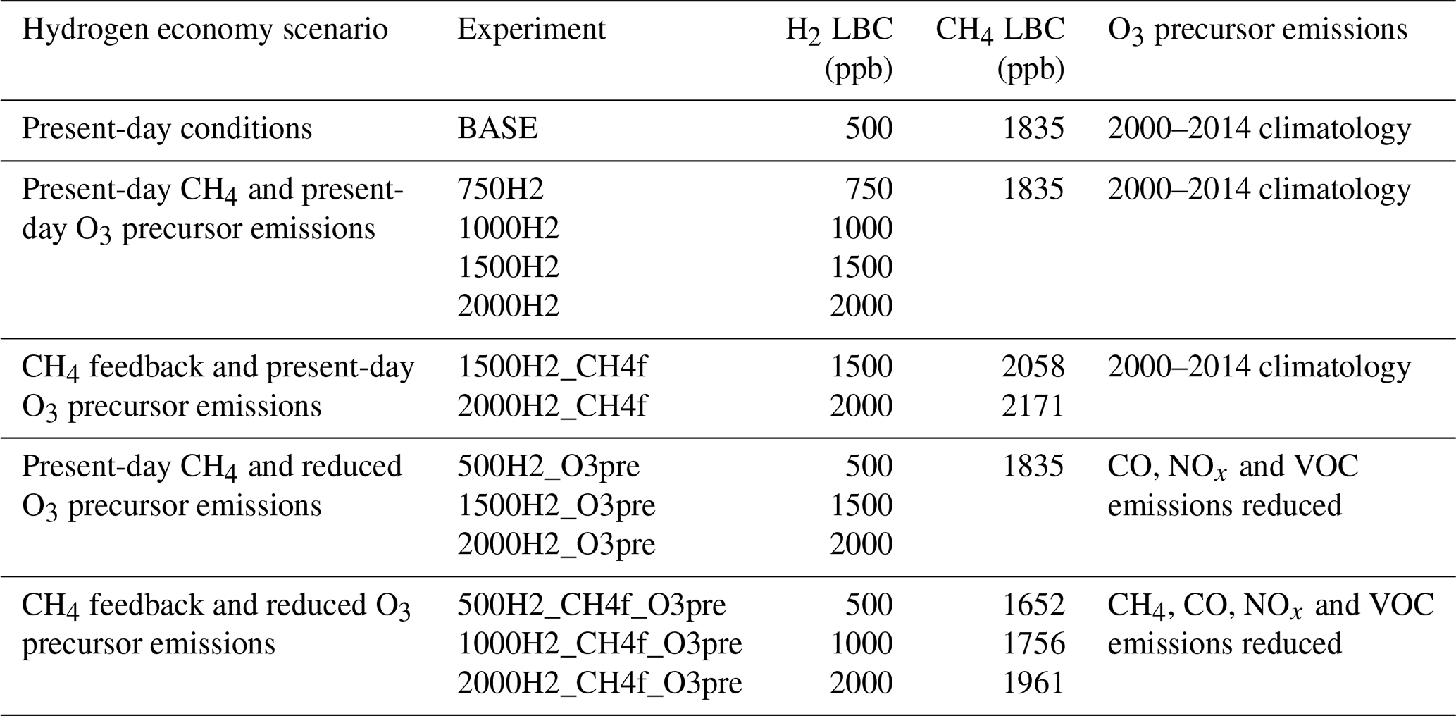
We bypass some of the uncertainties in H2 leakage rates, the ultimate size of the hydrogen economy and soil uptake rates, by performing a range of hydrogen economy scenarios with fixed H2 lower boundary mixing ratios. We consider scenarios with H2 lower boundary conditions ranging from 500 to 2000 ppb (i.e. increases relative to present-day mixing ratios of 0 to 1500 ppb), which we believe span many of these uncertainties (see Table 1). For example, based on the size of a hydrogen economy under the conditions outlined above, and assuming the magnitude of the soil sink increases in line with the increase in H2 mixing ratios (i.e. a constant deposition velocity), box model simulations indicate H2 lower boundary conditions of 750, 1000 and 1500 ppb represent H2 leakage rates of about 3 %, 7 % and 13 % respectively (see Sect. 2.2 for further details on the box modelling). However, these H2 lower boundary conditions would also be consistent with other fractions of total energy supplied by H2, alternative soil sink responses and H2 leakage rates. Use of this range of H2 lower boundary conditions provides a clear signal in the atmospheric response to increased H2 mixing ratios relative to interannual variability and allows us to explore the linearity of the atmospheric response to increasing H2. Note that our 2000 ppb H2 scenario should be considered an extreme end member designed to assess the linearity of the atmospheric response to increasing atmospheric H2, rather than a projection of potential future atmospheric H2 levels in a hydrogen economy.
2.3.2 Changes in CH4, CO, NOx and VOC emissions in a hydrogen economy
To determine the associated changes in CH4, CO, NOx and VOC emissions, further assumptions are required about the new technology employed, in addition to the percentage of different energy sectors switching to H2. In the building sector, we assume that H2 will be combusted and NOx emissions will be limited such that they remain unaltered (despite the potential for higher NOx emissions from the increased flame temperature), whilst emissions of CH4, CO and VOCs are eliminated. In the transport sector, we assume a 50 % reduction in emissions of CH4, CO, NOx and VOCs based on 50 % of oil-based transport being replaced by hydrogen fuel cells. In the power sector, we assume that stored hydrogen will be used to generate 30 % of the electricity that is currently generated using natural gas via combustion and that NOx will remain unaltered, whilst emissions of CH4, CO and VOCs are scaled appropriately. CH4 emissions associated with energy production are also scaled according to the decreased use of CH4 where it has been replaced by H2. The assumptions above lead to reductions in CH4, CO and NO2 emissions of 43, 259 and 19 Tg yr−1 (see Warwick et al., 2022, for further details).
Emission reductions for CO, NOx and VOCs are determined by applying a uniform global-scaling factor to emissions from the specific energy sectors mentioned by Gidden et al. (2019) where hydrogen is assumed to play a role. The emission reductions determined for CH4 are converted to a change in the CH4 lower boundary condition for UKESM1 using the box model (see Sect. 2.2). To separate the atmospheric impacts of increasing hydrogen mixing ratios, the feedback on the CH4 abundance and changes in the emissions of other species emitted by the consumption of fossil fuels, four different sets of hydrogen economy model simulations are performed as described in Table 1.
2.3.3 Model simulations
For the BASE simulation, all boundary conditions are taken from the recently developed Coupled Model Intercomparison Project, Phase 6 (CMIP6), data set and we assume an H2 LBC of 500 ppb. Climatological boundary conditions for sea-surface temperatures, sea-ice extent and anthropogenic and natural emissions are averaged over the years 2000–2014. In the first set of hydrogen economy scenarios, we consider changes in the atmospheric H2 abundance only. In these simulations, the methane abundance is fixed at 1835 ppb (the 2014 year level) and does not respond to changes in the methane lifetime. In the second set of hydrogen economy scenarios, we include the methane response to changes in atmospheric H2 via the impact of H2 on OH and the methane lifetime. The methane LBCs in these simulations are determined via a series of box model simulations where H2 is varied (see Sect. 2.2). In the third set of hydrogen economy scenarios, we consider reductions in emissions of the ozone precursors, CO, NOx and VOCs, from reduced fossil fuel use, whilst the methane abundance is fixed at 1835 ppb. The fourth set of hydrogen economy scenarios includes decreases in the emissions of CH4, CO, NOx and VOCs from reduced fossil fuel use, in addition to the feedback of changes in the methane lifetime on the methane abundance. In these scenarios, we assume that all hydrogen will be green hydrogen with no emissions of other species associated with the H2 production method. In the case that blue or grey hydrogen is used, it is possible methane emissions may increase due to emissions occurring during hydrogen production (e.g. Bertagni et al., 2022). Each simulation was run for 40 years using annually repeating conditions with the final 25 years of each simulation used for analysis and the initial 15 years treated as a spin-up period.
3.1 Atmospheric composition impacts following changes in hydrogen and methane
To determine the indirect radiative impact of hydrogen, we need to understand how CH4, O3 and H2O will change, per unit emission of H2. Those changes will depend not only on how H2 changes, but also on changes in species emitted from the production and use of fossil fuel. The scenario space is particularly complex and our scenarios should not be regarded as predictions. Instead, here, we try to indicate how the composition of radiatively active species might generally change and which changes are linear in the change in H2, looking first at the changes driven by H2 and CH4.
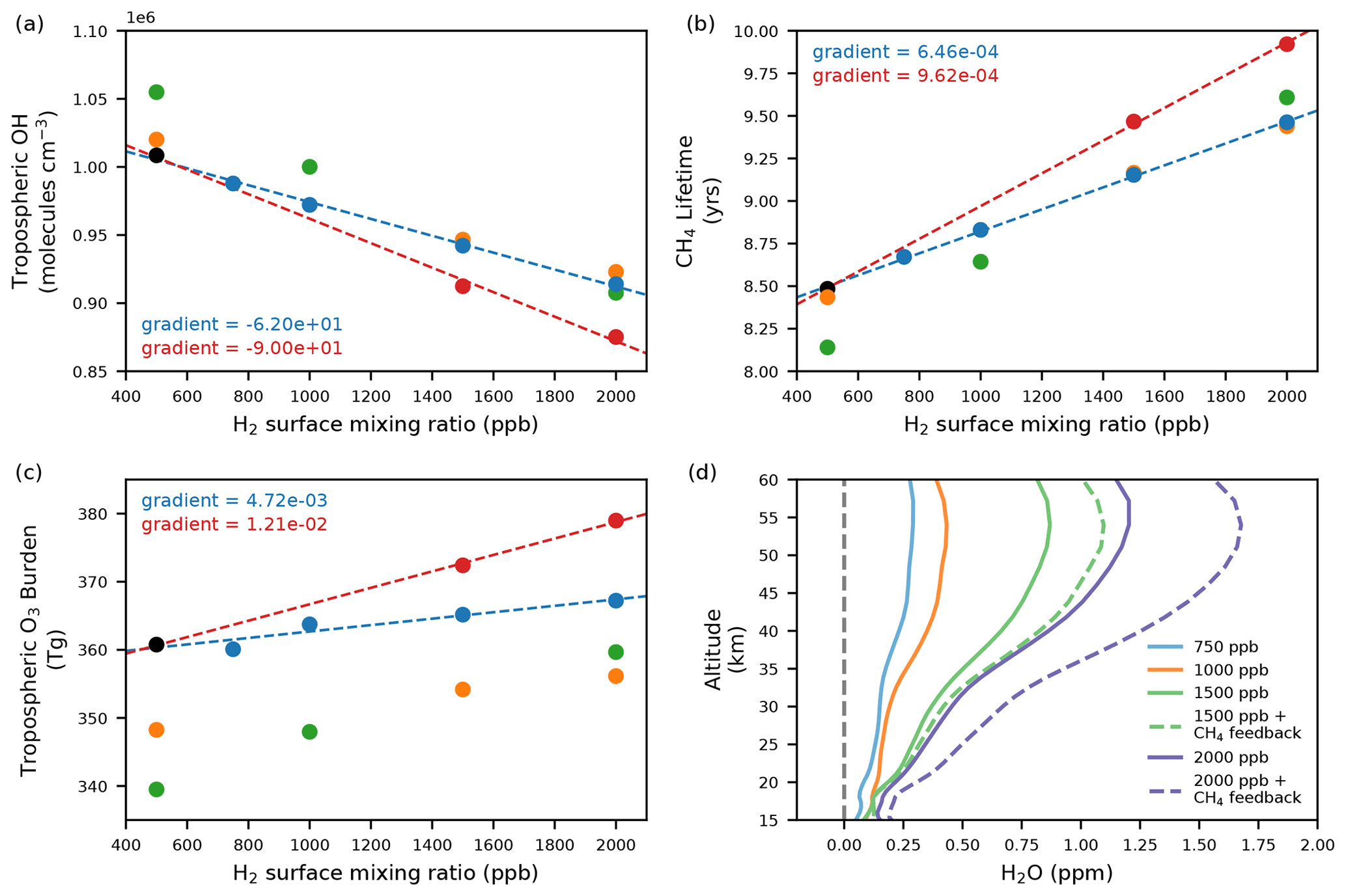
Figure 1The response of (a) mass-weighted tropospheric mean OH, (b) CH4 lifetime with respect to OH, (c) tropospheric O3 and (d) stratospheric water vapour to increasing H2 mixing ratios in UKESM1. In panels (a)–(c), the black circle represents the BASE scenario, the blue circles represent scenarios where the CH4 LBC remains fixed at 2014 levels, the red circles are scenarios where the CH4 LBC is adjusted to account for the change in CH4 lifetime, the orange circles are scenarios including changes in emissions of ozone precursors and the green circles include changes in emissions of CH4 and ozone precursors, as well as adjusted CH4 LBCs to account for the response of the CH4 abundance to changes in the CH4 lifetime. The blue dashed line represents the fit through experiments where the CH4 LBC remains fixed at 2014 levels and the red dashed line is the fit through experiments which include the response of CH4 to changing H2 (and OH). Panel (d) shows the change in the vertical profile of H2O relative to the BASE scenario where the H2 LBC is increased to 750, 1000, 1500 and 2000 ppb. Solid lines represent scenarios where CH4 is fixed at 2014 levels; whereas dashed lines show scenarios where the CH4 LBC is increased to account for the change in CH4 lifetime.
Figure 1 summarises the key composition changes seen in a range of different hydrogen lower boundary mixing ratios when emissions of other species from the fossil fuel industry are held constant (blue and red circles) and when they are reduced (orange and green circles). Decreases in OH, the main atmospheric oxidant, are modelled throughout the troposphere with larger decreases in scenarios with higher H2 abundances (Fig. 1a), consistent with Reaction (R1), being the main atmospheric sink for H2. The change in OH is linear in H2 when both the surface CH4 mixing ratio is held constant (blue circles) and when it is increased to account for the feedback of changes in OH in the methane abundance (red circles). When including this methane feedback, mass-weighted tropospheric mean OH decreases by about 0.90 × 10⁵ molec. cm−3 (or about 10 %) for every 1000 ppb (1 ppm) increase in H2 (Fig. 1a, red circles). When tropospheric mean OH is weighted by reaction with CH4, OH decreases by about 1.8 × 10⁵ molec. cm−3 for every 1 ppm increase in H2. These modelled changes in OH go on to cause a cascade of further composition changes by altering the methane lifetime, production and destruction rates of tropospheric ozone, as well as aerosol nucleation rates and cloud condensation nuclei (CCN) concentrations.
Figure 1b shows the CH4 lifetime with respect to loss by reaction with tropospheric OH as a function of atmospheric H2 and tropospheric OH. In the BASE simulation, the modelled CH4 lifetime with respect to loss by reaction with tropospheric OH is 8.5 years. Adjusting to include losses in the stratosphere (120-year lifetime), but excluding soil loss (160-year lifetime), gives a chemical CH4 lifetime of 7.9 years. This value is lower than the range given for the total chemical methane lifetime in IPCC AR6 (9.7 ± 1.1 years, Szopa et al., 2021) and a present-day total chemical multimodel estimate of 8.4 ± 0.3 years in Stevenson et al. (2020). As atmospheric H2 increases but all other factors remain constant, there is a linear increase in the CH4 lifetime. The methane lifetime increases by 0.64 years for every 1000 ppb (1 ppm) increase in H2 when the methane abundance is held constant (blue circles). However, the methane lifetime increases by 0.96 years for every 1000 ppb increase in H2 when the methane abundance is increased in response to the modelled changes in its lifetime (red circles).
The oxidation of H2 in the troposphere can also affect the levels of ozone (O3) as the HO2 produced through Reaction (R1) can catalyse the interconversion of NOx which drives tropospheric ozone production (e.g. as reviewed in Archibald et al., 2020a),
This is followed by photolysis of NO2 to form ozone,
In addition, changes in OH and HO2 produced via Reaction (R1) influence the destruction of tropospheric ozone by altering the flux through the reaction of O3 with both of these species. Overall, the tropospheric ozone burden increases approximately linearly with atmospheric H2 increase, driven primarily through increases in the reaction HO2 + NO (Reaction R3), which increases by ∼ 7 % when atmospheric H2 increases to 2000 ppb (Fig. 1c). Changes in the ozone budget are documented in Table S2 in the Supplement.
Increased H2 mixing ratios at the surface can also influence stratospheric composition. Increases in H2 and CH4 abundance in the troposphere result in an increased flux of these species to the stratosphere, where their oxidation leads to the production of water vapour. Figure 1d shows the increase in the stratospheric water vapour profile relative to the BASE scenario when tropospheric H2 increases from 500 to 750, 1000, 1500 and 2000 ppb, both where the tropospheric methane abundance remains unchanged and where the methane LBC is adjusted in response to modelled changes in the methane lifetime. When H2 increases to 2000 ppb but CH4 is held constant, stratospheric H2O increases by up to 25 % (> 1 ppm). Note that in our simulations the maximum increase in stratospheric water vapour (occurring at ∼ 55 km) is slightly less than 1 ppm per 1000 ppb increase in surface H2. If the tropospheric methane abundance is increased in line with modelled changes in the CH4 lifetime, larger increases in stratospheric H2O are simulated.
3.2 Atmospheric composition impacts when hydrogen, methane and ozone precursor emissions all change
The impacts discussed above arise from changes in atmospheric H2 abundance and subsequent changes in methane abundance, arising from the feedback of OH on the methane lifetime. Expected reductions in ozone precursor emissions of CO, NOx (which may also increase locally), VOCs and CH4, following a shift to a global hydrogen economy, also have the potential to further impact atmospheric composition. The green circles and the orange circles in Fig. 1a–c show the impact of including these other emission changes with and without the feedback on the methane abundance included respectively. The relationship remains linear for the air-mass-weighted tropospheric mean OH, methane lifetime and tropospheric ozone burden plotted as a function of H2 LBC. In all cases, the gradients remain similar to the corresponding scenarios not including the ozone precursor emission reductions (note the ozone precursor emission changes are the same across all scenarios).
The linear relationships in Fig. 1 show allow the global methane and ozone changes in a range of different hydrogen economy scenarios to be estimated, giving responses to different realisations of a future hydrogen economy. They can also be employed to obtain a GWP for hydrogen (see Sect. 3.4).
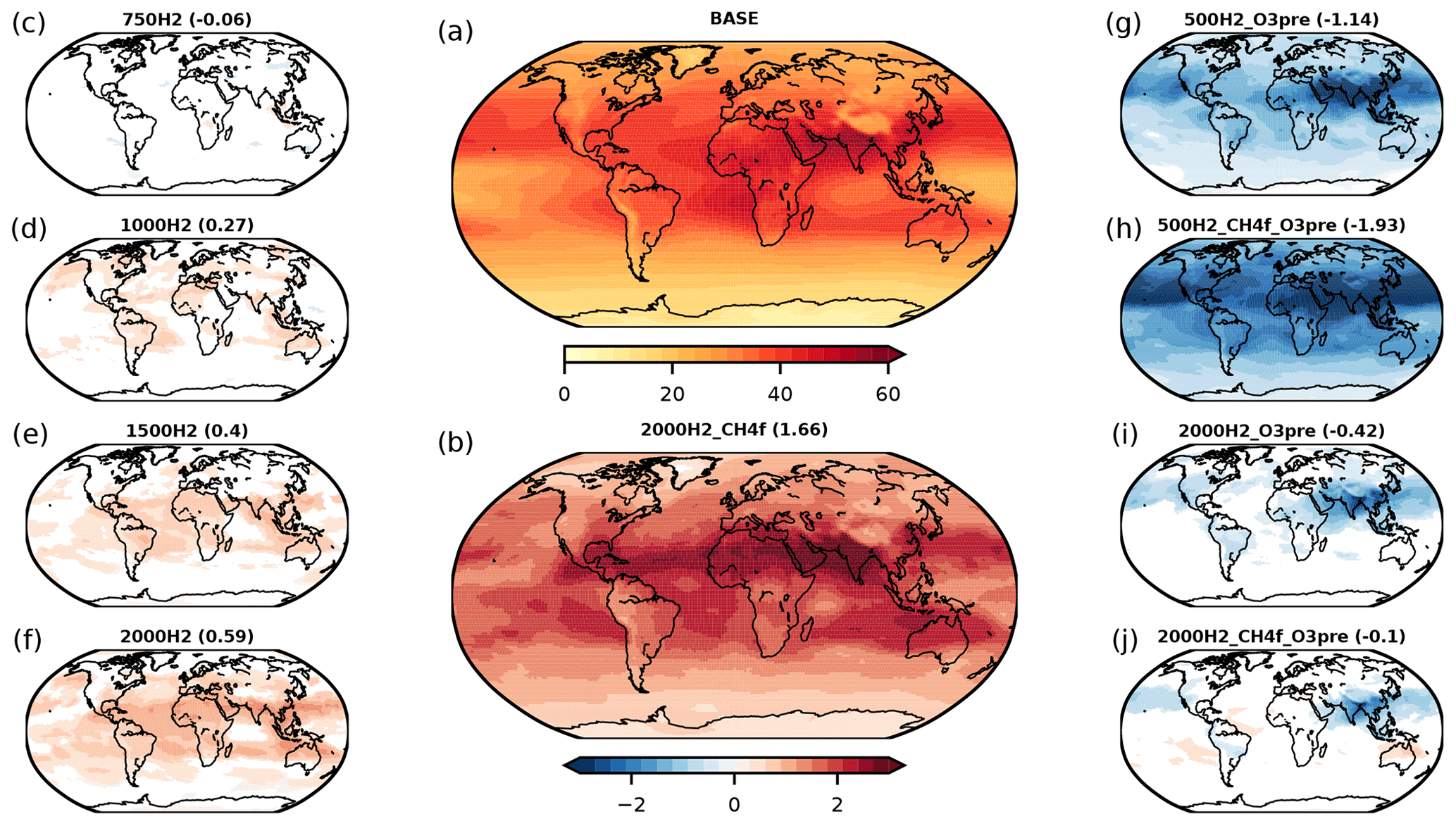
Figure 2Shows the effect of increases in atmospheric H2 on (a) tropospheric ozone column for the BASE scenario (DU); (b) the change in tropospheric ozone column relative to BASE when H2 is increased to 2000 ppb, including the response of the methane abundance to changes in the methane lifetime (DU); (c–f) changes in tropospheric ozone column relative to BASE when H2 mixing ratios are increased, but all other factors including the methane abundance remain fixed; and (g–j) changes in tropospheric ozone column relative to BASE for scenarios including emission reductions in ozone precursors and methane. The numbers above each figure give the change in global mean tropospheric column in DU relative to BASE. Only differences that are statistically significant at the 95 % confidence level are presented.
Some detail on geographical changes in tropospheric ozone in a hydrogen economy is provided in Fig. 2. As the photochemical production of ozone is driven by oxidation of CO, CH4 and VOCs in the presence of NOx, the net regional change in ozone depends not only on how H2 changes, but also on changes in emissions of these species. This sensitivity is demonstrated in Fig. 2.
When H2 increases, so does tropospheric ozone (Fig. 2c to f; see also Fig. 1c). Similarly, when atmospheric methane increases, the effect is to enhance the tropospheric ozone column increase (compare Fig. 2b with f). In contrast, reductions in ozone precursor and CH4 emissions would avoid the significant O3 increases seen in Fig. 2b (see Fig. 2h and j). For example, if there is no H2 leakage, reductions in the other emissions (Fig. 2g and h) lead, as expected, to reductions in tropospheric ozone. When surface H2 reaches 2000 ppb, reductions in the other emissions still lead to modest decreases in ozone (Fig. 2i, j). For example, in the UKESM1 simulation, which assumes a large H2 leakage, with surface mixing ratios of H2 reaching 2000 ppb and emission reductions in CH4, CO, NOx and VOCs, the global mean tropospheric column ozone response is found to be small (−0.1 DU) due to the competing effects outlined above (Fig. 2j). The tropospheric ozone response to a global shift towards a hydrogen economy is therefore strongly influenced by the amount of hydrogen added to the atmosphere through leaks and the co-benefit reductions achieved in CO, NOx, VOC and CH4 emissions.
As shown above, the changes in H2 and methane affect OH which can in turn also influence aerosols in our model simulations. We simulate a linear decrease in both tropospheric air-mass-weighted OH (Fig. 1a) and the OH+SO2 reaction flux, for increasing H2 in the atmosphere. The reduction in the flux through the OH + SO2 reaction results in a shift from the oxidation of SO2 in the gas phase (which contributes towards new particle formation) towards the oxidation of SO2 in the condensed phase (which grows existing particles). Such a shift leads to a reduction in the aerosol number and an increase in aerosol size with impacts on clouds and radiative forcing (see O'Connor et al., 2022, for further details). The modelled decrease in OH following the increase in H2 is coincident with an increase in HO2 (R1 leads to the production of H atoms, which in the troposphere near instantaneously form HO2); thus, H2 acts to increase the HO2 : OH ratio, similar to CO. We find that the HO2 : OH ratio linearly increases with increasing H2 in the atmosphere (from 145 at 500 ppb H2 to 175 at 2000 ppb H2), and, as a result, the H2O2 concentration increases, further enhancing in-cloud oxidation of SO2. Whilst our simulations demonstrate the potential importance of aerosol feedbacks relating to changes in OH, the inclusion of other aerosols, e.g. nitrates, may influence our results and more studies, involving multiple models, are required to constrain the uncertainties involved.
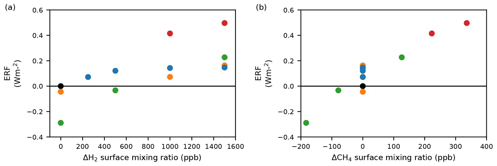
Figure 3The effect of the simulated changes in atmospheric composition on effective radiative forcing (ERF). Panel (a) shows the ERF as a function of H2 and other experimental conditions and panel (b) shows the ERF as a function of CH4 and other experimental conditions. Just as for Fig. 1a–c, the black circle represents the BASE scenario, the blue circles represent scenarios where the CH4 LBC remains fixed at 2014 levels, the red circles are scenarios where the CH4 LBC is adjusted to account for the change in CH4 lifetime, the orange circles are scenarios including changes in emissions of ozone precursors, and the green circles include changes in emissions of CH4 and ozone precursors, as well as adjusted CH4 LBCs to account for the response of the CH4 abundance to changes in the CH4 lifetime. Note that none of the calculated ERFs include anticipated reductions in CO2.
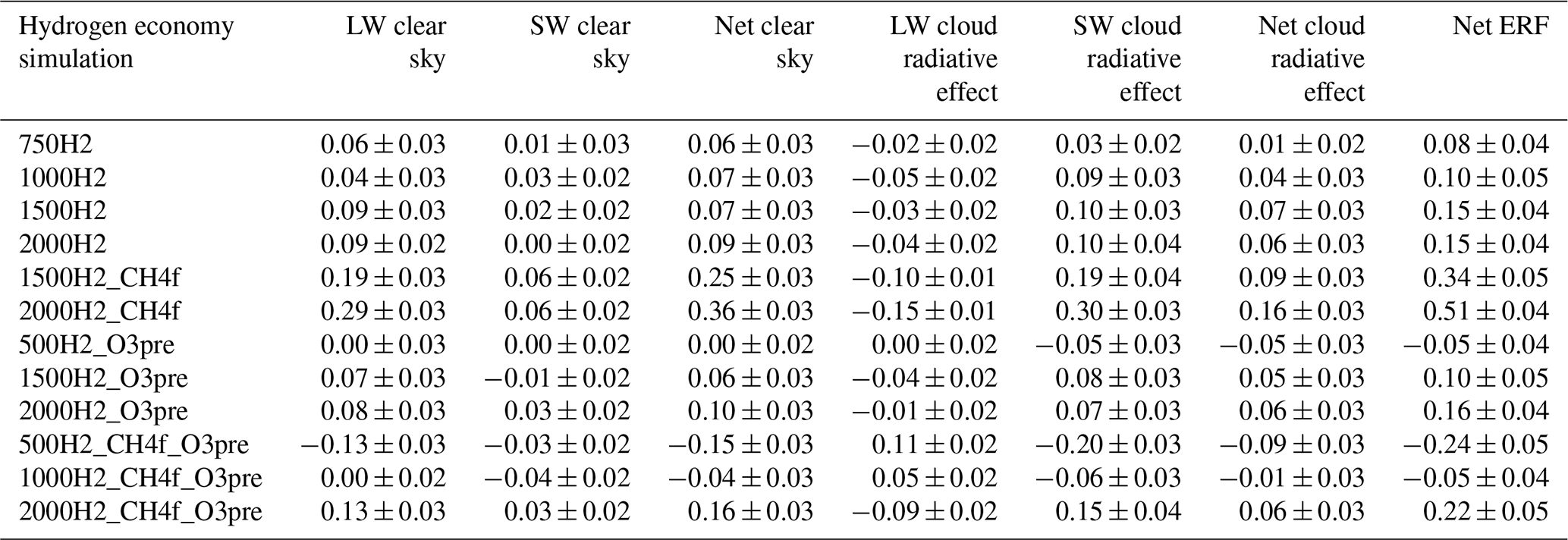
Table 2ERFs and their clear-sky and cloud radiative effect components in the shortwave (SW) and longwave (LW) calculated using the method outlined in Ghan (2013, as used in O'Connor et al., 2021, 2022), based on the last 30 years of hydrogen simulations. All units are in watts per square metre (W m−2).
3.3 Effective radiative forcing
Figure 3 shows the effective radiative forcing (ERF) for the scenarios in Table 1. Our ERF values are based on the chemical changes in composition resulting from increases in atmospheric H2, in addition to changes in emissions of CH4, CO, NOx and VOCs in the scenarios where these are included. The calculated ERFs do not include the large climate benefit expected from anticipated reductions in CO2 emissions. We determined the ERF following Eq. (8) from O'Connor et al. (2021). The ERF can also be decomposed into a clear-sky and a cloud radiative forcing, with the latter calculated from a change in the cloud radiative effect (CRE) from “clean” radiation calls that exclude aerosol–radiation interactions (Ghan, 2013). The clear-sky forcing, in principle, may include a contribution from aerosol–radiation interactions, but the magnitude of this contribution was found to be less than 0.02 W m−2. The time-slice experiments using an atmosphere-only model, i.e. using decoupled sea surface temperature (SST) and sea-ice coverage, permit the determination of the top-of-atmosphere radiative forcing including rapid adjustments to cloud and water vapour. The ERF was calculated relative to the 2014 base case. The ERF varies from a cooling (negative ERF) to a warming (positive ERF) tendency, depending on the scenario. The ERF increases with H2 over the range 500–2000 ppb. Table 2 shows that these increases are due to both clear-sky and cloud radiative forcing. The clear-sky forcing increases with increasing H2, presumably due to the increased O3, while the CRE can be ascribed to small decreases in cloud albedo. Figure 4 shows that increasing H2 from 500 to 2000 ppb leads to changes in cloud droplet number concentration (CDNC) across the globe. The decreased CDNC leads, for the same amount of water vapour, to larger cloud droplets and lower cloud albedo. This leads to a CRE of 0.05 W m−2. In scenarios where CH4 is increased, the further suppression of OH leads to a stronger CRE whilst the radiative forcing from the CRE in our hydrogen economy scenarios increases the total ERFs by approximately 50 %, thus forming a significant component of indirect forcing from H2. We do not include forcing from clouds in our GWP calculations. Such couplings between oxidants, aerosols and clouds are relatively unique in the UKESM1 compared with other CMIP6 models, and more studies are required to constrain the uncertainties involved.
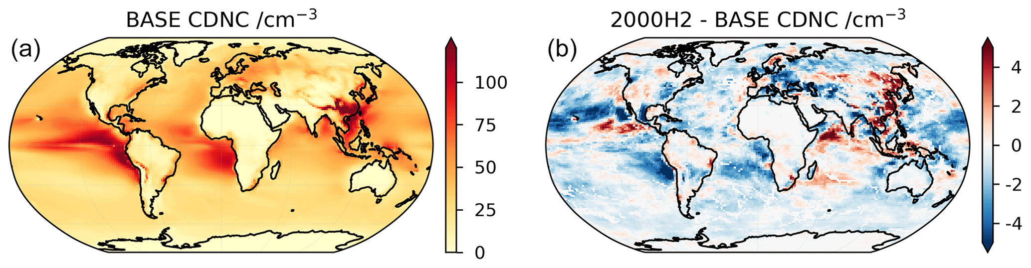
Figure 4Cloud droplet number concentration (CDNC) in the UKESM1 model at 1 km altitude. Panel (a) shows CDNC in the BASE (500 ppb H2) scenario, panel (b) the change in CDNC when H2 is increased to 2000 ppb (2000H2 scenario).
3.4 Global warming potential
A GWP quantifying the indirect radiative forcings associated with H2 has, so far, only been determined in a limited number of studies previously, including studies by Derwent et al. (2001, 2020, an update on Derwent et al., 2006), Field and Derwent (2021), Hauglustaine et al. (2022), and Sand et al. (2023). The first two studies considered only the influence of H2 on tropospheric composition, whereas Hauglustaine et al. (2022) and Sand et al. (2023) included both the tropospheric and stratospheric response. In addition to these studies, Ocko and Hamburg (2022) extended the work presented in Warwick et al. (2022), to calculate hydrogen's GWP for a range of time horizons.
We determine a GWP for H2 based on composition changes in both the troposphere and stratosphere in our UKESM1 simulations, using radiative forcing scaling factors from Myhre et al. (2013), Forster et al. (2021) and Eqs. (1) to (4) presented in Sect. 3.4.1 (see also Warwick et al., 2022). Our new estimate of the H2 GWP considers changes in methane and ozone in the troposphere and changes in stratospheric water vapour and stratospheric ozone. Note that we have not used the model-derived ERFs from Sect. 3.3 in the GWP calculations below. The model-derived ERFs (for H2 leakage only, including the methane response) are larger than the radiative forcing due to hydrogen determined from modelled changes in chemical composition using radiative forcing scaling factors from Forster et al. (2021) (see Sect. 3.4.2). Much of this difference arises due to the large contribution from clouds to the model-based ERFs (see Table 2) that is not accounted for in the radiative forcing scaling factors. For our GWP calculations, we determine the radiative forcing using the modelled changes in composition along with the radiative forcing scaling factors rather than the ERFs. Our reason for this is two-fold. Firstly, it ensures the large uncertainty associated with the aerosol–cloud component of the ERFs (Forster et al., 2021) is not propagated into the GWP calculations. Secondly, significant further work would be required to attribute the calculated total ERFs to individual species so that the appropriate lifetimes could be applied to the different components of the forcing that contribute to the GWP. However, we note that if the model ERFs were to be used in the GWP calculations, the GWPs presented in the next section would be larger.
3.4.1 Methodology
For our GWP calculation, we derive a more universal version of the approach presented by Fuglestvedt et al. (2010) for calculating GWPs for species whose emissions result in indirect radiative forcings, which was also implicitly adopted for global temperature change potentials in the IPCC Sixth Assessment Report (Forster et al., 2021). The method of Fuglestvedt et al. (2010) assumes that the time evolution of the radiative forcing depends only on the lifetime of the species causing the forcing and not the lifetime of the species being emitted. In their method, the time evolution of the radiative forcing during a 1-year constant emission is described by an approach to a steady state with a time constant according to the lifetime of the species causing the forcing. The peak forcing is assumed to occur directly at the end of the 1-year emission and to subsequently decay with the same lifetime as in the growth phase. Although this assumption may be a good approximation for short-lived emission species such as NOx, it may not be for species with longer lifetimes such as H2. Our extension of their method (see Warwick et al., 2022) accounts for both the lifetime of the emitted species and the lifetime of the species causing the forcing, as well as allowing the time period of the constant emission to be varied. The use of a 1-year constant emission rather than an emission pulse has the benefit of removing the time-of-year dependence for when the emission pulse occurs.
In our method for deriving indirect GWPs from steady-state simulations, we include the indirect forcing due to perturbations in radiatively active species arising (a) during the constant emission (AGWP1, Eq. 1), (b) from the decay of the perturbation subsequent to the end of the constant emission (AGWP2, Eq. 2) and (c) from perturbations arising from the emission species remaining in the atmosphere after the end of the constant emission (AGWP, Eq. 3). Derivations for Eqs. (1) to (3) are presented in the Supplement.
where AGWP is the absolute global warming potential (W m−2 kg−1 yr); M is the species resulting in the indirect radiative forcing, CH4, O3 and H2O (ppb or DU for tropospheric O3); RM is the radiative forcing efficiency for M (W m−2 ppb−1 or W m−2 DU−1 for tropospheric O3); aM is the production rate of M (ppb yr−1) per ppb H2 change at the steady state (yr−1); αM is the atmospheric lifetime of M (years); αH is the atmospheric H2 lifetime (combined chemical and deposition lifetime) (years); Hz is the time horizon considered (years); C is the conversion factor for converting H2 mixing ratio (ppb) into H2 mass (kg) and tp is the length of step emission (years).
Equations (1) to (3) are applied separately to methane, non-methane-induced ozone and stratospheric water vapour to calculate a net GWP for H2. The associated indirect GWPs for each radiative species perturbed by hydrogen are then given by
A comparison of the time evolution of the methane perturbation resulting from a change in H2 mixing ratio based on the standard (Fuglestvedt et al. 2010) equations and Fig. 5 shows our updated equations. Accounting for the atmospheric lifetime of hydrogen in the updated equations results in a slower predicted rate of increase in methane during the 1-year constant emission relative to the standard (Fuglestvedt et al. 2010) equations, a delayed methane peak (peaking at 5 years rather than 1 year, using the parameters specified in the caption) and a slower rate of methane decrease subsequent to that peak, as methane is still being impacted by the remaining H2. This difference occurs because the equations of Fuglestvedt et al. (2010) assume that the emitted species instantaneously reaches a new steady-state atmospheric concentration at the start of the 1-year constant emission. In addition, their assumption that the decay following the peak forcing is controlled only by the lifetime of the radiatively active species neglects any subsequent perturbations to atmospheric chemistry as a result of the emitted species still present in the atmosphere after the end of the 1-year constant emission. A comparison of the transient methane growth due to a H2 perturbation, as determined by Eqs. (1) to (3) in Fig. 5 (grey line), with model studies where methane has been free to respond to a H2 perturbation (including the box model described in Sect. 2.2 and the model studies of Derwent et al., 2020, and Bertagni et al., 2022) shows that the response represented by Eqs. (1) to (3) is similar to that found in transient model simulations following a H2 pulse emission.
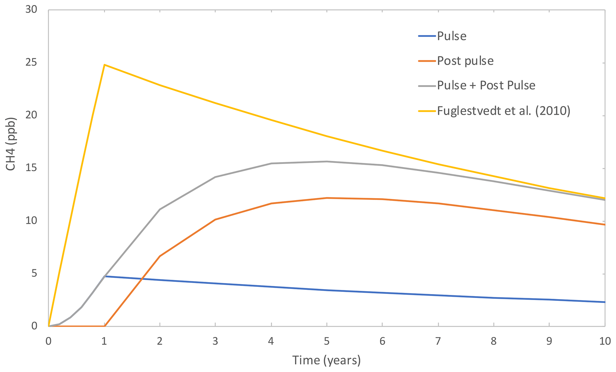
Figure 5The time evolution of excess methane during and after a 1-year step hydrogen emission (based on a steady-state H2 excess of +1500 ppb, an H2 lifetime of 1.96 years and a methane perturbation lifetime of 11.8 years) as predicted by the equations of Fuglestvedt et al. (2010) (yellow) and our updated equations. For our updated equations, the excess methane is split into contributions from methane generated during the step emission (blue), methane generated from excess hydrogen remaining in the atmosphere after the 1-year step emission (orange). The total methane excess in shown in grey.
Equations (1) to (3) are obtained using a framework assuming a 1-year constant emission rather than an emission pulse. This has the benefit of removing the time-of-year dependence of the atmospheric perturbations arising from the emission pulse. However, once obtained, the chemical parameters from our UKESM1 simulations can also be applied to the pure pulse approach with little error. Equations (1) to (3) can be simplified by using the tp→0 limit of Eq. (2), which is given in Eq. (5). Based on our obtained parameters, using Eq. (5) rather than Eqs. (1) to (3) leads to a difference of 0.1 % for our hydrogen GWP(100) and 1.5 % for our hydrogen GWP(20). In contrast, using the original method of Fuglestvedt et al. (2010) leads to a 0.1 % difference in our hydrogen GWP(100) but a 5 % difference in our hydrogen GWP(20) relative to Eqs. (1) to (3).
3.4.2 Calculation of a hydrogen GWP
In our calculations, AGWP(100) and AGWP(20) are taken to be 9.17 × 10⁻¹⁴ (± 26 %) and 2.49 × 10⁻¹⁴ (± 18 %) W m−2 kg−1 yr (Myhre et al., 2013) respectively. AGWP is taken as the sum of AGWP1–3. The values for AGWP(100) and AGWP(20) change slightly to 8.95 × 10⁻¹⁴ (± 26 %) and 2.43 × 10⁻¹⁴ (± 18 %) W m−2 kg−1 yr respectively in Forster et al. (2021). Table 3 shows the impact of this on our H2 GWP calculation, along with other IPCC AR6 (Forster et al., 2021) updates. The length of the step emission, tp, is 1 year, Hz is taken to be 20 or 100 years, and aH is 1.96 years (with an uncertainty range from 1.4 to 2.2 years). The conversion factor, C, for converting H2 mixing ratio into H2 mass based on the UKESM1 data is 3.52 × 10⁻⁹ ppb kg−1. Values for RM, aM and αM are dependent on the species causing the indirect forcing (methane, ozone and stratospheric water vapour).
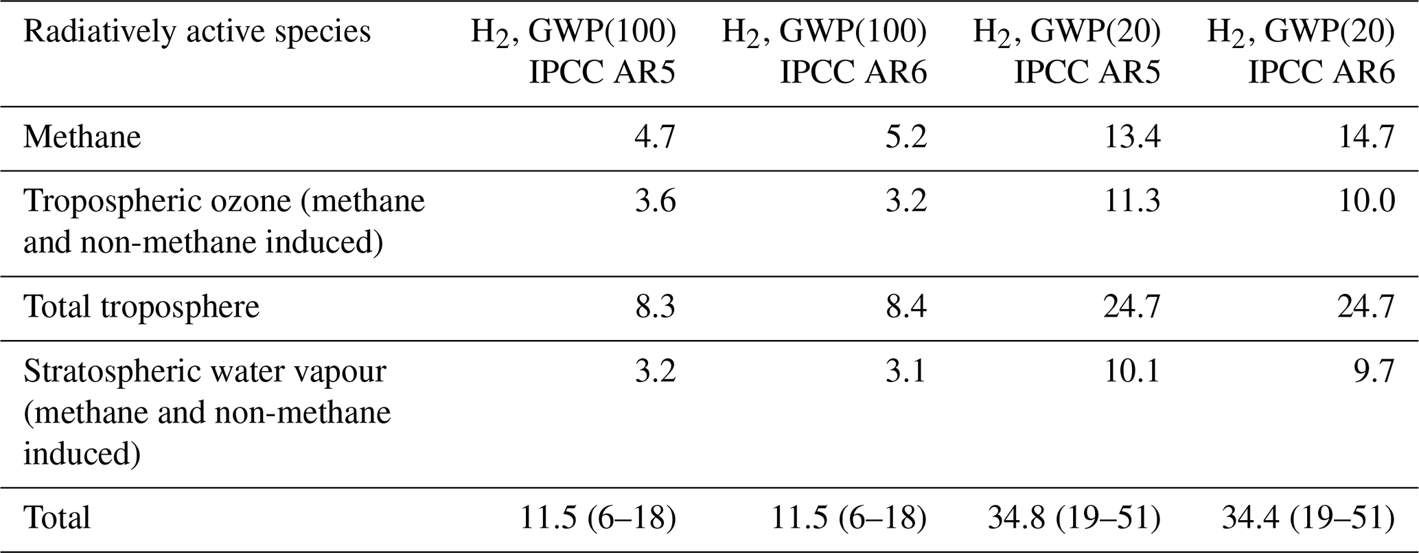
Table 3A comparison of the 100- and 20-year time horizon H2 GWPs (GWP(100) and GWP(20) respectively) determined using radiative efficiencies and the AGWP for CO2 from IPCC AR5 (Myhre et al., 2013) and from IPCC AR6 (Forster et al., 2021). The uncertainties quoted account for uncertainties in the H2 lifetime with respect to soil uptake, radiative forcing scaling factors and the AGWP only.
For methane, is taken to be 0.000363 (± 10 %) W m−2 (ppb CH4)−1 (Myhre et al., 2013) or 0.000389 W m−2 (ppb CH4)−1 (Forster et al., 2021). The methane perturbation lifetime, , in UKESM1 is determined to be 11.8 years in this study, which falls within the range given by IPCC AR5 (12.4 ± 1.4 years, Myhre et al., 2013). The value for , an additional methane production rate term per unit increase in H2, represents the positive CH4 tendency resulting from an increase in H2 and corresponding decrease in OH and is defined as
where CH4 is the methane lower boundary condition (1835 ppb in UKCA), is the global mean air-mass-weighted rate constant for the reaction of CH4 with OH and is the rate of change in air-mass-weighted tropospheric mean OH with respect to H2. Values for these parameters derived from UKESM1 simulations are as follows: k(CH4+OH) = 2.8 × 10⁻¹⁵ cm3 molec.−1 s−1 and = 3.68 × 10⁻⁹ (dimensionless). k(CH4+OH) is determined from the gradient of methane lifetime against 1 (global air-mass-weighted mean OH) and from the gradient of the mass-weighted tropospheric mean OH concentration against H2 surface mixing ratio for the UKESM1 simulations including the feedback on the methane lifetime via an adjusted CH4 lower boundary condition determined by the box model (see Fig. 1a). Note that if we weight OH by reaction with CH4 instead of air mass, the value determined for k(CH4+OH) halves (1.4 × 10⁻¹⁵ cm3 molec.−1 s−1), the value for doubles (7.36 × 10⁻⁹ (dimensionless)) and our value for remains unaltered. It is also possible to derive using the gradient of the mass-weighted tropospheric mean OH concentration against H2 surface mixing ratio from the UKESM1 simulations where only the H2 LBC is varied (whilst the CH4 LBC is held constant), in combination with the equation below from Stevenson et al. (2013), and the methane feedback factor of 1.39 derived for UKESM1,
where f is the methane feedback factor, CH4 base and τbase are the lower boundary condition and methane lifetime in the base scenario, and CH4 new and τnew are the lower boundary condition and methane lifetime in the perturbed H2 scenario. The difference between the values obtained using the two methods above is approximately 3 %. This, in turn, leads to a 3 % difference in the methane-induced hydrogen GWP terms and a difference of less than 1 % in the total hydrogen GWP when accounting for all forcings. This difference is negligible in comparison to other uncertainties (see Table 3); therefore our GWP calculation remains independent of the box model results.
The indirect forcing from methane-induced changes in tropospheric ozone and stratospheric water vapour are determined by multiplying the calculated direct methane forcing () by scaling factors of 0.5 ± 55 % and 0.15 ± 70 % respectively (Myhre et al., 2013). Equivalent scaling factors, from Forster et al. (2021), are 0.37 ± 50 % and 0.106 ± 100 %.
In addition to the methane-induced indirect radiative forcing from ozone and water vapour outlined above, we also consider non-methane-induced radiative forcing from H2 as a source of tropospheric ozone and stratospheric water vapour. For stratospheric water vapour, the e-folding lifetime of the water vapour perturbation following a change in H2, , is derived from model spin-up data following a change in the H2 lower boundary condition and is determined to be 8 years in the lower stratosphere. Values for both and are determined by the steady-state change in the stratospheric water profile between our UKESM1 BASE simulation and the simulation where the H2 lower boundary condition is increased from 500 to 2000 ppb. A comparison of the vertical profile of stratospheric water vapour changes resulting from H2 changes in our study (Fig. 1d), with that resulting from methane changes between 1950 and 2000 in Fig. 2b of Myhre et al. (2007), shows very similar H2O changes at all altitudes. We therefore adopt the radiative forcing determined by Myhre et al. (2007) of 0.05 W m−2 with an estimated uncertainty of ±20 % for stratospheric water vapour changes relative to base in our 2000H2 UKESM1 scenario. This water vapour forcing is associated with a change of ∼ 500 ppb in stratospheric water vapour at 30 km altitude, giving a value for of 1 × 10⁻⁴ W m−2 (ppb H2O)−1 when considering changes at 30 km. We assume that the entire stratospheric H2O profile will scale proportionally with the H2 lower boundary condition (following results from our UKESM1 simulations using H2 LBCs of 750, 1000, 1500 and 2000 ppb H2), so the choice of 30 km for determining is arbitrary. The production rate of water vapour per ppb change in H2, , can then be defined as the change in steady-state H2O at 30 km (500 ppb) divided by the lifetime of 8 years and the change in H2 mixing ratio of 1500 ppb.
For changes in the global mean tropospheric ozone column, the value for is 0.042 (0.037 to 0.047) W m−2 DU−1 and is taken directly from Myhre et al. (2013). No updated value for was presented by Forster et al. (2021), although a similar value of 0.039 W m−2 DU−1 can be obtained based on the estimated change in tropospheric ozone of 109 ± 25 Tg between 1850 and 2005 and a stratospheric-temperature-adjusted radiative forcing due to tropospheric ozone of 0.39 ± 0.07 W m−2 between 1850 and 2010. The e-folding lifetime associated with the ozone perturbation, , is taken to be 0.07 years, calculated as the tropospheric O3 burden divided by the loss in our UKESM1 base simulation. This is shorter than the lifetime used for the short-lived ozone perturbation by Fuglestvedt et al. (2010) of 0.267 years. However, our results are insensitive to the difference between these values and small variations around them. The value for is calculated as the change in the steady-state global mean tropospheric ozone column in our 2000H2 simulation relative to base (0.59 DU) divided by the lifetime of 0.07 years and the change in H2 mixing ratio of 1500 ppb. A list of all the input parameters, with the values used in our AGWP calculations, is presented in Table S1. Changes in the H2 mixing ratio can also influence stratospheric ozone. In our UKESM1 simulations, the change in global mean stratospheric ozone column between our base and 2000H2_CH4f (increased H2, including the chemical feedback on the methane lifetime) scenarios was negligible at +0.10 DU, relative to a base value of 283.78 DU and interannual variations of up to several DU. Based on a value of R for stratospheric ozone of 0.0054 W m−2 DU−1 (Schwarzkopf and Ramaswamy, 1993) and a range of e-folding lifetimes for the stratospheric ozone perturbation of between 1 and 10 years, the results obtained are a GWP(100) of less than 0.03 using Eqs. (1) to (4). We consider this to be below the uncertainty involved in the calculation and conclude that changes in stratospheric ozone for our range of scenarios do not significantly contribute to the hydrogen GWP.
For a 100-year time horizon we determine a H2 GWP of 12 ± 6 (see Table 3). This value is larger than previously published studies, which do not account for changes in stratospheric composition (Derwent et al., 2020, 5 ± 1, and Field and Derwent, 2021, 3.3 ± 1.4), but similar to the values of Hauglustaine et al. (2022) (12.8 ± 5.2) and the multimodel study of Sand et al. (2023) (11.6 ± 2.8, 1 standard deviation), which include a tropospheric and stratospheric response. Approximately two-thirds of our GWP arise from the influence of H2 on methane and ozone distributions in the troposphere, and one-third arises from the influence of H2 on stratospheric water vapour. Results from our study can also be compared with that of Paulot et al. (2021), who estimated the indirect radiative forcing at a steady state due to an increase in H2. Their study accounted for changes in methane, tropospheric ozone and stratospheric water vapour and found an indirect radiative forcing arising from a H2 of 0.13 mW m−2 (ppb H2)−1. Using the radiative forcing scaling factors, we obtain a larger value of 0.18 ± 0.03 mW m−2 (ppb H2)−1 (the same value is obtained using both the Myhre et al., 2013, and Forster et al., 2021, radiative efficiency scaling factors), which may partly be explained by the larger methane feedback factor in UKESM1 (1.39) relative to the chemistry–climate model used in (Paulot et al., 2021).
Uncertainties in our calculation are based on uncertainties in the hydrogen lifetime with respect to soil uptake, uncertainties in radiative forcing scaling factors and the AGWP for CO2. We do not account for uncertainties in chemical lifetimes and other UKESM1-derived quantities which are likely to vary when using different atmospheric models with different chemistry schemes. In addition, we also note that the sensitivity of ERF in UKESM1 to changes in methane is approximately 65 % larger than that indicated by the radiative scaling factors used in the empirical relationships applied in the GWP calculation (O'Connor et al., 2022). This suggests a further source of uncertainty than accounted for by the radiative forcing scaling factor uncertainties outlined by Myhre et al. (2013) and Forster et al. (2021), associated with the response of aerosols, clouds, ozone and water vapour to changing methane levels.
The leakage of hydrogen associated with a hydrogen economy will result in indirect global warming, offsetting greenhouse gas emission reductions made as a result of a switch from fossil fuel to hydrogen. We have presented a methodology for calculating the indirect GWP of H2, with principal contributions coming from changes in methane, tropospheric ozone and stratospheric water vapour. The GWP depends on the lifetime of H2 in the atmosphere, the perturbation lifetimes of the radiatively active species (e.g. CH4 and O3) and their effective production rates per unit change in H2. We present values for these based on calculations with our chemistry–climate model, UKESM1 and a box model. The 100-year GWP for H2, based on the above, is 12 ± 6, a value somewhat higher than some previous estimates but similar to recent values from Hauglustaine et al. (2022) and Sand et al. (2023). Whilst our GWP uncertainty accounts for uncertainties associated with the size of the soil sink and radiative forcing scaling factors, it does not include uncertainties in model-derived parameters (e.g. chemical and perturbation lifetimes or the chemical production rates per unit change in H2). In particular, uncertainties associated with the stratospheric response may be significant, as well as the response of aerosols and clouds to changing methane levels. Further simulations using different Earth system models and different chemistry schemes would be required to fully assess the impact of uncertainties in these parameters on the hydrogen GWP.
Determining a GWP for hydrogen allows a change in hydrogen emissions to be compared to an equivalent change in carbon dioxide emissions in terms of time-integrated radiative forcing. This increase in equivalent carbon dioxide emissions can be compared with expected reductions in carbon dioxide and methane (as equivalent CO2) emissions to determine the net impact on radiative forcing. In our illustrative future global hydrogen economy scenario (Sect. 2.3), we estimate additional H2 emissions of between 9 and 95 Tg H2 yr−1, based on a hydrogen economy supplying 23 % of present-day energy consumption and H2 leakage rates of 1 % and 10 %. Using a H2 GWP(100) of 12, this is equivalent to the time-integrated radiative forcing from carbon dioxide emissions of about 110 and 1140 Tg CO2 yr−1 respectively. Based on the fossil fuel energy sectors that are replaced by hydrogen, a low-carbon method of hydrogen generation and the sector emissions described in Hoesly et al. (2018), we would expect a reduction in carbon dioxide emissions of ∼ 26 000 Tg yr−1. In addition, a further reduction of ∼ 1200 Tg yr−1 equivalent CO2 emissions would result from expected methane emission reductions (assuming a GWP(100) for methane of 28), resulting in a total reduction of CO2 equivalent emissions of ∼ 27 200 Tg yr−1. Therefore, in this global scenario the increase in equivalent CO2 emissions, based on 1 % and 10 % H2 leakage rates, offsets approximately 0.4 % and 4 % of the total equivalent CO2 emission reductions respectively. Whilst the benefits from equivalent CO2 emission reductions significantly outweigh the disbenefits arising from H2 leakage, they clearly demonstrate the climate importance of controlling H2 leakage within a hydrogen economy.
A switch to a hydrogen economy would also provide the opportunity to reduce emissions of other gases, which can themselves directly or indirectly affect both climate and air quality. For example, an immediate impact of increased atmospheric H2 is the reduction of the concentration of OH, the major tropospheric oxidant, which would thus tend to increase the lifetime of methane. Increases in methane would adversely affect climate and also lead to production of tropospheric ozone, impacting both climate and air quality. However, we show that reductions in methane emissions associated with decreased fossil fuel use, along with reductions of CO and NOx emissions, could lead to a net change in ozone close to (or below) zero with associated climate and air quality benefits, assuming very high H2 leakage rates (e.g. scenario 2000H2_CH4f_O3pre, Fig. 2j) and a green method of hydrogen production. In the case of no leakage of H2, emission reductions in methane, CO and NOx lead to decreases in tropospheric ozone column globally (scenario 500H2, CH4f_O3pre, Fig. 2h). To assess whether the ozone response to changes in emissions associated with a hydrogen economy is influenced by the assumed background climate conditions (i.e. whether the timing of the implementation of a hydrogen economy could be important), we performed a set of additional model simulations using 2045–2055 climatological boundary conditions taken from the CMIP6–SSP2-4.5 scenario. These scenarios assumed a hydrogen economy of the same absolute size and identical leakage rates to our present-day (2014) scenarios. We found no discernible difference between the tropospheric and stratospheric ozone response to changes in H2 and ozone precursors. Emission reductions, from decreased fossil fuel use, offer similar air-quality benefits in both sets of simulations. To maximise the benefit of a switch to hydrogen, not only should hydrogen leakage be minimised, but the emissions of methane, CO, VOCs and NOx should also be reduced to the maximum extent possible.
Due to intellectual property rights restrictions, we cannot provide either the source code or documentation papers for the UM. The Met Office Unified Model is available for use under licence. A number of research organisations and national meteorological services use the UM in collaboration with the Met Office to undertake basic atmospheric process research, produce forecasts, develop the UM code, and build and evaluate Earth system models. For further information on how to apply for a licence, see http://www.metoffice.gov.uk/research/modelling-systems/unified-model (last access: October 2023).
CMIP6 data used in this study are available through the Earth System Grid Federation (ESGF; https://esgf-index1.ceda.ac.uk/projects/cmip6-ceda/, last access: October 2023; https://doi.org/10.22033/ESGF/CMIP6.4497, Bader et al., 2019a; https://doi.org/10.22033/ESGF/CMIP6.11485, Bader et al., 2019b).
The supplement related to this article is available online at: https://doi.org/10.5194/acp-23-13451-2023-supplement.
JAP and ATA designed the research and supervised the analysis. JK performed the UKESM1 model simulations and atmospheric composition analysis and PTG and FMO'C performed the ERF calculations. KPS, JAP, PTG and NJW contributed to the H2 GWP analysis. KPS derived the AGWP equations, with contributions from JAP. NJW performed the UKESM1 GWP calculations. All box modelling was performed by PTG. NJW compiled the emission changes in the different scenarios. All authors contributed to the writing of this paper.
The contact author has declared that none of the authors has any competing interests.
Publisher's note: Copernicus Publications remains neutral with regard to jurisdictional claims made in the text, published maps, institutional affiliations, or any other geographical representation in this paper. While Copernicus Publications makes every effort to include appropriate place names, the final responsibility lies with the authors.
Model simulations and analysis were performed using Monsoon2, a collaborative high-performance computing facility funded by the Met Office and the Natural Environment Research Council; JASMIN, the UK collaborative data analysis facility; and the NEXCS High Performance Computing facility funded by the Natural Environment Research Council and delivered by the Met Office. We thank Ken Caldeira and Lei Duan, Carnegie Institution for Science, for their contribution to the derivation of the AGWP equations. We also thank two reviewers, Matteo Bertagni, Princeton University, and Bill Collins, University of Reading, for useful comments that have helped improve the manuscript.
This research has been supported by the Department for Business, Energy and Industrial Strategy, UK Government (grant no. CR19062). In addition, the HECTER project supported Alex T. Archibald, Paul T. Griffiths, Nicola J. Warwick (NE/X010236/1) and Keith P. Shine (NE/X010732/1) in the latter stages of this work. Fiona M. O'Connor was supported by the Met Office Hadley Centre Climate Programme, funded by BEIS.
This paper was edited by Chul Han Song and reviewed by two anonymous referees.
Alvarez, R. A., Zavala-Araiza, D., Lyon, D. R., Allen, D. T., Barkley, Z. R., Brandt, A. R., Davis, K. J., Herndon, S. C., Jacob, D. J., Karion, A., and Kort, E. A.: Assessment of methane emissions from the US oil and gas supply chain, Science, 361, 186–188, 2018.
Archibald, A. T., Neu, J. L., Elshorbany, Y. F., Cooper, O. R., Young, P.J., Akiyoshi, H., Cox, R. A., Coyle, M., Derwent, R. G., Deushi, M., Finco, A., Frost, G. J., Galbally, I. E., Gerosa, G., Granier, C., Griffiths, P. T., Hossaini, R., Hu, L., Jöckel, P., Josse, B., Lin, M. Y., Mertens, M., Morgenstern, O., Naja, M., Naik, V., Oltmans, S., Plummer, D. A., Revell, L. E., Saiz-Lopez, A., Saxena, P., Shin, Y. M., Shahid, I., Shallcross, D., Tilmes, S., Trickl, T., Wallington, T. J., Wang, T., Worden, H. M., and Zeng, G.: Tropospheric Ozone Assessment Report: A critical review of changes in the tropospheric ozone burden and budget from 1850 to 2100, Elem. Sci. Anth., 8, 034, https://doi.org/10.1525/elementa.2020.034, 2020a.
Archibald, A. T., O'Connor, F. M., Abraham, N. L., Archer-Nicholls, S., Chipperfield, M. P., Dalvi, M., Folberth, G. A., Dennison, F., Dhomse, S. S., Griffiths, P. T., Hardacre, C., Hewitt, A. J., Hill, R. S., Johnson, C. E., Keeble, J., Köhler, M. O., Morgenstern, O., Mulcahy, J. P., Ordóñez, C., Pope, R. J., Rumbold, S. T., Russo, M. R., Savage, N. H., Sellar, A., Stringer, M., Turnock, S. T., Wild, O., and Zeng, G.: Description and evaluation of the UKCA stratosphere–troposphere chemistry scheme (StratTrop vn 1.0) implemented in UKESM1, Geosci. Model Dev., 13, 1223–1266, https://doi.org/10.5194/gmd-13-1223-2020, 2020b.
Bader, D. C., Leung, R., Taylor, M., and McCoy, R. B.: E3SMProject E3SM1.0 model output prepared for CMIP6 CMIP historical, Version 20201101, Earth System Grid Federation [data set], https://doi.org/10.22033/ESGF/CMIP6.4497, 2019a.
Bader, D. C., Leung, R., Taylor, M., and McCoy, R. B.: E3SMProject E3SM1.1 model output prepared for CMIP6 CMIP historical, Version 20201101, Earth System Grid Federation [data set], https://doi.org/10.22033/ESGF/CMIP6.11485, 2019b.
Bertagni, M. B., Pacala, S. W., Paulot, F., and Porporaro, A.: Risk of the hydrogen economy for atmospheric methane, Nat. Comm., 13, 7706, https://doi.org/10.1038/s41467-022-35419-7, 2022.
BP: Energy Outlook, 2020 Edition, https://www.bp.com/content/dam/bp/business-sites/en/global/corporate/pdfs/energy-economics/energy-outlook/bp-energy-outlook-2020.pdf (last access: October 2023), 2020.
Derwent, R., Simmonds, P., O'Doherty, S., Manning, A., Collins, W., and Stevenson, D.: Global environmental impacts of the hydrogen economy, International Journal of Nuclear Hydrogen Production and Applications, 1, 57–67, 2006.
Derwent, R. G., Collins, W. J., Johnson, C. E., and Stevenson, D. S.: Transient behaviour of tropospheric ozone precursors in a global 3D CTM and their indirect greenhouse effects, Climatic Change, 49, 463–487, 2001.
Derwent, R. G., Stevenson, D. S., Utembe, S. R., Jenkin, M. E., Khan, A. H., and Shallcross, D. E.: Global modelling studies of hydrogen and its isotopomers using STOCHEM-CRI: Likely radiative forcing consequences of a future hydrogen economy, Int. J. Hydrogen Energ., 45, 9211–9221, 2020.
E4tech, Ltd: H2 emission potential review, Department for Business, Energy and Industrial Strategy, BEIS Research Paper Number 22, https://assets.publishing.service.gov.uk/media/5cc6f1e640f0b676825093fb/H2_Emission_Potential_Report_BEIS_E4tech.pdf (last access: October 2023), 2019.
Ehhalt, D. H. and Rohrer, F.: The tropospheric cycle of H2: a critical review, Tellus B, 61, 500–535, 2009.
Field, R. A. and Derwent, R.: Global warming consequences of replacing natural gas with hydrogen in the domestic energy sectors of future low-carbon economies in the United Kingdom and the United States of America, Int. J. Hydrogen Energ., 46, 30190–30203, https://doi.org/10.1016/j.ijhydene.2021.06.120, 2021.
Forster, P., Storelvmo, T., Armour, K., Collins, W., Dufresne, J.-L., Frame, D., Lunt, D. J., Mauritsen, T., Palmer, M. D., Watanabe, M., Wild, M., and Zhang, H.: The Earth's Energy Budget, Climate Feedbacks, and Climate Sensitivity, in: Climate Change 2021: The Physical Science Basis. Contribution of Working Group I to the Sixth Assessment Report of the Intergovernmental Panel on Climate Change, edited by: Masson-Delmotte, V., Zhai, P., Pirani, A., Connors, S. L., Péan, C., Berger, S., Caud, N., Chen, Y., Goldfarb, L., Gomis, M. I., Huang, M., Leitzell, K., Lonnoy, E., Matthews, J. B. R., Maycock, T. K., Waterfield, T., Yelekçi, O., Yu, R., and Zhou, B., Cambridge University Press, Cambridge, United Kingdom and New York, NY, USA, 923–1054, https://doi.org/10.1017/9781009157896.009, 2021.
Frazer-Nash Consultancy: Fugitive hydrogen emissions in a future hydrogen economy, research paper for BEIS, Department for Business, Energy and Industrial Strategy, https://www.gov.uk/government/publications/fugitive-hydrogen-emissions-in-a-future-hydrogen-economy (last access: October 2023), 2022.
Fuglestvedt, J. S., Shine, K. P., Berntsen, T., Cook, J., Lee, D. S., Stenke, A., Skeie, R. B., Velders, G. J. M., and Waitz, I. A.: Transport impacts on atmosphere and climate: Metrics, Atmos. Environ., 44, 4648–4677, 2010.
Ghan, S. J.: Technical Note: Estimating aerosol effects on cloud radiative forcing, Atmos. Chem. Phys., 13, 9971–9974, https://doi.org/10.5194/acp-13-9971-2013, 2013.
Gidden, M. J., Riahi, K., Smith, S. J., Fujimori, S., Luderer, G., Kriegler, E., van Vuuren, D. P., van den Berg, M., Feng, L., Klein, D., Calvin, K., Doelman, J. C., Frank, S., Fricko, O., Harmsen, M., Hasegawa, T., Havlik, P., Hilaire, J., Hoesly, R., Horing, J., Popp, A., Stehfest, E., and Takahashi, K.: Global emissions pathways under different socioeconomic scenarios for use in CMIP6: a dataset of harmonized emissions trajectories through the end of the century, Geosci. Model Dev., 12, 1443–1475, https://doi.org/10.5194/gmd-12-1443-2019, 2019.
Grant, A., Archibald, A. T., Cooke, M. C., Nickless, G., and Shallcross, D. E.: Modelling the oxidation of 15 VOCs to track yields of hydrogen, Atmos. Sci. Lett., 11, 265–269, 2010.
Hauglustaine, D., Paulot, F., Collins, W. Derwent, R., Sand, M., and Boucher, O.: Climate benefit of a future hydrogen economy, Commun. Earth Environ., 3, 295, https://doi.org/10.1038/s43247-022-00626-z, 2022.
Heimann, I., Griffiths, P. T., Warwick, N. J., Abraham, N. L., Archibald, A. T., and Pyle, J. A.: Methane emissions in a chemistry-climate model: Feedbacks and climate response, J. Adv. Model. Earth Sys., 12, e2019MS002019, https://doi.org/10.1029/2019MS002019, 2020.
Hoesly, R. M., Smith, S. J., Feng, L., Klimont, Z., Janssens-Maenhout, G., Pitkanen, T., Seibert, J. J., Vu, L., Andres, R. J., Bolt, R. M., Bond, T. C., Dawidowski, L., Kholod, N., Kurokawa, J.-I., Li, M., Liu, L., Lu, Z., Moura, M. C. P., O'Rourke, P. R., and Zhang, Q.: Historical (1750–2014) anthropogenic emissions of reactive gases and aerosols from the Community Emissions Data System (CEDS), Geosci. Model Dev., 11, 369–408, https://doi.org/10.5194/gmd-11-369-2018, 2018.
Jacobson, M. Z.: Effects of wind-powered hydrogen fuel cell vehicles on stratospheric ozone and global climate, Geophys. Res. Lett., 35, L19803, https://doi.org/10.1029/2008GL035102, 2008.
Kuhlbrodt, T., Jones, C. G., Sellar, A., Storkey, D., Blockley, E., Stringer, M., Hill, R., Graham, T., Ridley, J., Blaker, A., Calvert, D., Copsey, D., Ellis, R., Hewitt, H., Hyder, P., Ineson, S., Mulcahy, J., Siahaan, A., and Walton, J.: The low-resolution version of HadGEM3 GC3.1: Development and evaluation for global climate, J. Adv. Model. Earth Sys., 10, 2865–2888, https://doi.org/10.1029/2018MS001370, 2018.
Lewis, A. C.: Optimising air quality co-benefits in a hydrogen economy: a case for hydrogen-specific standards for NOx emissions, Environmental Science: Atmospheres, 1, 201–207, 2021.
Mulcahy, J. P., Johnson, C., Jones, C. G., Povey, A. C., Scott, C. E., Sellar, A., Turnock, S. T., Woodhouse, M. T., Abraham, N. L., Andrews, M. B., Bellouin, N., Browse, J., Carslaw, K. S., Dalvi, M., Folberth, G. A., Glover, M., Grosvenor, D. P., Hardacre, C., Hill, R., Johnson, B., Jones, A., Kipling, Z., Mann, G., Mollard, J., O'Connor, F. M., Palmiéri, J., Reddington, C., Rumbold, S. T., Richardson, M., Schutgens, N. A. J., Stier, P., Stringer, M., Tang, Y., Walton, J., Woodward, S., and Yool, A.: Description and evaluation of aerosol in UKESM1 and HadGEM3-GC3.1 CMIP6 historical simulations, Geosci. Model Dev., 13, 6383–6423, https://doi.org/10.5194/gmd-13-6383-2020, 2020.
Myhre, G., Nilsen, J. S., Gulstad, L., Shine, K. P., Rognerud, B., and Isaksen, I. S. A.: Radiative forcing due to stratospheric water vapour from CH4 oxidation, Geophys. Res. Lett., 34, L01807, https://doi.org/10.1029/2006GL027472, 2007.
Myhre, G., Shindell, D., Bréon, F.-M., Collins, W., Fuglestvedt, J., Huang, J., Koch, D., Lamarque, J.-F., Lee, D., Mendoza, B., Nakajima, T., Robock, A., Stephens, G., Takemura, T., and Zhang, H.: Anthropogenic and Natural Radiative Forcing, in: Climate Change 2013: The Physical Science Basis. Contribution of Working Group I to the Fifth Assessment Report of the Intergovernmental Panel on Climate Change, edited by: Stocker, T. F., Qin, D., Plattner, G.-K., Tignor, M., Allen, S. K., Boschung, J., Nauels, A., Xia, Y., Bex, V., and Midgley, P. M., Cambridge University Press, Cambridge, United Kingdom and New York, NY, USA, https://doi.org/10.1017/CBO9781107415324, 2013.
Nisbet, E., Fisher, R., Lowry, D., France, J., Allen, G., Bakkaloglu, S., Broderick, T., Cain, M., Coleman, M., Fernandez, J., Forster, G., Griffiths, P., Iverach, C., Kelly, B., Manning, M., Nisbet-Jones, P., Pyle, J., Townsend-Small, A., Al-Shalaan, A., Warwick, N., and Zazzeri, G.: Methane mitigation: methods to reduce emissions, on the path to the Paris Agreement, Rev. Geophys., 58, e2019RG000675, https://doi.org/10.1029/2019rg000675, 2020.
Novelli, P. C., Lang, P. M., Masarie, K. A., Hurst, D. F., Myers, R., and Elkins, J. W.: Molecular hydrogen in the troposphere: Global distribution and budget, J. Geophys. Res., 104, 30427–30444, 1999.
Ocko, I. B. and Hamburg, S. P.: Climate consequences of hydrogen emissions, Atmos. Chem. Phys., 22, 9349–9368, https://doi.org/10.5194/acp-22-9349-2022, 2022.
O'Connor, F. M., Abraham, N. L., Dalvi, M., Folberth, G. A., Griffiths, P. T., Hardacre, C., Johnson, B. T., Kahana, R., Keeble, J., Kim, B., Morgenstern, O., Mulcahy, J. P., Richardson, M., Robertson, E., Seo, J., Shim, S., Teixeira, J. C., Turnock, S. T., Williams, J., Wiltshire, A. J., Woodward, S., and Zeng, G.: Assessment of pre-industrial to present-day anthropogenic climate forcing in UKESM1, Atmos. Chem. Phys., 21, 1211–1243, https://doi.org/10.5194/acp-21-1211-2021, 2021.
O'Connor, F. M., Johnson, B. T., Jamil, O., Andrews, T., Mulcahy, J. P., and Manners, J.: Apportionment of the pre-industrial to present-day climate forcing by methane using UKESM1: The role of the cloud radiative effect, J. Adv. Model. Earth Sys., 14, e2022MS002991, https://doi.org/10.1029/2022MS002991, 2022.
Patterson, J. D., Aydin, M., Crotwell, A. M., and Saltzman, E. S.: H2 in Antarctic firn air: Atmospheric reconstructions and implications for anthropogenic emissions, P. Natl. Acad. Sci. USA, 118, e2103335118, https://doi.org/10.1073/pnas.2103335118, 2021.
Paulot, F., Paynter, D., Naik, V., Malyshev, S., Menzel, R., and Horowitz, L. W.: Global modeling of hydrogen using GFDL-AM4. 1: Sensitivity of soil removal and radiative forcing, Int. J. Hydrogen Energ., 46, 13446–13460, 2021.
Pieterse, G., Krol, M. C., Batenburg, A. M., Brenninkmeijer, C. A. M., Popa, M. E., O'Doherty, S., Grant, A., Steele, L. P., Krummel, P. B., Langenfelds, R. L., and Wang, H. J., Vermeulen, A. T., Schmidt, M., Yver, C., Jordan, A., Engel, A., Fisher, R. E., Lowry, D., Nisbet, E. G., Reimann, S., Vollmer, M. K., Steinbacher, M., Hammer, S., Forster, G., Sturges, W. T., and Röckmann, T.: Reassessing the variability in atmospheric H2 using the two-way nested TM5 model, J. Geophys. Res.-Atmos., 118, 3764–3780, 2013.
Prather, M. J.: Lifetimes and eigenstates in atmospheric chemistry, Geophys. Res. Lett., 21, 801–804, 1994.
Prather, M. J.: An environmental experiment with H2?, Science, 302, 581–582, 2003.
Sand, M., Skeie, R. B., Sandstad, M., Krishnan, S., Myhre, G., Bryant, H., Derwent, R., Hauglustaine, D., Paulot, F., Prather, M., and Stevenson, S.: A multi-model assessment of the Global Warming Potential of hydrogen, Commun. Earth Environ., 4, 203, https://doi.org/10.1038/s43247-023-00857-8, 2023.
Saunois, M., Stavert, A. R., Poulter, B., Bousquet, P., Canadell, J. G., Jackson, R. B., Raymond, P. A., Dlugokencky, E. J., Houweling, S., Patra, P. K., Ciais, P., Arora, V. K., Bastviken, D., Bergamaschi, P., Blake, D. R., Brailsford, G., Bruhwiler, L., Carlson, K. M., Carrol, M., Castaldi, S., Chandra, N., Crevoisier, C., Crill, P. M., Covey, K., Curry, C. L., Etiope, G., Frankenberg, C., Gedney, N., Hegglin, M. I., Höglund-Isaksson, L., Hugelius, G., Ishizawa, M., Ito, A., Janssens-Maenhout, G., Jensen, K. M., Joos, F., Kleinen, T., Krummel, P. B., Langenfelds, R. L., Laruelle, G. G., Liu, L., Machida, T., Maksyutov, S., McDonald, K. C., McNorton, J., Miller, P. A., Melton, J. R., Morino, I., Müller, J., Murguia-Flores, F., Naik, V., Niwa, Y., Noce, S., O'Doherty, S., Parker, R. J., Peng, C., Peng, S., Peters, G. P., Prigent, C., Prinn, R., Ramonet, M., Regnier, P., Riley, W. J., Rosentreter, J. A., Segers, A., Simpson, I. J., Shi, H., Smith, S. J., Steele, L. P., Thornton, B. F., Tian, H., Tohjima, Y., Tubiello, F. N., Tsuruta, A., Viovy, N., Voulgarakis, A., Weber, T. S., van Weele, M., van der Werf, G. R., Weiss, R. F., Worthy, D., Wunch, D., Yin, Y., Yoshida, Y., Zhang, W., Zhang, Z., Zhao, Y., Zheng, B., Zhu, Q., Zhu, Q., and Zhuang, Q.: The Global Methane Budget 2000–2017, Earth Syst. Sci. Data, 12, 1561–1623, https://doi.org/10.5194/essd-12-1561-2020, 2020.
Schultz, M., Diehl, T., Brasseur, G. P., and Zittel, W.: Air pollution and climate-forcing impacts of a global hydrogen economy, Science, 302, 624–627, 2003.
Schwarzkopf, M. D. and Ramaswamy, V.: Radiative forcing due to ozone in the 1980s: dependence on altitude of ozone change, Geophys. Res. Lett., 20, 205–208, 1993.
Sellar, A. A., Jones, C. G., Mulcahy, J., Tang, Y., Yool, A., Wiltshire, A., O'Connor, F. M., Stringer, M., Hill, R., Palmieri, J., Woodward, S., de Mora, L., Kuhlbrodt, T., Rumbold, S., Kelley, D. I., Ellis, R., Johnson, C. E., Walton, J., Abraham, N. L., Andrews, M. B., Andrews, T., Archibald, A. T., Berthou, S., Burke, E., Blockley, E., Carslaw, K., Dalvi, M., Edwards, J., Folberth, G. A., Gedney, N., Griffiths, P. T., Harper, A. B., Hendry, M. A., Hewitt, A. J., Johnson, B., Jones, A., Jones, C. D., Keeble, J., Liddicoat, S., Morgenstern, O., Parker, R. J., Predoi, V., Robertson, E., Siahaan, A., Smith, R. S., Swaminathan, R., Woodhouse, M. T., Zeng, G., and Zerroukat, M.: UKESM1: Description and evaluation of the UK Earth System Model, J. Adv. Model. Earth Sys., 11, 4513–4558, https://doi.org/10.1029/2019ms001739, 2020.
Staffell, I., Scamman, D., Abad, A. V., Balcombe, P., Dodds, P. E., Ekins, P., Shah, N., and Ward, K. R.: The role of hydrogen and fuel cells in the global energy system, Energ. Environ. Sci., 12, 463–491, 2019.
Stevenson, D. S., Young, P. J., Naik, V., Lamarque, J.-F., Shindell, D. T., Voulgarakis, A., Skeie, R. B., Dalsoren, S. B., Myhre, G., Berntsen, T. K., Folberth, G. A., Rumbold, S. T., Collins, W. J., MacKenzie, I. A., Doherty, R. M., Zeng, G., van Noije, T. P. C., Strunk, A., Bergmann, D., Cameron-Smith, P., Plummer, D. A., Strode, S. A., Horowitz, L., Lee, Y. H., Szopa, S., Sudo, K., Nagashima, T., Josse, B., Cionni, I., Righi, M., Eyring, V., Conley, A., Bowman, K. W., Wild, O., and Archibald, A.: Tropospheric ozone changes, radiative forcing and attribution to emissions in the Atmospheric Chemistry and Climate Model Intercomparison Project (ACCMIP), Atmos. Chem. Phys., 13, 3063–3085, https://doi.org/10.5194/acp-13-3063-2013, 2013.
Stevenson, D. S., Zhao, A., Naik, V., O'Connor, F. M., Tilmes, S., Zeng, G., Murray, L. T., Collins, W. J., Griffiths, P. T., Shim, S., Horowitz, L. W., Sentman, L. T., and Emmons, L.: Trends in global tropospheric hydroxyl radical and methane lifetime since 1850 from AerChemMIP, Atmos. Chem. Phys., 20, 12905–12920, https://doi.org/10.5194/acp-20-12905-2020, 2020.
Szopa, S., Naik, V., Adhikary, B., Artaxo, P., Berntsen, T., Collins, W. D., Fuzzi, S., Gallardo, L., Kiendler-Scharr, A., Klimont, Z., Liao, H., Unger, N., and Zanis, P.: Short-Lived Climate Forcers, in: Climate Change 2021: The Physical Science Basis. Contribution of Working Group I to the Sixth Assessment Report of the Intergovernmental Panel on Climate Change, edited by: Masson-Delmotte, V., Zhai, P., Pirani, A., Connors, S. L., Péan, C., Berger, S., Caud, N., Chen, Y., Goldfarb, L., Gomis, M. I., Huang, M., Leitzell, K., Lonnoy, E., Matthews, J. B. R., Maycock, T. K., Waterfield, T., Yelekçi, O., Yu, R., and Zhou, B., Cambridge University Press, Cambridge, United Kingdom and New York, NY, USA, 817–922, https://doi.org/10.1017/9781009157896.008, 2021.
Tromp, T. K., Shia, R.-L., Allen, M., Eiler, J., and Yung, Y. L.: Potential environmental impact of hydrogen on the stratosphere, Science, 300, 1740–1742, 2003.
Warwick, N. J., Bekki, S., Nisbet, E. G., and Pyle, J. A.: Impact of a hydrogen economy on the stratosphere and troposphere studied in a 2-D model, Geophys. Res. Lett., 31, L05107, https://doi.org/10.1029/2003GL019224, 2004.
Warwick, N. J., Griffiths, P. T., Keeble, J., Archibald, A. T., Pyle, J. A., and Shine, K.: Atmospheric implications of increased hydrogen use, research paper for BEIS, Department for Business, Energy and Industrial Strategy, https://www.gov.uk/government/publications/atmospheric-implications-of-increased-hydrogen-use (last access: 10 October 2023), 2022.
Williams, K. D., Copsey, D., Blockley, E. W., Bodas-Salcedo, A., Calvert, D., Comer, R., Davis, P., Graham, T., Hewitt, H. T., Hill, R., and Hyder, P.: The Met Office global coupled model 3.0 and 3.1 (GC3.0 and GC3.1) configurations, J. Adv. Model. Earth Sys., 10, 357–380, 2018.
Zheng, B., Chevallier, F., Yin, Y., Ciais, P., Fortems-Cheiney, A., Deeter, M. N., Parker, R. J., Wang, Y., Worden, H. M., and Zhao, Y.: Global atmospheric carbon monoxide budget 2000–2017 inferred from multi-species atmospheric inversions, Earth Syst. Sci. Data, 11, 1411–1436, https://doi.org/10.5194/essd-11-1411-2019, 2019.
Please read the editorial note first before accessing the article.
- Article
(3701 KB) - Full-text XML
-
Supplement
(486 KB) - BibTeX
- EndNote