the Creative Commons Attribution 4.0 License.
the Creative Commons Attribution 4.0 License.
 | 20 Oct 2023
N2O as a regression proxy for dynamical variability in stratospheric trace gas trends
Susann Tegtmeier
Adam Bourassa
Daniel Zawada
Douglas Degenstein
Patrick E. Sheese
Kaley A. Walker
William Randel
Trends in stratospheric trace gases like HCl, N2O, O3, and NOy show a hemispheric asymmetry over the last 2 decades, with trends having opposing signs in the Northern Hemisphere and Southern Hemisphere. Here we use N2O, a long-lived tracer with a tropospheric source, as a proxy for stratospheric circulation in the multiple linear regression model used to calculate stratospheric trace gas trends. This is done in an effort to isolate trends due to circulation changes from trends due to the chemical effects of ozone-depleting substances. Measurements from the Atmospheric Chemistry Experiment Fourier Transform Spectrometer (ACE-FTS) and the Optical Spectrograph and InfraRed Imager System (OSIRIS) are considered, along with model results from the Whole Atmosphere Community Climate Model (WACCM). Trends in HCl, O3, and NOy for 2004–2018 are examined. Using the N2O regression proxy, we show that observed HCl increases in the Northern Hemisphere are due to changes in the stratospheric circulation. We also show that negative O3 trends above 30 hPa in the Northern Hemisphere can be explained by a change in the circulation but that negative ozone trends at lower levels cannot. Trends in stratospheric NOy are found to be largely consistent with trends in N2O.
- Article
(15630 KB) - Full-text XML
- BibTeX
- EndNote


The stratospheric ozone layer is critical for the existence of life on Earth, as it absorbs harmful solar ultraviolet (UV) radiation. The discovery of declining ozone concentrations in the final few decades of the 20th century was thus of great concern. Stratospheric ozone loss was attributed to elevated levels of halogen-containing ozone-depleting substances (ODSs) (Solomon, 1999). The Montreal Protocol and its amendments successfully reduced anthropogenic emissions of ODSs (Laube et al., 2022), and recent observations show that upper stratospheric (∼ 32–50 km) ozone has increased at a rate of 1 % per decade to 3 % per decade since the beginning of the 21st century (e.g. Steinbrecht et al., 2017; Ball et al., 2018; Bourassa et al., 2018; SPARC/IO3C/GAW, 2019; Bognar et al., 2022; Godin-Beekmann et al., 2022). However, ozone trends in the lower stratosphere (below ∼ 24 km) and particularly in the Northern Hemisphere (NH) are insignificant, or even negative, over the same time period (e.g. Ball et al., 2018, 2019; Wargan et al., 2018; SPARC/IO3C/GAW, 2019; Bognar et al., 2022). The exact cause of the observed lower stratospheric (LS) ozone trends is uncertain: Abalos et al. (2021) and Orbe et al. (2020) found the LS ozone trends to be caused by changes in the Brewer–Dobson circulation (BDC), while Oberländer-Hayn et al. (2016) and Match and Gerber (2022) associated the LS ozone decrease with an increase in the tropopause height. The increased tropopause height is caused by rising greenhouse gas (GHG) emissions that are warming the troposphere and cooling the stratosphere (Vallis et al., 2015). The mechanism behind the hemispherically asymmetric BDC changes is some combination of GHG emissions, ozone recovery, and internal variability (e.g. Abalos et al., 2019; Strahan et al., 2020; Ploeger and Garny, 2022). A southward shift in the circulation pattern has also been proposed to explain the hemispheric asymmetry (Stiller et al., 2017). Trends in hydrogen chloride (HCl; Mahieu et al., 2014; Strahan et al., 2020), nitric acid (HNO3; Strahan et al., 2020), reactive fluorine (Fy; Prignon et al., 2021), nitrous oxide (N2O; Ploeger and Garny, 2022; Minganti et al., 2022), and nitrogen oxides (; Yela et al., 2017; Galytska et al., 2019; Dubé et al., 2020) each show a similar trend pattern to O3, with opposing signs in the lower stratosphere NH relative to the Southern Hemisphere (SH).
Stratospheric trace gas trends are typically calculated using either a multiple linear regression (MLR) model (e.g. Bourassa et al., 2018; SPARC/IO3C/GAW, 2019) or a dynamic linear model (DLM) (e.g. Ball et al., 2019; Bognar et al., 2022). In both cases it is necessary to represent phenomena that are known to affect trace gas concentrations by proxy variables. This is inherently difficult as we generally do not have the information needed to represent sources of variability in a regression model accurately. In particular, it is common to only consider dynamical changes caused by the Quasi-Biennial Oscillation (QBO) and the El Niño–Southern Oscillation (ENSO). Changes in the BDC are typically neglected due to the lack of an observation-based proxy, even though models have shown that they have an impact on ozone (e.g. Wargan et al., 2018; Chipperfield et al., 2018). Neglecting to consider the BDC in regression models makes it difficult to attribute the cause of the derived trends: the trends contain influences from both changing chemistry and changing dynamics. If trends in stratospheric circulation are correctly accounted for in the regression model, the remaining trends can be attributed to changes in chemistry (or some other unknown/unaccounted for process). Knowledge of the ozone trend due to chemistry is of particular importance for assessing the impact of the Montreal Protocol on preventing further ozone destruction by ODSs.
Here we consider using N2O as a proxy for dynamical variability in the MLR model used to calculate stratospheric trace gas trends. We refer to a MLR model containing only a linear trend, a constant, and an N2O proxy as the “N2O MLR”, and the more typical regression model with dynamical variability represented by QBO and ENSO proxies as the “standard MLR” (see Sect. 3 for detailed definitions). N2O is a long-lived tracer with a tropospheric source and a known surface trend, so it provides a good representation of transport anomalies throughout the stratosphere. This method was originally proposed by Stolarski et al. (2018), who used it to determine stratospheric HCl trends based on observations from the Microwave Limb Sounder (MLS; Waters et al., 2006). Mahieu et al. (2014) had previously observed an increase in stratospheric HCl in the NH, beginning around 2007, despite decreasing levels of chlorine-containing ODSs (Laube et al., 2022). Mahieu et al. (2014) attributed the elevated NH HCl to a slowdown of the NH branch of the BDC. Stolarski et al. (2018) further verified this theory by showing that HCl trends calculated using an N2O MLR are negative from 45–50∘ N. This implies that the positive NH HCl trends obtained from a simple linear regression, without an N2O proxy (Mahieu et al., 2014; Stolarski et al., 2018), as well as with the standard MLR (Froidevaux et al., 2019), are due to changes in circulation rather than changes in chlorine emissions.
Recent studies have used the N2O MLR method to determine trends in other gases and from other instruments. Bernath and Fernando (2018) determined the global average HCl trend in observations from the Atmospheric Chemistry Experiment Fourier Transform Spectrometer (ACE-FTS; Bernath et al., 2005) to be −5 % per decade from 2004 to 2017, which is in agreement with the trend in tropospheric chlorine. Zambri et al. (2019) used the N2O MLR to remove dynamical variability from NOy observations in order to isolate the influence of volcanic aerosol, while Hannigan et al. (2022) determined trends in carbonyl sulfide (OCS) using the N2O MLR.
Here we provide an update to the N2O MLR approach presented in Stolarski et al. (2018). Results are shown from 2004–2018; for simplicity, we call linear changes over this 15-year time period “trends”, although trends are generally understood to occur on multi-decadal scales. We focus on observations from ACE-FTS in order to avoid difficulties caused by the known drift in the MLS N2O observations (Livesey et al., 2021). HCl trends are provided in 10∘ latitude and 1 km altitude bins, rather than only from 45–50∘ N (Stolarski et al., 2018) or the global average (Bernath and Fernando, 2018). We also provide ozone trends calculated with the N2O MLR for the first time. While earlier studies have included a proxy for the BDC in the ozone regression, they focused on column ozone and used the eddy heat flux (EHF) at 100 hPa from a reanalysis as the proxy, instead of N2O observations. There results were also inconsistent: SPARC/IO3C/GAW (2019) found the inclusion of an EHF proxy to have a negligible effect on ozone trends, while Weber et al. (2022) showed that including the EHF proxy resulted in column ozone trends that agreed better with the expected values based on ODSs than the ozone trends calculated with the standard MLR. In addition to HCl and O3, we also consider the relationship between N2O trends and NOy trends. Trends in both free-running and specified dynamics simulations from the Whole Atmosphere Community Climate Model (WACCM) and in observations from the Optical Spectrograph and InfraRed Imager System (OSIRIS; Llewellyn et al., 2004) are investigated along with trends in ACE-FTS observations, and the feasibility of using both N2O modelled by WACCM and N2O measured by ACE-FTS as the regression proxy is assessed.
2.1 Satellite observations
ACE-FTS is an infrared Fourier transform spectrometer that measures from 750–4400 cm−1 (Boone et al., 2005; Bernath et al., 2005). ACE-FTS is in a high inclination orbit, using solar occultation viewing geometry to make approximately 30 atmospheric transmission profile measurements each day: ∼ 15 at sunrise and ∼ 15 at sunset. Vertical profiles of over 40 trace gas species are retrieved from ACE-FTS measurements. Here we consider version 4.2 of the retrieval (Boone et al., 2020) for several molecules. The observations are filtered according to the data quality flags developed by Sheese et al. (2015).
Vertical profiles of ozone number density are retrieved from OSIRIS measurements of limb-scattered sunlight between 280 and 800 nm (Llewellyn et al., 2004). OSIRIS measures 100–400 profiles each day. The version 7.2 OSIRIS O3 retrieval, described in Bognar et al. (2022), is used here. Only the descending node measurements, with a local time near 06:30 LT, are used when calculating O3 trends. These measurements make up the majority of observations as the precessing orbit has led to the loss of ascending node measurements over time.
Both the ACE-FTS and OSIRIS profiles are filtered to remove observations with uncertainties greater than 100 %. The pressure and temperature profiles provided with the data are then used to convert the vertical scale of each profile from altitude to pressure so that the results can be more easily compared with WACCM. For ACE-FTS, the temperatures and pressures are retrieved from the instrument's observations, while for OSIRIS they are from the Modern-Era Retrospective analysis for Research and Applications Version 2 (MERRA-2; Gelaro et al., 2017). Lastly, the area-weighted monthly zonal mean (MZM) is calculated in 10∘ latitude bins, and months with fewer than five observations in a bin are excluded.
The ACE-FTS NOy is calculated as
The monthly zonal mean profiles are used, rather than individual profiles. Sunrise and sunset occultations are kept separate in order to avoid the influence of significant diurnal variations in NO and NO2.
2.2 N2O surface emissions
A time series of N2O surface emissions is needed to determine the stratospheric N2O trend solely due to changes in the BDC. We use global monthly-mean N2O measurements from the National Oceanic and Atmospheric Administration Global Monitoring Laboratory (NOAA/GML) Halocarbons and other Atmospheric Trace Species (HATS) flask sampling programme (NOAA/GML, 2022). The combined N2O dataset incorporates monthly-mean measurements from 13 stations and from 1977–2022.
2.3 WACCM
The satellite observations from ACE-FTS and OSIRIS are compared to results from WACCM, a coupled chemistry–climate model. The WACCM results used here are from version 6 of the model, described in Gettelman et al. (2019). WACCM6 has 70 vertical levels extending from the surface to 140 km and a horizontal resolution of 0.95∘ latitude by 1.25∘ longitude. The free-running WACCM results used here follow the REFD1 scenario, which includes forcing from observed sea surface temperatures, greenhouse gases, ozone-depleting substances, and volcanic aerosol (Plummer et al., 2021). The Quasi-Biennial Oscillation (QBO) was nudged to match observations. N2O, HCl, O3, and NOy from four ensemble members with slightly different initial conditions are considered.
Results from a WACCM6 specified dynamics (SD) run are also used. In WACCM-SD the winds, temperatures, and surface fields are nudged to match values from MERRA-2, which constrains the dynamical variability in the model (Gettelman et al., 2019). The WACCM-SD run has 88 vertical levels from the surface to 140 km, corresponding to the MERRA-2 levels.
All WACCM results are provided as monthly zonal means with a 0.95∘ latitude resolution. This is downsampled to 10∘ latitude bins before performing the analysis. It is not possible to resample WACCM to match the times and locations of the ACE-FTS and OSIRIS observations accurately because the WACCM results are only available as monthly zonal means. Interpolating the WACCM values to the latitudes that an instrument measured in a given month before downsampling to the 10∘ latitude had a negligible impact on the resulting trends, so for simplicity none of the WACCM results shown here are resampled to match the observations.
To calculate the standard trends we use the Long-term Ozone Trends and Uncertainties in the Stratosphere (LOTUS) regression code (SPARC/IO3C/GAW, 2019). For each latitude and altitude bin, the standard MLR equation describing the concentration of a gas, y(t), is
Each β is a regression coefficient, with the superscripts specifying the number of the highest seasonal harmonic included for a given term. QBOa(t) and QBOb(t) are the first two principal components of the Singapore zonal winds, F10.7(t) is the solar flux at 10.7 cm, ENSO(t) is the multivariate ENSO index, and R(t) is the residual. These predictors are further described in SPARC/IO3C/GAW (2019). The ENSO proxy often includes a lag of several months (e.g. Diallo et al., 2019) to better represent the delayed response of the stratosphere to changes in sea surface temperatures. We found that including a lag term of anywhere between 1 month and 1 year had a negligible impact on the ozone trends, so the trend results presented here do not include an ENSO lag parameter. AOD(t) is the aerosol optical depth at 525 nm, from the Global Space-based Stratospheric Aerosol Climatology (version 2.2) (GloSSAC; Kovilakam et al., 2020). All regression proxies are the same in each latitude–altitude bin, except for AOD(t) which varies with latitude.
Figure 1 shows the N2O trend in ACE-FTS observations and WACCM results from February 2004–December 2018 calculated using the standard MLR. It should be noted that the units of percent per decade, which are used here to remain consistent when discussing O3 trends in terms of earlier studies, result in large trend values where the N2O concentration is low, e.g. in the upper stratosphere. The N2O trends in units of ppbv per decade are shown in Appendix A, Fig. A1. Overall, there is very good agreement between the trends in N2O observed by ACE-FTS and the trends in N2O modelled by WACCM below about 10 hPa. The trends in the WACCM specified dynamics run are the most similar to the trends observed by ACE-FTS, particularly in the NH and in the upper stratosphere. Trends in the free-running WACCM ensemble members are also remarkably similar to trends in ACE-FTS N2O. In all cases, there is a clear hemispheric asymmetry in the trends, with negative values in the NH below 20 hPa and positive values in the SH below 20 hPa. At higher levels this pattern switches and there are lower trends in the SH relative to the NH. This asymmetry in the N2O trends has been discussed in earlier studies from Galytska et al. (2019), Ploeger and Garny (2022), and Minganti et al. (2022), who all attributed the trends to changes in the BDC that are causing the air to become older in the NH lower stratosphere relative to the SH lower stratosphere. It is worth noting that Minganti et al. (2022), who used the same REFD1 simulations, found it necessary to resample WACCM at ACE-FTS measurement locations for the hemispheric asymmetry below 20 hPa to appear. This is not what we observe here, where the overall structure of the WACCM and ACE-FTS trends are very similar without any resampling of WACCM.
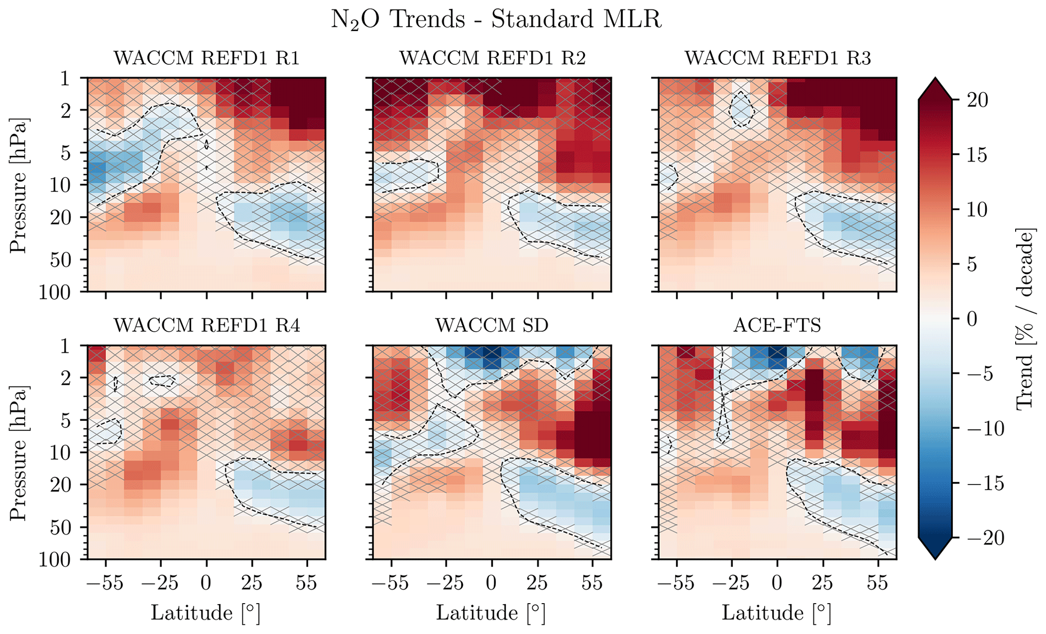
Figure 1N2O trend in ACE-FTS and WACCM for February 2004–December 2018, as calculated with the standard MLR (Eq. 2). R1 to R4 are different ensemble members from the free-running WACCM. Regions with hatching are insignificant at the 2σ level. Dashed contours mark the transitions from positive to negative trends.
The stratospheric N2O trends depend not only on circulation changes, but also on changing N2O surface emissions. This emission trend needs to be removed from the ACE-FTS N2O data and the WACCM N2O results before the N2O can be used as a proxy for dynamics variability. The global surface trend in N2O abundance measured by the NOAA/GML HATS flask programme is calculated using a simple linear regression,
The surface N2O data and the trend lines are shown in the top panel of Fig. 2. The trend is 2.8 % per decade for 2004–2018.
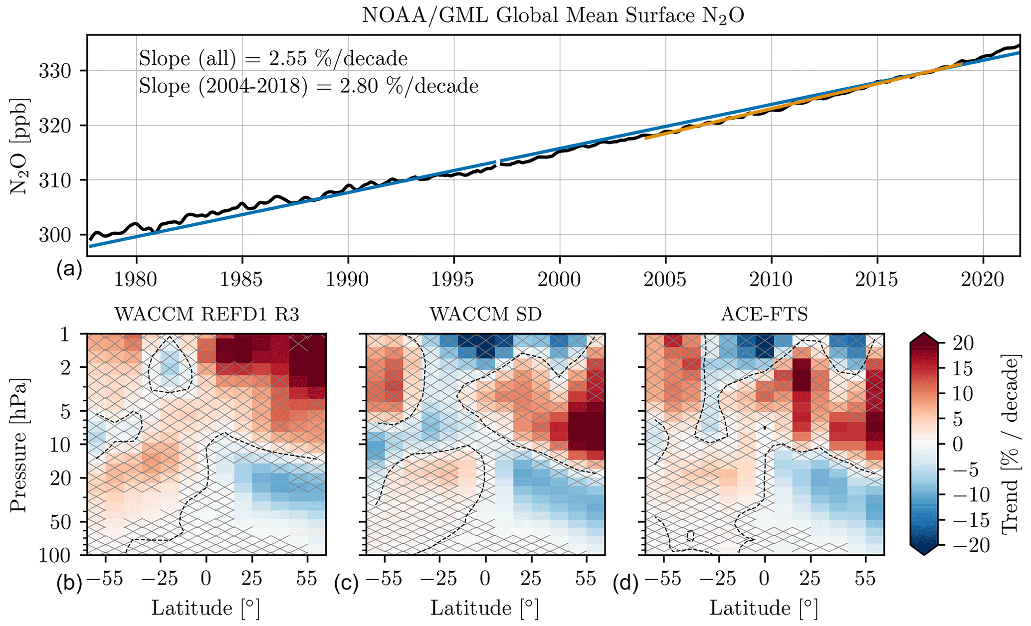
Figure 2(a) Global mean surface N2O trend. The black line is the observations, the blue line is the trend for the full dataset, and the orange line is the trend for 2004–2018. (b) Portion of the stratospheric N2O trend that remains in WACCM and ACE-FTS after the N2O surface trend has been removed. Trends are for February 2004–December 2018 and calculated with the standard MLR (Eq. 2). Regions with hatching are insignificant at the 2σ level. Dashed contours mark the transitions from positive to negative trends.
To construct the N2O regression proxy, the trend in the surface N2O anomaly is subtracted from each latitude and altitude bin of the MZM stratospheric N2O anomalies. By working with the anomaly, we account for differences in the absolute N2O concentrations between the surface N2O measurements and the ACE-FTS measurements or WACCM results. The bottom row of Fig. 2 shows the portion of the N2O trend that remains once the increasing surface N2O emissions are accounted for. Only one free-running WACCM ensemble member is included as an example. We are assuming that this remaining N2O trend is largely due to circulation changes in the atmosphere. There could also be changes in the photolysis rate of N2O and the rate of reaction with O(1D); however, Prather et al. (2023) estimated this effect to be small compared to the total N2O trend: about 1 % per decade in the region of maximum photolysis (30∘ S–30∘ N, 3–15 hPa).
The MZM N2O time series with the surface trend removed is used as a proxy in the N2O MLR equation defined by Stolarski et al. (2018),
The N2O proxy accounts for variability associated with seasonal variations, the QBO, and ENSO, in addition to variability due to a changing BDC. Stolarski et al. (2018) did not consider the effects of the solar cycle and aerosol extinction, even though they have a chemical, rather than dynamical, effect on HCl and ozone. We investigate the effect of including the aerosol and solar cycle proxies in the N2O MLR in Sect. 4.
Trends calculated with the standard MLR and the N2O MLR are compared to assess the ability of N2O to control for stratospheric circulation changes. Two different forms of the N2O MLR are considered, one that uses the ACE-FTS N2O observations as a proxy and one that uses the simulated WACCM N2O as a proxy. The WACCM N2O predictor is either from the corresponding WACCM run (free-running ensemble member or specified dynamics) or from the specified dynamics WACCM run when considering observational data. The specified dynamics run was chosen as it most realistically represents the N2O trend in the ACE-FTS observations (Figs. 1 and 2). While the ACE-FTS measurements are perhaps a better representation of the true stratosphere than WACCM, the sparse ACE-FTS sampling pattern could limit the ability to use ACE-FTS N2O observations as a regression proxy to calculate trends in measurements from other instruments. The ACE-FTS N2O proxy is also limited by the mission lifetime, whereas WACCM can be run for any time period of interest.
We start by examining the HCl trends for latitudes from 60∘ S to 60∘ N and pressure levels from 100 to 1 hPa. This is an update to the results from Stolarski et al. (2018), who focused on a single latitude band, and Bernath et al. (2020), who only discussed the global mean trend. The trend for each latitude–altitude bin is shown in Fig. 3, while the HCl time series and regression fits for four bins are shown in Fig. A2. The top row in Fig. 3 shows the HCl trends calculated with the standard MLR. Only one free-running WACCM ensemble member is included due to the similarity between all four members (the other three are provided in Appendix A, Fig. A3). As with N2O, there is a distinct hemispherical asymmetry in the standard HCl trends below 10 hPa in both the observations and the model runs. This pattern was first observed by Mahieu et al. (2014), who attributed it to a temporary slowdown of the BDC in the NH relative to the SH. The WACCM HCl trend is biased low relative to the ACE-FTS observations: the HCl trend depends on surface emission of chlorine-containing gases, so the lower trend in WACCM suggests that the model is assuming a greater reduction in chlorine emissions than has actually occurred. This could be because the REFD1 model simulations do not include the effect of chlorine-containing very-short-lived source gases (VSL-SGs; Plummer et al., 2021), which have been increasing over the past 20 years (Laube et al., 2022). Hossaini et al. (2019) showed that modelled stratospheric HCl trends are more negative than HCl trends from ACE-FTS when VSL-SGs are not included in the model. Additional model simulations would be required to determine if VSL-SGs are indeed causing the difference between WACCM and ACE-FTS HCl trends.
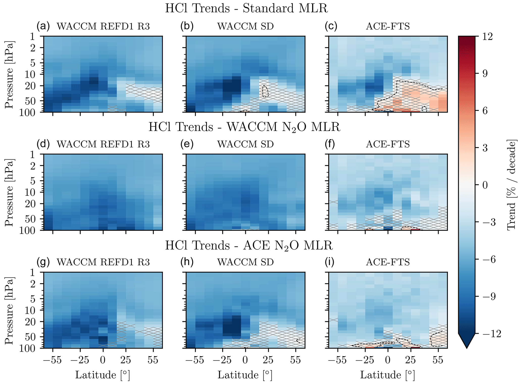
Figure 3HCl trends for February 2004–December 2018. (a, b, c) Trend calculated with standard MLR. (d, e, f) Trends calculated with WACCM N2O MLR. (g, h, i) Trends calculated with ACE-FTS N2O MLR. Regions with hatching are insignificant at the 2σ level. Dashed contours mark the transitions from positive to negative trends.
Figure 3 shows the HCl trends calculated with the WACCM N2O MLR. The largely negative trend is what we expect from decreasing emissions of chlorine-containing source gases. In all cases the N2O regression produces similar trends in the NH and SH, although the trend remains slightly lower in the SH compared to the NH. These results agree with previous studies showing that changes in stratospheric circulation are responsible for the observed increase in NH HCl over the past 2 decades (Mahieu et al., 2014; Stolarski et al., 2018), rather than some unaccounted for source of HCl in the NH.
Using ACE-FTS N2O as the regression proxy works well for ACE-FTS observations but not for WACCM simulations (bottom row of Fig. 3). In the case of the ACE-FTS observations, the HCl trend in the NH is greatly reduced when either WACCM N2O or ACE-FTS N2O is used as the regression proxy (the HCl trend in the SH increases slightly more when the ACE-FTS N2O is used in the MLR instead of the WACCM N2O). However, when ACE-FTS N2O is used as a regression proxy to calculate WACCM HCl trends, there is a clear hemispheric asymmetry remaining. This can also be seen by looking at the goodness of fit (R2) for the different versions of the MLR (Fig. A4). The fit to HCl is generally better when using the N2O MLR instead of the standard MLR, but only when the N2O is from the same dataset (i.e. when WACCM N2O is fit to WACCM HCl or ACE-FTS N2O is fit to ACE-FTS HCl). This suggests that ACE-FTS N2O observations only work well as a stratospheric circulation proxy for calculating trends in gases measured by ACE-FTS, when there is a perfect sampling match. We also note the inclusion of aerosol and/or solar cycle proxies in the N2O MLR has a negligible impact on the HCl trends – this is shown for the ACE-FTS observations in Appendix A, Fig. A5.
The comparison with the standard HCl trends demonstrates that the N2O MLR removes most of the positive or insignificant HCl trends by accounting for signals of dynamical variability. Based on this result, we next used the N2O proxy to determine O3 trends accounting for changes in stratospheric circulation. The top row of Fig. 4 shows the O3 trends for February 2004–December 2018 from the standard MLR (the remaining free-running WACCM ensemble members are shown in Appendix A, Fig. A7, and the time series for several bins is shown in Fig. A6). The standard trends are broadly consistent between all WACCM runs and the ACE-FTS observations: O3 is increasing above 10 hPa and in the SH, although this increase is less significant in ACE-FTS O3 than in WACCM O3. In all cases there is a tongue of decreasing trend from about 40 to 10 hPa in the NH, with a smaller region of negative trend extending down to 100 hPa. These negative trends in the tropics and NH are a known feature of O3 trends in the 21st century that have been broadly attributed to circulation changes (e.g. Ball et al., 2019, 2020; Bognar et al., 2022; Godin-Beekmann et al., 2022).
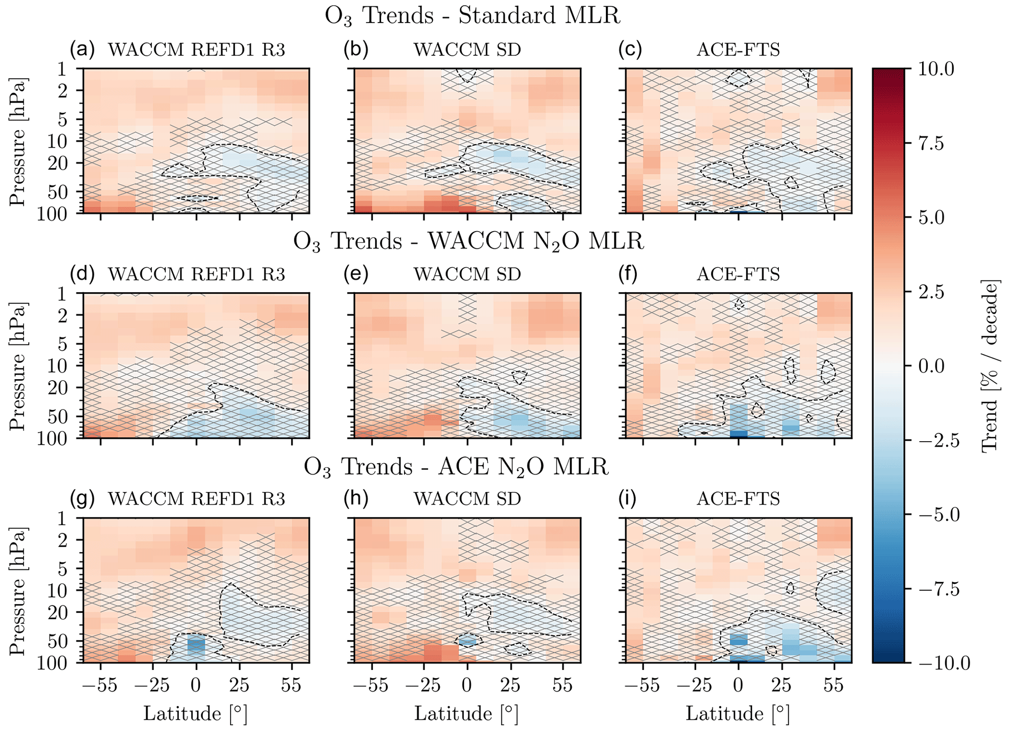
Figure 4O3 trends for February 2004–December 2018. (a, b, c) Trend calculated with standard MLR. (d, e, f) Trends calculated with WACCM N2O MLR. (g, h, i) Trends calculated with ACE-FTS N2O MLR. Regions with hatching are insignificant at the 2σ level. Dashed contours mark the transitions from positive to negative trends.
The WACCM N2O MLR successfully accounts for the negative ozone trend in the NH above ∼ 30 hPa: the bins of significant negative trend become insignificant and positive (middle row of Fig. 4). At the same time, the WACCM N2O MLR enhances the region of (largely insignificant) negative ozone trend in the NH and tropics below 30 hPa. The O3 trends for ACE-FTS are similar whether WACCM or ACE-FTS N2O is used as the regression proxy; however, using ACE-FTS N2O as a proxy for calculating trends in WACCM O3 results in trends that are more similar to those from the standard MLR than from the WACCM N2O MLR. The goodness of fit coefficients for each version of the MLR are shown in Appendix A, Fig. A8. As with HCl, the fit is best when N2O from the same dataset is used. In certain regions the R2 value is higher for the standard MLR than for the N2O MLR: this corresponds to areas where there is a weak relationship between N2O and O3 (see Fig. 5 and the following paragraphs). As with HCl, the inclusion of a proxy for the solar cycle or for aerosols has a minimal effect on the O3 trends from the N2O regression (Appendix A, Fig. A5). Therefore changes in aerosol levels or solar radiation levels are not significantly impacting stratospheric O3 trends over 2004–2018.
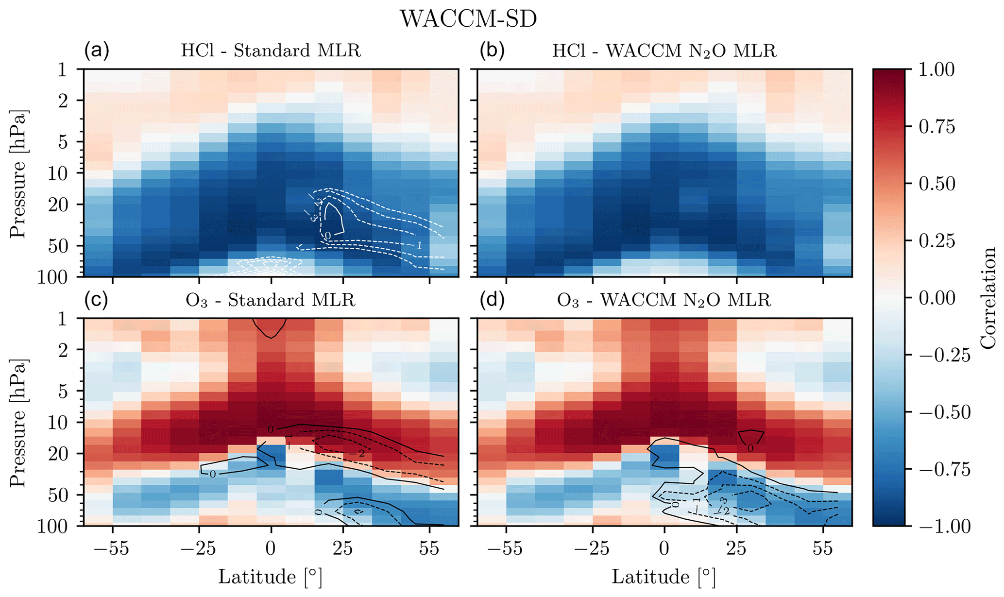
Figure 5(a, b) Correlation coefficient for WACCM-SD HCl and N2O. White contours show where the HCl trend is greater than −3 % per decade. (c, d) Correlation coefficient for WACCM-SD O3 and N2O. Black contours show where the O3 trend is less than 0 % per decade. The trend contours in the left row were calculated with the standard MLR, and the trend contours in the right row were calculated with the N2O MLR.
The effect that the N2O proxy has on both O3 and HCl trends can be understood by considering the relationships between the gases. The level of correlation between HCl and N2O is shown in the top row of Fig. 5 for the WACCM-SD run. N2O and HCl are anti-correlated throughout the lower and mid-stratosphere because N2O is a long-lived trace gas with a tropospheric source and because HCl is a long-lived trace gas with a stratospheric source. While the anti-correlation is largely due to transport-driven variability on shorter timescales, it also implies that long-term changes in transport will have opposite effects on N2O and HCl. The anti-correlation between HCl and N2O is thus consistent with their trends from the standard MLR being of opposite sign everywhere below 10 hPa and indicates that the latter are driven by long-term changes in transport. The contour lines in the top left panel of Fig. 5 show where the HCl trend is greater than −3 % per decade, clearly outlining the region where the standard MLR computes a trend that is inconsistent with tropospheric chlorine trends. In this same region, the dynamical component of the N2O trend is negative (Fig. 2). Fitting the N2O proxy to remove the portion of the HCl trend caused by transport lowers the resulting HCl trend in the NH, which is now consistent with the chemical signal from the tropospheric chlorine trends. At the same time, it increases the HCl trend in the SH, successfully removing the difference in HCl trends between the hemispheres.
Turning now to O3, the bottom row of Fig. 5 shows that O3 is anti-correlated with N2O below ∼ 30 hPa and correlated above. Above ∼ 30 hPa, the lifetime of O3 is largely defined by chemical production and loss, while below ∼ 30 hPa the O3 distribution is controlled by transport. As with N2O and HCl, the transport-driven anti-correlation between N2O and O3 below ∼ 30 hPa suggests that long-term changes in stratospheric circulation will have an opposite effect on N2O and O3 in this region. Therefore fitting the N2O proxy to account for the portion of the O3 trend caused by transport lowers the O3 trend in the NH, where the dynamical N2O trend is negative. Conversely, between ∼ 10 and 30 hPa in the NH, O3 and N2O are correlated and the dynamical N2O trend is negative, so fitting the N2O proxy to O3 increases the O3 trend (compared to the standard MLR trend). The black contour lines in the bottom row of Fig. 5 show where the O3 trend is zero or negative for each version of the MLR, illustrating the increase in the O3 trend in the NH above 30 hPa and the decrease in the O3 trend in the NH below 30 hPa. Overall, using the N2O MLR instead of the standard MLR reduces the hemispheric asymmetry in O3 trends above 30 hPa but increases the asymmetry below 30 hPa. Below 30 hPa, changes to the stratospheric circulation induce a positive ozone trend, so there must be some other reason for the negative or insignificant trend that is observed in this region when using the standard MLR.
We now investigate using the N2O MLR to calculate trends in OSIRIS O3. Figure 6 shows the OSIRIS O3 trends from the standard MLR, the N2O MLR with WACCM-SD N2O, and the N2O MLR with ACE-FTS N2O. The trends are overall very similar to those for WACCM and ACE-FTS O3, with the negative trend from 10–30 hPa in the NH disappearing when the N2O MLR is used instead of the standard MLR. N2O from both ACE-FTS and WACCM-SD work equally well as dynamical proxies for calculating OSIRIS O3 trends. This provides confidence that the N2O observations from ACE-FTS or simulations from WACCM can be used to determine trends in an independent observational dataset.
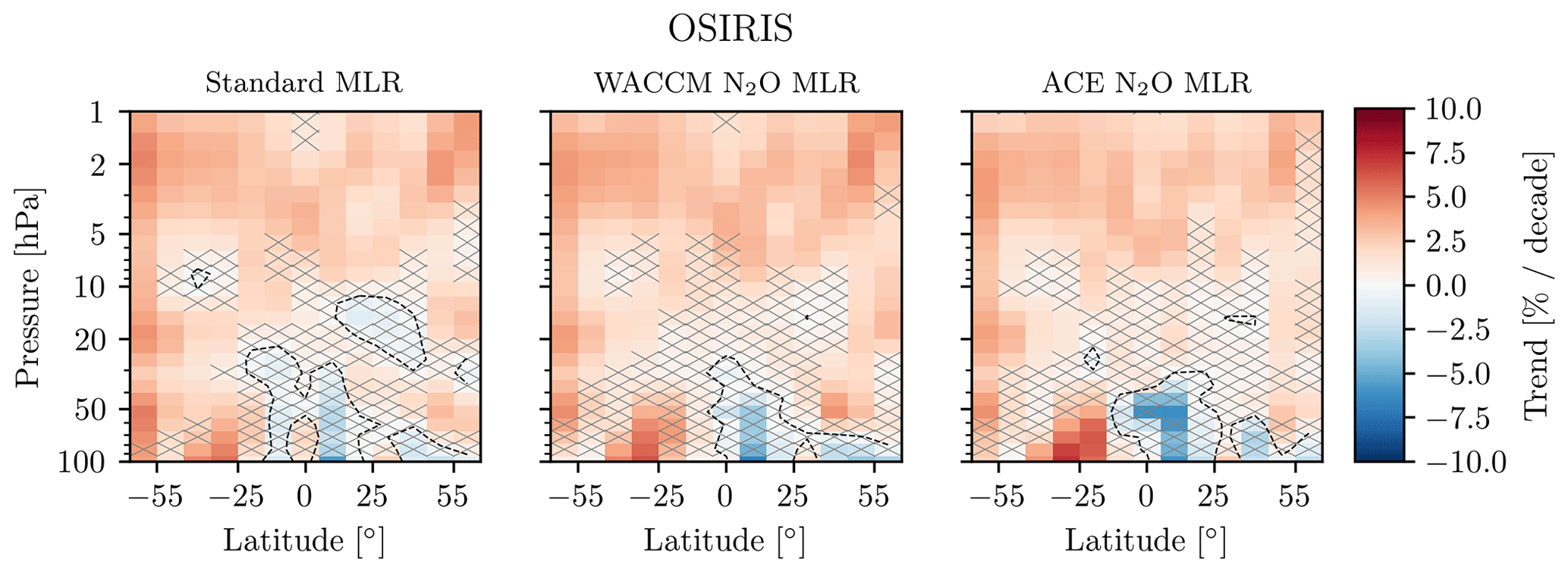
Figure 6OSIRIS O3 trends for February 2004–December 2018. Regions with hatching are insignificant at the 2σ level. Dashed contours mark the transitions from positive to negative trends.
The N2O regression can also be used to study NOy trends. Surface N2O emissions are the main source of stratospheric NOy, and both NOy and N2O are impacted by BDC changes. By controlling for these effects, the N2O regression can be used to determine if the NOy trend is consistent with increasing N2O surface emissions or if there is some other factor affecting the NOy trend. The NOy trend from the standard MLR is shown in the top row of Fig. 7, and the time series for four bins are shown in Fig. A9. The ACE-FTS sunrise and sunset occultations are kept separate to avoid any diurnal effects in the NOy species. As with N2O and HCl, there is a distinct hemispheric asymmetry in the NOy trends from the standard regression. The positive trends in the NH below 10 hPa have similar magnitudes for both WACCM and ACE-FTS, but the negative trend in the SH is lower in ACE-FTS observations compared to the WACCM results. The WACCM trends look the same if the WACCM NOy is limited to the five gases used to calculate the ACE-FTS NOy, so this is not the reason for the difference between their trends. It is possible that the differences between WACCM and ACE-FTS NOy are due to differences in local time as the ACE-FTS NOy trends agree better with WACCM at sunset than sunrise, particularly in the NH. The WACCM NOy results are a daily mean rather than calculated at a specific local time.
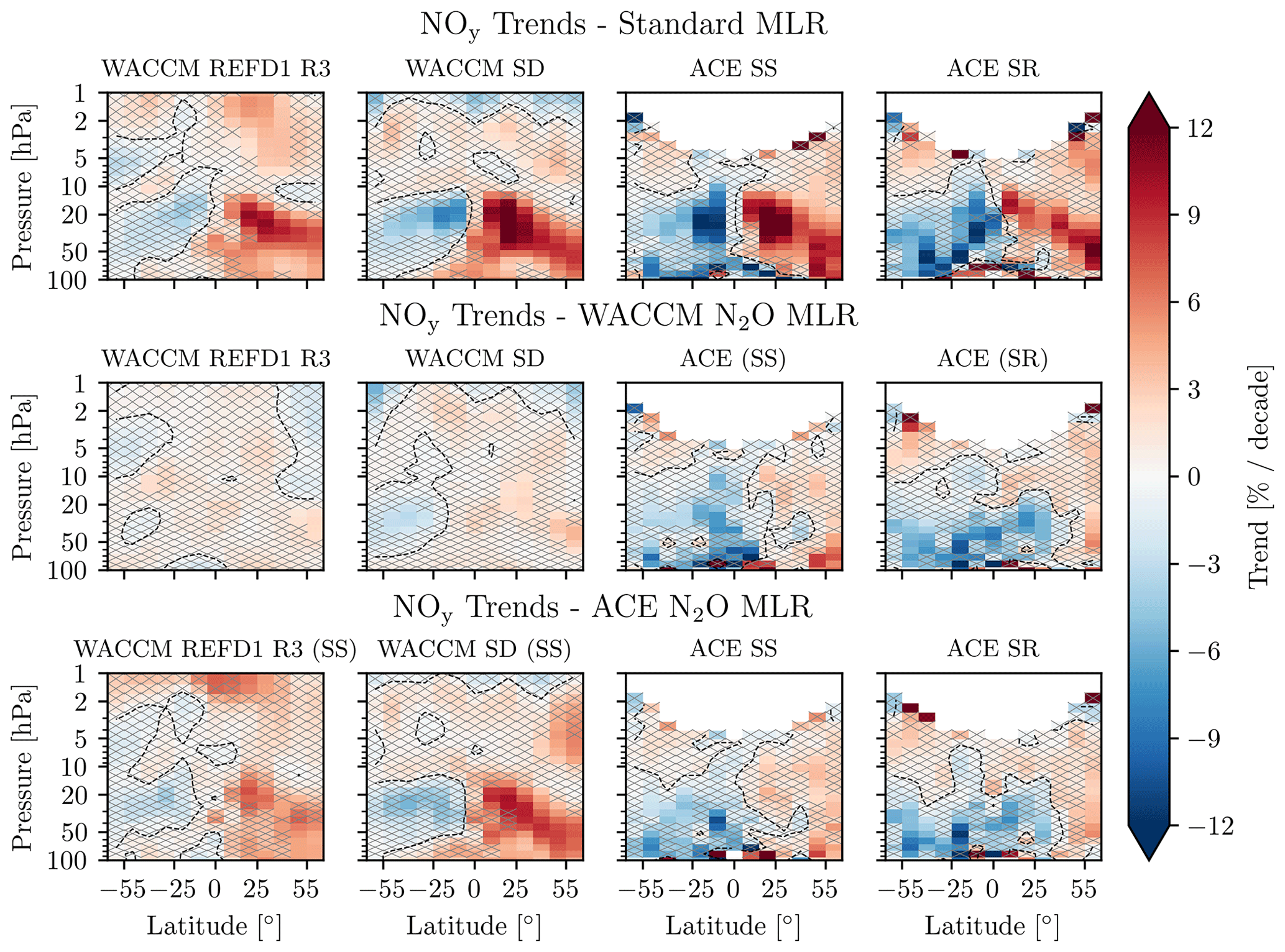
Figure 7NOy trends for February 2004–December 2018. Top row: trend calculated with standard MLR. Centre row: trends calculated with WACCM N2O MLR. Bottom row: trends calculated with ACE-FTS N2O MLR. Regions with hatching are insignificant at the 2σ level. Dashed contours mark the transitions from positive to negative trends.
N2O is the main source of NOy, so we expect that using the N2O regression to account for the effect of dynamics will result in an NOy trend with a comparable magnitude to the N2O emissions trend (2.8 % per decade). This does occur in the case of WACCM – both the REFD1 simulations and the specified dynamics run have insignificant trends on the order of 1 % per decade to 3 % per decade, as calculated with the WACCM N2O regression (middle row of Fig. 7). However, using the N2O regression (with either WACCM or ACE-FTS N2O) on ACE-FTS NOy observations results in a largely negative and significant trend. As with HCl and O3, using ACE-FTS N2O observations as a regression proxy for WACCM NOy does not adequately account for the trend difference between the hemispheres.
Since N2O is the main source of NOy, these gases are anti-correlated throughout much of the stratosphere. This means that when using the N2O proxy, the positive N2O trend in the SH will increase the NOy trend in the SH, making it less negative. Similarly, in the NH, the negative trend in the N2O proxy will make the NOy trend less positive. For WACCM, the magnitudes of the N2O and NOy trends from the standard regression are similar, so we see the expected cancellation in the N2O regression. For ACE-FTS, the NOy trends in the SH are lower than expected based on the N2O trend, so the N2O proxy cannot fully explain the decreasing NOy. However, the overall changes in the trends when using the N2O MLR instead of the standard MLR are consistent with what we expect from the relationship between NOy and N2O. Further understanding the differences between ACE-FTS and WACCM NOy trends requires a more detailed study.
Several recent studies showed that stratospheric ozone has declined in the tropics and NH throughout the 21st century, despite the overall success of the Montreal Protocol in reducing ozone depletion in the SH and upper stratosphere (e.g. Ball et al., 2018, 2019; SPARC/IO3C/GAW, 2019; Bognar et al., 2022; Godin-Beekmann et al., 2022). The remaining negative ozone trend is thought to be caused by changes in the BDC that result in air moving slower and deeper through the stratosphere in the NH relative to the SH (e.g. Ploeger and Garny, 2022; Strahan et al., 2020). The present work uses N2O observations from ACE-FTS and simulations from WACCM to account for BDC changes in the MLR used to calculate ozone trends.
Ozone trends from 2004–2018 are consistent between observations from OSIRIS and ACE-FTS. Trends in O3 simulations from both free-running and specified dynamics WACCM runs also agree very well with the observational trends. N2O time series from both WACCM and ACE-FTS work well as a regression proxy for O3 from OSIRIS, but the ACE-FTS N2O MLR does not improve upon the results of the standard MLR when calculating WACCM O3 trends. For each dataset, the standard MLR results show an O3 decrease in the NH between about 10 and 30 hPa, as well as O3 decrease at lower levels. The results of using the N2O MLR to determine stratospheric O3 trends imply that long-term circulation changes are causing O3 to increase in the NH relative to the SH. By using the N2O MLR instead of the standard MLR, the negative O3 trend in the NH above 30 hPa is eliminated or becomes insignificant. However, the N2O proxy cannot explain the negative O3 trends that are observed in results from the standard MLR in the NH below 30 hPa. In fact, our results suggest that long-term circulation changes are causing an increase in O3 in the NH below 30 hPa. This transport-induced O3 increase is consistent with the HCl increase in the same region: a long-term transport slowdown causes gases with a stratospheric source and a long chemical lifetime to have an increasing trend.
These O3 trend results agree with those from Weber et al. (2022), who found that including proxies for dynamical variability in the standard MLR model increased column O3 trends in the NH but did not change column O3 trends in the tropics. It is possible that the negative O3 trend below 30 hPa is due to changes in the tropopause height rather than in upwelling. Bognar et al. (2022) found that using tropopause relative coordinates reduced the significance and magnitude of the negative O3 trends over 2000–2021 in the tropics, up to 7 km above the tropopause. The N2O proxy cannot account for changes in the tropopause height because N2O is relatively inert in both the upper troposphere and lower stratosphere (i.e. Fig. 2; the N2O trend in the tropical stratosphere below 50 hPa is the same as the surface N2O trend). It should also be noted that our results differ from those of Orbe et al. (2020) and Wargan et al. (2018), who attributed the negative O3 trend in the NH below 30 hPa to circulation changes. The difference could be due to the different time period analyzed (1998–2016 instead of 2004–2018). These studies also relied on an idealized e90 tracer rather than observations of N2O
N2O from WACCM successfully accounts for the hemispherical asymmetry that is present in HCl trends computed using the standard MLR. N2O from ACE-FTS can also be used as a regression proxy, but it works best when considering other ACE-FTS observations rather than WACCM results. The ability of the N2O proxies to explain the HCl increase in the NH implies that this increase is not caused by rising chlorine emissions but rather by changes in transport. This is consistent with observations showing that chlorine emissions have largely been declining (Laube et al., 2022).
Lastly, we showed that trends in NOy determined using the standard MLR have a strong asymmetry, with negative trends in the SH and positive trends in the NH. This is true for both ACE-FTS observations and in WACCM simulations. When using the N2O MLR to find the NOy trends, the WACCM NOy trends become mostly insignificant and have a similar magnitude as the N2O surface emissions. This is what is expected, as the main NOy source is N2O. This is not the case for the ACE-FTS NOy trends, which are significantly negative in most bins when calculated with the N2O MLR. Despite this, the ACE-FTS NOy trends from the N2O MLR are consistent with what is expected from the relationship between N2O and NOy, given the trends from the standard MLR.
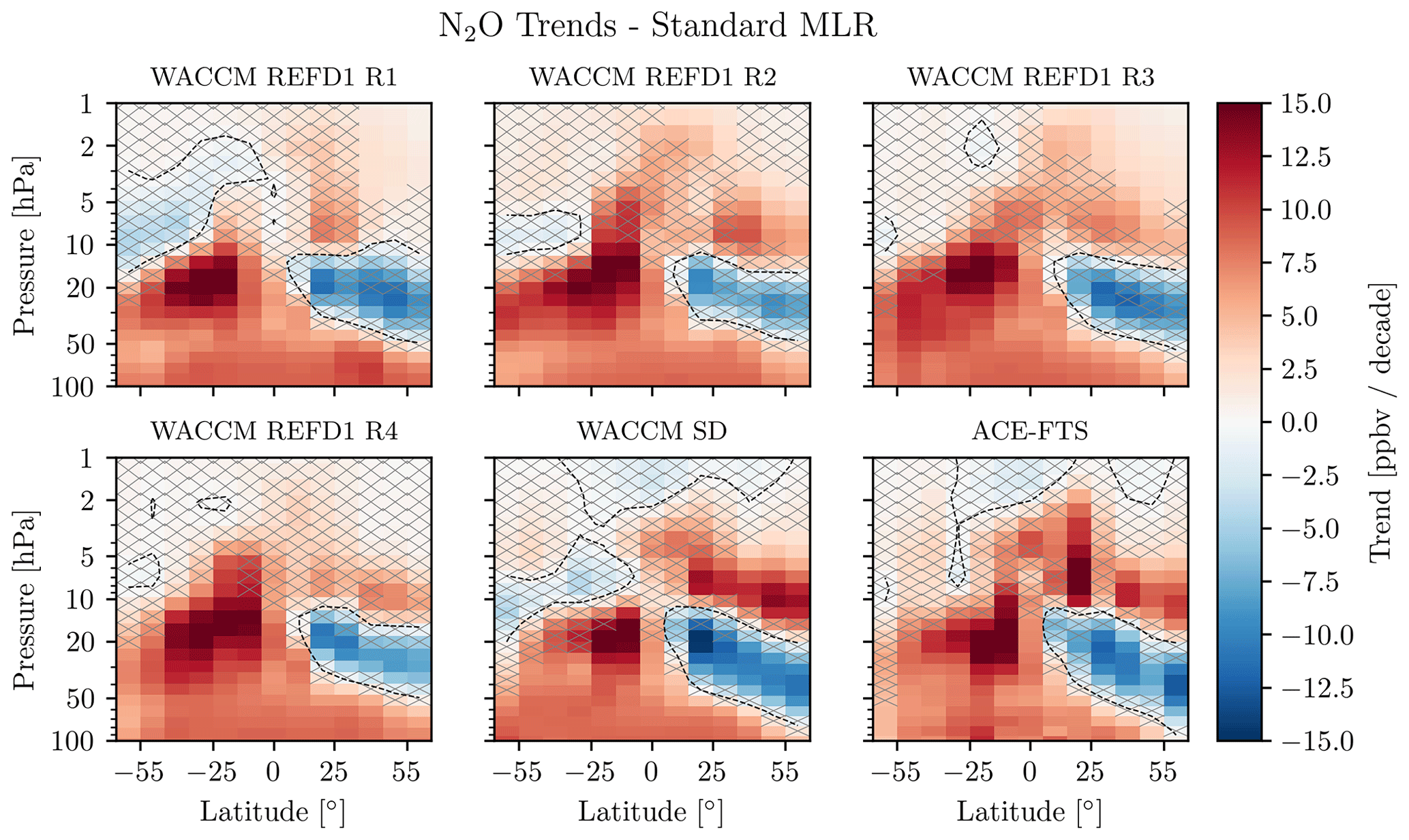
Figure A1N2O trend in ACE-FTS and WACCM trends in units of ppbv per decade for February 2004–December 2018, as calculated with the standard MLR (Eq. 2). Regions with hatching are insignificant at the 2σ level. Dashed contours mark the transitions from positive to negative trends.
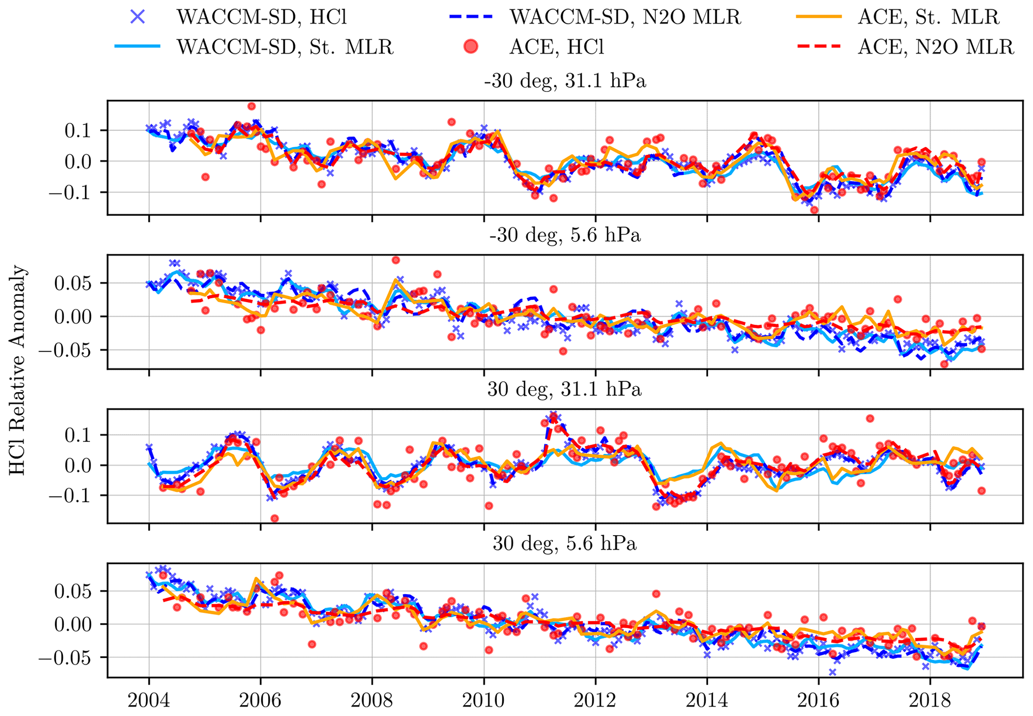
Figure A2Relative anomaly and MLR fits for WACCM-SD and ACE-FTS HCl in four latitude–pressure bins. The “St.” label refers to the standard MLR.
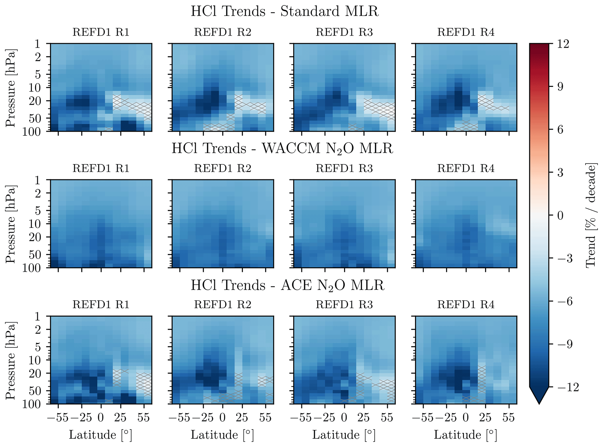
Figure A3WACCM REFD1 HCl trends for February 2004–December 2018. Top row: trend calculated with standard MLR. Centre row: trends calculated with WACCM N2O MLR. Bottom row: trends calculated with ACE-FTS N2O MLR. Regions with hatching are insignificant at the 2σ level.
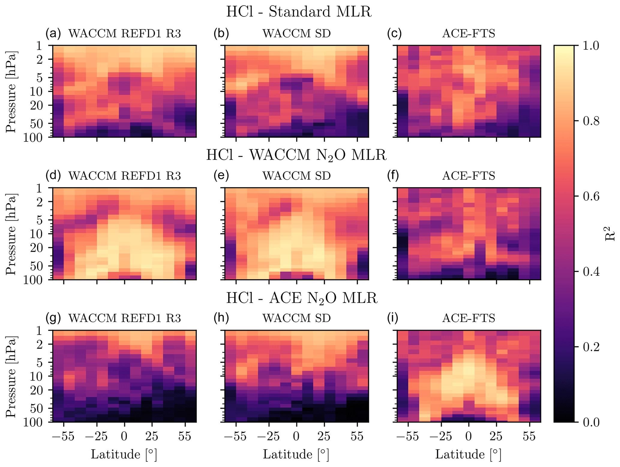
Figure A4Goodness of fit for ACE-FTS and WACCM HCl. (a, b, c) R2 for standard MLR. (d, e, f) R2 for WACCM N2O MLR. (g, h, i) R2 for ACE-FTS N2O MLR.
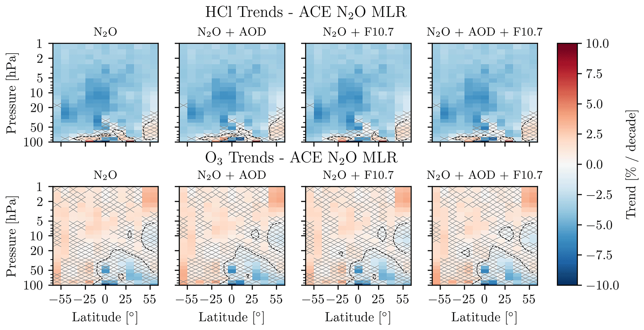
Figure A5ACE-FTS trends for February 2004–December 2018. Top row: HCl trends calculated with ACE N2O MLR. Bottom row: O3 trends calculated with ACE-FTS N2O MLR. Regions with hatching are insignificant at the 2σ level.
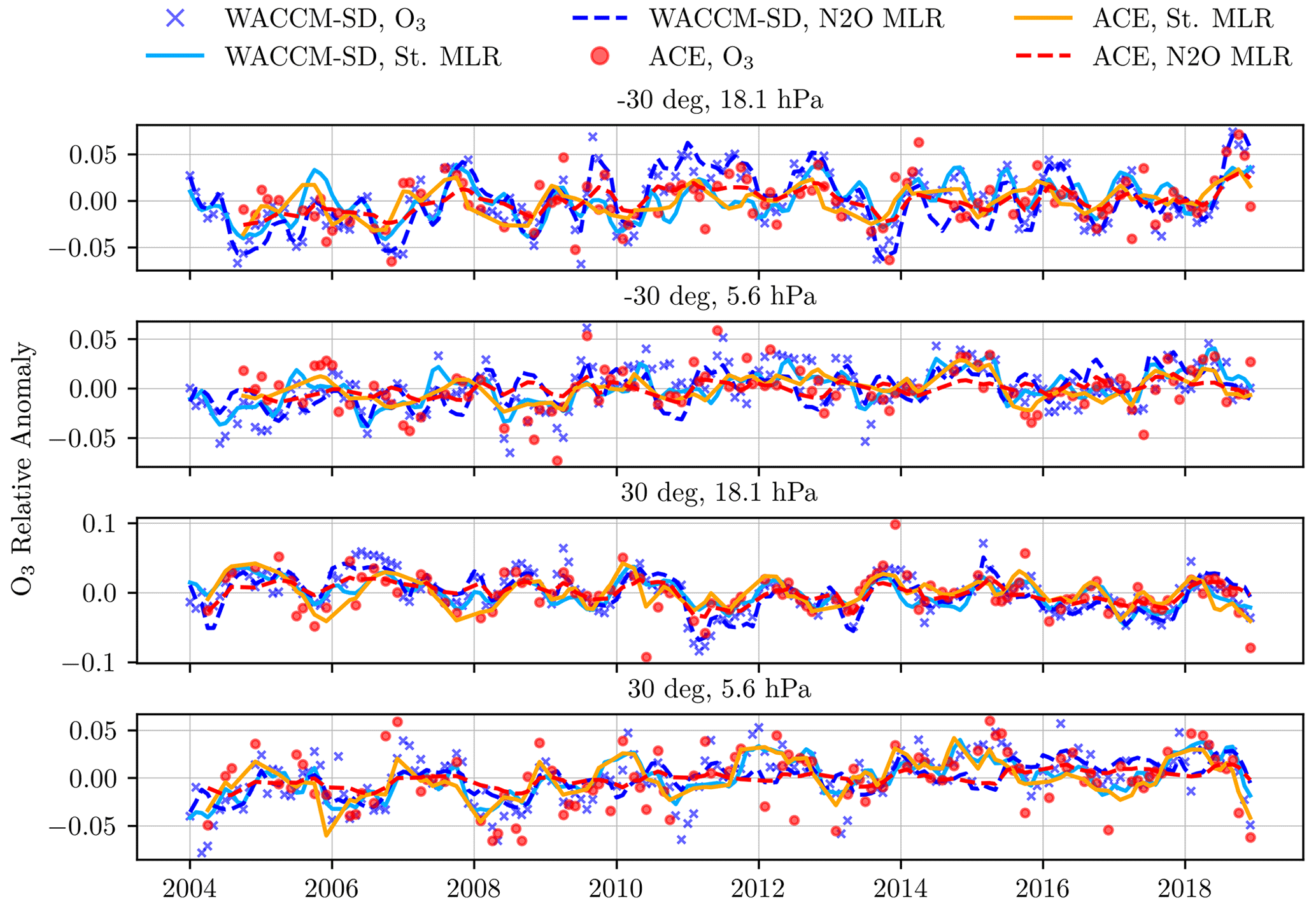
Figure A6Relative anomaly and MLR fits for WACCM-SD and ACE-FTS O3 in four latitude–pressure bins. The “St.” label refers to the standard MLR.
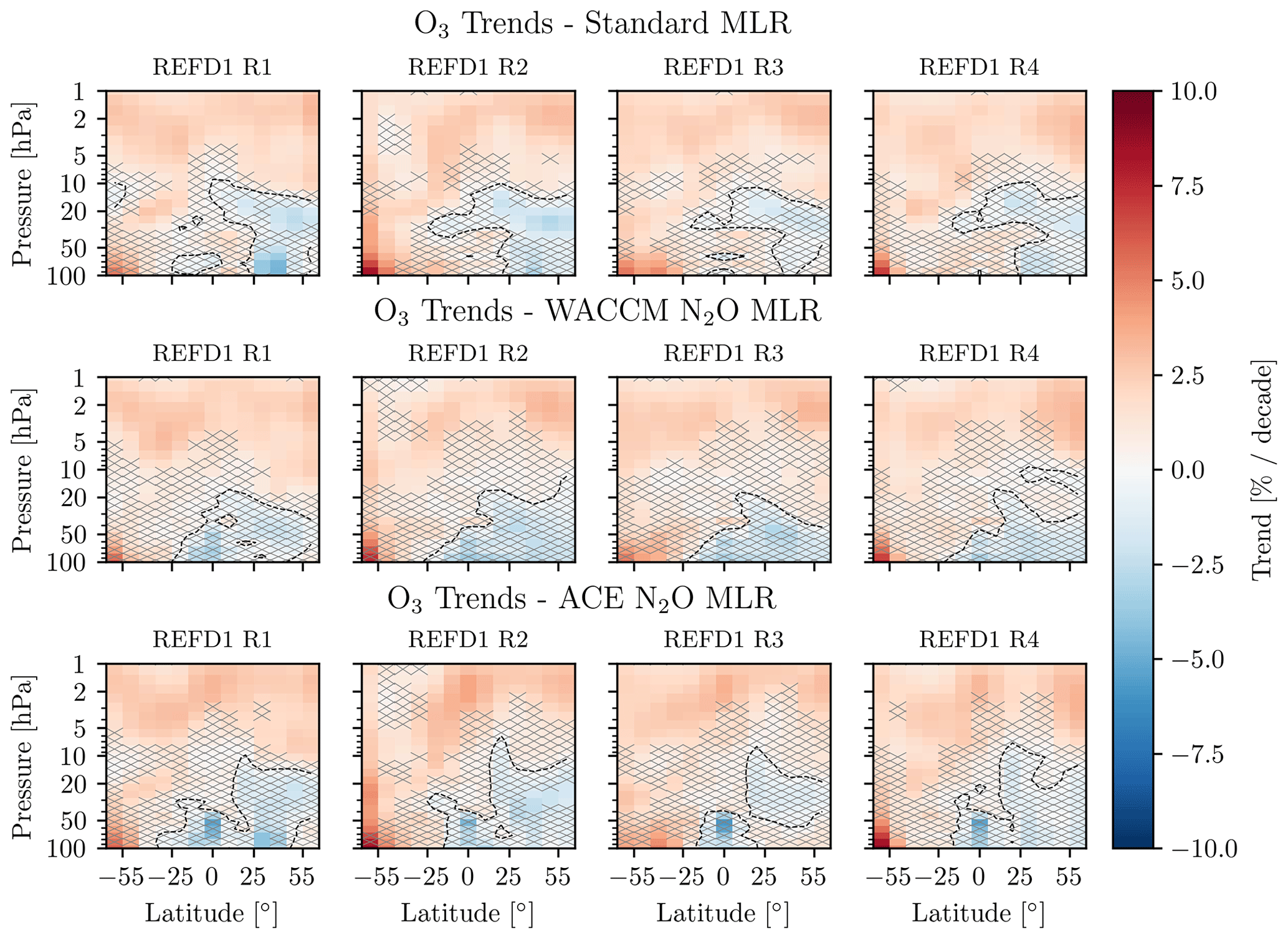
Figure A7WACCM REFD1 O3 trends for February 2004–December 2018. Top row: trend calculated with standard MLR. Centre row: trends calculated with WACCM N2O MLR. Bottom row: trends calculated with ACE-FTS N2O MLR. Regions with hatching are insignificant at the 2σ level.
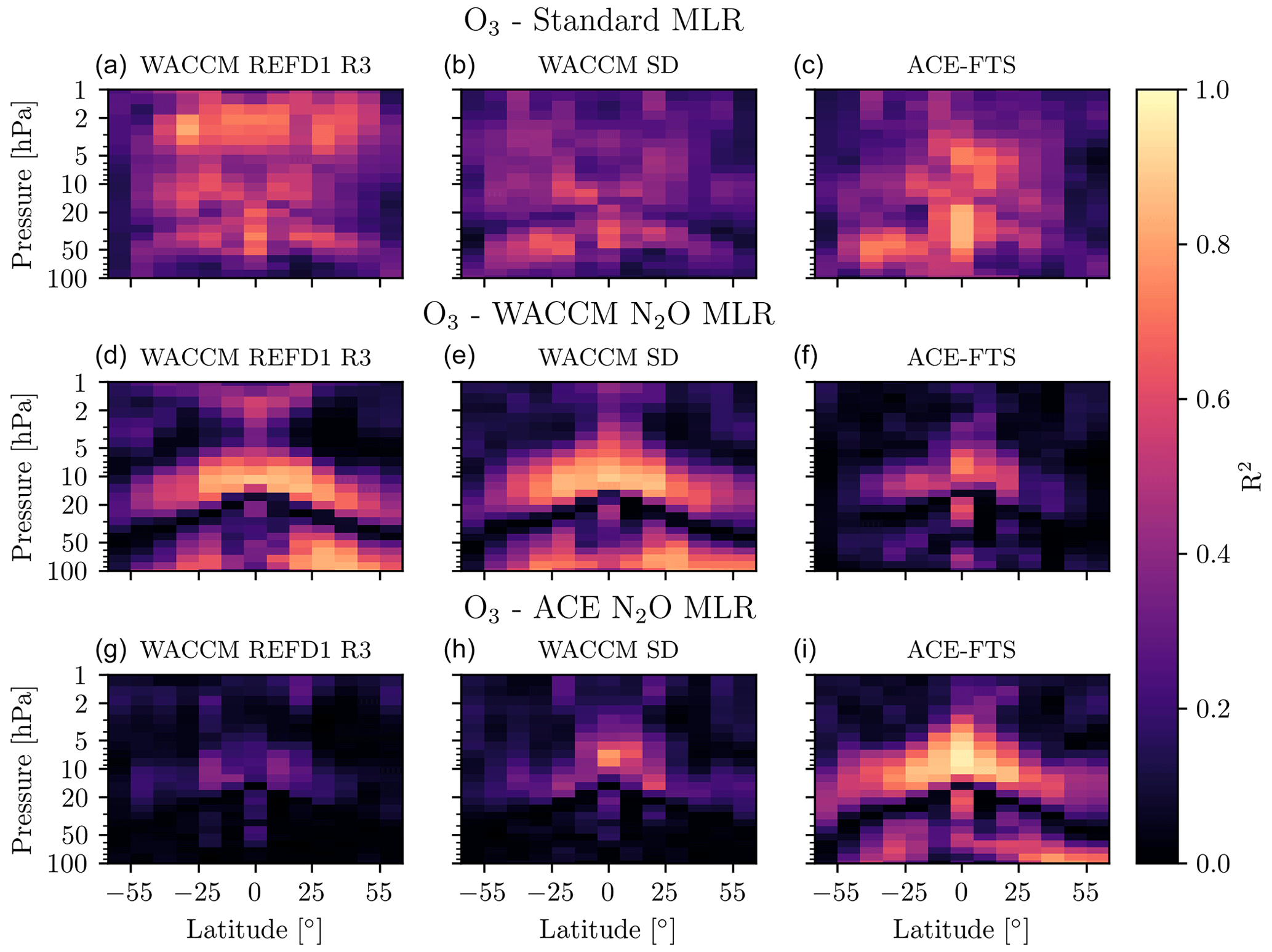
Figure A8Goodness of fit for ACE-FTS and WACCM O3. (a, b, c) R2 for standard MLR. (d, e, f) R2 for WACCM N2O MLR. (g, h, i) R2 for ACE-FTS N2O MLR.
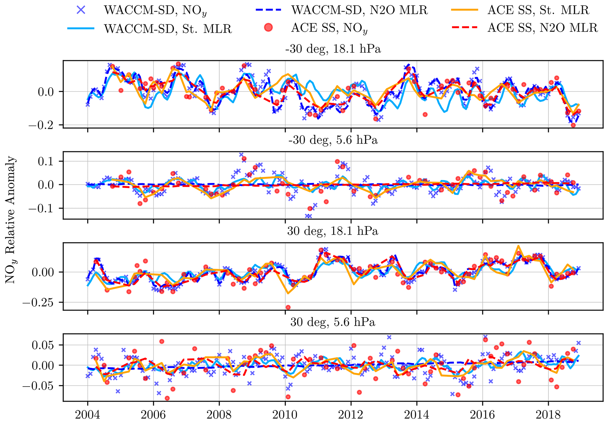
Figure A9Relative anomaly and MLR fits for WACCM-SD and ACE-FTS NOy in four latitude–pressure bins. The “St.” label refers to the standard MLR. Only ACE-FTS sunset (SS) occultations are shown to minimize the number of lines on the plot.
OSIRIS data are available at https://research-groups.usask.ca/osiris/data-products.php#OSIRISLevel2DataProducts (Zawada et al., 2022).
The WACCM results are available at ftp://odin-osiris.usask.ca/Models (OSIRIS team, 2022b).
Instructions for downloading the OSIRIS and WACCM files are at https://research-groups.usask.ca/osiris/data-products.php#Download (OSIRIS team, 2022a).
ACE-FTS data are available at https://databace.scisat.ca/level2/ (ACE-FTS, 2022).
ACE-FTS data quality flags are available at https://doi.org/10.5683/SP2/BC4ATC (Sheese and Walker, 2022).
The NOAA/GML HATS N2O data are available at https://gml.noaa.gov/hats/combined/N2O.html (NOAA/GML, 2022).
The LOTUS regression code and documentation are available at https://arg.usask.ca/docs/LOTUS_regression/index.html (Damadeo et al., 2022).
KD performed the analysis and prepared the manuscript. ST, AB, DZ, and DD provided input on the method and analysis. PES and KAW provided guidance on using the ACE-FTS data. WR provided the WACCM results. All authors provided significant feedback on the manuscript.
The contact author has declared that none of the authors has any competing interests.
Publisher’s note: Copernicus Publications remains neutral with regard to jurisdictional claims made in the text, published maps, institutional affiliations, or any other geographical representation in this paper. While Copernicus Publications makes every effort to include appropriate place names, the final responsibility lies with the authors.
The authors thank the Swedish National Space Agency and the Canadian Space Agency for the continued operation and support of Odin-OSIRIS. The Atmospheric Chemistry Experiment (ACE) is a Canadian-led mission mainly supported by the CSA and the NSERC, and Peter Bernath is the principal investigator. The National Center for Atmospheric Research is sponsored by the US National Science Foundation. This research was enabled by the computational and storage resources of NCAR's Computational and Information Systems Laboratory (CISL), sponsored by the NSF. Cheyenne: HPE/SGI ICE XA System (NCAR Community Computing). Boulder, CO: National Center for Atmospheric Research. https://doi.org/10.5065/D6RX99HX (last access: 24 May 2023).
This research has been supported by the Canadian Space Agency (grant no. 21SUASULSO). William Randel was also supported as part of the Aura Science Team under NASA grant no. 80NSSC20K0928.
This paper was edited by Gabriele Stiller and reviewed by Sandip Dhomse and one anonymous referee.
Abalos, M., Polvani, L., Calvo, N., Kinnison, D., Ploeger, F., Randel, W., and Solomon, S.: New Insights on the Impact of Ozone-Depleting Substances on the Brewer-Dobson Circulation, J. Geophys. Res.-Atmos., 124, 2435–2451, https://doi.org/10.1029/2018JD029301, 2019. a
Abalos, M., Calvo, N., Benito-Barca, S., Garny, H., Hardiman, S. C., Lin, P., Andrews, M. B., Butchart, N., Garcia, R., Orbe, C., Saint-Martin, D., Watanabe, S., and Yoshida, K.: The Brewer–Dobson circulation in CMIP6, Atmos. Chem. Phys., 21, 13571–13591, https://doi.org/10.5194/acp-21-13571-2021, 2021. a
ACE-FTS: Level 2 Data, Version 4.1/4.2, Federated Research Data Repository [data set], https://databace.scisat.ca/level2/ (last access: 5 October 2022), 2022. a
Ball, W. T., Alsing, J., Mortlock, D. J., Staehelin, J., Haigh, J. D., Peter, T., Tummon, F., Stübi, R., Stenke, A., Anderson, J., Bourassa, A., Davis, S. M., Degenstein, D., Frith, S., Froidevaux, L., Roth, C., Sofieva, V., Wang, R., Wild, J., Yu, P., Ziemke, J. R., and Rozanov, E. V.: Evidence for a continuous decline in lower stratospheric ozone offsetting ozone layer recovery, Atmos. Chem. Phys., 18, 1379–1394, https://doi.org/10.5194/acp-18-1379-2018, 2018. a, b, c
Ball, W. T., Alsing, J., Staehelin, J., Davis, S. M., Froidevaux, L., and Peter, T.: Stratospheric ozone trends for 1985–2018: sensitivity to recent large variability, Atmos. Chem. Phys., 19, 12731–12748, https://doi.org/10.5194/acp-19-12731-2019, 2019. a, b, c, d
Ball, W. T., Chiodo, G., Abalos, M., Alsing, J., and Stenke, A.: Inconsistencies between chemistry–climate models and observed lower stratospheric ozone trends since 1998, Atmos. Chem. Phys., 20, 9737–9752, https://doi.org/10.5194/acp-20-9737-2020, 2020. a
Bernath, P. and Fernando, A. M.: Trends in stratospheric HCl from the ACE satellite mission, J. Quant. Spectrosc. Ra., 217, 126–129, https://doi.org/10.1016/j.jqsrt.2018.05.027, 2018. a, b
Bernath, P., Steffen, J., Crouse, J., and Boone, C.: Sixteen-year trends in atmospheric trace gases from orbit, J. Quant. Spectrosc. Ra., 253, 107178, https://doi.org/10.1016/j.jqsrt.2020.107178, 2020. a
Bernath, P. F., McElroy, C. T., Abrams, M. C., Boone, C. D., Butler, M., Camy-Peyret, C., Carleer, M., Clerbaux, C., Coheur, P.-F., Colin, R., DeCola, P., DeMazière, M., Drummond, J. R., Dufour, D., Evans, W. F. J., Fast, H., Fussen, D., Gilbert, K., Jennings, D. E., Llewellyn, E. J., Lowe, R. P., Mahieu, E., McConnell, J. C., McHugh, M., McLeod, S. D., Michaud, R., Midwinter, C., Nassar, R., Nichitiu, F., Nowlan, C., Rinsland, C. P., Rochon, Y. J., Rowlands, N., Semeniuk, K., Simon, P., Skelton, R., Sloan, J. J., Soucy, M.-A., Strong, K., Tremblay, P., Turnbull, D., Walker, K. A., Walkty, I., Wardle, D. A., Wehrle, V., Zander, R., and Zou, J.: Atmospheric Chemistry Experiment (ACE): Mission overview, Geophys. Res. Lett., 32, L15S01, https://doi.org/10.1029/2005GL022386, 2005. a, b
Bognar, K., Tegtmeier, S., Bourassa, A., Roth, C., Warnock, T., Zawada, D., and Degenstein, D.: Stratospheric ozone trends for 1984–2021 in the SAGE II–OSIRIS–SAGE III/ISS composite dataset, Atmos. Chem. Phys., 22, 9553–9569, https://doi.org/10.5194/acp-22-9553-2022, 2022. a, b, c, d, e, f, g
Boone, C., Bernath, P., Cok, D., Jones, S., and Steffen, J.: Version 4 retrievals for the atmospheric chemistry experiment Fourier transform spectrometer (ACE-FTS) and imagers, J. Quant. Spectrosc. Ra., 247, 106939, https://doi.org/10.1016/j.jqsrt.2020.106939, 2020. a
Boone, C. D., Nassar, R., Walker, K. A., Rochon, Y., McLeod, S. D., Rinsland, C. P., and Bernath, P. F.: Retrievals for the atmospheric chemistry experiment Fourier-transform spectrometer, Appl. Optics, 44, 7218–7231, https://doi.org/10.1364/AO.44.007218, 2005. a
Bourassa, A. E., Roth, C. Z., Zawada, D. J., Rieger, L. A., McLinden, C. A., and Degenstein, D. A.: Drift-corrected Odin-OSIRIS ozone product: algorithm and updated stratospheric ozone trends, Atmos. Meas. Tech., 11, 489–498, https://doi.org/10.5194/amt-11-489-2018, 2018. a, b
Chipperfield, M. P., Dhomse, S., Hossaini, R., Feng, W., Santee, M. L., Weber, M., Burrows, J. P., Wild, J. D., Loyola, D., and Coldewey-Egbers, M.: On the Cause of Recent Variations in Lower Stratospheric Ozone, Geophys. Res. Lett., 45, 5718–5726, https://doi.org/10.1029/2018GL078071, 2018. a
Damadeo, R., Hassler, B., Zawada, D., Frith, S., Ball, W., Chang, K., Degenstein, D., Hubert, D., Misois, S., Petropavlovskikh, I., Roth, C., Sofieva, V., Steinbrecht, W., Tourpali, K., Zerefos, C., Alsing, J., Balis, D., Coldewey-Egbers, M., Eleftheratos, K., Godin-Beekmann, S., Gruzdev, A., Kapsomenakis, J., Laeng, A., Laine, M., Maillard Barras, E., Taylor, M., von Clarmann, T., Weber, M., and Wild, J.: LOTUS Regression Code, SPARC LOTUS Activity [code], https://arg.usask.ca/docs/LOTUS_regression/index.html (last access: 5 October 2022), 2022. a
Diallo, M., Konopka, P., Santee, M. L., Müller, R., Tao, M., Walker, K. A., Legras, B., Riese, M., Ern, M., and Ploeger, F.: Structural changes in the shallow and transition branch of the Brewer–Dobson circulation induced by El Niño, Atmos. Chem. Phys., 19, 425–446, https://doi.org/10.5194/acp-19-425-2019, 2019. a
Dubé, K., Randel, W., Bourassa, A., Zawada, D., McLinden, C., and Degenstein, D.: Trends and Variability in Stratospheric NOx Derived From Merged SAGE II and OSIRIS Satellite Observations, J. Geophys. Res.-Atmos., 125, e2019JD031798, https://doi.org/10.1029/2019JD031798, 2020. a
Froidevaux, L., Kinnison, D. E., Wang, R., Anderson, J., and Fuller, R. A.: Evaluation of CESM1 (WACCM) free-running and specified dynamics atmospheric composition simulations using global multispecies satellite data records, Atmos. Chem. Phys., 19, 4783–4821, https://doi.org/10.5194/acp-19-4783-2019, 2019. a
Galytska, E., Rozanov, A., Chipperfield, M. P., Dhomse, Sandip. S., Weber, M., Arosio, C., Feng, W., and Burrows, J. P.: Dynamically controlled ozone decline in the tropical mid-stratosphere observed by SCIAMACHY, Atmos. Chem. Phys., 19, 767–783, https://doi.org/10.5194/acp-19-767-2019, 2019. a, b
Gelaro, R., McCarty, W., Suárez, M. J., Todling, R., Molod, A., Takacs, L., Randles, C. A., Darmenov, A., Bosilovich, M. G., Reichle, R., Wargan, K., Coy, L., Cullather, R., Draper, C., Akella, S., Buchard, V., Conaty, A., da Silva, A. M., Gu, W., Kim, G.-K., Koster, R., Lucchesi, R., Merkova, D., Nielsen, J. E., Partyka, G., Pawson, S., Putman, W., Rienecker, M., Schubert, S. D., Sienkiewicz, M., and Zhao, B.: The Modern-Era Retrospective Analysis for Research and Applications, Version 2 (MERRA-2), J. Climate, 30, 5419–5454, https://doi.org/10.1175/JCLI-D-16-0758.1, 2017. a
Gettelman, A., Mills, M. J., Kinnison, D. E., Garcia, R. R., Smith, A. K., Marsh, D. R., Tilmes, S., Vitt, F., Bardeen, C. G., McInerny, J., Liu, H.-L., Solomon, S. C., Polvani, L. M., Emmons, L. K., Lamarque, J.-F., Richter, J. H., Glanville, A. S., Bacmeister, J. T., Phillips, A. S., Neale, R. B., Simpson, I. R., DuVivier, A. K., Hodzic, A., and Randel, W. J.: The Whole Atmosphere Community Climate Model Version 6 (WACCM6), J. Geophys. Res.-Atmos., 124, 12380–12403, https://doi.org/10.1029/2019JD030943, 2019. a, b
Godin-Beekmann, S., Azouz, N., Sofieva, V. F., Hubert, D., Petropavlovskikh, I., Effertz, P., Ancellet, G., Degenstein, D. A., Zawada, D., Froidevaux, L., Frith, S., Wild, J., Davis, S., Steinbrecht, W., Leblanc, T., Querel, R., Tourpali, K., Damadeo, R., Maillard Barras, E., Stübi, R., Vigouroux, C., Arosio, C., Nedoluha, G., Boyd, I., Van Malderen, R., Mahieu, E., Smale, D., and Sussmann, R.: Updated trends of the stratospheric ozone vertical distribution in the 60∘ S–60∘ N latitude range based on the LOTUS regression model, Atmos. Chem. Phys., 22, 11657–11673, https://doi.org/10.5194/acp-22-11657-2022, 2022. a, b, c
Hannigan, J. W., Ortega, I., Shams, S. B., Blumenstock, T., Campbell, J. E., Conway, S., Flood, V., Garcia, O., Griffith, D., Grutter, M., Hase, F., Jeseck, P., Jones, N., Mahieu, E., Makarova, M., De Mazière, M., Morino, I., Murata, I., Nagahama, T., Nakijima, H., Notholt, J., Palm, M., Poberovskii, A., Rettinger, M., Robinson, J., Röhling, A. N., Schneider, M., Servais, C., Smale, D., Stremme, W., Strong, K., Sussmann, R., Te, Y., Vigouroux, C., and Wizenberg, T.: Global Atmospheric OCS Trend Analysis From 22 NDACC Stations, J. Geophys. Res.-Atmos., 127, e2021JD035764, https://doi.org/10.1029/2021JD035764, 2022. a
Hossaini, R., Atlas, E., Dhomse, S. S., Chipperfield, M. P., Bernath, P. F., Fernando, A. M., Mühle, J., Leeson, A. A., Montzka, S. A., Feng, W., Harrison, J. J., Krummel, P., Vollmer, M. K., Reimann, S., O'Doherty, S., Young, D., Maione, M., Arduini, J., and Lunder, C. R.: Recent Trends in Stratospheric Chlorine From Very Short-Lived Substances, J. Geophys. Res.-Atmos., 124, 2318–2335, https://doi.org/10.1029/2018JD029400, 2019. a
Kovilakam, M., Thomason, L. W., Ernest, N., Rieger, L., Bourassa, A., and Millán, L.: The Global Space-based Stratospheric Aerosol Climatology (version 2.0): 1979–2018, Earth Syst. Sci. Data, 12, 2607–2634, https://doi.org/10.5194/essd-12-2607-2020, 2020. a
Laube, J., Tegtmeier, S., Fernandez, R., Harrison, J., Hu, L., Krummel, P., Mahieu, E., Park, S., and Western, L.: Update on Ozone-Depleting Substances (ODSs) and Other Gases of Interest to the Montreal Protocol, in: Scientific Assessment of Ozone Depletion: 2022, GAW Report No. 278, Chap. 1, 53–113, WMO, Geneva, Switzerland, 2022. a, b, c, d
Livesey, N. J., Read, W. G., Froidevaux, L., Lambert, A., Santee, M. L., Schwartz, M. J., Millán, L. F., Jarnot, R. F., Wagner, P. A., Hurst, D. F., Walker, K. A., Sheese, P. E., and Nedoluha, G. E.: Investigation and amelioration of long-term instrumental drifts in water vapor and nitrous oxide measurements from the Aura Microwave Limb Sounder (MLS) and their implications for studies of variability and trends, Atmos. Chem. Phys., 21, 15409–15430, https://doi.org/10.5194/acp-21-15409-2021, 2021. a
Llewellyn, E. J., Lloyd, N. D., Degenstein, D. A., Gattinger, R. L., Petelina, S. V., Bourassa, A. E., Wiensz, J. T., Ivanov, E. V., McDade, I. C., Solheim, B. H., McConnell, J. C., Haley, C. S., von Savigny, C., Sioris, C. E., McLinden, C. A., Griffioen, E., Kaminski, J., Evans, W. F., Puckrin, E., Strong, K., Wehrle, V., Hum, R. H., Kendall, D. J., Matsushita, J., Murtagh, D. P., Brohede, S., Stegman, J., Witt, G., Barnes, G., Payne, W. F., Piché, L., Smith, K., Warshaw, G., Deslauniers, D. L., Marchand, P., Richardson, E. H., King, R. A., Wevers, I., McCreath, W., Kyrölä, E., Oikarinen, L., Leppelmeier, G. W., Auvinen, H., Mégie, G., Hauchecorne, A., Lefèvre, F., de La Noe, J., Ricaud, P., Frisk, U., Sjoberg, F., von Schéele, F., and Nordh, L.: The OSIRIS instrument on the Odin spacecraft, Can. J. Phys., 82, 411–422, https://doi.org/10.1139/p04-005, 2004. a, b
Mahieu, E., Chipperfield, M., Notholt, J., Reddmann, T., Anderson, J., Bernath, P., Blumenstock, T., Coffey, M., Dhomse, S., Feng, W., Franco, B., Froidevaux, L., Griffith, D. W. T., Hannigan, J. W., Hase, F., Hossaini, R., Jones, N. B., Morino, I., Murata, I., Nakajima, H., Palm, M., Paton-Walsh, C., Russell III, J. M., Schneider, M., Servais, C., Smale, D., and Walker, K. A.: Recent Northern Hemisphere stratospheric HCl increase due to atmospheric circulation changes, Nature, 515, 104–107, https://doi.org/10.1038/nature13857, 2014. a, b, c, d, e, f
Match, A. and Gerber, E. P.: Tropospheric Expansion Under Global Warming Reduces Tropical Lower Stratospheric Ozone, Geophys. Res. Lett., 49, e2022GL099463, https://doi.org/10.1029/2022GL099463, 2022. a
Minganti, D., Chabrillat, S., Errera, Q., Prignon, M., Kinnison, D. E., Garcia, R. R., Abalos, M., Alsing, J., Schneider, M., Smale, D., Jones, N., and Mahieu, E.: Evaluation of the N2O Rate of Change to Understand the Stratospheric Brewer-Dobson Circulation in a Chemistry-Climate Model, J. Geophys. Res.-Atmos., 127, e2021JD036390, https://doi.org/10.1029/2021JD036390, 2022. a, b, c
NOAA/GML: Nitrous Oxide (N2O) – Combined Dataset, NOAA/GML [data set], https://gml.noaa.gov/hats/combined/N2O.html (last access: 4 November 2022), 2022. a, b
Oberländer-Hayn, S., Gerber, E. P., Abalichin, J., Akiyoshi, H., Kerschbaumer, A., Kubin, A., Kunze, M., Langematz, U., Meul, S., Michou, M., Morgenstern, O., and Oman, L. D.: Is the Brewer-Dobson circulation increasing or moving upward?, Geophys. Res. Lett., 43, 1772–1779, https://doi.org/10.1002/2015GL067545, 2016. a
Orbe, C., Wargan, K., Pawson, S., and Oman, L. D.: Mechanisms Linked to Recent Ozone Decreases in the Northern Hemisphere Lower Stratosphere, J. Geophys. Res.-Atmos., 125, e2019JD031631, https://doi.org/10.1029/2019JD031631, 2020. a, b
OSIRIS team: OSIRIS Data Products, University of Saskatchewan, https://research-groups.usask.ca/osiris/data-products.php#Download, last access: 20 August 2022a. a
OSIRIS team: OSIRIS ftp server – Model output, University of Saskatchewan, ftp://odin-osiris.usask.ca/Models, last access: 20 August 2022b. a
Ploeger, F. and Garny, H.: Hemispheric asymmetries in recent changes in the stratospheric circulation, Atmos. Chem. Phys., 22, 5559–5576, https://doi.org/10.5194/acp-22-5559-2022, 2022. a, b, c, d
Plummer, D., Nagashima, T., Tilmes, S. Archibald, A., Chiodo, G., Fadnavis, S., Garny, H., Josse, B., Kim, J., Lamarque, J.-F., Morgenstern, O., Murray, L., Orbe, C., Tai, A., Chipperfield, M., Funke, B., Juckes, M., Kinnison, D., Kunze, M., Luo, B., Matthes, K., Newman, P. A., Pascoe, C., and Peter, T.: CCMI-2022: A new set of Chemistry-Climate Model Initiative (CCMI) Community Simulations to Update the Assessment of Models and Support Upcoming Ozone Assessment Activities, SPARC Newsletter No. 57, http://www.sparc-climate.org/publications/newsletter (last access: 2 April 2023), 2021. a, b
Prather, M. J., Froidevaux, L., and Livesey, N. J.: Observed changes in stratospheric circulation: decreasing lifetime of N2O, 2005–2021, Atmos. Chem. Phys., 23, 843–849, https://doi.org/10.5194/acp-23-843-2023, 2023. a
Prignon, M., Chabrillat, S., Friedrich, M., Smale, D., Strahan, S. E., Bernath, P. F., Chipperfield, M. P., Dhomse, S. S., Feng, W., Minganti, D., Servais, C., and Mahieu, E.: Stratospheric Fluorine as a Tracer of Circulation Changes: Comparison Between Infrared Remote-Sensing Observations and Simulations With Five Modern Reanalyses, J. Geophys. Res.-Atmos., 126, e2021JD034995, https://doi.org/10.1029/2021JD034995, 2021. a
Sheese, P. and Walker, K.: Data Quality Flags for ACE-FTS Level 2 Version 4.1/4.2 Data Set, Borealis [data set], https://doi.org/10.5683/SP2/BC4ATC, 2022. a
Sheese, P. E., Boone, C. D., and Walker, K. A.: Detecting physically unrealistic outliers in ACE-FTS atmospheric measurements, Atmos. Meas. Tech., 8, 741–750, https://doi.org/10.5194/amt-8-741-2015, 2015. a
Solomon, S.: Stratospheric ozone depletion: A review of concepts and history, Rev. Geophys., 37, 275–316, https://doi.org/10.1029/1999RG900008, 1999. a
SPARC/IO3C/GAW: SPARC/IO3C/GAW Report on Long-term Ozone Trends and Uncertainties in the Stratosphere, SPARC Report No. 9, GAW Report No. 241, WCRP-17/2018, https://doi.org/10.17874/f899e57a20b, 2019. a, b, c, d, e, f, g
Steinbrecht, W., Froidevaux, L., Fuller, R., Wang, R., Anderson, J., Roth, C., Bourassa, A., Degenstein, D., Damadeo, R., Zawodny, J., Frith, S., McPeters, R., Bhartia, P., Wild, J., Long, C., Davis, S., Rosenlof, K., Sofieva, V., Walker, K., Rahpoe, N., Rozanov, A., Weber, M., Laeng, A., von Clarmann, T., Stiller, G., Kramarova, N., Godin-Beekmann, S., Leblanc, T., Querel, R., Swart, D., Boyd, I., Hocke, K., Kämpfer, N., Maillard Barras, E., Moreira, L., Nedoluha, G., Vigouroux, C., Blumenstock, T., Schneider, M., García, O., Jones, N., Mahieu, E., Smale, D., Kotkamp, M., Robinson, J., Petropavlovskikh, I., Harris, N., Hassler, B., Hubert, D., and Tummon, F.: An update on ozone profile trends for the period 2000 to 2016, Atmos. Chem. Phys., 17, 10675–10690, https://doi.org/10.5194/acp-17-10675-2017, 2017. a
Stiller, G. P., Fierli, F., Ploeger, F., Cagnazzo, C., Funke, B., Haenel, F. J., Reddmann, T., Riese, M., and von Clarmann, T.: Shift of subtropical transport barriers explains observed hemispheric asymmetry of decadal trends of age of air, Atmos. Chem. Phys., 17, 11177–11192, https://doi.org/10.5194/acp-17-11177-2017, 2017. a
Stolarski, R. S., Douglass, A. R., and Strahan, S. E.: Using satellite measurements of N2O to remove dynamical variability from HCl measurements, Atmos. Chem. Phys., 18, 5691–5697, https://doi.org/10.5194/acp-18-5691-2018, 2018. a, b, c, d, e, f, g, h, i
Strahan, S. E., Smale, D., Douglass, A. R., Blumenstock, T., Hannigan, J. W., Hase, F., Jones, N. B., Mahieu, E., Notholt, J., Oman, L. D., Ortega, I., Palm, M., Prignon, M., Robinson, J., Schneider, M., Sussmann, R., and Velazco, V. A.: Observed Hemispheric Asymmetry in Stratospheric Transport Trends From 1994 to 2018, Geophys. Res. Lett., 47, e2020GL088567, https://doi.org/10.1029/2020GL088567, 2020. a, b, c, d
Vallis, G. K., Zurita-Gotor, P., Cairns, C., and Kidston, J.: Response of the large-scale structure of the atmosphere to global warming, Q. J. Roy. Meteor. Soc., 141, 1479–1501, https://doi.org/10.1002/qj.2456, 2015. a
Wargan, K., Orbe, C., Pawson, S., Ziemke, J. R., Oman, L. D., Olsen, M. A., Coy, L., and Emma Knowland, K.: Recent Decline in Extratropical Lower Stratospheric Ozone Attributed to Circulation Changes, Geophys. Res. Lett., 45, 5166–5176, https://doi.org/10.1029/2018GL077406, 2018. a, b, c
Waters, J., Froidevaux, L., Harwood, R., Jarnot, R., Pickett, H., Read, W., Siegel, P., Cofield, R., Filipiak, M., Flower, D., Holden, J., Lau, G., Livesey, N., Manney, G., Pumphrey, H., Santee, M., Wu, D., Cuddy, D., Lay, R., Loo, M., Perun, V., Schwartz, M., Stek, P., Thurstans, R., Boyles, M., Chandra, K., Chavez, M., Chen, G.-S., Chudasama, B., Dodge, R., Fuller, R., Girard, M., Jiang, J., Jiang, Y., Knosp, B., LaBelle, R., Lam, J., Lee, K., Miller, D., Oswald, J., Patel, N., Pukala, D., Quintero, O., Scaff, D., Van Snyder, W., Tope, M., Wagner, P., and Walch, M.: The Earth observing system microwave limb sounder (EOS MLS) on the aura Satellite, IEEE T. Geosci. Remote, 44, 1075–1092, https://doi.org/10.1109/TGRS.2006.873771, 2006. a
Weber, M., Arosio, C., Coldewey-Egbers, M., Fioletov, V. E., Frith, S. M., Wild, J. D., Tourpali, K., Burrows, J. P., and Loyola, D.: Global total ozone recovery trends attributed to ozone-depleting substance (ODS) changes derived from five merged ozone datasets, Atmos. Chem. Phys., 22, 6843–6859, https://doi.org/10.5194/acp-22-6843-2022, 2022. a, b
Yela, M., Gil-Ojeda, M., Navarro-Comas, M., Gonzalez-Bartolomé, D., Puentedura, O., Funke, B., Iglesias, J., Rodríguez, S., García, O., Ochoa, H., and Deferrari, G.: Hemispheric asymmetry in stratospheric NO2 trends, Atmos. Chem. Phys., 17, 13373–13389, https://doi.org/10.5194/acp-17-13373-2017, 2017. a
Zambri, B., Solomon, S., Kinnison, D. E., Mills, M. J., Schmidt, A., Neely III, R. R., Bourassa, A. E., Degenstein, D. A., and Roth, C. Z.: Modeled and Observed Volcanic Aerosol Control on Stratospheric NOy and Cly, J. Geophys. Res.-Atmos., 124, 10283–10303, https://doi.org/10.1029/2019JD031111, 2019. a
Zawada, D., Warnock, T., Bourassa, A., and Degenstein, D.: OSIRIS Level 2 Data: Version 7.2 O3, University of Saskatchewan Atmospheric Research Group [data set], https://research-groups.usask.ca/osiris/data-products.php/#OSIRISLevel2DataProducts (last access: 5 October 2022), 2022. a