Surface energy balance fluxes in a suburban area of Beijing: energy partitioning variability

Measurements of radiative and turbulent heat fluxes for 16 months in suburban Miyun with a mix of buildings and agriculture allows the changing role of these fluxes to be assessed. Daytime turbulent latent heat fluxes (Q_E) are largest in summer and smaller in winter, consistent with the net all-wave radiation (Q^*), whereas the daytime sensible heat flux (Q_H) is greatest in spring but smallest in summer rather than in winter, as commonly observed in suburban areas. The results have larger seasonal variability in energy partitioning compared to previous suburban studies. Daytime energy partitioning is between 0.15–0.57 for $Q_{\mathrm{H}}/Q^{*}$ (mean summer = 0.16; winter = 0.46), 0.06–0.56 for $Q_{\mathrm{E}}/Q^{*}$ (mean summer = 0.52; winter = 0.10), and 0.26–7.40 for $Q_{\mathrm{H}}/Q_{\mathrm{E}}$ (mean summer = 0.32; winter = 4.60). Compared to the literature for suburban areas, these are amongst the lowest and highest values. Results indicate that precipitation, irrigation, vegetation growth activity, and land use and land cover all play critical roles in the energy partitioning. These results will help to enhance our understanding of surface–atmosphere energy exchanges over cities and are critical to improving and evaluating urban canopy models needed to support integrated urban services that include urban planning to mitigate the adverse effects of urban climate change.

1 Introduction

In the atmospheric boundary layer, turbulent flows are fundamental to mass and energy transport and are regarded as a basic part of comprehensive observation studies of the urban boundary layer, such as the UBL/CLU-ESCOMPTE project in Marseille, France (Mestayer et al., 2005); the BUBBLE project in Basel, Switzerland (Rotach et al., 2005); and the SURF experiment in Beijing, China (Liang et al., 2018). The eddy covariance (EC) method allows the direct measurement of heat and water vapor exchange between the surface and the atmosphere and is considered the best method to obtain turbulent fluxes (Baldocchi, 2003). Since the 1990s, EC methods are gradually undertaken in cities around the world. These measurements have provided information about surface energy exchanges and helped the development of parameterizations (Grimmond and Oke, 1999b, 2002; Järvi et al., 2019), and evaluation and application of land surface models (Grimmond et al., 2010; Järvi et al., 2011, 2014; Karsisto et al., 2015; Ward et al., 2016; Liu et al., 2017; Kim et al., 2019) and remote-sensing products (Kim and Kwon, 2019).

The EC method sites cover most of the local climate zones (LCZs) (Stewart and Oke, 2012), with building types from compact high rise, midrise, and low rise (LCZ1–LCZ3) to open high rise, midrise, and low rise (LCZ4–LCZ6) and large low rise (LCZ8) (Oke et al., 2017). The land use of these sites is mainly residential and commercial (Vesala et al., 2008; Bergeron and Strachan, 2012; Ao et al., 2016a; Roth et al., 2017; Hong et al., 2020) as well as including sites with institutions and universities (Guo et al., 2016), and industrial areas (Grimmond and Oke, 1999b; Offerle et al., 2006b). The ratio of impervious (e.g., buildings, parking lots, roads) to pervious (e.g., trees, grass) land cover in the EC source area spans a large range from 22 % / 78 % in a suburban residential site in Łódź, Poland (Offerle et al., 2006b) to 100 % / 0 % in a car park site in Basel, Switzerland (Christen and Vogt, 2004). The earliest observations were generally for short periods (a few days to several months) (e.g., Grimmond and Oke, 1995; Spronken-Smith, 2002). With more observational experience and recognition of the benefits of longer periods, funders have supported longer measurement periods. Measurements that cover a season, a year, or even many years (e.g., Christen and Vogt, 2004; Moriwaki and Kanda, 2004; Offerle et al., 2006a, b; Vesala et al., 2008; Ward et al., 2013; Kotthaus and Grimmond, 2014; Ao et al., 2016a; Roth et al., 2017; Tomoya and Masahito, 2017) provide many new insights. At a suburban site in the UK, for example, energy partitioning favors turbulent sensible heat during summer but latent heat in winter and is strongly dependent on land cover fractions (Ward et al., 2013). However, the seasonal variability in energy fluxes normalized by net radiation is relatively small in a residential neighborhood of Singapore, as the measurement site is in the equatorial region with a very small variability in the background climate (Roth et al., 2017).

According to the LCZs classification (Stewart and Oke, 2012), LCZ 1–4 sites are defined as “urban” and LCZ 5–9 sites as “suburban” in this study. If the surface is covered by more than 80 % vegetation (including trees, grass, crops, etc.), this observation station is referred to as a rural site. In Beijing, observations been taken in a densely built-up commercial and residential area (Liu et al., 2012; Miao et al., 2012; Wang et al., 2015), an open midrise residential to large agricultural area (Dou et al., 2019), and a rural area (Wang et al., 2015). These include observations for 1 year at the urban site individually and at the urban and rural sites concurrently. However, there is still a need to investigate seasonal variations in the suburban area, to understand the key factors impacting the surface energy balance at different timescales as, to date, only summertime observations have been analyzed (Dou et al., 2019).

In this study, daily, monthly, and seasonal variations in surface energy fluxes for a suburban site (Miyun) in Beijing are analyzed using 16 months of observations. We focus on the impact of site characteristics and precipitation on energy partitioning.

2 Methods

2.1 Site description

Miyun, located about 80 km northeast of the center of Beijing City (Tian'anmen Square) (Fig. 1a), has an area of 50 km² and population of ∼500 000 (in 2019) (Miyun District Bureau of Statistics, 2020). The Miyun Meteorological Station (MY; 40^∘22^′39^′′ N, 116^∘51^′51^′′ E), on the southeast edge of Miyun City is in a transition zone between the city and the countryside (Fig. 1b and c). Using the Stewart and Oke (2012) local climate zone classification, the site is LCZ5 – the “Open midrise” class.

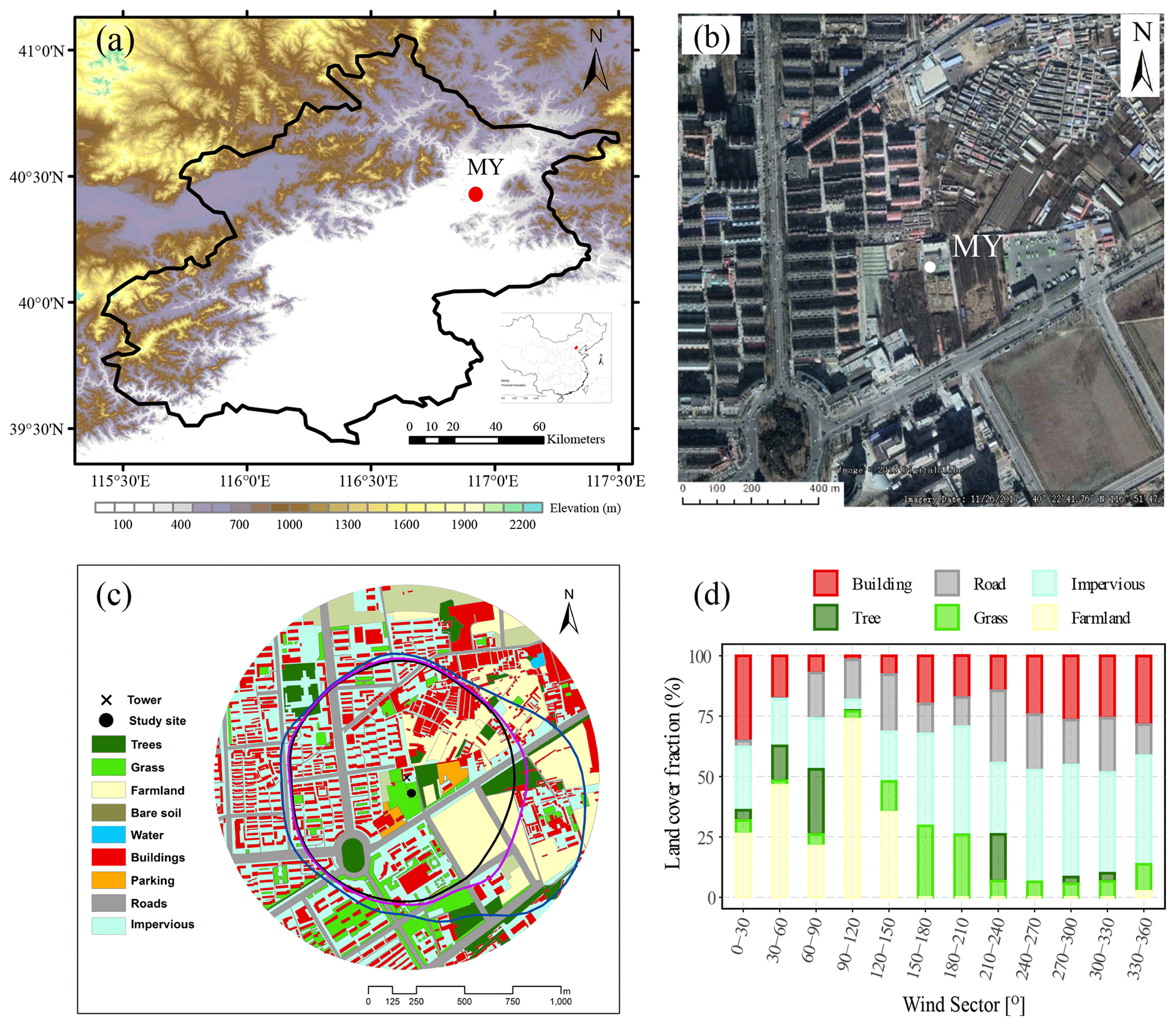
Figure 1 Study area: (a) Beijing topography with Miyun (MY) (inset; location in China, red dot); (b) aerial view around MY flux tower (© Google Earth 2017); (c) land cover within 1 km radius around the MY flux tower (black cross) and 90 % eddy covariance source area for daytime ($K_{\downarrow }>\mathrm{5}$ W m⁻², black line), night (blue), and daily (pink) averages; (d) daily mean land cover derived from a Gaofen-2 high-resolution image (CCRSDA, 2016) for the 30^∘ wind sectors of the 90 % source area (shown in c).

Within a 1 km radius of the Miyun instrumented tower, the surface is 69.6 % impervious (20.6 % buildings, 14.6 % roads, and 34.3 % parking lots and pavement) and 30.3 % vegetation (15 % wheat–maize rotation farmland, 7.2 % trees, 8.1 % grass) based on an analysis of a Gaofen-2 high-resolution image (CCRSDA, 2016) with a spatial resolution of 1 m (Fig. 1c). To the east and southeast of the tower, there is farmland. The mainly residential six-story (∼18 m) buildings are at varying distances (west: from 170 m; northwest: >200 m; north: >70 m) of the tower. Other buildings include the farmer's one- to two-story house (3.5–7.3 m), which is about 300 m northeast of the tower. Since 2016, to the southwest (500-1000 m), newer, taller (18–34 m) residential buildings have been built. To the south (150–500 m away) are office (height: 8–50 m) and light commercial buildings (small shops, 8–12 m). Southwest of the tower, there is a roundabout that connects the two main roads in the study area: the east–west Jingmi Road (170 m to south) and the north–south Tanxi Road (420 m to west).

2.2 Instruments and data processing

Both the eddy covariance (EC) system and radiometer are mounted 36 m above ground level (agl) on a 38 m triangular lattice tower, with the EC system pointing in the prevailing wind direction (east) and the radiometer pointing south to avoid shadows. The EC system's three-dimensional sonic anemometer–thermometer (CSAT3, Campbell Scientific Inc., USA) measures vertical, along-wind, and crosswind velocity and virtual temperature; and the open-path infrared gas analyzer (LI-7500, LI-COR, Inc, USA) measures water vapor and carbon dioxide molar densities. The 10 Hz data are logged on a CR3000 data logger (Campbell Scientific Inc., USA). The 30 min turbulent sensible and latent heat fluxes are obtained using the EddyPro Advanced (v6.1.0 beta, LI-COR) software with standard correction procedures (Moncrieff et al., 1997) applied to ensure data quality (e.g., de-spiking raw data, tilt correction, time-lag compensation, double coordinate rotation, spectral corrections, and Webb et al. (1980) density corrections). Any 30 min period with a poor-quality flag (i.e., 2; LI-COR, 2023; N=1552 (6.6 %) of Q_H and 1987 (8.5 %) of Q_E) is excluded from this analysis. Data are excluded during rain and 2 h after rain (N=615 (1.4 %)). Wind direction data are corrected for changes in magnetic declination as the anemometer was installed with respect to magnetic north.

The radiation fluxes, measured with a CNR4 radiometer (Kipp & Zonen, the Netherlands), are 1 min samples by the CR3000 data logger, from which the 30 min means are calculated. The incoming and outgoing longwave (L_↓ and L_↑) and shortwave (K_↓ and K_↑) radiation and net all-wave radiation (Q^*) data are restricted to physically reasonable thresholds, with nocturnal shortwave radiation forced to 0 W m⁻² (Michel et al., 2008).

On the MY tower four levels (10.0, 17.2, 24.2, 36.0 m) of air temperature and relative humidity (HMP45C, Vaisala, Finland) and wind speed (010C, Met One Instruments, Inc., USA) and two levels (10.0, 36.0 m) of wind direction (020C, Met One Instruments, Inc., USA) are measured.

During the 16-month period analyzed (September 2012–December 2013), after instrument failures (14 January to 18 February 2013), 91.6 % (N=21 416; 30 min periods) of the radiation, 78.9 % (N=18 453) of sensible heat (Q_H), and 77.3 % (N=18 059) of the latent heat flux (Q_E) data are available.

Additional observations analyzed are from an automatic weather station located 30 m from the EC tower. The variables include air temperature (HMP155, Vaisala, Finland) measured at 1.5 m a.g.l.; precipitation from a tipping bucket rain gauge (SL3-1, Shanghai Meteorological Instrument Factory, China) mounted at 0.7 m a.g.l (April to October) and from a weighing bucket rain gauge (DSC1, Aerospace Newsky Technology, China) mounted at 1.5 m a.g.l. (November to March); wind speed and direction (ZQZ-TF, Aerospace Newsky Technology, China) measured at 10 m a.g.l.; and soil temperature (ZQZ-TW, Aerospace Newsky Technology, China) measured at 0, 0.05, 0.10, 0.20, 0.40, 0.80, 1.6, and 3.2 m below ground. These data are sampled at 1 s, except for wind speed and direction (0.25 s), and averaged to 1 min (WUSH-BH, Aerospace Newsky Technology, China). Hourly means (or accumulated totals for precipitation) are used here. Quality control checks include plausible range, internal consistency, temporal and spatial consistency, and other standard China Meteorological Administration network checks (Ren et al., 2015).

Soil moisture content is measured from gravimetric samples collected with a straight-shank drill with a scale. Measurements are taken on the 8th, 18th, and 28th of each month within 300 m of the site between 8 March and 28 November each year at five equally spaced depths (0.1 m interval to 0.5 m) in irrigated cropland and for the natural bare soil at five additional levels (i.e., 10 levels of 0.1 to 1 m).

2.3 Meteorological conditions during the study period

The study period (1 September 2012 to 31 December 2013) is compared to normal (1991–2020) MY weather station data. The range in mean 2 m air temperature is between −13.3 ^∘C (23 December 2012) and 29.4 ^∘C (17 August 2013) at the daily scale and between −7.0 ^∘C (January 2013) to 26.1 ^∘C (July 2013) for monthly scale (Fig. 2a). There are only small deviations from the norm in the monthly mean air temperatures, with the biggest differences (December 2012, April 2013) both 3.1 ^∘C cooler than normal.

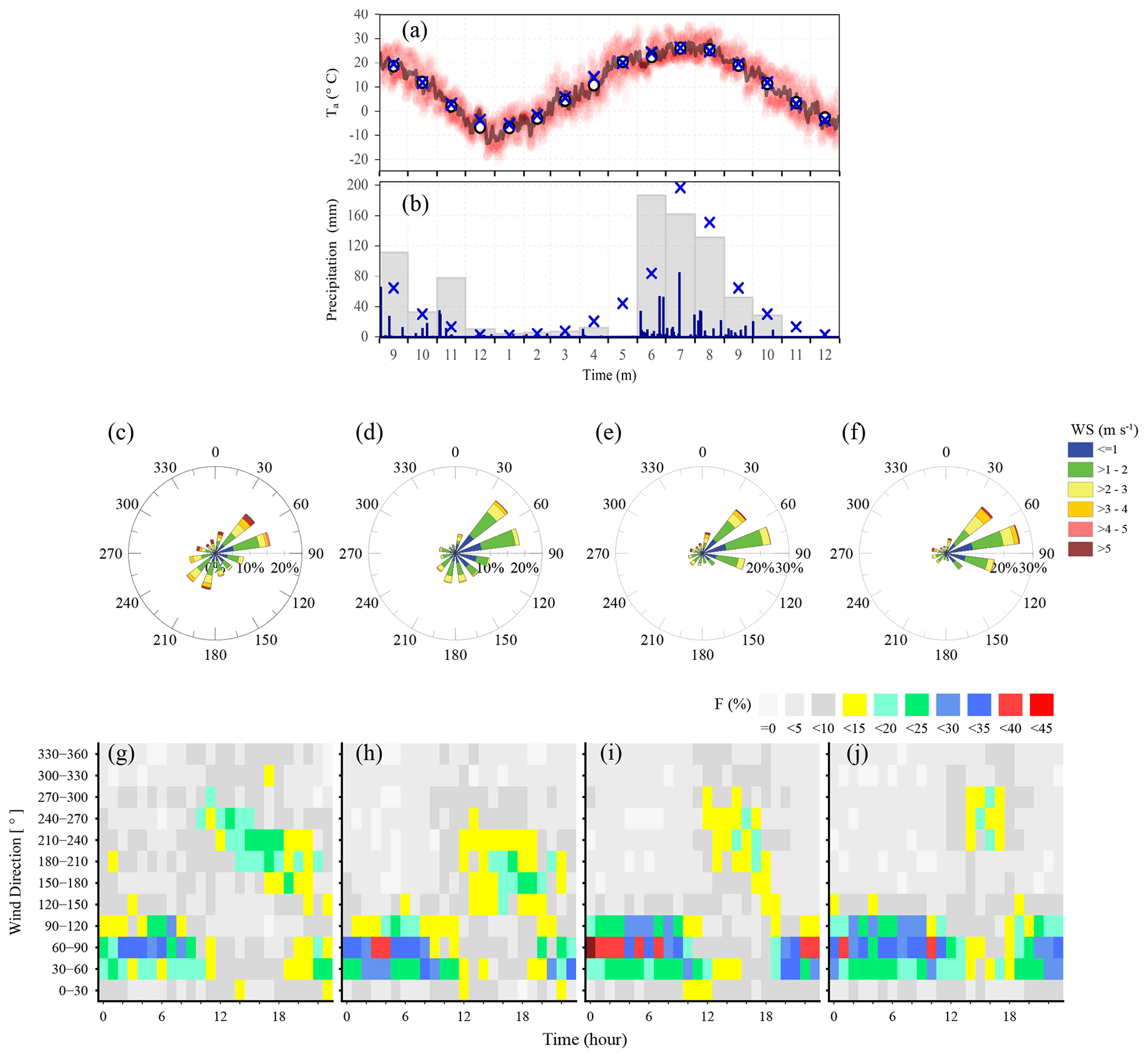
Figure 2 Monthly normal (1991–2020, blue crosses) and automated weather station data (September 2012 to December 2013): (a) 2 m air temperature (T_a ) as 1 h (dots), daily (solid line), monthly averages (white circles); (b) daily (blue), monthly (grey) precipitation; wind roses (30^∘ bins, 1 h data) stratified by wind speed frequency for (c) spring (MAM), (d) summer (JJA), (e) autumn (SON), (f) winter (DJF); frequency distribution of wind direction (30^∘, 1 h data) by time of day for (g) MAM, (h) JJA, (i) SON, and (j) DJF.

The study period precipitation differed significantly from normal conditions in the region (Fig. 2b). The year 2012 was extremely wet, especially on a monthly basis with November (77.4 mm) and December (10.6 mm) about 580 % and 400 % greater than the norm (13.4 mm, November; 2.7 mm, December), respectively. In contrast, most of 2013 had below-average rainfall, except for June, which was wetter (186.7 mm, 223 % of the norm). Notably, dry spells occurred in May, November, and December 2013. Only 0.7 mm (1.6 % of the norm) of rain fell in May, and there was no rain in November and December 2013 at all.

Easterly winds (30–120^∘) prevailed at night and the whole day for every season in MY, with a frequency of 50 % and 38 % in spring, 54 % and 43 % in summer, 69 % and 54 % in autumn, and 72 % and 62 % in winter, respectively (Fig. 2c–j). During the daytime, wind also came from the southwest direction (180–270^∘) because of the mountain–valley breeze, despite the southwest wind differing at the start and end times of the seasons (Fig. 2g–j). In addition, the strongest winds (wind speed > 5 m s⁻¹) mainly came from the northeast (30–60^∘), with a higher relative frequency in spring and winter (Fig. 2c–f).

2.4 EC footprint analyses

To calculate the turbulent flux source areas for each 30 min period, we use the Kljun et al. (2004) EC footprint model. The roughness length for momentum (z₀) and zero plane displacement height (z_d) input parameters is based on the height of roughness elements within a 1 km radius of the EC tower. The buildings vary from 3.0 to 50.4 m. The farmers' houses range from 3.5–7.3 m to the northeast of the tower. The residential buildings (six floors) are to the west, northwest, and north of the tower, with consistent heights of 16.0–18.5 m. The height of buildings to the south, southwest, and north of the tower varies greatly, but most of the buildings exceed 20 m. The tallest building (50.4 m) is 380 m south of the tower. The mean, weighted by the plan area fraction of building height (z_h), is 13.1 m. The trees are along roadsides, within the median strips of roundabouts, public gardens, and orchards (Fig. 1c). The average tree height is 8.5 m (trees > 1.5 m), varying between 5.0–21.0 m with tree species differences. The fruit trees in the orchards (northeast and east of the tower) are a relatively consistent 7.2 to 9.3 m (average = 8.6 m). The mature wheat (June) is 1.1 m and maize (September) is 2.7 m. Using a rule of thumb (Grimmond and Oke, 1999a) with a mean building height of 13.1 m, z₀ is estimated to be 1.3 m and z_d is 9.2 m, whereas using Kanda et al. (2013) for the 36–10^∘ sectors gives values between 0 and 3.26 m (z₀) and between 0 and 36.4 m (z_d). Anemometric estimates are 2.9 m (z₀) and 4.1 m (z_d) (Dou et al., 2019). Given that prevailing wind is from the east (30–150^∘) where vegetation fraction (λ_v) occupies 60 % of the plan area (≤1 km radius of EC tower), anemometric values are used. By using the iterative method suggested by Kent et al. (2017), the impact of these initial values on the probable turbulent flux source dimensions should become insignificant.

The atmospheric stability parameter ($\mathit{\zeta }=(z-z_{\mathrm{d}})/L$) is a function of the Obukhov length (L) obtained from the EC observations, the sensor height (z) and z_d. Here the variation in turbulence is classified as unstable ($\mathit{\zeta }<-\mathrm{0.1}$), neutral ($\left|\mathit{\zeta }\right|\le \mathrm{0.1}$), and stable conditions (ζ>0.1). During the observation period, after quality control (N=17 142; 30 min periods), the stability is predominately either unstable (40.9 %) or stable (42.4 %), with neutral conditions for 16.7 % of the time.

Footprints during unstable and neutral conditions are analyzed together by wind direction (5^∘ sectors) but split into day ($K_{\downarrow }>\mathrm{5}$ W m⁻²) and night. The median 90 % source area extends to 582–677 m (by direction) during the daytime and 596–908 m at night (Fig. 1c), which corresponds to a daily median of 559–676 m. Within these source areas, the land use and land cover vary by sector from being more highly vegetated (30–150^∘) to more built-up (210–360^∘) (Fig. 1d).

2.5 Anthropogenic heat flux

The LQF version (Lindberg et al., 2018; Gabey et al., 2019) of the Large-scale Urban Consumption of energY (LUCY) model (Allen et al., 2011; Lindberg et al., 2013) is used to calculate anthropogenic heat flux (Q_F). The temperature response coefficients are calculated for MY using local air temperature and electricity consumption, vehicle, and population data (Appendix A).

2.6 Storage heat flux

Given the difficulty of measuring the storage heat flux (ΔQ_s) directly in urban areas (e.g., Offerle et al., 2006b; Roberts et al., 2006), we use two methods to estimate it.

1. Objective Hysteresis Model ΔQ_s,ohm: see Appendix B for details.

2. Energy balance residual $\mathrm{\Delta }{Q}_{\mathrm{s},\mathrm{res}}=(Q^{*}+Q_{\mathrm{F}})-(Q_{\mathrm{H}}+Q_{\mathrm{E}})$: includes the uncertainty in other terms in the equation. On the one hand, the EC fluxes (Q_H and Q_E) underestimated by 10 %–20 % (Wilson et al., 2002; Foken, 2008), and on the other hand, given the prevailing easterly winds (30–150^∘) (Fig. 2c–j), vegetation accounts for 60 % of the area of which 44 % is cropland (Fig. 1c and d) if Q_F is included, the ΔQ_s,res values should be regarded as the upper limit of heat storage flux (Ward et al., 2013).

2.7 Data availability and analysis of fluxes

Analysis is done by season (spring: March–May (MAM); summer: JJA; autumn: SON; and winter: DJF) and by time of day (daytime: $K_{\downarrow }>\mathrm{5}$ W m⁻², night: other times).

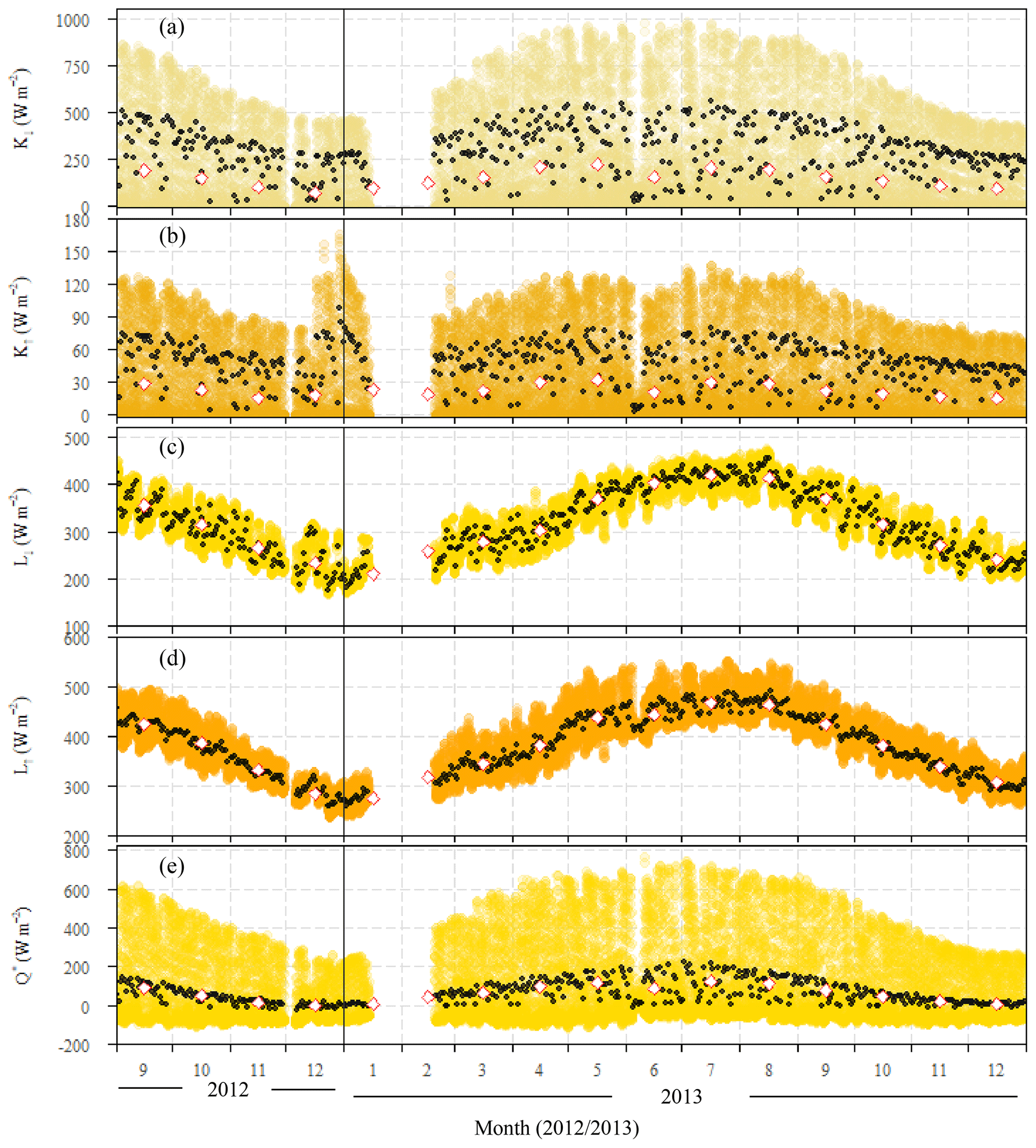
Figure 3 Observed 30 min (color), daily (black), and monthly (white diamonds) means at Miyun (September 2012 to December 2013) of (a) incoming shortwave radiation (K_↓), (b) outgoing shortwave radiation (K_↑), (c) incoming longwave radiation (L_↓), (d) outgoing longwave radiation (L_↑), and (e) net all-wave radiation (Q^*). The data gap in January and February 2013 is due to instrument failure. For the daily fluxes, daytime values ($K_{\downarrow }>\mathrm{5}$ W m⁻²) are given for the shortwave fluxes, but 24 h values are given for the others.

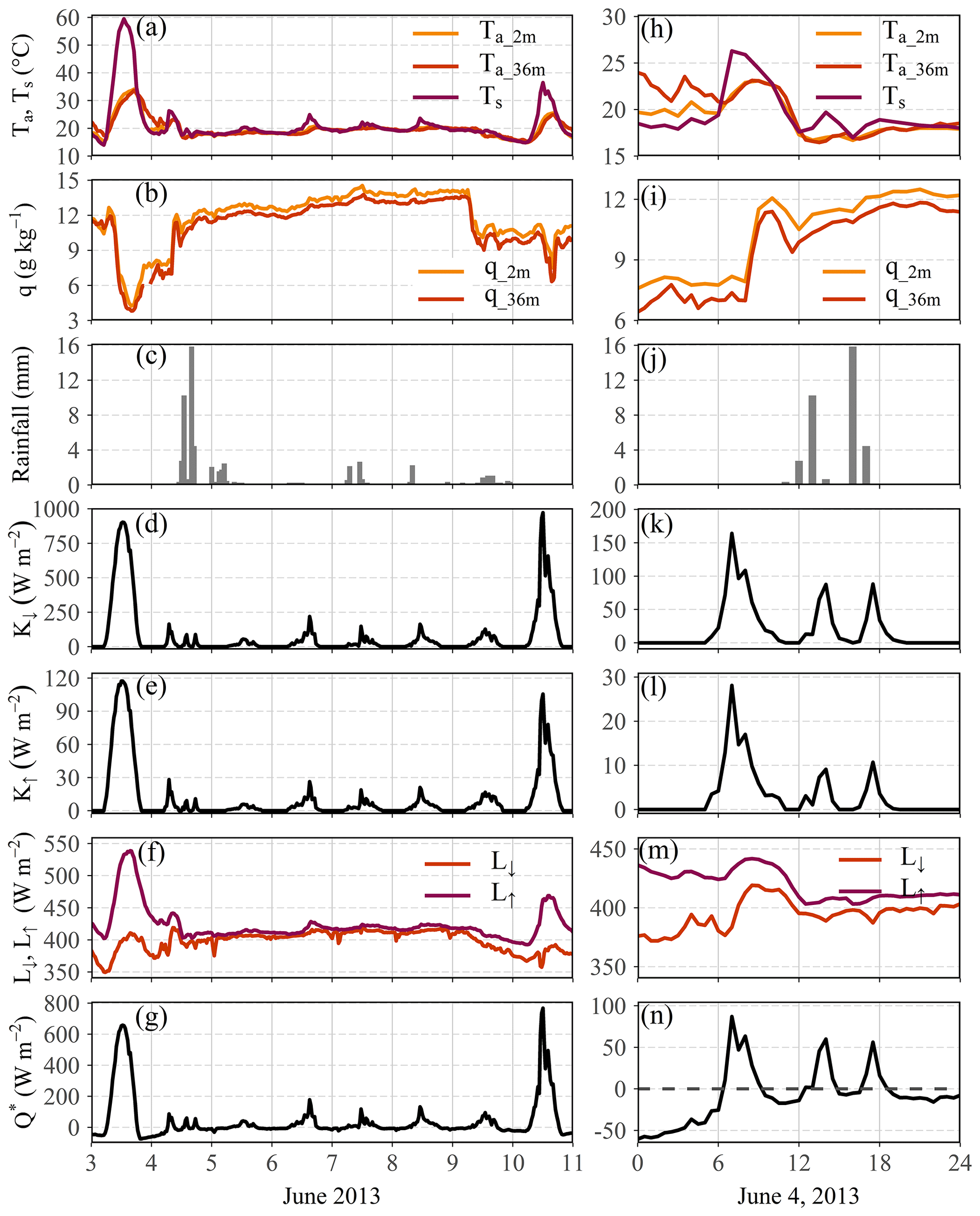
Figure 4 Time series of (a, h) air temperature at 2 and 36 m and surface temperature, (b, i) specific humidity at 2 and 36 m, (c, j) rainfall, (d, k) incoming shortwave radiation, (e, l) outgoing shortwave radiation, (f, m) incoming and outgoing longwave radiation, and (g, n) net radiation for (a–g) 3–10 June 2013 and (h–n) 4 June 2013 at Miyun. Rainfall has a 1 h resolution, and the other data have a 30 min resolution.

Missing data are not gap-filled. The mean values of radiation and turbulent fluxes for each half hour during a day in the month (season) are first calculated to get their mean diurnal patterns. Then the daytime ($K_{\downarrow }>\mathrm{5}$ W m⁻²) or daily (24 h) mean values are averaged from corresponding periods within the mean diurnal patterns. The daytime (daily) mean ratios are the ratios of daytime (daily) mean values of corresponding radiation and energy fluxes.

3 Results and discussion

3.1 Surface radiation budget

At the MY site, daytime maxima of incoming shortwave radiation (K_↓) range from about 500 W m⁻² in winter to 1000 W m⁻² in summer (Fig. 3a). As expected, daytime maxima of K_↓ in winter are greater than those for higher-latitude cities (e.g., London, 52^∘ N, ∼200 W m⁻²; Kotthaus and Grimmond, 2014) and smaller than for lower-latitude cities (e.g., Shanghai, 31.19^∘ N, ∼600 W m⁻²; Ao et al., 2016b), owing to differences in the solar elevation angle. In summer at MY, the daytime maxima of K_↓ is similar to London (Kotthaus and Grimmond, 2014) but slightly higher than for Shanghai (∼800 W m⁻²; Ao et al., 2016b). This may be attributable to the higher humidity reducing K_↓, exceeding the latitudinal differences. The extremely low K_↓ values are associated with precipitation, such as recorded in early June 2013 (Fig. 3a). With rain everyday from 4 to 9 June, the K_↓ maxima were <220 W m⁻² (Fig. 4c and d). K_↓ was 0 W m⁻² between 11:00-12:00 and 16:00 LT on 4 June during rainfall (Fig. 4j and k).

The outgoing reflected shortwave radiation (K_↑) daytime maxima vary between 65 W m⁻² (December) and 120 W m⁻² (July and August). However, some observations in December 2012 and January 2013 exceed 120 W m⁻² and even 150 W m⁻² (Fig. 3b) when snow occurred causing albedo to increase to 0.6 and then decrease with the days since snowfall (Fig. 5). When there is no snow on the ground, an asymmetry in the albedo still exists. With smaller solar elevation, the asymmetry is more pronounced (Fig. S1 in the Supplement). Surface heterogeneity is thought to explain this as there is a basketball court in the field of view of the radiometer (southeast, Fig. S1a), and albedo will differ from impervious and vegetation surfaces in other parts of the field of view (Fig. S1a), including specular reflection from glass. The building with windows is ∼9 m north of the tower, increasing the albedo before noon (cf. afternoon) (Fig. S1b and c). During the spring, summer, and autumn, daily midday (10:00–14:00 LT) albedo was between 0.128 and 0.209 in 2012 (0.113–0.209, 2013), while in winter in 2012 (2013) it reached 0.155–0.478 (0.134–0.293) with the variations in snow cover. Overall, the representative daytime (sunrise to sunset) local-scale albedo was 0.148, which is slightly larger than the midday (10:00–14:00 LT) value (0.145).

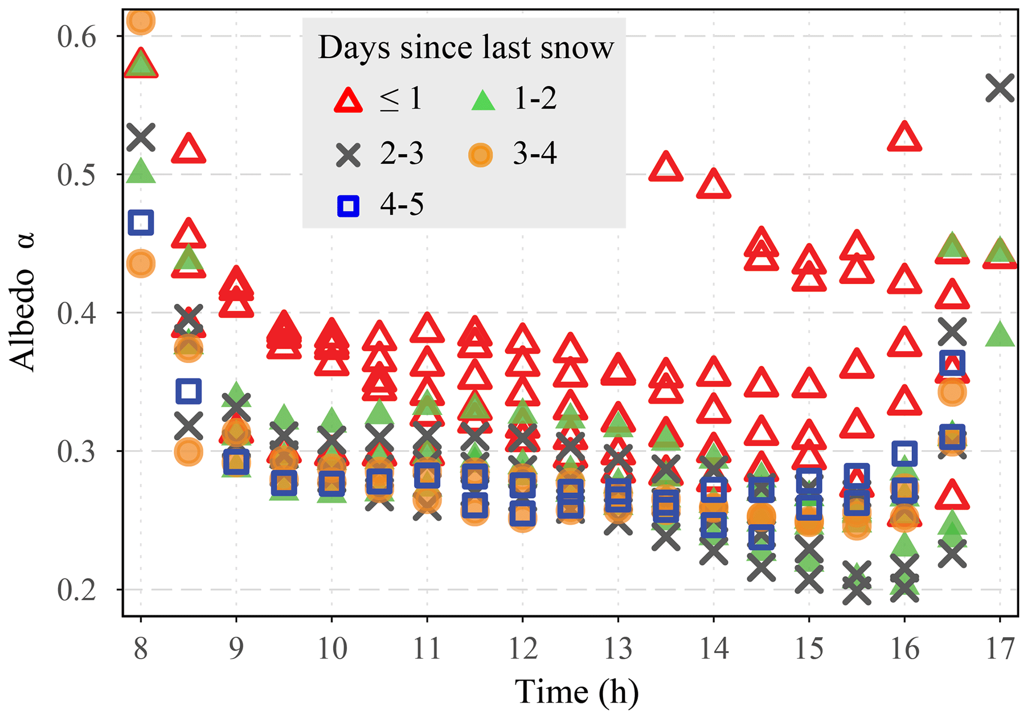
Figure 5 Albedo variation with time since the last snowfall from December 2012 to February 2013.

Incoming longwave radiation (L_↓) is primarily influenced by near-surface air temperature and water vapor content (Flerchinger et al., 2009; Kotthaus and Grimmond, 2014). Thus, the larger L_↓ values are observed during warm and humid times of the year (i.e., summer, June–August) (Fig. 3c), and smaller values are observed in the colder winter. The daily maxima of L_↓ vary between ∼320 W m⁻² (winter) and ∼470 W m⁻² (summer). The monthly mean L_↓ varies between 420 W m⁻² (July) and 212 W m⁻² (January 2013). The latter was the coldest month of the observation period (Sect. 2.3).

Outgoing longwave radiation (L_↑) depends on the surface temperature and emissivity. The former is highly influenced by the total amount of incoming radiative energy. Thus, the larger L_↑ is observed in summer (Fig. 3d), consistent with the larger K_↓ and L_↓. And vice versa, the lowest L_↑, along with smaller K_↓ and L_↓, is measured in winter. The highest monthly mean L_↑ of 467 W m⁻² occurred in July and the smallest (275 W m⁻²) again in January 2013.

As the net all-wave radiation (Q^*) is the net balance of the four radiation budget components, it is affected by sun elevation angle, sky conditions, and surface characteristics. The variation in Q^* is similar to that in K_↓, with daytime maxima of Q^* being greater in summer and smaller in winter. Daily mean Q^* values vary between −20 W m⁻² (winter) and 222 W m⁻² (summer), with large scatter seen from May to September (Fig. 3e). Hence, the largest monthly mean Q^* is in summer, with the maximum value (126 W m⁻²) in July 2013. The smaller monthly mean Q^* in June is attributed to its smaller K_↓ caused by frequent rainfall. Notably, the 4 June's extremely low K_↓ results in a daily mean Q^* that is <0 W m⁻² (Fig. 4n). With longer winter nights the monthly mean Q^* is small or even negative. Notably, the minimum value during the observation period is in December 2012 when snow is present (i.e., decreasing K_↓) resulting in a monthly mean of only −0.5 W m⁻² (Fig. 3e).

3.2 Anthropogenic heat (Q_F) and storage heat (ΔQ_S) fluxes

The median Q_F values vary between 5 and 39 W m⁻² diurnally across all of the months (Fig. 6). Heat released from buildings (Q_F,B) dominated Q_F, with its diurnal median value ranging from 4.6 to 36.4 W m⁻² and accounting for 85 %–95 % of Q_F (Fig. S2a). The contribution of vehicle emission (Q_F,V) is small (1 %–9 % of Q_F). The maximum Q_F,V value during the morning rush hour (08:00–09:00 LT) is only 1.5 W m⁻², since the house is usually close to the work place or school and residents do not rely on cars for daily travel or commuting at MY (Fig. S2b). The diurnal variation in the human metabolism (Q_F,M) is constant throughout a year because of the fixed population density (5657 people km⁻² in 2012 and 5702 people km⁻² in 2013). Like in other studies, Q_F,M is small, with values ranging between 0.4–1 W m⁻² and contributions being 5 %–8 %.

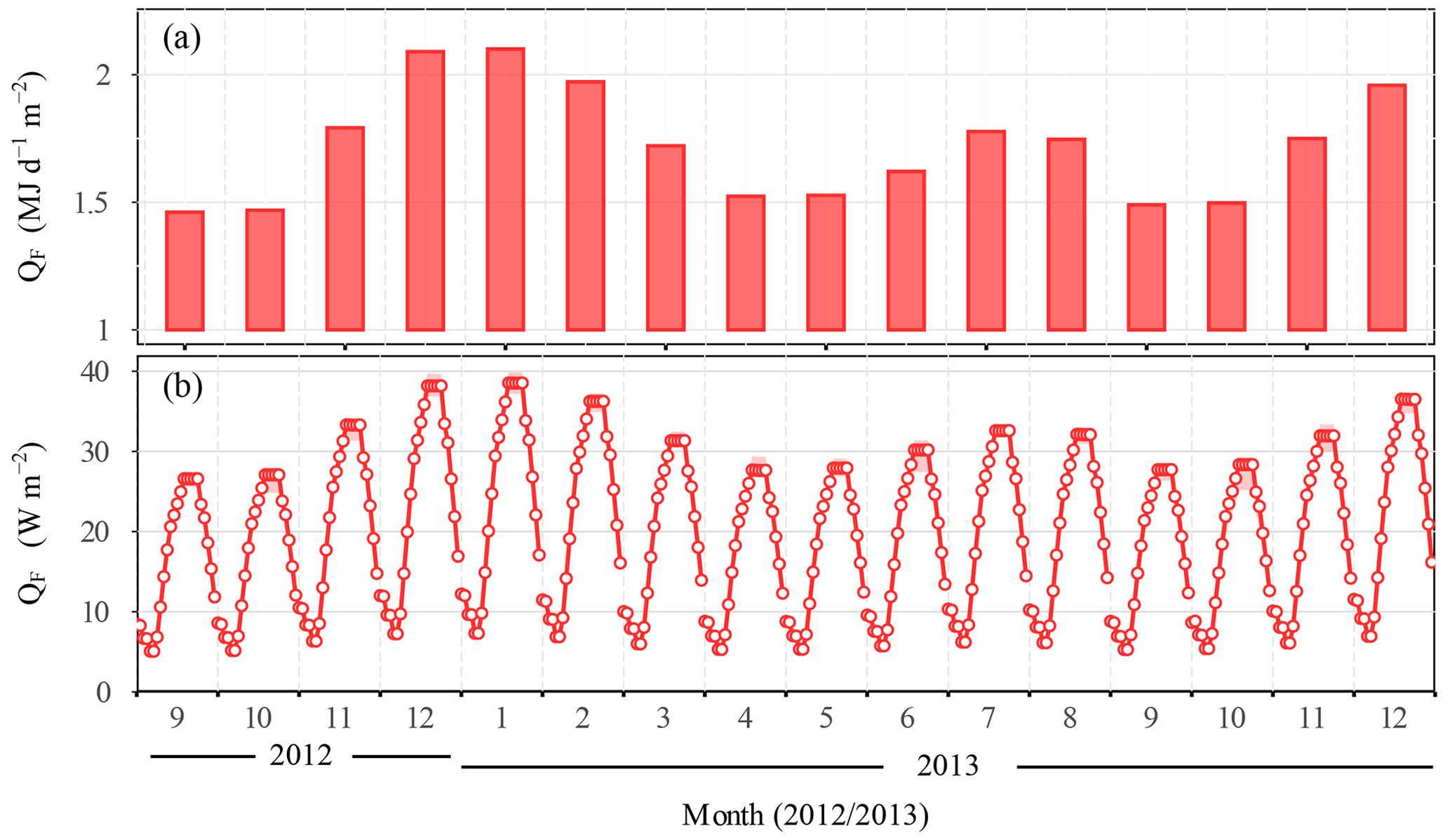
Figure 6 Monthly anthropogenic heat flux (Q_F) at Miyun (September 2012 to December 2013) calculated as described in Sect. 2.2: (a) mean total for 24 h and (b) median diurnal patterns with inter-quartile range (IQR) (shading).

The fluxes are larger in summer and winter associated with cooling and heating needs, respectively. Our Q_F,B values are larger than estimated at other suburban sites, such as Montréal during winter (Bergeron and Strachan, 2012) and Swindon (Ward et al., 2013); even the air temperature in Montréal is lower in winter. The reason is that Miyun has a greater mean building height (13.1 m) and building cover (21 %). Moreover, buildings include hospitals and office buildings, which usually have greater energy consumption and emissions than residential buildings. However, our Q_F,V values are lower than those reported in Montréal and Swindon, due to the small number of motor vehicles and various travel modes at Miyun.

The monthly mean Q_F values vary between 17 and 24 W m⁻² (daily totals = 1.46–2.10 MJ d⁻¹ m⁻²). These suburban values are larger than those reported in other suburban residential areas, such as 10–12 W m⁻² in Montréal during winter (Bergeron and Strachan, 2012) and 6–10 W m⁻² in Swindon (Ward et al., 2013). However, these suburban Beijing values are much less than in Beijing city center (∼130 W m⁻², Wang et al., 2020). Hence, the MY values appear to be reasonable.

The storage heat fluxes are determined using two methods (Sect. 2.6). Generally, storage heat flux is expected to have a net gain in summer and net loss in winter, giving almost zero net heat gain/release over the annual period (Grimmond et al., 1991). From this point of view, ΔQ_s,ohm has a credible annual variation in daily total values (Fig. 7a), but the annual total value of ΔQ_s,ohm was 352.8 MJ m⁻² in 2013, indicating that ΔQ_s,ohm is overestimated.

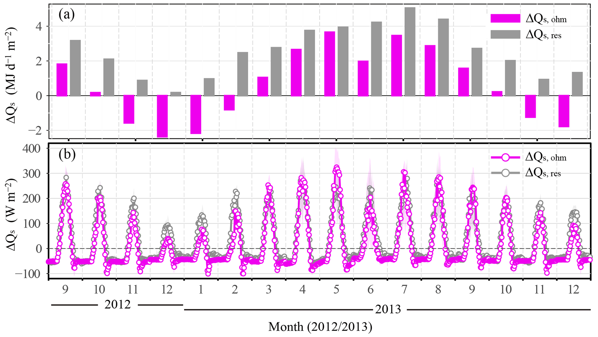
Figure 7 Miyun (September 2012 to December 2013) monthly storage heat flux (ΔQ_S) determined using two methods (color, Sect. 2.5): (a) 24 h mean and (b) diurnal patterns median with inter-quartile range (IQR) (shading).

In spring and summer, there is little difference in daytime values of ΔQ_s,ohm and ΔQ_s,res except for May 2013 (Fig. 7b), indicating an overestimation of ΔQ_s,ohm. The May high ΔQ_s,ohm is the result of both fewer rain events and more radiative input (Sects. 2.3 and 3.1; Figs. 2b and 3a), as it depends on the net radiation value according to the objective hysteresis model (OHM) equation. Meanwhile, farmland irrigation prompts more energy to be used for evaporation (Sect. 3.4 and 3.5; Figs. 14 and 15), resulting in a decrease in ΔQ_s,res. This makes daytime ΔQ_s,ohm obviously higher than ΔQ_s,res in May. In addition, at MY, it is common to see sun after rain in spring and summer, which is similar to pavement/road watering on sunny days. Pavement heat flux (G) is reduced after watering, and the maximum value of G is only half of that without pavement watering under the same sunny conditions (Hendel et al., 2015). However, the OHM coefficients of road/pavement/impervious surface used in this study were fitted from dry surfaces under clear-sky conditions (Anandakumar, 1999; Doll et al., 1985; Wang et al., 2008), so it inevitably leads to an overestimation of ΔQ_s,ohm when it is sunny after rain. The comparison results of a MY daytime ΔQ_s,ohm value greater than ΔQ_s,res within 24 h after rain in spring and summer confirm this point (Fig. S3).

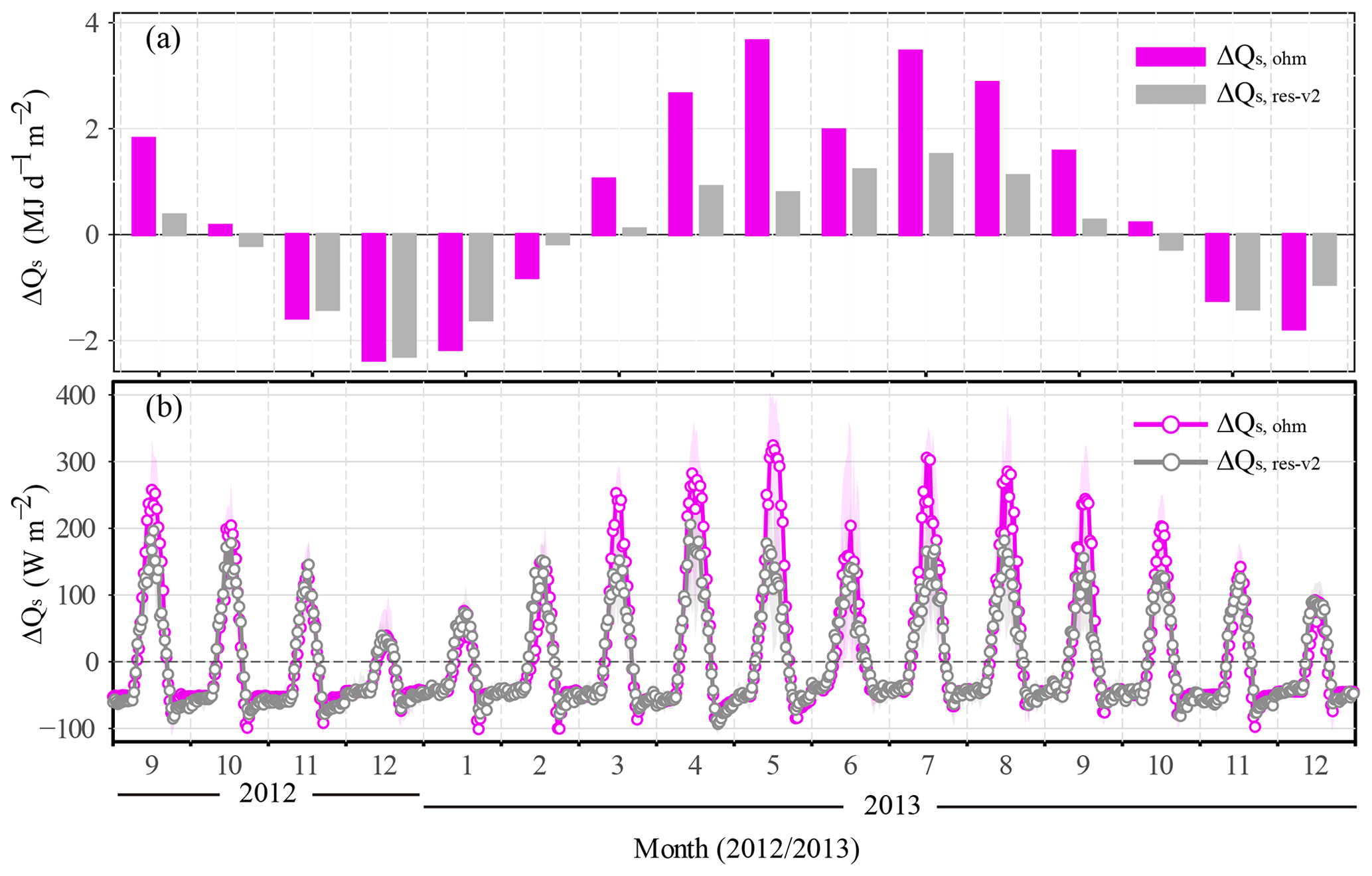
Figure 8 Monthly storage heat flux (ΔQ_S,ohm and ΔQ_S,res-v2) at Miyun (September 2012 to December 2013) (Sect. 3.2): (a) mean flux for 24 h and (b) median diurnal patterns with inter-quartile range (IQR) (shading).

In autumn and winter (November–February), ΔQ_s,ohm is smaller than ΔQ_s,res during the day but larger (more negative) at night (Fig. 7b), similar to residential Swindon results (Ward et al., 2013). As the MY site has greater wintertime Q_F emissions, which directly impact ΔQ_s,res we make a second estimate which omits Q_F and assumes that the turbulent heat fluxes are underestimated by 20 % (Wilson et al., 2002; Foken, 2008) ($\mathrm{\Delta }{Q}_{\text{s,res-v2}}=Q^{*}-\mathrm{1.2}\cdot (Q_{\mathrm{H}}+Q_{\mathrm{E}})$). This gives a lower limit, with ΔQ_s,ohm smaller than ΔQ_s,res-v2 in winter (Fig. 8). This indicates that the winter ΔQ_s,ohm underestimates are related to OHM coefficients for the prevailing wind directions. As cropland covers a greater proportion in the easterly wind direction, it suggests that the wheat coefficients are poor in winter (Fig. B2d). This is because smaller fluxes are obtained from using the soil heat flux (Q_G) data. These relations to Q^* do not account for those components of heat storage fluxes above the soil heat flux plate, such as ground heat storage and biomass heat storage (Meyers and Hollinger, 2004; Oliphant et al., 2004). They constitute an important proportion of the total storage heat flux. Except for cropland and roof surfaces, OHM coefficients of other land cover types are fitted from the spring or summer observation dataset, while these coefficients may not be applicable to autumn and winter and cause the ΔQ_s,ohm to be underestimated in autumn and winter. Long-term datasets covering seasonal changes and surface conditions, especially winter, can provide more OHM coefficients for use (Anandakumar, 1999; Ward et al., 2013).

In addition to the OHM coefficients, mismatching the source area between radiation and turbulent fluxes may also cause the uncertainty in the ΔQ_s,ohm estimation (Fig. S4). ΔQ_s,res is used in the following analyses, but it is clearly biased, as monthly mean daily total values are all positive throughout the year, even in winter (Fig. 7a).

3.3 Monthly diurnal variation in directly observed fluxes

Typically, Q^*, turbulent sensible (Q_H), and latent heat fluxes (Q_E) each have a unimodal distribution in the year but with different seasonal peaks (Fig. 9). Monthly median diurnal maxima of Q^* are higher from April to September, with the maximum value occurring in August, reaching 600 W m⁻². The daytime median maximum Q^* (450 W m⁻²) in June is slightly less than other months during this high-frequency rainfall period. The median diurnal Q^* in December and January is obviously lower than other months, with a peak value of 180 W m⁻² in December 2012 being the minimum value during the observation period. Nighttime Q^* is around −20 W m⁻² during summer and mostly lies between −80 and −60 W m⁻² in other months. Overall, daytime values are greater than nighttime ones during the investigation period except for December 2012 (−0.04 MJ m⁻² d⁻¹), which results in monthly mean daily Q^* having net positive values. These vary between 0.62 and 10.88 MJ m⁻² d⁻¹ (Fig. 9a and b).

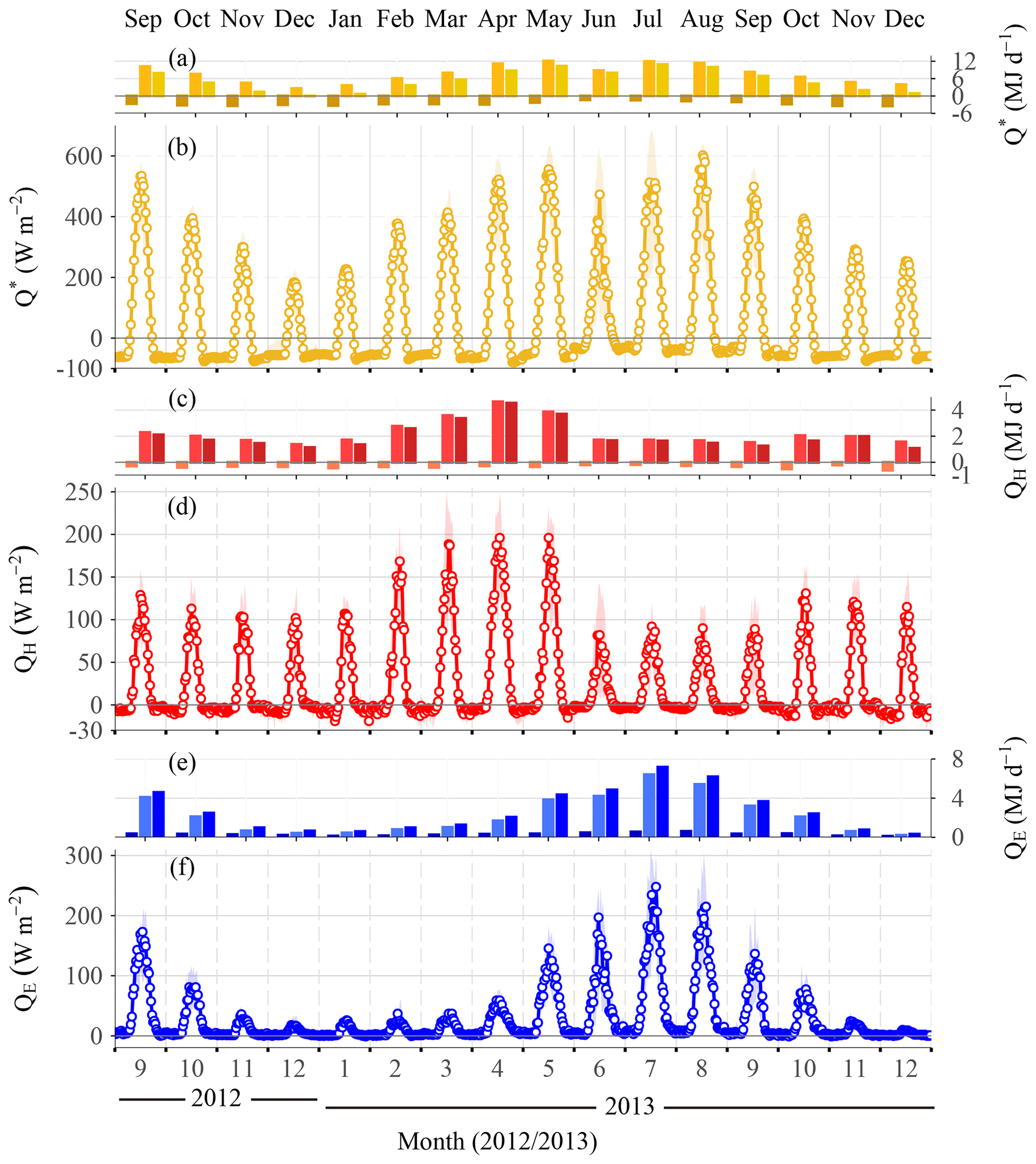
Figure 9 Miyun (September 2012–December 2013) monthly fluxes of (a, c, e) total energy for night, day, and 24 h (left to right) and (b, d, f) diurnal median (line) and IQR (shading) for (a, b) net all-wave radiation Q^*, (c, d) sensible heat flux Q_H, and (e, f) latent heat flux Q_E.

Sensible heat flux Q_H is greatest in spring (March–May) and smallest in June–September 2013 (Fig. 9c and d). The daytime median peak values for these two periods are close to 200 and ∼90 W m⁻², respectively. In other months, daytime Q_H maximum values tend to be of between 100–130 W m⁻², but in February 2013 they approach 170 W m⁻². In previous suburban/urban studies of the East Asian monsoon region, daytime Q_H values are highest in spring (Institute of Atmospheric Physics – IAP, Beijing; Miao et al., 2012; Wang et al., 2015; Xianghe, Beijing, Wang et al., 2015; residential area in Seoul, Hong et al., 2020; Seoul Forest Park, Seoul, Lee et al., 2021) or summer (Tokyo, Moriwaki and Kanda, 2004; Shanghai, Ao et al., 2016a; Osaka, Ando and Ueyama, 2017), depending on whether spring is dry with little rain or warm humidity. Meanwhile, daytime Q_H values are lowest in winter when the least solar radiation in the year occurs, except for Xianghe; Beijing; and Seoul Forest Park, Seoul. Similar to MY, daytime Q_H values of these two sites are lowest in summer, with irrigated cropland/forest within the flux source area. Hence at MY, the summer daytime Q_H minima are attributed to the extensive irrigated cropland in the prevailing wind direction (Figs. 1c, d and 2d, h). This enhances available energy to support evaporation and transpiration and leads to smaller Q_H values (Dou et al., 2019). Notably, these characteristics are different from wheat–maize rotation farmland under the same climate background. The daytime Q_H values in farmland are lowest in spring, owing to sufficient irrigation and high water consumption for wheat growth (Fig. S5). Nocturnal Q_H is negative throughout the year, from a mean of −10.5 W m⁻² in December (2013) to −4.3 W m⁻² in July, which is similar to the values observed at more open suburban sites (Loridan and Grimmond 2012, their Table 2; Oke et al., 2017, their Fig. 6.25). At MY, daily total Q_H values on a monthly basis are smallest in winter, 1.07 MJ m⁻² d⁻¹ in December 2013, and largest in spring (4.53 MJ m⁻² d⁻¹, April 2013) (Fig. 9c). Although the daytime Q_H maxima are smallest in summer, the absolute values at night are smaller than in winter; thus the minimum daily total value occurs in winter.

The seasonal pattern of Q_E is driven by available energy, water supply (including precipitation and irrigation), and phenological variations. Along with the largest Q^* and rainfall, as well as the strongest crop growth in summer, daytime Q_E peaks in July, with the maximum reaching 248 W m⁻² (Fig. 9f). In winter, Q_E is lowest, with median diurnal values < 40 W m⁻². In December 2013, during the long dry spell, with no precipitation from 20 October 2013 (Fig. 2b) and no irrigation (as crops are dormant, typically the last irrigation is before 15 November), the maximum value is only 10 W m⁻². Previous suburban studies report summer and winter daytime Q_E maxima within this range, but at the higher and lower end, respectively (e.g., Grimmond and Oke, 2002; Spronken-Smith, 2002; Christen and Vogt, 2004; Moriwaki and Kanda, 2004; Goldbach and Kuttler, 2012; Dou et al., 2019). Similar to other urban and suburban studies, throughout the day Q_E is positive (Grimmond and Oke, 1995; Balogun et al., 2009; Ward et al., 2013; Ao et al., 2016b). At night Q_E is close to 0, being slightly larger during June–August (between 2–19 W m⁻²; mean 7–26 W m⁻² during 20:00–00:00 LT).

Monthly totals of Q_E are between 0.32 and 7.16 MJ d⁻¹ m⁻² (Fig. 9e), with corresponding maximum and minimum monthly totals occurring in two seasons (summer, i.e., July, and winter, i.e., December 2013, respectively).

3.4 Surface energy balance partitioning

To facilitate the comparison of surface energy balance (SEB) partitioning between sites a series of average daily and daytime ($K_{\downarrow }>\mathrm{5}$ W m⁻²) flux ratios are analyzed. These include fluxes normalized by net all-wave radiation (Q^*) and the Bowen ratio ($\mathit{\beta }=Q_{\mathrm{H}}/Q_{\mathrm{E}}$) (Figs. 10 and 11; Table 1). The ratios are calculated for the 30 min time period, allowing the distributions to be analyzed (Fig. 10), but also using monthly mean fluxes.

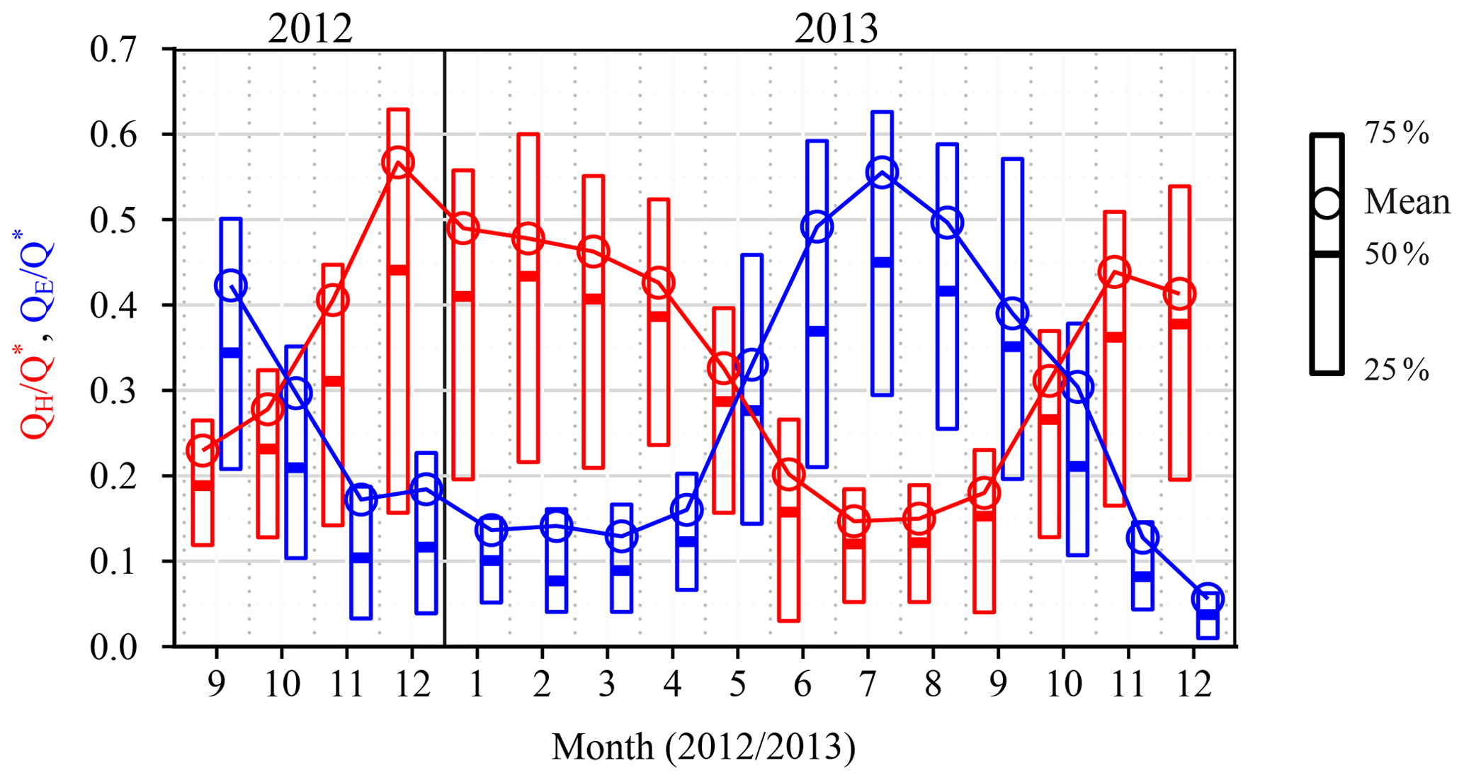
Figure 10 Monthly median, inter-quartile range (IQR) and mean (30 min) of daytime ($K_{\downarrow }>\mathrm{5}$ W m⁻²) sensible heat flux Q_H and latent heat fluxes Q_E normalized by net all-wave radiation (Q^*) at MY (September 2012 to December 2013).

Figure 11 As Fig. 7 but for the Bowen ratio (β) with an inset for May to October 2013.

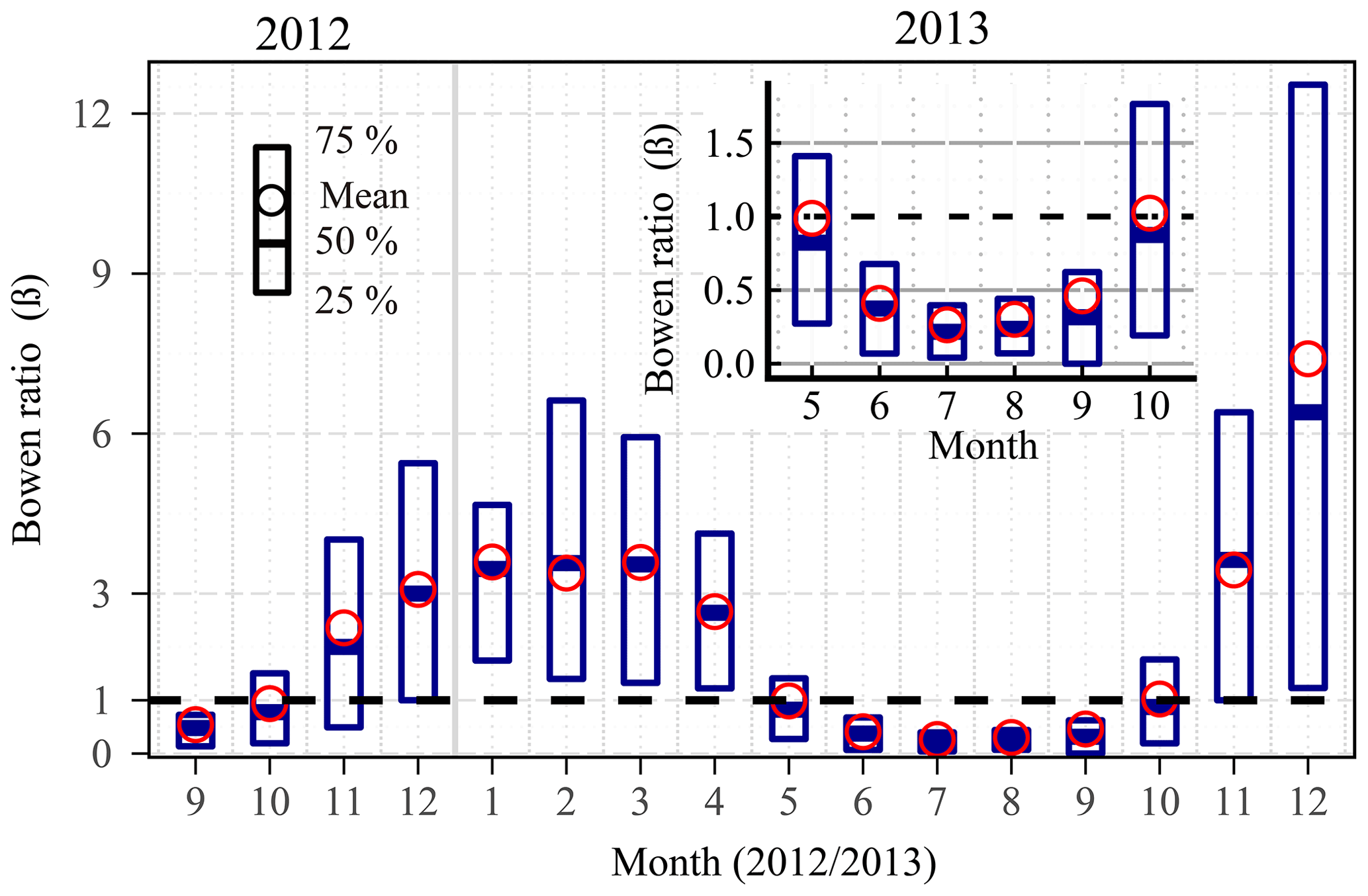
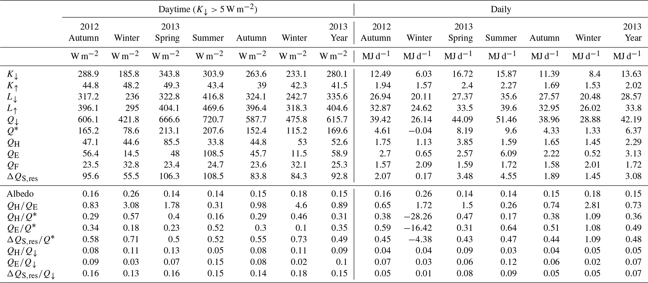
Table 1 Seasonal and annual mean fluxes and ratios for daytime ($K_{\downarrow }>\mathrm{5}$ W m⁻²) and daily (24 h) periods at the Miyun site. The table shows radiation fluxes, net all-wave radiation (Q^*), incoming radiation (Q_↓; $Q_{\downarrow }=K_{\downarrow }+L_{\downarrow }$), incoming and outgoing shortwave radiation (K_↓, K_↑), incoming and outgoing longwave radiation (L_↓ and L_↑), albedo ($K_{\uparrow }/K_{\downarrow })$, turbulent sensible and latent heat fluxes (Q_H, Q_E) and their ratios (radiative ratios; and Bowen ratio ($Q_{\mathrm{H}}/Q_{\mathrm{E}}$), and storage heat flux calculated as $\mathrm{\Delta }{Q}_{\mathrm{S},\mathrm{res}}=(Q^{*}+Q_{\mathrm{F}})-(Q_{\mathrm{H}}+Q_{\mathrm{E}})$. Anthropogenic heat flux Q_F calculated by the LQF version (Gabey et al., 2019; Lindberg et al., 2018) of the LUCY model (Allen et al., 2011; Lindberg et al., 2013).

During the observation period, daytime Q_H is 15 %–57 % of Q^* (Fig. 10). Unlike the absolute values (Sect. 3.3), $Q_{\mathrm{H}}/Q^{*}$ is largest in winter and smallest in summer, whereas $Q_{\mathrm{E}}/Q^{*}$ has the opposite shape with an annual peak in July (Fig. 10). It varies between 6 %–56 % during our study period.

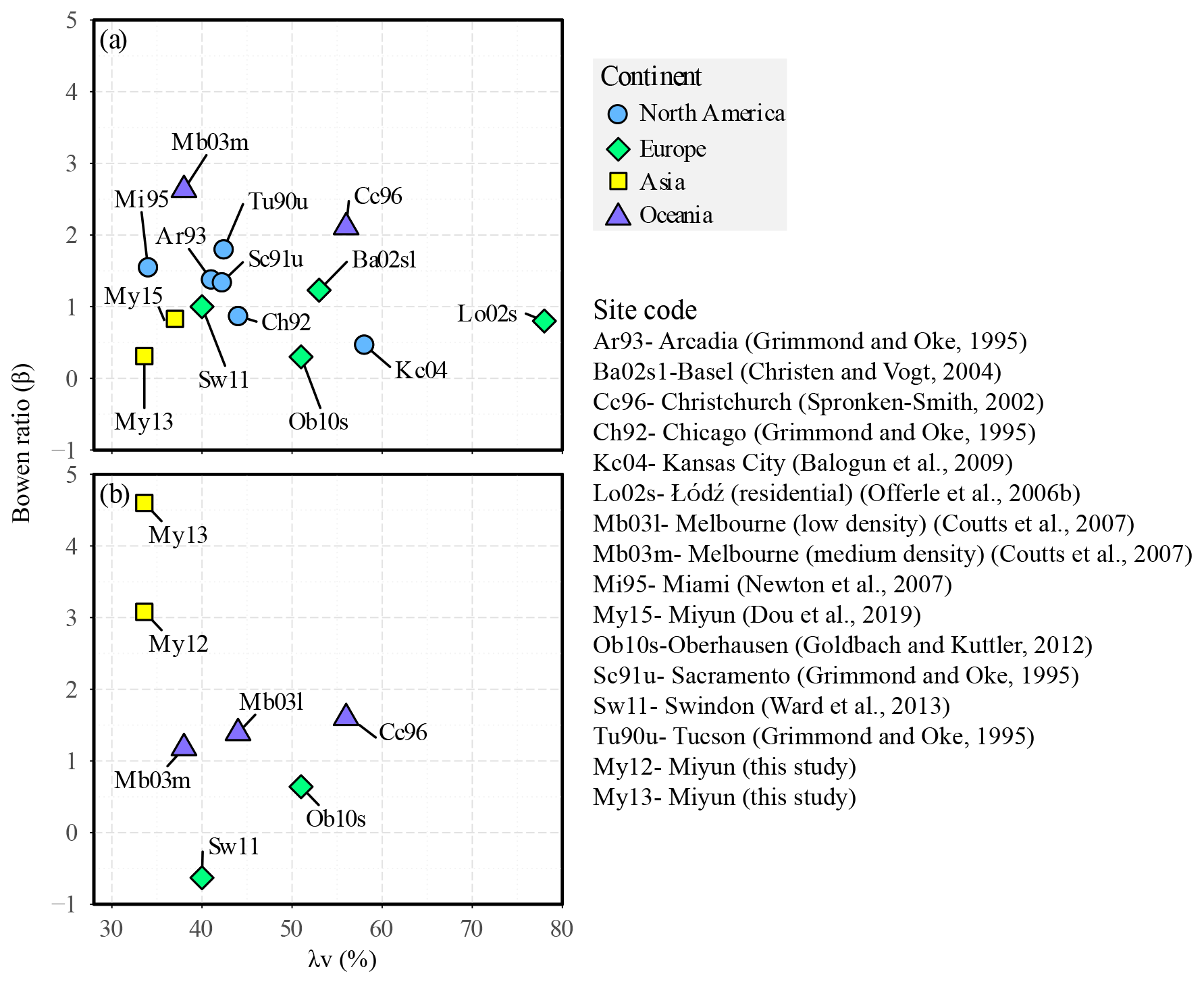
Figure 12 Daytime (the definition of daytime is given in the corresponding publication) Bowen ratio during summer (a) and winter (b) versus vegetation fraction (λ_ν) for MY and for various suburban sites in the literature (see the legend for references).

At MY, from November to April (Fig. 10), Q_H dominates the Q^* ratio, whereas from June to September Q_E dominates the Q^* ratio. For May and October, they have a similar ratio to Q^* (Fig. 10). This partitioning pattern is different from that observed in dense residential Tokyo, where $Q_{\mathrm{H}}/Q^{*}$ is always greater than $Q_{\mathrm{E}}/Q^{*}$ throughout the year (Moriwaki and Kanda, 2004); it is also unlike the pattern reported at a suburban site (Oberhausen), where Q_E is almost always dominant (Goldbach and Kuttler, 2012). These pattern differences could be partly attributed to the different vegetation cover; i.e., λ_V=34 % at MY, 21 % at Tokyo, and 61 % at Oberhausen.

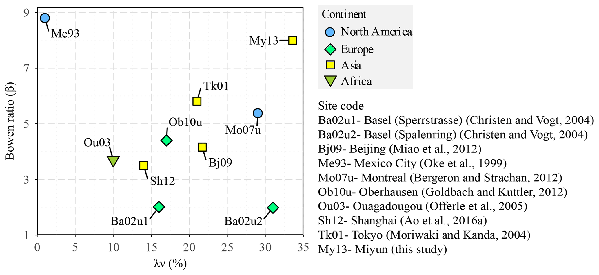
Figure 13 As Fig. 12 but winter daytime Bowen ratio for MY and for various urban sites with a vegetation cover of 1 %–31 %. At Bi09, Ba02u1, Ba02u2, and Sh12, the Bowen ratio is the mean value of December–February. At My13, Me93, and Mo07u, it is the mean value of December. At Ob10u, the value is for January. At Ou03 and TK01, the value is for February. All Bowen ratios are accurately provided in the paper, except for Sh12 extracted from the plot and Mo07u extracted from ratios of $Q_{\mathrm{H}}/(Q^{*}+Q_{\mathrm{F}})$ and $Q_{\mathrm{E}}/(Q^{*}+Q_{\mathrm{F}})$.

The MY June–August daytime $Q_{\mathrm{E}}/Q^{*}$ ratios between 0.49–0.56 (mean summer = 0.52) are greater than at most suburban sites, including those with more vegetation coverage than MY, such as Chicago ($Q_{\mathrm{E}}/Q^{*}=\mathrm{0.38}$; λ_V=44 %; Grimmond and Oke, 1995) and Basel ($Q_{\mathrm{E}}/Q^{*}=\mathrm{0.30}$; λ_V=53 %; Christen and Vogt, 2004). Therefore, MY June–August daytime $Q_{\mathrm{H}}/Q^{*}$ ratios (0.15–0.20; summer mean = 0.16) are lower in comparison to previous studies (Grimmond and Oke, 2002; Balogun et al., 2009; Goldbach and Kuttler, 2012; Dou et al., 2019). Frequent rainfall and irrigation, prevailing winds from farmland, and rapid crop growth are all believed to enhance the latent heat flux, leading to higher $Q_{\mathrm{E}}/Q^{*}$ and smaller Bowen ratio values (Sect. 3.5), and they are consistent with a previous study at the MY (Dou et al., 2019).

In winter, MY daytime Q_H was 41 %–57 % of Q^*, which is greater than at most suburban sites and some urban sites, including sites with larger plan area of buildings (λ_b), such as Tokyo ($Q_{\mathrm{H}}/Q^{*}=\mathrm{35}$ %–40 %; λ_b=33 %; Moriwaki and Kanda, 2004), IAP Beijing ($Q_{\mathrm{H}}/Q^{*}=\mathrm{28}$ %; λ_b=68.3 %; Miao et al., 2012), and Mexico City ($Q_{\mathrm{H}}/Q^{*}=\mathrm{38}$ %; λ_b=32 %; Oke et al., 1999). However, the $Q_{\mathrm{E}}/Q^{*}$ ratios (0.08–0.18) are comparable to those in Tokyo ($Q_{\mathrm{E}}/Q^{*}=\mathrm{0.07}$–0.11; Moriwaki and Kanda, 2004) and slightly larger than that of IAP Beijing ($Q_{\mathrm{E}}/Q^{*}=\mathrm{0.07}$; Miao et al., 2012). This suggests that the higher winter MY $Q_{\mathrm{H}}/Q^{*}$ ratio could be attributed to the relatively lower amount of heat absorbed and stored by buildings (here $\mathrm{\Delta }{Q}_{\mathrm{s}}=Q^{*}-Q_{\mathrm{H}}-Q_{\mathrm{E}}$) due to smaller λ_b (18.9 %). The ΔQ_S is a small proportion of the Q^* energy partitioning ($\mathrm{\Delta }{Q}_{\mathrm{s}}/Q^{*}=\mathrm{0.25}$–0.53).

The partitioning between Q_H and Q_E has clear seasonal variations, with a similar tendency to that of $Q_{\mathrm{H}}/Q^{*}$ (Fig. 11, cf. 10). The daytime β varies between 0.26 and 7.40 through the year (Fig. 11). This range is much greater than at many sites, such as 1.38–5.81 at Tokyo (Moriwaki and Kanda, 2004) and 0.36–1.23 at Oberhausen (Goldbach and Kuttler, 2012). The MY summer and winter (2012 and 2013) daytime mean β values (summer 0.32 and winter 3.08 and 4.60) are at the lower and higher end of those at other suburban sites (Fig. 12). Precipitation plays a significant role in the magnitude and amplitude of β (see Sect. 3.5).

At the annual timescale, Q_H and Q_E are 31 % and 35 % of mean daytime Q^* and 36 % and 49 % of the daily Q^* (i.e., Q_E dominates) (Table 1). Similarly annual, daytime β is 0.89, and daily β is 0.73 (i.e., Q_E dominates).

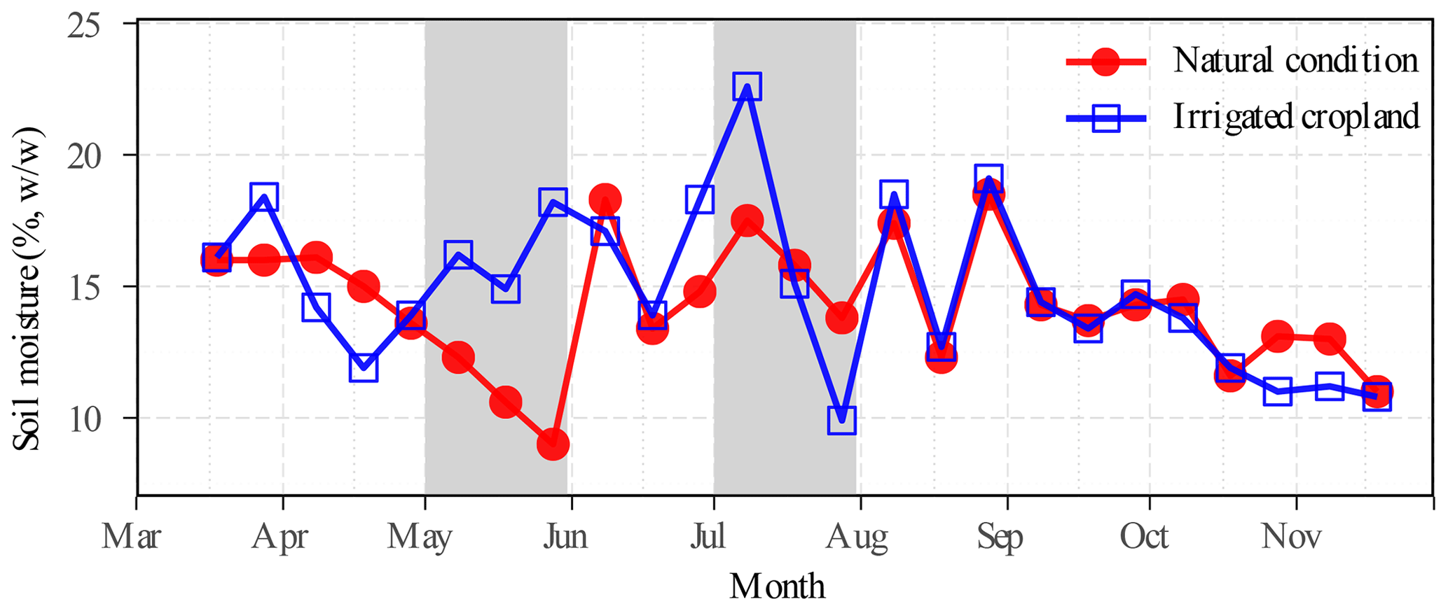
Figure 14 Gravimetric soil moisture (%) at a depth of 0.1 m measured on the 8th, 18th, and 28th of each month at the MY site from 18 March to 18 November 2013 under natural conditions and on irrigated cropland. The shading indicates May and July 2013.

3.5 Factors influencing energy balance fluxes

At MY, the impacts of precipitation on energy partitioning are obvious. As monthly rainfall from September to December in 2012 and 2013 is higher and lower than the norm (1991–2020), respectively, monthly daytime mean β values of September–December 2012 are correspondingly lower than those of the same period in 2013. Notably with no precipitation in November and December 2013, the β in December 2013 reaches 7.40. This is 2.4 times greater than the December 2012 (β=3.08). To our knowledge, this large β value is one of the highest observed not only in suburban areas (Fig. 12b), but also in the central part of cities (Fig. 13), but it is still less than the values observed in central London (β=5–10; Kotthaus and Grimmond, 2014) or Mexico City (β=8.8; Oke et al., 1999).

Irrigation supplements precipitation and plays an important role in energy partitioning (Grimmond and Oke, 1986; Grimmond et al., 1996; Kokkonen et al., 2018). At MY, winter wheat and summer maize are the two predominant crops and are cultivated in rotation. The growing season of winter wheat is from October to mid-June, while maize is planted in late June and harvested at the end of September every year. June and October are the intermittent months for the two crops. Irrigation is frequent during wheat growth in spring because of the drought and climatic conditions with little rain. As shown in Fig. 14, the soil moisture of natural conditions and cropland was almost the same at the end of April (28 April). With only 3 d (26, 27, and 28 May with 0.1, 0.4, and 0.2 mm, respectively) having rain in May 2013 (Fig. 2b), the soil moisture due to natural conditions decreases dramatically in May, whereas, by contrast, that of cropland increases. This indicates that cropland has irrigation to replenish water. For this reason, the May β value clearly presents a decreasing tendency even if there are more than 20 d of no rain (Fig. 15), as external water provided by cropland irrigation makes the available energy favor the latent heat flux. The monthly mean β of 0.50 in May (Fig. 11) clearly indicates the importance of this additional source of water.

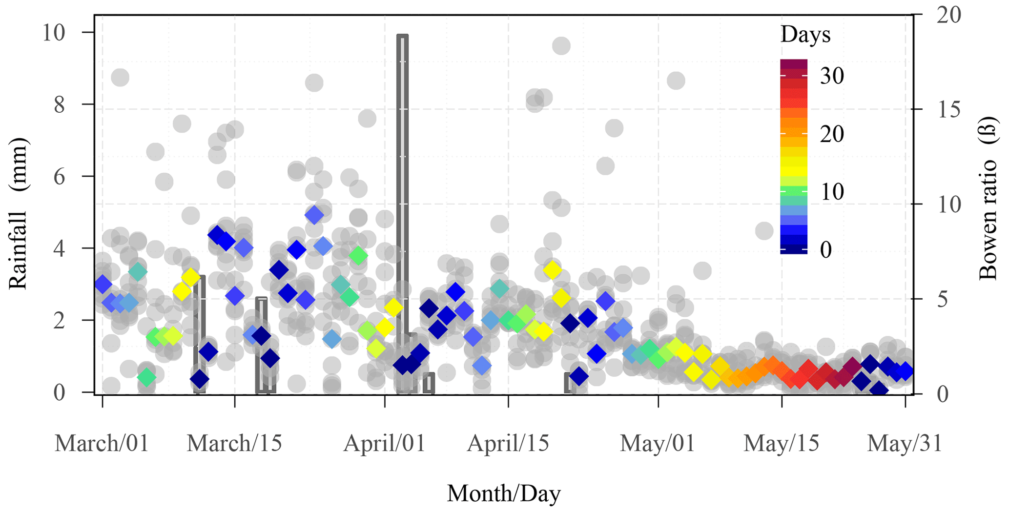
Figure 15 Daytime (circles) and median 30 min daytime (diamonds) Bowen ratio by number of days since rainfall (colors) (right-hand axis) and daily rainfall (bars, left-hand axis) for 1 March to 31 May 2013.

Crop growth and phenology are also important influences. Transpiration during crop growth releases a large amount of water into the atmosphere observed as Q_E (e.g., Dou et al., 2019). The soil moisture in the irrigated cropland is higher than in the natural rainfed areas (Fig. 14). The gravimetric sample dates are critical relative to the timing of both irrigation and rainfall (e.g., 8 July 2013 compared to a few days later) as the soil moisture values can be inverted, as cropland utilizes stored soil water via transpiration and evaporation.

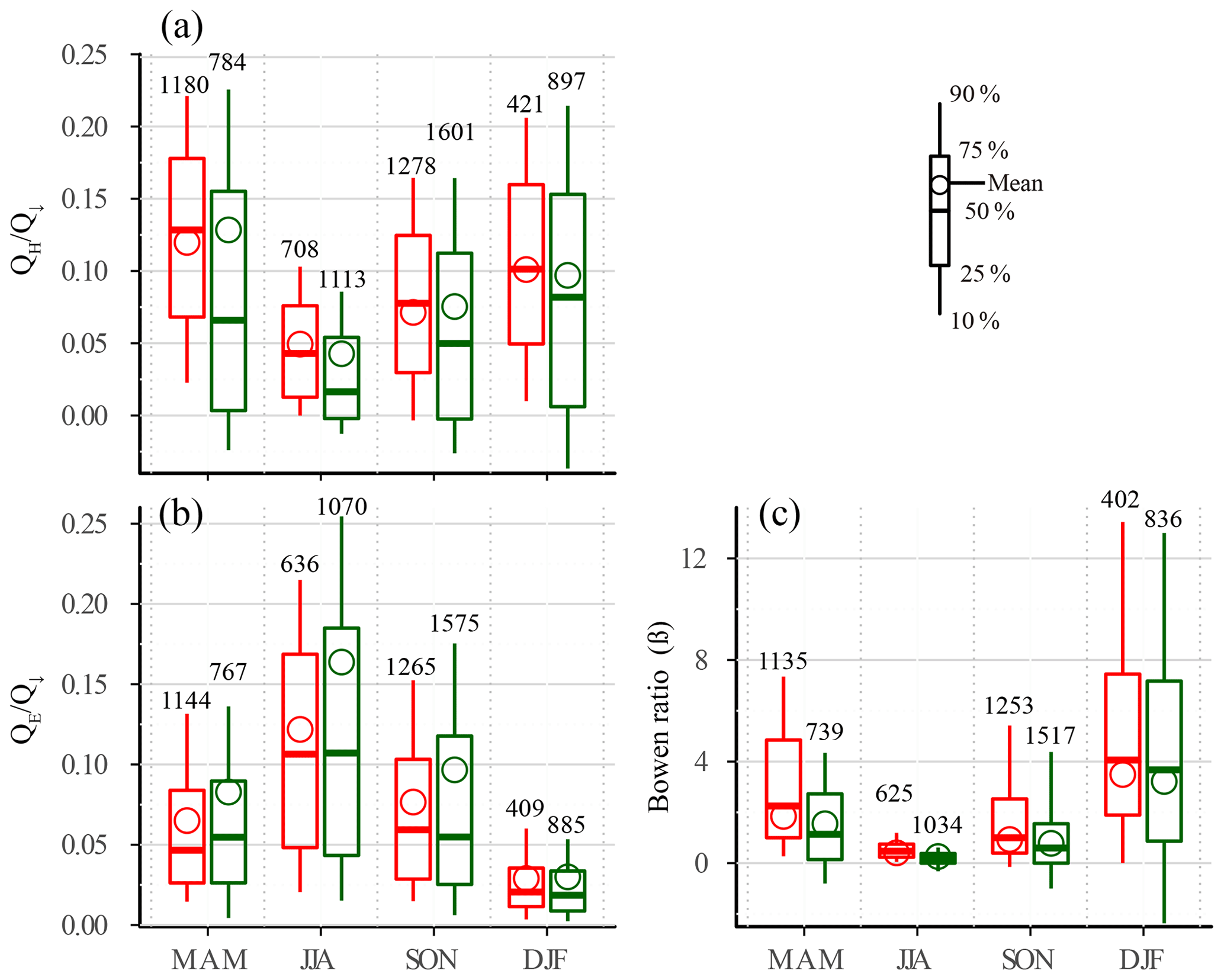
Figure 16 Median, inter-quartile range (IQR), and mean flux ratio (30 min, number of periods indicated) by season when the wind is from the building- (red) and farmland-dominated (dark green) directions. (a) $Q_{\mathrm{H}}/Q_{\downarrow }$, (b) $Q_{\mathrm{E}}/Q_{\downarrow }$, and (c) β (see Table 1 for definitions).

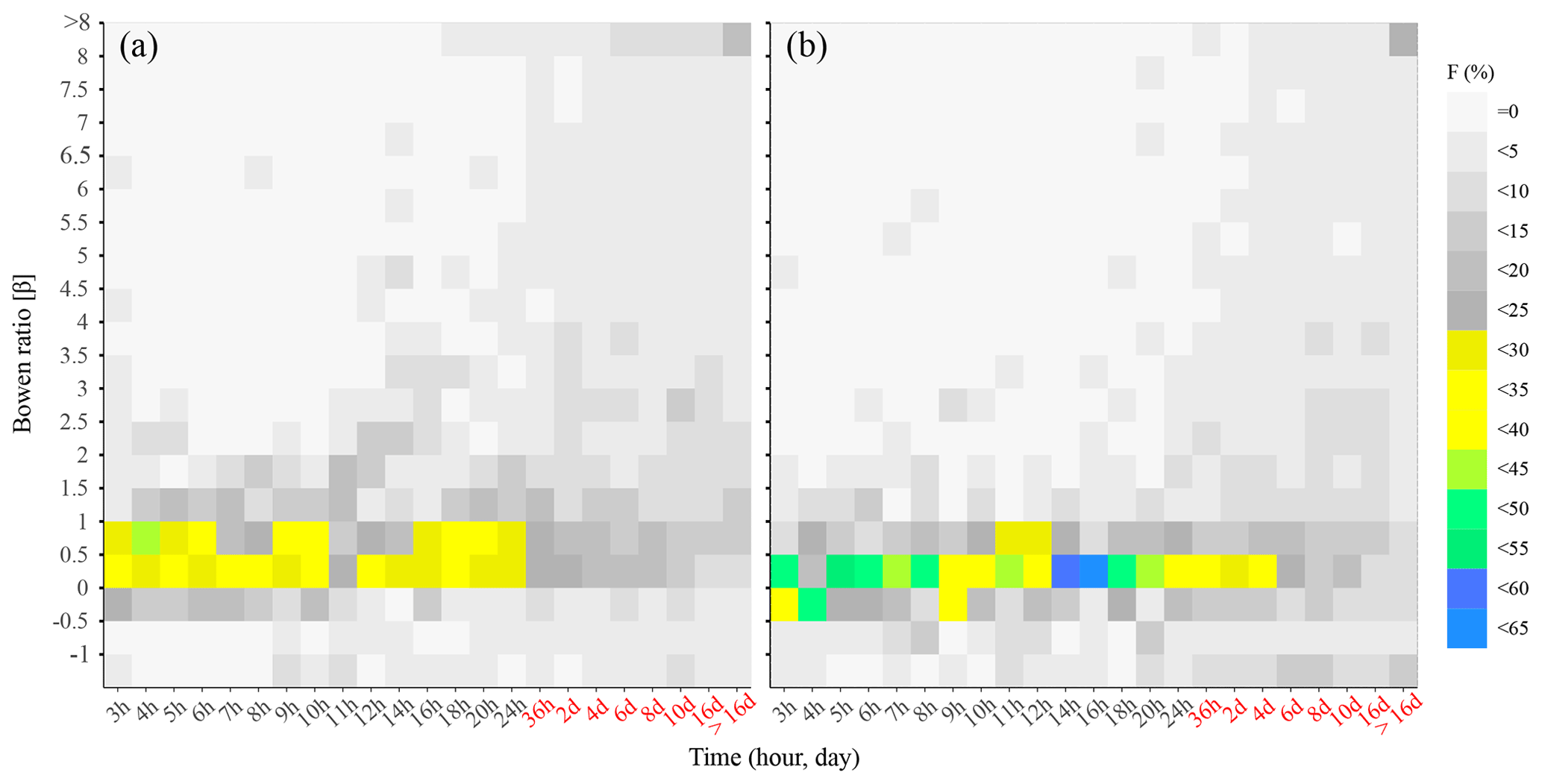
Figure 17 Frequency (F, %) of Bowen ratio β values by time since the last rainfall for (a) building-dominated (210–360^∘) and (b) farmland-dominated (30–150^∘) directions.

In addition to these factors, land use and land cover also play a critical role in the energy budget. As the daily averaged source area is mainly covered by vegetation (60 %) and impervious surface (87 %) in the 30–150 and 210–360^∘ sectors of the tower, respectively, and farmland and buildings are separately the most representative land use and land cover types in the two sectors, observed data from these two sectors are selected to compare energy flux ratios and are accordingly referred to as from farmland- and building-dominated directions. At MY, normalizing measurements by the incoming radiation ($Q_{\downarrow }=K_{\downarrow }+L_{\downarrow }$) the $Q_{\mathrm{H}}/Q_{\downarrow }$ and β ($Q_{\mathrm{E}}/Q_{\downarrow }$) are always more (less) when the wind is from directions with more buildings (cf. cropland-dominated) irrespective of season (Fig. 16). Compared to impervious surfaces, the cropland surface obviously changes between “dry” and “wet” more frequently and with a longer transition time, due to cropland irrigation and water storage by soil. This results in a greater amplitude of $Q_{\mathrm{H}}/Q_{\downarrow }$ and $Q_{\mathrm{E}}/Q_{\downarrow }$ from the cropland-dominated direction. The inter-quartile range and the differences between the mean and median of ratios are clearly greater from the cropland direction (Fig. 16). The temporal variations in β after rainfall differ between these two direction types (Fig. 17). Water can drain relatively quickly after rain in the building-dominated direction because of the high proportion of impervious surface, whereas water can infiltrate into the soil (i.e., it is stored), so β can remain near 1 for longer periods after rainfall (Fig. 17).

4 Conclusions

In this analysis of surface energy flux measurements for a suburb (MY) of Beijing over 16 months we gain a better understanding of surface–atmosphere dynamics.

All components of the radiation balance and net radiation (K_↓, K_↑, L_↓, L_↑, Q^*) have unimodal annual patterns, with higher values in summer (lower in winter) and with the maximum monthly means in July (minima December/January).

At MY, the daytime sensible heat flux Q_H is greatest in spring. However, it is smallest in summer rather than winter, unlike in previous suburban studies. This is because, in the prevailing wind direction, there are extensive cropland, irrigation, and frequent rainfall in summer. All of these factors are thought to play a role. Nocturnal Q_H is negative throughout the year and smaller in winter, so the minimum daily total Q_H still occurs in winter.

The latent heat flux Q_E is positive throughout the day. The daytime maximum Q_E is greatest in summer (July; lowest in winter December) because of the influence of rainfall, irrigation, plant growth activity, and available energy. Monthly median diurnal maxima of Q_E vary from 10–248 W m⁻² during measurement period. These are close to both the smallest and largest values reported for suburban areas. The maximum monthly mean daily total Q_E is in summer (July 2013), and the minimum is in winter (December 2013).

Daytime $Q_{\mathrm{H}}/Q^{*}$ is lower in summer (higher in winter). Across the year it varies from 15 %–57 %. $Q_{\mathrm{E}}/Q^{*}$ has the opposite seasonal trends but a similar annual range (6 %–56 %). Summer daytime means of Q_HQ^* (0.16) are lower and those of $Q_{\mathrm{E}}/Q^{*}$ (0.52) higher than that reported in most suburban areas. In winter daytime $Q_{\mathrm{H}}/Q^{*}$ (0.41–0.57) is greater than reported for most suburban sites, but $Q_{\mathrm{E}}/Q^{*}$ (0.08 to 0.18) is similar to other suburban sites. Thus the storage heat flux ΔQ_S at MY is a small fraction of Q^* because of the low building fraction. At an annual timescale, daytime $Q_{\mathrm{H}}/Q^{*}$ (31 %) and $Q_{\mathrm{E}}/Q^{*}$ (35 %) are very similar, but for the whole day the proportions are 36% and 49 %, respectively.

The large seasonal differences in precipitation and irrigation lead to a wide range in Bowen ratio (β) values across the year (0.26–7.40). Daytime mean β values in summer (0.32) are lower than in winter (4.60) and are at the lower and higher end of the range in the literature for suburban sites. The annual mean daytime β is 0.89 and the daily value is 0.73; thus Q_E dominates available energy.

The results confirm the combined importance of precipitation, irrigation, vegetation growth, and land cover as being key factors affecting energy partitioning in MY. These findings will help to enhance the understanding of the surface–atmosphere energy exchange over Chinese suburban areas, provide observational data for model verification and parameterization scheme improvement, and be a reference for formulating policies to mitigate the adverse effects of urban climate and climate change.

Appendix A: Anthropogenic heat flux estimation

LQF provides a method to calculate anthropogenic heat flux Q_F (Gabey et al., 2019) based on population, vehicle, energy consumption, and air temperature data. It estimates heat released from buildings (Q_F,B), traffic (Q_F,V), and the human metabolism (Q_F,M) (Allen et al., 2011; Lindberg et al., 2013). In this study, we determine an appropriate temperature response coefficient for the MY area.

A1 Temperature response coefficient

In LQF, the mathematical expression of Q_F,B is as follows:

$$\begin{array}{}\text{(A1)}& Q_{\mathrm{F},\mathrm{B}}={\mathit{\rho }}_{\mathrm{pop}}{f}_{\mathrm{b}}{E}_{\mathrm{B},\mathrm{b}},\end{array}$$

where ρ_pop is the population density (people ha⁻¹) and E_B,b is daily building energy consumption (kWh d⁻¹ per capita). The latter, from daily electricity consumption data, accounts for 16 % of the total energy consumption in MY (Table A1).

The coefficient, f_b captures the air temperature response to energy consumption. Given large differences in energy consumption between countries and between cities (e.g., Lindberg et al., 2013), it is preferable to determine the appropriate local f_b as it plays a critical role in building anthropogenic heat emissions. Here f_b varies with air temperature T_a:

$$\begin{array}{}\text{(A2)}& \begin{array}{ll}{f}_{\mathrm{b}}=C+A_{\mathrm{c}}\left(T_{\mathrm{a}}-T_{\mathrm{b}}\right)& T_{\mathrm{b}}<T_{\mathrm{a}}<T_{\max }\\ f_{\mathrm{b}}=C& T_{\mathrm{a}}=T_{\mathrm{b}}\\ f_{\mathrm{b}}=C+A_{\mathrm{h}}\left(T_{\mathrm{b}}-T_{\mathrm{a}}\right)& T_{\min }<T_{\mathrm{a}}<T_{\mathrm{b}}.\end{array}\end{array}$$

Several key parameters to determine f_b are shown in Fig. A1. Here T_b is the air temperature when the energy consumption is the lowest. If the air temperature is higher (lower) than T_b, more energy will be consumed due to cooling (heating). A_c (A_h) is the building energy consumption thermal response slope for cooling when air temperature is above (below) T_b, also known as a cooling (heating) coefficient. C is the minimum energy consumption. T_max and T_min are threshold values for air temperature. When air temperature is beyond this range, energy consumption has reached saturation and no longer increases with air temperature changes.

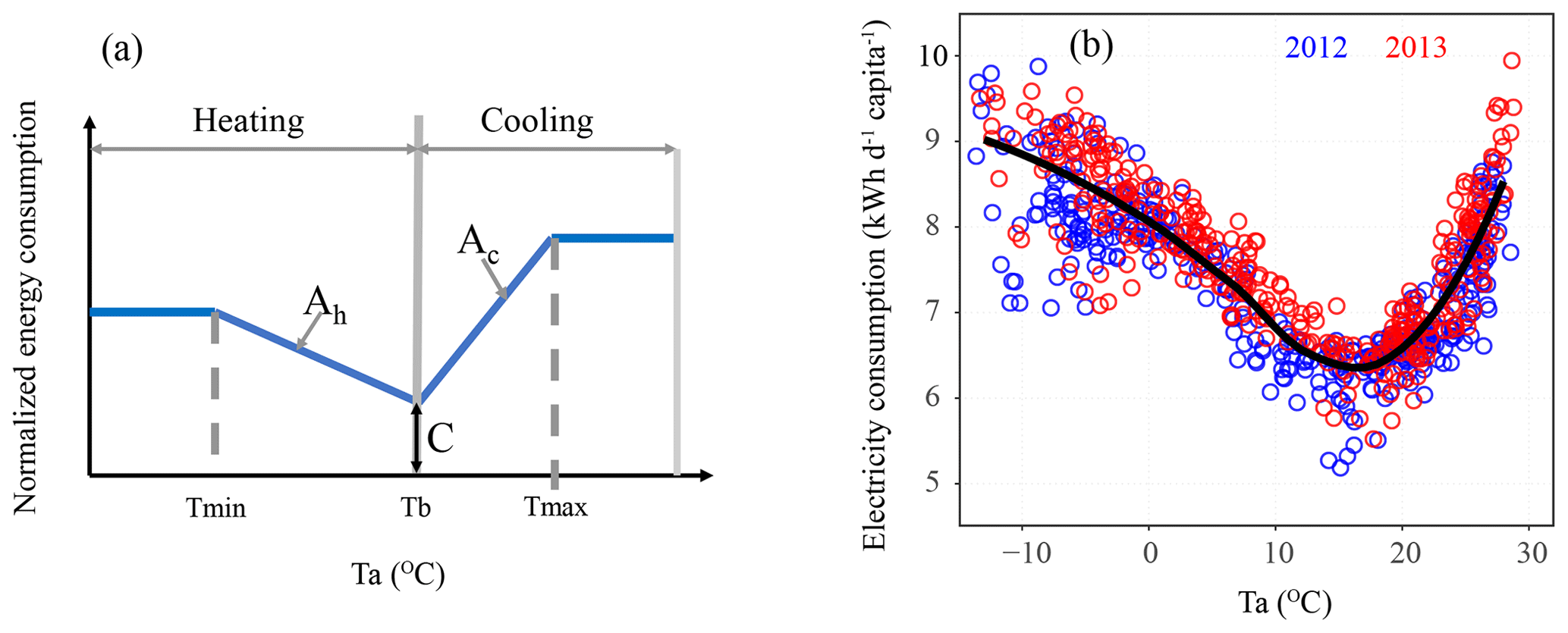
Figure A1 Energy consumption response to air temperature: (a) general response function (see text for definitions) and (b) data for Miyun District (Miyun District daily electricity consumption; kWh d⁻¹ per capita; State Grid Beijing Electric Power Company, http://www.bj.sgcc.com.cn/, last access: 10 October 2023), normalized by population (245 people km⁻² in 2012 and 246 people km⁻² in 2013; Miyun District Bureau of Statistics, 2013, 2014), and MY daily mean air temperature (T_a) for 2012–2013 with the general trend (black, local polynomial regression fitting – LOESS).

Table A1 Energy consumption in Miyun (Miyun District Bureau of Statistics, 2013, 2014) in tons of coal equivalent (TCE) is converted to kilowatt hours assuming 1 TCE = 8141 kWh (Kyle's Converter, 2017).

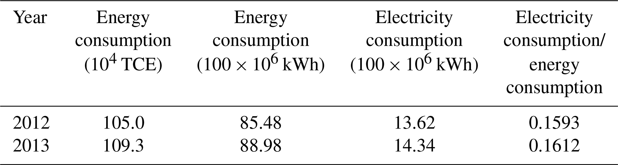
Table A2 Parameters of energy consumption response to air temperature (Eq. A2).

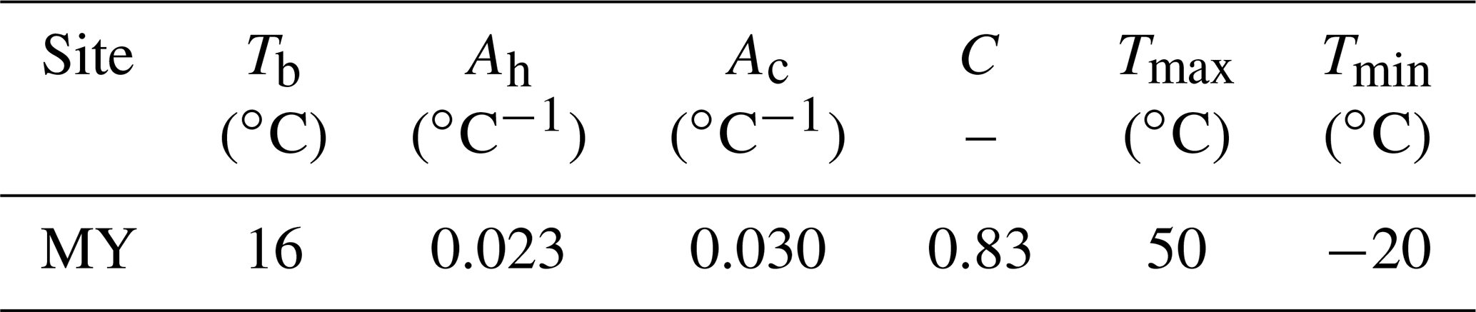
A new set of temperature response parameters applicable to this region is obtained by using daily air temperature and electricity consumption data for the Miyun district in 2012–2013 (Table A1). The resulting parameters are given in Table A2. The energy consumption response to temperature changes is a V-shaped curve in Miyun rather than a U shape as seen in Shanghai City (Ao et al., 2018). The cooling coefficient A_c in MY is lower than that in Shanghai City (0.04 ^∘C⁻¹), which is attributed to relatively short-period air conditioning in MY given the cooler summer nights caused by topography and the continental monsoon climate. However, in winter with colder air temperatures and a longer heating period, the heating coefficient A_h for MY is higher than for Shanghai (A_h=0.01 ^∘C⁻¹) (Ao et al., 2018).

A2 Vehicle numbers

In LQF, Q_F,V is calculated as a function of vehicle numbers, traffic speed, and time (Ao et al., 2018). The average Beijing vehicle numbers per 1000 capita in 2012 and 2013 (245 people km⁻² in 2012 and 246 people km⁻² in 2013; Miyun District Bureau of Statistics, 2013; 2014) are 196.9 and 201.7 cars, 11.7 and 11.7 motorcycles, and 42.6 and 43.7 freight vehicles. For all vehicles the following is assumed: an average vehicle speed of 48 km h⁻¹ and petrol as fuel. Diurnal variation in vehicle numbers for weekdays, weekends, and holidays for Shanghai (Ao et al., 2018) is used as no such data are available for Miyun or Beijing. This will cause additional uncertainties. Given that the Q_F,V values are small (Sect. 3.2 and Fig. S2b), these additional uncertainties could be ignored.

A3 Population density

The Miyun Meteorological Station is located within the Gulou Street administrative division of Miyun District. The population density of the Gulou Street area was 5657 and 5702 people km⁻² in 2012 and 2013, respectively (Miyun District Bureau of Statistics, 2013, 2014). This population density is much greater than in the Gridded Population of the World, version 4 (GPWv4; CIESIN, 2016) of about 1007 people km⁻² around the study site. This is why Lindeberg et al. (2013) and Gabey et al. (2019) indicate the importance of updating data locally wherever possible.

Appendix B: Storage heat flux estimation using OHM

One of the two methods (Sect. 2.5) used in this study to determine the storage heat flux is the objective hysteresis model (OHM), which uses coefficients by land cover type (a_1,i–a_3,i) with net all-wave radiation Q^* (Grimmond et al., 1991; Meyn and Oke, 2009):

$$\begin{array}{}\text{(B1)}& \mathrm{\Delta }{Q}_{\mathrm{s},\mathrm{ohm}}=\sum _{i=\mathrm{1}}^n\left\{a_{\mathrm{1}.i}{Q}^{*}+a_{\mathrm{2}.i}\left(\partial Q^{*}/\partial t\right)+a_{\mathrm{3}.i}\right\}{f}_i,\end{array}$$

where t is time and f_i is the area fraction covered by the ith land cover type. Given the differences in land cover around the MY flux tower, the plan area fractions of 30^∘ wind sector footprint areas are used to calculate ΔQ_s,ohm by direction (Fig. B1).

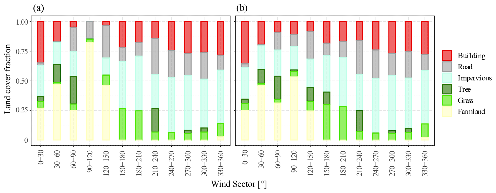
Figure B1 Land cover fraction for 30^∘ wind sectors but varying footprint length (Sect. 2.4) around the MY flux tower for (a) day ($K_{\downarrow }>\mathrm{5}$ W m⁻²) and (b) night.

The coefficients used (Table B1) include values obtained from 30 min measured data of net radiation (Q^*) and soil heat flux (Q_G) at the Weishan Experimental Station (36^∘39^′ N, 116^∘09^′ E). Weishan and MY have a similar climate background, the same wheat–maize rotation pattern, and a consistent growth cycle (Lei and Yang, 2010; Lei et al., 2018).

The Weishan station has a 10 m tower with a four-component radiometer (CNR1, Kipp & Zonen, the Netherlands) installed at 3.5 m a.g.l. and two soil heat flux plates (HFP01SC, Hukseflux, Netherlands) installed at a depth of −0.03 m. The instrument data are recorded at 10 min intervals using a CR10X data logger (Campbell Scientific, Inc., USA). The soil heat flux (Q_G) data are the average of two measurement sites to the east and west of the tower.

For application convenience, the cropland coefficients are determined by season. A random but an arbitrary 70 % of data are selected in each season to fit the coefficients. The remaining 30 % is used to evaluate the simulation results. The results are good but poorest in winter (Fig. B2). These values are used for the farmland (Table B1). Some large observed Q_G values are not reproduced by the OHM model, as they are the maximum values and appear simultaneously with the peak of Q^* on that day. Generally, the maximum Q_G appears later than that of Q^*, with the fitted a₂ of farmland being negative in all seasons (Table B1). This phenomenon has been reported in previous studies; i.e., OHM estimates perform satisfactorily in the mean but miss short-term variability (Grimmond and Oke, 1999b; Roberts et al., 2006).

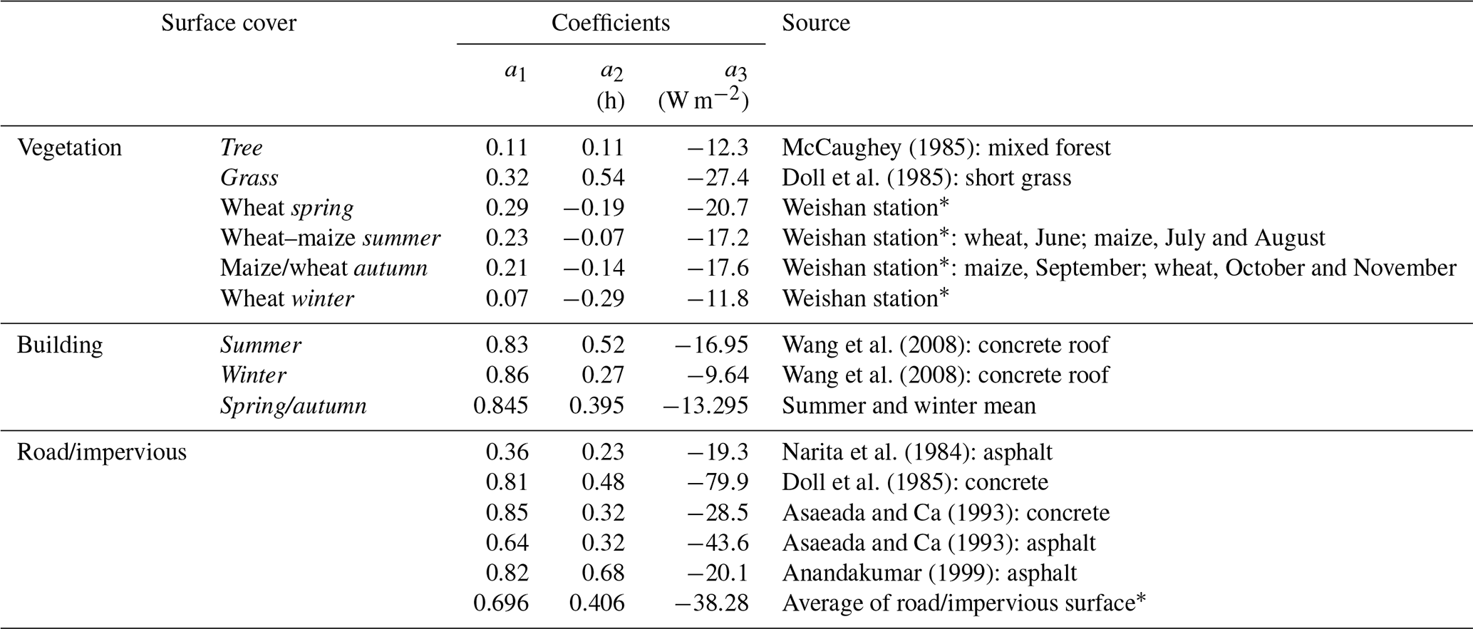
Building coefficients also vary with season (Table B1). Here we use data from Nanjing City (Wang et al., 2008), with an average of summer and winter values used in spring and autumn. Other coefficients are used year round. For the road/impervious areas, an average of the literature values is used (Table B1).

The MY site coefficients vary with season and time of day (Fig. B3). The a₁ and a₂ values are larger in the afternoon, as the wind comes from the southwest direction where artificial underlying surfaces dominate (Figs. 2g–j and B1). The a₁ and a₂ values of various impervious surfaces are relatively high (Table B1). The winter a₁ and a₂ values are smaller than other seasons throughout the day. This is because the prevailing wind in winter comes from the farmland-dominated direction, while the a₁ and a₂ values of farmland in winter are the smallest (Table B1). The a₃ value is exactly the opposite of a₁ and a₂.

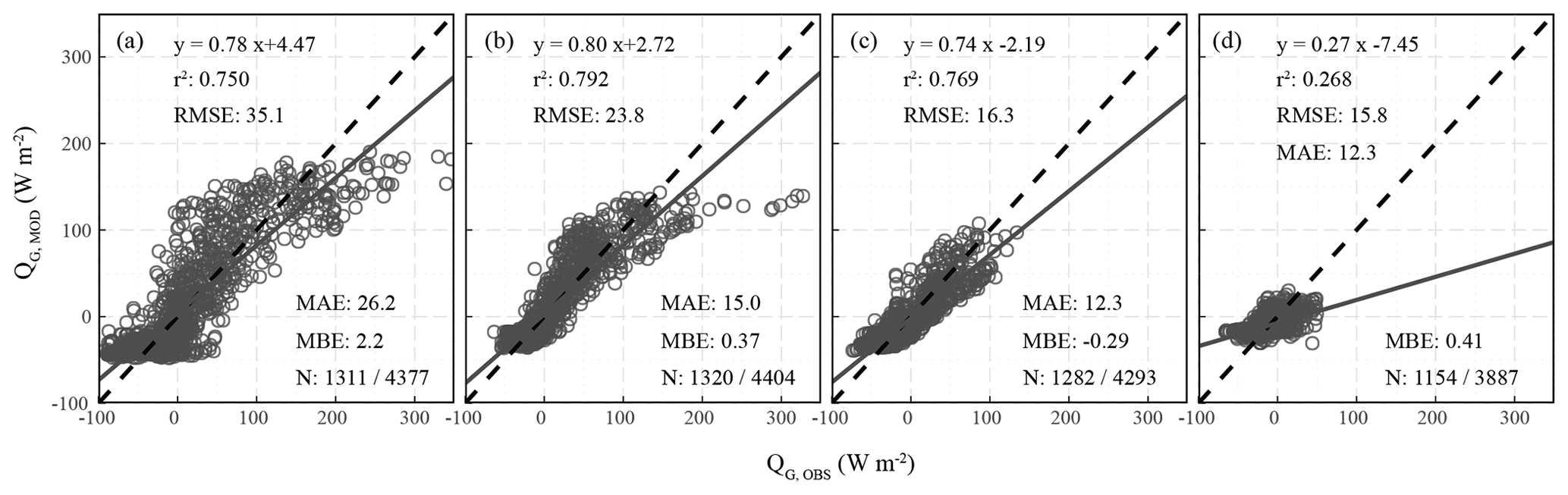
Figure B2 Weishan station modeled and observed soil heat flux, with statistical evaluation metrics: root mean square error (RMSE), coefficient of determination (r²), mean absolute error (MAE), and mean bias error (MBE). N: evaluation data/total observations available for (a) spring, (b) summer, (c) autumn, and (d) winter.

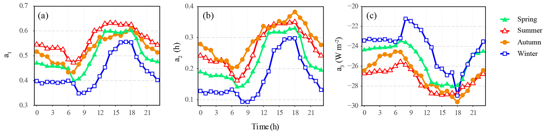
Figure B3 Seasonal diurnal variation in OHM coefficients (a) a₁, (b) a₂, and (c) a₃ for Miyun.

Table B1 Coefficients used for the OHM (Eq. B1) are from the literature or are derived in this study (^*).