Quantifying stratospheric ozone trends over 1984–2020: a comparison of ordinary and regularized multivariate regression models

Accurate quantification of long-term trends in stratospheric ozone can be challenging due to their sensitivity to natural variability, the quality of the observational datasets, and non-linear changes in forcing processes as well as the statistical methodologies. Multivariate linear regression (MLR) is the most commonly used tool for ozone trend analysis; however, the complex coupling in many atmospheric processes can make it prone to the issue of over-fitting when using the conventional ordinary-least-squares (OLS) approach. To overcome this issue, here we adopt a regularized (ridge) regression method to estimate ozone trends and quantify the influence of individual processes. We use the Stratospheric Water and OzOne Satellite Homogenized (SWOOSH) merged dataset (v2.7) to derive stratospheric ozone profile trends for the period 1984–2020. Besides SWOOSH, we also analyse a machine-learning-based satellite-corrected gap-free global stratospheric ozone profile dataset from a chemical transport model (ML-TOMCAT) and output from a chemical transport model (TOMCAT) simulation forced with European Centre for Medium-Range Weather Forecasts (ECMWF) ERA5 reanalysis.

For 1984–1997, we observe smaller negative trends in the SWOOSH stratospheric ozone profile using ridge regression compared to OLS. Except for the tropical lower stratosphere, the largest differences arise in the mid-latitude lowermost stratosphere (>4 % per decade difference at 100 hPa). From 1998 and the onset of ozone recovery in the upper stratosphere, the positive trends estimated using the ridge regression model (∼1 % per decade near 2 hPa) are smaller than those using OLS (∼2 % per decade). In the lower stratosphere, post-1998 negative trends with large uncertainties are observed and ridge-based trend estimates are somewhat smaller and less variable in magnitude compared to the OLS regression. Aside from the tropical lower stratosphere, the largest difference is around 2 % per decade at 100 hPa (with ∼3 % per decade uncertainties for individual trends) in northern mid-latitudes. For both time periods the SWOOSH data produce large negative trends in the tropical lower stratosphere with a correspondingly large difference between the two trend methods. In both cases the ridge method produces a smaller trend. The regression coefficients from both OLS and ridge models, which represent ozone variations associated with natural processes (e.g. the quasi-biennial oscillation, solar variability, El Niño–Southern Oscillation, Arctic Oscillation, Antarctic Oscillation, and Eliassen–Palm flux), highlight the dominance of dynamical processes in controlling lower-stratospheric ozone concentrations. Ridge regression generally yields smaller regression coefficients due to correlated explanatory variables, and care must be exercised when comparing fit coefficients and their statistical significance across different regression methods.

Comparing the ML-TOMCAT-based trend estimates with the ERA5-forced model simulation, we find ML-TOMCAT shows significant improvements with much better consistency with the SWOOSH dataset, despite the ML-TOMCAT training period overlapping with SWOOSH only for the Microwave Limb Sounder (MLS) measurement period. The largest inconsistencies with respect to SWOOSH-based trends post-1998 appear in the lower stratosphere where the ERA5-forced model simulation shows positive trends for both the tropics and the mid-latitudes. The large differences between satellite-based data and the ERA5-forced model simulation confirm significant uncertainties in ozone trend estimates, especially in the lower stratosphere, underscoring the need for caution when interpreting results obtained with different regression methods and datasets.

1 Introduction

With the success of the Montreal Protocol and its amendments, the emission of major ozone-depleting substances (ODSs) has greatly reduced and observations show decreases in their atmospheric concentrations (e.g. Anderson et al., 2000; Solomon et al., 2006; Chipperfield et al., 2017; Montzka et al., 2021). However, quasi-global total column ozone does not show a statistically significant ozone increase (WMO, 2022, and references therein). To a certain extent, there is a scientific consensus that the ODS-related positive ozone trends are balanced by the negative contributions from atmospheric dynamics (e.g. Weber et al., 2022; Bognar et al., 2022). As the impacts of chemical and dynamical processes on ozone variability are variable across the stratosphere, accurate quantification of stratospheric ozone trends remains an unresolved challenge.

An important aspect of long-term ozone trends that has been confirmed by various recent studies is that there is an ozone increase in the upper stratosphere (e.g. Harris et al., 2015; Chipperfield et al., 2017; Sofieva et al., 2017; Ball et al., 2017; Steinbrecht et al., 2017; Petropavlovskikh et al., 2019; Godin-Beekmann et al., 2022), partly due to the decreased ODS concentrations and partly due to the stratospheric cooling resulting from increased greenhouse gases (GHGs). However, our understanding about the evolution of lower-stratospheric ozone remains highly uncertain. Various observation-based studies suggest that there has been a continued decline in lower-stratospheric ozone since 1998, in both the tropics and the mid-latitudes (e.g. Ball et al., 2018, 2019a; Wargan et al., 2018; Orbe et al., 2020; Bognar et al., 2022), while model simulations do not reproduce these trends (Ball et al., 2020; Dietmüller et al., 2021; Davis et al., 2023; Li et al., 2022a). It is well established that ozone in the lower stratosphere is sufficiently long-lived and primarily controlled by transport and circulation changes (e.g. Chipperfield et al., 2018). The increasing GHGs induce a strengthening of tropical upwelling and enhance the stratospheric circulation, which causes tropical ozone to decline in the lower stratosphere (Marsh et al., 2016). Besides, the non-linear quasi-biennial oscillation (QBO) and the El Niño–Southern Oscillation (ENSO) influence the dynamical variability in the lower stratosphere and drive the large interannual ozone variability in this region (Ball et al., 2019a; Diallo et al., 2018). The asymmetrical change pattern in the Brewer–Dobson circulation (BDC), with a relative slowdown in the Northern Hemisphere (NH), also provides evidence pointing to dynamically driven ozone variability in the lower stratosphere (e.g. Mahieu et al., 2014; Stiller et al., 2017; Prignon et al., 2021; Bognar et al., 2022). Considering the inconsistencies between observations and model simulations, it is important to gain better insight about the causes of uncertainties in the estimates of the lower-stratospheric ozone trends.

Most importantly, not only is the quantification of stratospheric ozone trends sensitive to natural variability and non-linear forcing processes, but also it depends on the quality of the observational datasets and the time periods considered. To determine the long-term ozone trends and the attribution of ozone variability, composites of observations are generally used by merging different ozone observational datasets into a long, multi-decadal record. However, there are artefacts in the uncertainty budget and sampling inconsistencies between various datasets. Previous studies have used multiple composites merged from different observing platforms and discussed the sensitivity of ozone trends to the inclusion of new datasets (Ball et al., 2018, 2019a; Sofieva et al., 2017, 2023; Steinbrecht et al., 2017; Petropavlovskikh et al., 2019; Weber et al., 2022; Godin-Beekmann et al., 2022). Here, we use the merged Stratospheric Water and OzOne Satellite Homogenized (SWOOSH, version 2.7) dataset to assess the stratospheric ozone trends (Davis et al., 2016) for the 1984–2020 time period. In addition, a machine-learning-based satellite-corrected gap-free global stratospheric ozone profile dataset from a chemical transport model (ML-TOMCAT; Dhomse et al., 2021a) is also used for comparison.

To improve the assessment of the long-term ozone trends and variability, multivariate linear regression (MLR) models with different configurations are most widely used by separating the influence of various chemical and dynamical processes on the ozone concentrations (e.g. Dhomse et al., 2006, 2022; Chehade et al., 2014; Li et al., 2020, 2022a). Szeląg et al. (2020) analysed the seasonal dependence of stratospheric ozone trends from four merged satellite datasets over 2000–2018 using a two-step MLR approach. Godin-Beekmann et al. (2022) presented the evaluation of stratospheric ozone profile trends in the extra-polar region over the period 2000–2020 with an updated version of the Long-term Ozone Trends and Uncertainties in the Stratosphere (LOTUS) regression model which additionally included seasonal trend terms. Bognar et al. (2022) used both MLR and dynamical linear modelling (DLM) methods (Laine et al., 2014; Ball et al., 2017, 2019a) to determine the stratospheric ozone trends during 2000–2021 with a combination of three satellite datasets. Recently, Dhomse et al. (2022) used an ensemble of MLR models and regularized regression methods (ridge, lasso, and elastic net) to estimate the solar cycle signal in the observed and simulated ozone profiles for 2005–2020. With the extended datasets and improved statistical methodologies, there is better agreement about and reduced uncertainties in different satellite-based ozone trends. However, it should be noted that trends in the lower stratosphere are still masked by large dynamical/natural variability.

Additional complications also arise from the use of chemical/dynamical proxies in the MLR; some of them are inevitably correlated and coupled, causing an issue of over-fitting (e.g. Dhomse et al., 2022), which will significantly lead to inconsistent and unreliable parameter estimates in regression modelling (e.g. Shariff and Duzan, 2018). To overcome this over-fitting problem, regularized regression models such as ridge regression are highly recommended (e.g. Hoerl and Kennard, 1970). Previous studies have indicated that ridge regression performs better than other estimators and can produce reliable results when explanatory variables are correlated (e.g. Shariff and Duzan, 2018; Tirink et al., 2020; Gana, 2022). In this paper, we use MLR models based on both ordinary-least-squares (OLS) and ridge regression methods to compare and discuss their differences in estimating stratospheric ozone trends. Besides SWOOSH and ML-TOMCAT datasets, a chemical transport model (TOMCAT) simulation forced with the European Centre for Medium-Range Weather Forecasts (ECMWF) ERA5 reanalyses (Li et al., 2022a) is also used for comparison with satellite-based ozone trends and ozone changes associated with natural variability.

The paper is organized as follows. Section 2 describes the merged satellite-based ozone dataset (SWOOSH), a TOMCAT model simulation forced with ECMWF ERA5 reanalyses (hereafter ERA5), and a machine-learning-based satellite-corrected TOMCAT product (ML-TOMCAT). Section 3 describes the MLR models and regression methods based on OLS and ridge. Section 4 presents results regarding the ozone profile trends based on OLS and ridge regression methods and the ozone variations associated with natural processes. Our conclusions are summarized in Sect. 5.

2 Data

2.1 SWOOSH

The Stratospheric Water and OzOne Satellite Homogenized (SWOOSH) dataset is a monthly mean record of stratospheric ozone and water vapour data from a subset of limb sounding and solar occultation satellites operating from 1984 to the present (Davis et al., 2016). It is obtained from https://csl.noaa.gov/groups/csl8/swoosh/ (last access: 10 January 2023). The SWOOSH (v2.7) record is comprised of several individual satellite data from the Stratospheric Aerosol and Gas Experiment (SAGE-II/SAGE-III v7/v4), the Upper Atmospheric Research Satellite Halogen Occultation Experiment (UARS HALOE v19), the UARS Microwave Limb Sounder (MLS v5/6), the Aura MLS (v5), the Aura High Resolution Dynamics Limb Sounder (HIRDLS v7) and the Atmospheric Chemistry Experiment Fourier Transform Spectrometer (ACE-FTS v3.6) instruments, as well as a combined data product. The corrections that vary with latitude and height are determined from coincident observations closely matched in space and time during time periods of instrument overlap. The primary SWOOSH product consists of zonal-mean values at grids of 2.5, 5, and 10^∘ resolution. There are filled and unfilled versions of the dataset at both geographical and equivalent-latitude coordinates. Many previous studies have demonstrated the reliability of this product in analysing the variability and mechanisms associated with stratospheric ozone (e.g. Lu et al., 2019; Shangguan et al., 2019; Zhang et al., 2021; Hu et al., 2022). Here we use the gap-filled SWOOSH data at grids of 2.5^∘ and 12 levels per decade ranging from 316 to 1 hPa (31 pressure levels). These SWOOSH data are considered a beta product and will continue to be updated as long as new data are available from the Aura MLS instrument or a suitable replacement.

2.2 TOMCAT simulation

Chemical transport models (CTMs) are important tools for understanding past ozone changes by combining up-to-date knowledge about various physical and chemical processes within a mathematically consistent framework. TOMCAT/SLIMCAT (hereafter TOMCAT) is a global 3-D off-line CTM (Chipperfield, 2006), which contains a detailed description of stratospheric chemistry (e.g. Feng et al., 2011, 2021; Dhomse et al., 2015, 2016; Chipperfield et al., 2018) or tropospheric chemistry (Monks et al., 2017) and uses winds and temperatures from meteorological analyses (usually ECMWF) to specify the atmospheric transport and temperatures.

Here we have performed a TOMCAT simulation (ERA5), which is forced with ECMWF ERA5 (Hersbach et al., 2020) reanalysis (e.g. Dhomse et al., 2019; Feng et al., 2021; Li et al., 2022a). The ERA5 reanalysis has been released by ECMWF to supersede ERA-Interim, which covered January 1979 to August 2019, with more and newer observations assimilated into ERA5. The inhomogeneities in reanalysis datasets could introduce spurious transport features (e.g. Schoeberl et al., 2003; Ploeger et al., 2015) and thus cause an inability of chemical models to simulate the observed stratospheric ozone changes (Li et al., 2022a). The TOMCAT simulation is identical to that used in Li et al. (2022a), with $\mathrm{2.8}{}^{\circ }\times \mathrm{2.8}{}^{\circ }$ (T42 Gaussian grid) horizontal resolution and 32 hybrid sigma–pressure levels ranging from the surface to about 60 km. The 6-hourly grid point meteorological fields are interpolated linearly in time for the simulation.

2.3 ML-TOMCAT

We use a machine-learning-based method and chemically self-consistent output from the TOMCAT 3-D CTM to create a satellite-corrected long-term stratospheric ozone profile dataset (ML-TOMCAT, Dhomse et al., 2021a). The TOMCAT setup is described in Sect. 2.2 above. A random-forest (RF) regression model, including five terms: passive ozone (O₃), HCl mixing ratio (HCl), methane mixing ratio (CH₄), Mg II solar flux term (MgII), and observation–model total column ozone difference (dTCO) is applied to the observation–model ozone difference by selecting 20 years of UARS MLS (1991–1998) and Aura MLS (2005–2016) measurements as a training period. The passive O₃, HCl, and CH₄ are tracers taken from TOMCAT output fields; dTCO is calculated from Copernicus Climate Change Service (C3S) total ozone data; and the MgII index (Snow et al., 2014) is obtained from http://www.iup.uni-bremen.de/UVSAT/ Datasets/mgii (last access: 10 January 2023). These variables account for possible biases in CTM profiles due to transport, solar flux variability, or the use of coarse spectral bins (e.g. Dhomse et al., 2013; Sukhodolov et al., 2016; Feng et al., 2021).

The results show that ML-TOMCAT ozone concentrations are in excellent agreement with SWOOSH data and that they are well within uncertainties of the observational datasets at almost all stratospheric levels. ML-TOMCAT is also ideally suited for the evaluation of chemical model ozone profiles and observation-based datasets from the tropopause up to 0.1 hPa. The ML-TOMCAT ozone profile data (v1.0) on pressure and altitude levels in mixing ratios and number density units are available via https://doi.org/10.5281/zenodo.5651194 (Dhomse et al., 2021b).

3 Methods

3.1 Multivariate linear regression models

Here we use multivariate linear regression (MLR) models to estimate the stratospheric ozone trends and to separate the influence of important chemical and dynamical processes on the ozone variations. The MLR setup is a modified version of that used in Dhomse et al. (2022). Briefly, it has 77 terms, including 24 monthly linear trend terms and 24 intercept terms for the independent linear trends (ILTs; e.g. Weber et al., 2018) before and after the turnaround year (1997) close to the timing of the peak stratospheric halogen loading; 24 QBO terms at 30 and 50 hPa; and 5 proxies for the 11-year solar cycle, El-Niño–Southern Oscillation (ENSO), Arctic Oscillation (AO), Antarctic Oscillation (AAO), and Eliassen–Palm (EP) flux. QBO, ENSO, AO, and AAO indices are from the Climate Prediction Center (https://www.cpc.ncep.noaa.gov/, last access: 10 January 2023). The proxy for EP flux uses the 50 hPa vertical component ($F_{z_{\mathrm{50}}}$) with 2-month mean values (averaged over previous and current months) integrated over mid-latitudes between 45 and 75^∘ in each hemisphere from the ECMWF ERA5 reanalysis. The effects of the aerosol loading from volcanic eruptions (e.g. Mt Pinatubo, 1991) are not considered in the MLR as we remove the data from 1991 to 1994. Here, we use 12 (monthly) trend terms instead of 1 (annual) as it is better at capturing seasonal patterns and has better sensitivity to short-term fluctuations and improved flexibility that means better goodness of fit (R²). Also, more proxies are considered to account for the dynamical variability in stratospheric ozone and to separate the influence of individual processes (e.g. Dhomse et al., 2022; Weber et al., 2022).

We apply the MLR to monthly mean ozone anomalies and get

$$\mathrm{d}{\mathrm{O}}_{\mathrm{3}}\left(t\right)=\sum _{j=\mathrm{1}}^{\mathrm{77}}{\mathit{\beta }}_j\times P_j\left(t\right)+\mathit{ϵ}\left(t\right),$$

where dO₃(t) denotes monthly mean ozone anomaly time series from 1984–2020 obtained by referencing the monthly mean O₃(t) to the climatological mean for each calendar month. The explanatory proxies P_j include 77 terms which are de-trended (except for the linear trend terms) and normalized between 0 and 1. The coefficients β_j are obtained by least-squares fitting of the residuals. By de-trending, the long-term trends in various proxies are moved to the linear trend terms; that is, the independent linear trends in the MLR combine both the dynamic and the ODS-related chemical trends (Weber et al., 2022).

As noted earlier, as most atmospheric processes are not completely independent, the MLR models suffer from over-fitting issues to a certain extent. Here we use both ordinary-least-squares (OLS) and regularized (ridge) linear regression models for comparison to quantify the estimated ozone trends and the influence of individual processes.

3.2 OLS regression

Ordinary-least-squares (OLS) regression is a common method used to study the relationship between explanatory variables and response variables in regression models. The OLS method aims to minimize the sum of squared errors (SSE) between the observed values (y_i) and predicted values ($\widehat{y_i}$). The cost function being minimized is written as

$$\text{minimize}\left(\text{SSE}=\sum _{i=\mathrm{1}}^n(y_i-\widehat{y_i}{)}^{\mathrm{2}}\right).$$

It should be noted that the OLS with unbiased estimators performs well only when all key regression assumptions are satisfied, e.g. a linear relationship, more observations (n) than features (p), and no or little collinearity among the explanatory variables. Additionally, the OLS model is designed to minimize the residual errors but with relatively high variance, which means small changes in explanatory variables can lead to large changes in the estimated regression coefficients. Thus, care is needed when analysing the results of parameter estimates and inference under the OLS procedure.

3.3 Ridge regression

To overcome the over-fitting issue in regression, several methods have been developed, and the most common is ridge regression (Hoerl and Kennard, 1970). Ridge regression is a type of regularized regression which adds a penalty (called an L2 penalty) as described in Hastie et al. (2009) and Kuhn and Johnson (2013) to constrain the magnitudes and fluctuations of the coefficient estimates. This constraint helps to reduce the variance of the model at the expense of no longer being unbiased, which is a reasonable compromise. The cost function with a penalty term is written as

$$\text{minimize}\left(\text{SSE}+\mathit{\alpha }\sum _{j=\mathrm{1}}^p{\mathit{\beta }}_j^{\mathrm{2}}\right).$$

The penalty is calculated as the square of the magnitude of coefficients. By adding this penalty term, all coefficients of the regression variables (β_j) will be constrained or shrunk, but not to zero, so they all remain in the model. The strength of the penalty term is controlled by a tuning parameter (α). When this tuning parameter is set to zero, ridge regression equals OLS regression. If α=∞, all coefficients in the regression are shrunk to zero. The ideal penalty is therefore somewhere in between 0 and ∞, which helps to control the model in terms of over-fitting or under-fitting. Here we use cross-validation (CV) to identify the optimal α value (Pedregosa et al., 2011). The ridge regression model used here is from the Python scikit module (for details see https://scikit-learn.org/stable/modules/linear_model.html, last access: 10 January 2023).

Figure 1 shows the SWOOSH ozone anomalies and fitting from OLS and ridge regression models near the Equator (∼1^∘ N) at pressure levels of 1, 10, and 46.4 hPa. The cross-validated mean square error (MSE), that is, the average of all the test MSEs calculated from different training and testing sets, and coefficients for the ridge regression model are also shown as the α value grows from 0.01 to 100. In all cases shown in Fig. 1, we find a slight improvement in the MSE as the penalty (α) gets larger, suggesting that a regular OLS model likely over-fits the training data. As the penalty continues to increase, coefficients in the ridge regression model are shrunk until close to zero. The vertical dashed lines represent the optimal α value with the minimum MSE (α₀= 0.174, 0.048, and 0.026 in ridge regression for ozone anomaly data at pressure levels of 1, 10, and 46.4 hPa). Monthly mean ozone anomalies as well as the OLS and ridge fitting from ML-TOMCAT and simulation ERA5 are shown in the Supplement (Figs. S1–S2).

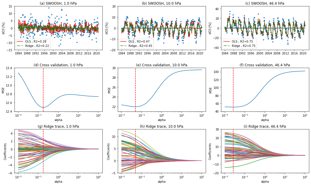
Figure 1 (a–c) Monthly mean ozone anomalies (blue dots) and the OLS (red line) and ridge fitting (dash-dotted green line) from SWOOSH data during 1984–2020 at the pressure levels of 1 hPa (a, d, g), 10 hPa (b, e, h), and 46.4 hPa (c, f, i) for the 1^∘ N latitude. (d–f) Cross-validated MSE values as well as (g–i) the ridge regression trace of the coefficients that change with alpha (α) are also shown. The vertical dashed red line indicates the optimal tuning value (α₀) for ridge regression where MSE is minimum.

As expected, goodness-of-fit (R²) values for ridge regression are smaller than OLS whenever the ozone data are noisy and the regression model is not able to attribute ozone variations to any explanatory variables (e.g. upper stratosphere). However, R² differences are smaller when one or multiple variables are able to explain ozone variations (e.g. lower stratosphere). We use the Cochrane–Orcutt method to correct for the first-order autocorrelation (AR1) in the residuals of an OLS regression model. The procedure is performed iteratively with the covariance matrix updated for each iteration until the autocorrelation coefficient has converged sufficiently (Cochrane and Orcutt, 1949; Prais and Winsten, 1954). This correction for AR1 in the OLS regression model is widely used for the trends from monthly mean ozone time series (e.g. Dhomse et al., 2006; Ball et al., 2019a; Petropavlovskikh et al., 2019; Bognar et al., 2022; Godin-Beekmann et al., 2022). However, ridge regression, which constrains the fit coefficients by introducing a penalty term, is different from the linear unbiased estimates of the usual least-squares method. If we still apply the AR1 correction to ridge regression similarly to OLS regression, the estimated regression coefficients can be affected; the correlation between the regression model and underlying data becomes very poor after “correction”, and the regression in this case is under an “under-fitting” state with a very large tuning parameter. Besides, the autocorrelation coefficient does not always converge during iteration, which makes it impossible to obtain the covariance matrix as in OLS regression. Given all this, we do not apply the AR1 correction to ridge regression here, and care must be taken regarding the limitations and assumptions of the Cochrane–Orcutt method.

4 Results and discussion

4.1 Ozone profile trends with OLS and ridge regression

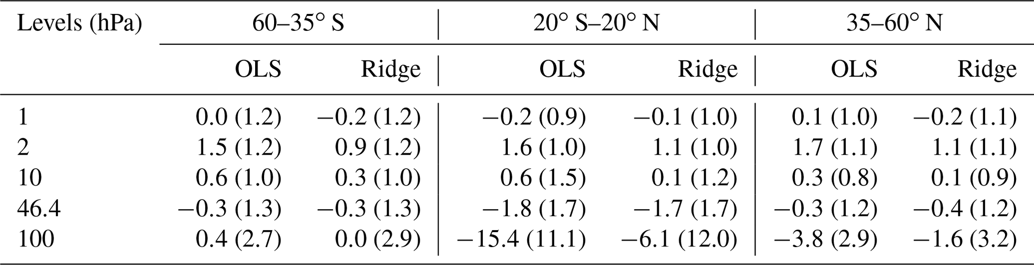
Figure 2 shows the annual mean stratospheric ozone profile trends (percent per decade) comparing between OLS and ridge regression methods for three latitude bands (60–35^∘ S, 20^∘ S–20^∘ N, and 35–60^∘ N) from SWOOSH, ML-TOMCAT, and the model simulation ERA5 over the period 1984–1997. The trend results as well as the 2σ uncertainties (the standard deviation of the trends) for several pressure levels (1, 2, 10, 46.4, and 100 hPa) are given in Table 1. The annual mean trend is the average of the 12-monthly means, and the uncertainty in the annual trend is the standard deviation from taking the mean from the monthly values.

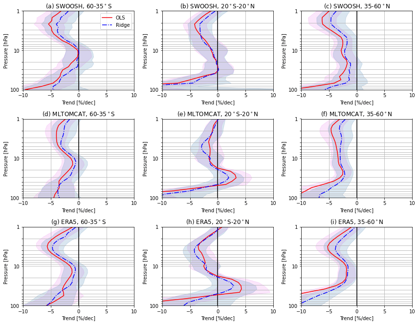
Figure 2 Profiles of annual mean stratospheric ozone trends (percent per decade) derived from OLS and ridge regression methods for three latitude bands (60–35^∘ S, 20^∘ S–20^∘ N, and 35–60^∘ N) from (a–c) SWOOSH, (d–f) ML-TOMCAT, and (g–i) model simulation ERA5 over the period 1984–1997. Shaded regions indicate 2σ uncertainties.

Table 1 Stratospheric ozone trends with 2σ uncertainties (in percent per decade) from SWOOSH during 1984–1997 based on OLS and ridge regression.

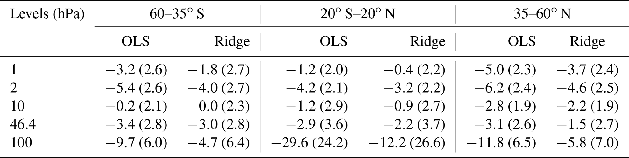
With ridge regression, the stratospheric ozone profile trends from SWOOSH data show smaller declines during 1984–1997 compared to OLS-based trend estimates. As shown in Fig. 2a–c and Table 1, large OLS–ridge differences appear in the upper stratosphere (∼1 % per decade at 2 hPa) and the lowermost stratosphere (>4 % per decade at 100 hPa). Compared with the trend profiles derived from OLS regression, the ridge regression model has less variability and smaller absolute fit coefficients (especially at mid-latitudes). These differences in trend values are likely due to the fundamental differences between the two regression methods. The largest ozone decreases appear in the tropical lower stratosphere (with about −30 % per decade for OLS and −12 % per decade for ridge regression) although there are large uncertainties (>20 % per decade). These large uncertainties to some extent are associated with the considerable dynamical variability near the tropopause (e.g. Sofieva et al., 2014; Thompson et al., 2021; Bognar et al., 2022) and are also related to the quality of the satellite data and limitations in sampling and resolution (Davis et al., 2016). The negative ozone trend estimates from ML-TOMCAT and simulation ERA5 show very good agreement with those from SWOOSH data at mid-latitudes in both the Northern Hemisphere (NH) and the Southern Hemisphere (SH). Large differences appear in the tropical middle and lower stratosphere where ML-TOMCAT and the ERA5-forced model simulation show positive trends with a range of 2 %–4 % per decade near 30 hPa, but SWOOSH data show a near-zero trend. We note that there are large uncertainties in the lower stratosphere for both satellite data and model simulations.

As shown in Fig. 3, upper-stratospheric ozone has increased since 1998 across all three latitude bands and the increases based on ridge regression are slightly smaller. Table 2 gives some trend results and corresponding 2σ uncertainties from SWOOSH data during 1998–2020. The significant positive ozone trends (∼2 % per decade for OLS regression) in the upper stratosphere are consistent with the statistically significant trends shown in previous studies (Ball et al., 2017; Sofieva et al., 2017; Steinbrecht et al., 2017; Bourassa et al., 2018; WMO, 2018; Petropavlovskikh et al., 2019; Godin-Beekmann et al., 2022; Bognar et al., 2022). The largest increase based on ridge regression is 1.1±1.1 % per decade near 2 hPa at NH mid-latitudes, 1.1±1.0 % per decade near 2 hPa in the tropics, and 1.3±0.8 % per decade at 3.8 hPa at SH mid-latitudes. In the middle and lower stratosphere, ozone trends are generally negative except for the non-significant positive trends near 20 hPa at SH mid-latitudes, where a large difference of ∼1.3 % per decade occurs between OLS and ridge regression methods. Negative trends with larger uncertainties are observed in the lower stratosphere, which are most pronounced in the tropics ($-\mathrm{6.1}\pm \mathrm{12.0}$ % per decade at 100 hPa), followed by the decrease at NH mid-latitudes ($-\mathrm{1.6}\pm \mathrm{3.2}$ % per decade at 100 hPa). The largest difference between OLS and ridge regression methods occurs in the tropical lowermost stratosphere with a difference of ∼9 % per decade at 100 hPa (but with larger uncertainties >10 % per decade for both regression methods), followed by the NH mid-latitudes with >2 % per decade difference at 100 hPa (∼3 % per decade uncertainties). Note that, despite the large differences between OLS- and ridge-based trends, they are still within the uncertainties of the individual trends. The observed ozone decreases in the lower stratosphere are similar to recent records (e.g. Ball et al., 2019a; 2020; Godin-Beekmann et al., 2022), which could be explained by the increased tropical upwelling and mid-latitude mixing (Wargan et al., 2018; Ball et al., 2020; Orbe et al., 2020; Davis et al., 2023). Nevertheless, the modelled lower-stratospheric trends do not match those derived from observations.

Figure 3 Same as Fig. 2 but for the post-1998 time period (1998–2020).

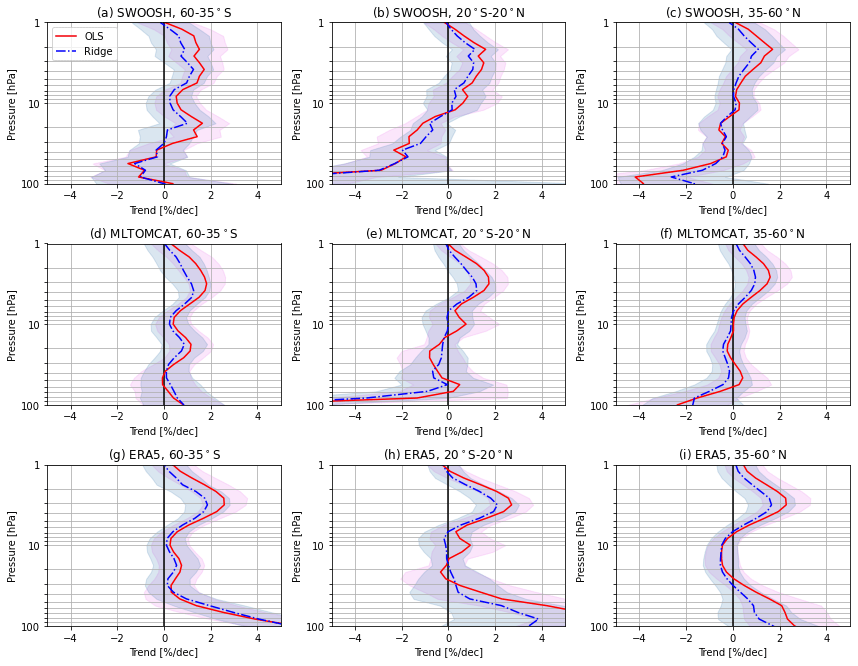
Table 2 Stratospheric ozone trends with 2σ uncertainties (in percent per decade) from SWOOSH during 1998–2020 based on OLS and ridge regression.

Compared to the trend estimates from simulation ERA5 in Fig. 3, the ML-TOMCAT dataset shows more consistent results with the SWOOSH data, with negative ozone trends in the tropical and NH mid-latitude lower stratosphere. The better agreement between ML-TOMCAT and SWOOSH, due to satellite corrections derived from the same MLS measurements, shows some improvements in this machine-learning-based dataset compared to the TOMCAT CTM. The largest differences between SWOOSH-based and ML-TOMCAT-based ozone trends appear in the SH mid-latitude lower stratosphere, where ML-TOMCAT shows positive trends, and in the tropical middle and lower stratosphere with close-to-zero trends near 60 hPa (although these trends have large uncertainties). On the other hand, trends from model simulation ERA5 show the largest inconsistencies with respect to SWOOSH-based trends in the lower stratosphere. Simulation ERA5 shows positive trends for all three latitude bands, but these trends are more pronounced in the SH mid-latitudes (5.4±2.0 % per decade at 100 hPa for ridge regression). These differences between satellite-based datasets and model simulation suggest there are still large uncertainties in the lower stratosphere where dynamical processes dominate (Dietmüller et al., 2021; Li et al., 2022a). Ball et al. (2020) reported significant discrepancies in observation–model lower-stratospheric ozone trends by using various satellite-based datasets and chemistry–climate models (CCMs). Although the inconsistencies vary with various datasets and fit methods (Dietmüller et al., 2021; Bognar et al., 2022), models generally do not reproduce the observations, and the reason for this remains an open question.

Similarly to SWOOSH-derived trends, the ridge-based trends from ML-TOMCAT and simulation ERA5 are smaller in magnitude when compared to OLS-based trends. An evident OLS–ridge difference appears at near 10 hPa in the tropical stratosphere, where OLS-based trends from both ML-TOMCAT and simulation ERA5 show a small peak (∼1 % per decade) but ridge-based trends are close to zero. This difference between OLS and ridge regression might be associated with the regression methods and correction used for the autoregression (AR1). Although the AR1 correction is applied to OLS regression, we should be aware of the limitations of the Cochrane–Orcutt method; i.e. it is specifically designed to handle first-order autocorrelation (AR1). If the autocorrelation in the residuals follows a higher-order AR process or a different pattern, this method may not be appropriate or effective. Besides, the estimated regression coefficients and their interpretation can be affected for the corrected model with the application of the Cochrane–Orcutt method.

The seasonal variations in stratospheric ozone trends from SWOOSH data during 1998–2020 are averaged over three latitude bands (60–35^∘ S, 20^∘ S–20^∘ N, 35–60^∘ N) and compared using both OLS and ridge regression methods, as shown in Fig. 4. There is a strong seasonal dependence in stratospheric ozone trends, with the signs of positive and negative trends varying with season and altitude. OLS-based trend estimates are in good agreement with those in previous studies (e.g. Szeląg et al., 2020). Positive trends are observed in the upper stratosphere (10–1 hPa) for almost all seasons, with the maximum (>2 % per decade) in local winter at mid-latitudes, while in the tropics (near 1–3 hPa) negative trends of more than −1 % per decade appear in December–January–February (DJF). In the middle stratosphere (32–10 hPa), there is a hemispheric asymmetric structure with positive trends (1 % per decade–2 % per decade) in the SH mid-latitudes and negative trends (−1 % per decade) in the NH mid-latitudes in June–July–August (JJA). In the lower stratosphere (100–32 hPa), there are persistent negative trends for all seasons in the tropics, with the largest negative trends in May (< −4 % per decade) and negligible trends in March and April near 60 hPa. Trends in the NH mid-latitudes are more negative in the lowermost stratosphere compared to those in the SH mid-latitudes. In the SH mid-latitudes, there exists a clear transition from negative trends in February–July to positive trends in August–October. The ridge regression method shows very similar results to those using OLS except that the absolute ridge-based trends and fit coefficients are smaller.

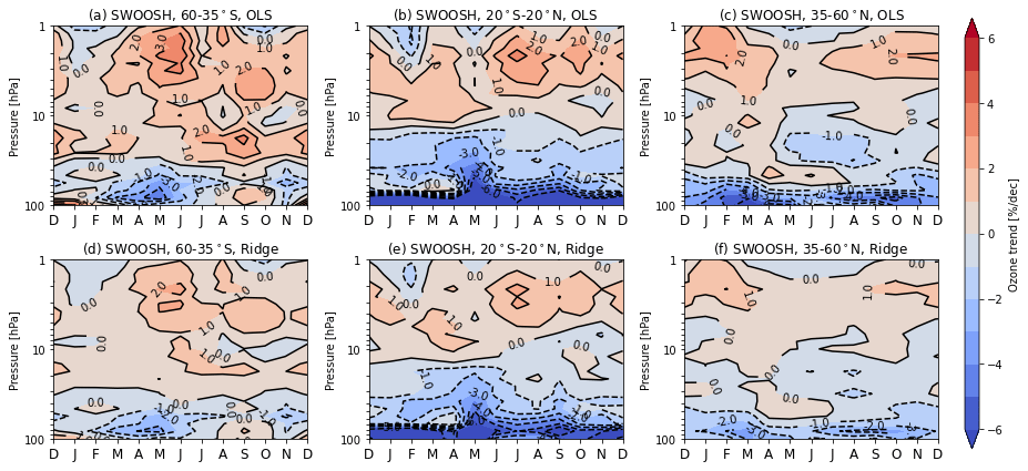
Figure 4 Pressure–season variation in linear trends in ozone (percent per decade) from SWOOSH data over 1998–2020 for three selected latitudinal bands (60–35^∘ S, 20^∘ S–20^∘ N, 35–60^∘ N) based on (a–c) OLS and (d–f) ridge regression methods.

Figure 5 shows the comparison of seasonal variations in stratospheric ozone trends over the post-1998 period from ML-TOMCAT data and model simulation ERA5 based on the ridge regression. Trends from ML-TOMCAT data show more consistency with those from SWOOSH data in seasonal dependence, while model-based estimates show significant differences. In the SH lowermost stratosphere, simulation ERA5 shows positive trends for all seasons, which is different from the trend pattern with seasonal dependence from SWOOSH and ML-TOMCAT data. In the tropical middle and lower stratosphere, there are large differences in seasonal ozone trends between model simulation and satellite data. Trends from simulation ERA5 show more positive trends for all seasons in the tropical lower stratosphere, which is opposite to the negative trends from SWOOSH and ML-TOMCAT. Also, simulation ERA5 shows more significant positive trends in the tropical lowermost stratosphere during winter and spring compared to ML-TOMCAT. In the NH lower stratosphere, the negative trends from ML-TOMCAT show better agreement with those from SWOOSH, while simulation ERA5 still shows opposite and weak positive trends in most months. The reason for the better agreement between ML-TOMCAT and SWOOSH-based trend estimates may be from the fact that denser MLS measurements that are part of SWOOSH are also used for the training of ML-TOMCAT model. These seasonal trends provide more information beyond the annual mean trends, which is helpful in further understanding the role of dynamical variability in short-term trends as well as the prediction of ozone recovery.

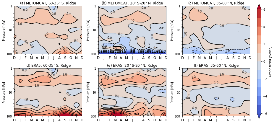
Figure 5 Pressure–season variation in linear trends in ozone (percent per decade) from (a–c) ML-TOMCAT and (d–f) simulation ERA5 over 1998–2020 for three selected latitudinal bands (60–35^∘ S, 20^∘ S–20^∘ N, 35–60^∘ N) based on the ridge regression method.

The post-1998 seasonal ozone profile trends averaged over the three latitude bands (60–35^∘ S, 20^∘ S–20^∘ N, 35–60^∘ N) from SWOOSH, ML-TOMCAT, and simulation ERA5 are presented and compared in Fig. S3 with ridge regression. The differences in the seasonal ozone profile trends using OLS and ridge regression methods are also shown in Fig. S4. Consistent with the monthly mean trend variations shown in Figs. 4–5, the ozone profile trends during post-1998 time periods show seasonal and altitude dependence for all datasets. The ML-TOMCAT dataset shows similar seasonal trends to those using SWOOSH data, while model simulation ERA5 shows larger inconsistencies especially in the lower stratosphere. The considerable differences suggest that there is a large degree of uncertainty in the estimates of seasonal ozone trends, particularly in the lower stratosphere, where dynamical processes dominate; in addition there is larger uncertainties in the satellite data. Therefore, caution is needed when discussing the results for this region, as neither regression method can reliably capture the large variability.

As shown in Fig. S4, the positive trends at SH mid-latitudes in the middle stratosphere (near 20–30 hPa) from SWOOSH data are constrained by ∼2 % per decade in September–October–November (SON) with ridge regression. Meanwhile, the negative trends in the NH mid-latitudes in JJA are also constrained by ∼0.7 % per decade compared to OLS regression. In the tropical lowermost stratosphere (near 100 hPa), the observed negative trends are constrained with ridge regression by more than 2 % per decade for all seasons. For ML-TOMCAT and simulation ERA5, trends in the tropical lower stratosphere also show large differences with a wide variability for different seasons. Despite these differences between OLS- and ridge-based ozone profile trends, the even larger uncertainties, e.g. in the lower stratosphere (Fig. S3), suggest the ozone trends from the two regression models are not different from each other.

4.2 Ozone variations associated with natural processes

The QBO at 30 and that at 50 hPa are important proxies used in the regression model to represent the variability in stratospheric ozone in the tropics as well as at higher latitudes (Anstey and Shepherd, 2014; Lu et al., 2019; Xie et al., 2020; Zhang et al., 2021; Wang et al., 2022). Figures 6–7 show the seasonal responses of stratospheric ozone to QBO at 30 and 50 hPa from SWOOSH, ML-TOMCAT, and simulation ERA5 over the long period 1984–2020 based on ridge regression. Similar results based on OLS regression are also presented in Figs. S5–S6. It is obvious that the seasonal cycle modulates the QBO at higher latitudes with more significant responses during local winter–spring (Tung and Yang, 1994; Wang et al., 2022). A double-peaked vertical structure of stratospheric ozone anomalies associated with QBO is also clear in the tropics for all seasons. All datasets show very consistent influences of QBO on ozone; however, there exist large seasonal QBO pattern differences between various datasets. In the mid-latitude lower stratosphere, model simulation ERA5 shows more negative ozone anomalies from the two QBO phases in all seasons compared to SWOOSH and ML-TOMCAT. In the tropics, there are more positive ozone responses to QBO in simulation ERA5 at near 30 hPa for all seasons (Fig. 6h) as well as below 50 hPa in DJF (Fig. 7h) when compared to ML-TOMCAT. The positive QBO influences on the tropical ozone and negative influences on the subtropical region are associated with the QBO phase changing from the Equator to the subtropics, which is consistent with previous studies of QBO signals in total column ozone (Tung and Yang, 1994; Chehade et al., 2014; Li et al., 2022a).

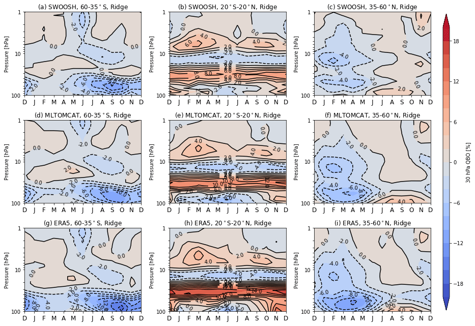
Figure 6 Pressure–season variation in the 30 hPa QBO response in ozone (%) from (a–c) SWOOSH, (d–f) ML-TOMCAT, and (g–i) simulation ERA5 for three selected latitudinal bands (60–35^∘ S, 20^∘ S–20^∘ N, 35–60^∘ N) based on the ridge regression method.

Figure 7 Same as Fig. 6 but for the 50 hPa QBO response in ozone (%).

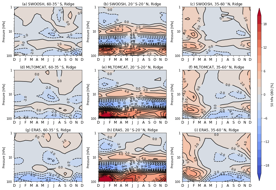
Figure 8 shows the solar cycle response in stratospheric ozone variations derived from SWOOSH, ML-TOMCAT, and simulation ERA5 based on OLS and ridge regression methods. Similarly to the trend results, the coefficients of solar cycle ozone response from ridge regression are relatively small in magnitude. Besides, the OLS-based solar response from SWOOSH data displays a U-shaped structure in the upper stratosphere with maxima stretching from the tropics (5–10 hPa) to mid-latitudes (1–3 hPa). A significant negative peak is observed near 30 hPa in the tropics, which is also found in ML-TOMCAT and simulation ERA5 (although it is not statistically significant). The U-shaped structure in the upper stratosphere is not well reproduced by ML-TOMCAT and simulation ERA5 as the solar cycle ozone response is overestimated at most latitudes and pressure levels, while the locations of the maximum solar responses in the tropics and mid-latitudes are consistent. Differences between the OLS- and ridge-based solar response include (1) the location of the maximum solar cycle ozone response in the tropical upper stratosphere (which is near 3–5 hPa for ridge regression), (2) the location of the negative peak solar response in the tropics (which is up to ∼10 hPa for all datasets in ridge regression), and (3) the significant solar signals near 30–50 hPa in the NH extratropics (which is absent from ridge regression). These features show many similarities as well as differences when compared to those in previous observations and model simulations (Soukharev and Hood, 2006; Maycock et al., 2018; Ball et al., 2019b; Dhomse et al., 2022). The fact is that estimates of a realistic solar cycle signal are challenging as they are not only dependent on the chosen dataset, but also associated with the regression methods, model setup, and proxies used in the MLR analysis (Smith and Matthes, 2008; Chiodo et al., 2014; Ball et al., 2016).

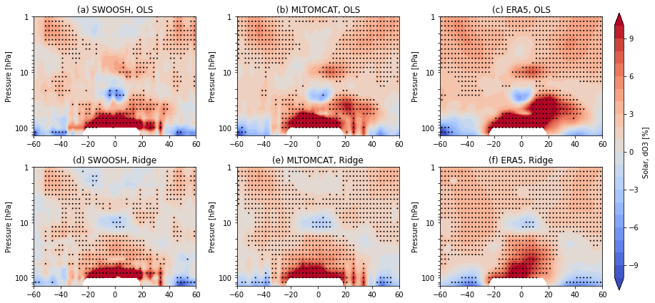
Figure 8 Latitude–pressure cross sections of solar cycle response in stratospheric ozone (%) derived from SWOOSH, ML-TOMCAT, and TOMCAT simulation ERA5 based on (a–c) OLS and (d–f) ridge regression methods. The stippling indicates regions that are significant at the 95 % level.

The solar response in tropical stratospheric ozone (20^∘ S–20^∘ N) is quantified and compared based on different datasets with OLS and ridge regression methods, as shown in Fig. 9. The OLS-based solar response profile from SWOOSH shows a single and broad peak response (2.8 %) at 10 hPa, which is consistent with the results of Ball et al. (2019b). The ridge-based profile shows a different structure with a significant peak signal (1.5 %) near 4.6 hPa and an insignificant negative signal near 10 hPa. In the tropical lower stratosphere there is a secondary ozone peak for both OLS- and ridge-based response, which has been reported in previous studies and is thought to be a dynamical response to the solar cycle (Dhomse et al., 2016). ML-TOMCAT and simulation ERA5 display a consistent structure with SWOOSH although they overestimate the peak response as well as the signals in the upper stratosphere (above 2 hPa). Again, the differences between OLS- and ridge-based solar cycle signal (SCS) profiles indicate that how the MLR model is applied may play a role in the appearance of the solar cycle ozone response (Smith and Matthes, 2008).

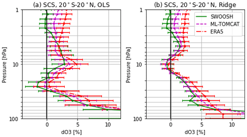
Figure 9 Profiles of ozone solar cycle signal (SCS) for the tropical region (20^∘ S–20^∘ N) from SWOOSH, ML-TOMCAT, and TOMCAT simulation ERA5 based on (a) OLS and (b) ridge regression methods. Error bars are 2σ uncertainties.

In addition, ozone variations associated with natural processes (ENSO, AO, AAO, and EP flux) based on different datasets are shown in Fig. 10 with ridge regression. The ENSO coefficient indicates a significant negative influence on the tropical lower-stratospheric ozone, while there are positive patterns in the northern middle–high latitudes due to enhanced transport from the tropics during warm ENSO events (Frossard et al., 2013; Rieder et al., 2013). In the southern mid-latitudes, the ENSO coefficients are statistically insignificant, implying that ENSO-related ozone variations differ by hemisphere with the ENSO phase (Ziemke et al., 2010; Oman et al., 2013).

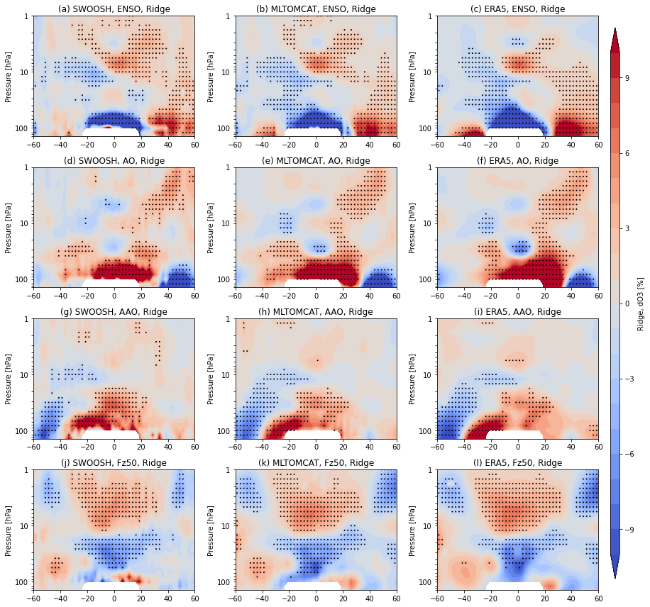
Figure 10 Latitude–pressure cross sections of the natural ozone variations (%) associated with (a–c) ENSO, (d–f) AO, (g–i) AAO, and (j–l) EP flux ($F_{z_{\mathrm{50}}}$) derived from SWOOSH, ML-TOMCAT, and simulation ERA5 based on the ridge regression method. The stippling indicates regions that are significant at the 95 % level.

The negative phase of AO (AAO) in the northern (southern) extratropics leads to increased ozone with enhanced ozone transport (Steinbrecht et al., 2011; Chehade et al., 2014). These negative AO (AAO) indices in the extratropics are characterized by a pronounced poleward deflection of planetary waves, which means an enhanced Brewer–Dobson circulation and more ozone transport into the extratropics (Steinbrecht et al., 2011). As shown in Fig. 10, zonally averaged ozone variations in the lower stratosphere are more sensitive to the AO and AAO indices compared to those in the middle and upper stratosphere.

Changes in the vertical component (F_z) of the stratospheric EP flux represent the ozone transport due to variations in planetary waves driving from the troposphere into the stratosphere (Fusco and Salby, 1999; Weber et al., 2003; Dhomse et al., 2006). In the tropics, the strengthened upward transport is linked to an upward shift in the maximum ozone mixing ratio in the middle stratosphere; as a result there are two cells of opposite ozone pattern near 10 hPa. A similar pattern appears at mid-latitudes due to enhanced transport by the stratospheric residual circulation. The out-of-phase relationship between the tropics and mid-latitudes reflects the overturning Brewer–Dobson circulation (Randel et al., 2002). In the lower stratosphere, the hemispherical asymmetric ozone pattern could potentially result from the combination of changes in chemical and dynamical processes (Banerjee et al., 2016; Abalos et al., 2017).

Both satellite data and model simulation capture these features, although there are still some differences. In the lower stratosphere, simulation ERA5 overestimates the positive ENSO response in the extratropics more than ML-TOMCAT does. In the tropical middle stratosphere near 30 hPa, again ERA5 shows larger AO-related responses than SWOOSH or ML-TOMCAT. Figure S7 shows the results from OLS regression for comparison. With the correction for AR1 applied to OLS regression, the uncertainties in the fit coefficients for these dynamical proxies increase, which makes most of the contributions statistically insignificance. As the correction method can also change the estimated regression coefficients, the differences between OLS- and ridge-based results should be considered with care. As a caveat, the regression fit has been improved by accounting for various dynamical proxies; however, these proxies are not independent and they can only partly explain the complicated structure of dynamical variability (Petropavlovskikh et al., 2019; WMO, 2022). Thus, the use of these dynamical proxies requires care, especially for the lower-stratospheric region.

5 Summary and conclusions

In this study, we have investigated stratospheric ozone trends and their attribution with ordinary (OLS) and regularized (ridge) multivariate regression methods. The merged satellite-based dataset (SWOOSH), TOMCAT model simulation forced with ERA5 reanalysis data, and a machine-learning-based satellite-corrected TOMCAT product (ML-TOMCAT) are used and compared over the period 1984–2020. We adopt the ridge regression method to overcome the issue of over-fitting due to the complex coupling in many atmospheric processes. We have analysed the ozone profile trends and ozone variations associated with natural processes based on both OLS and ridge regression methods. Our main results are summarized as follows:

• As shown in Sect. 4, estimated ozone trends from the OLS- and ridge-based regression models show significant differences. With a penalty considered in ridge regression, coefficients in the regression model are shrunk to a certain extent, which is determined by the optimal tuning value. This optimal tuning value changes with altitude and latitude, indicating, as expected, that ozone concentrations are controlled by different processes at different altitudes and latitudes, and it is inappropriate to use the same tuning value for the ridge regression model for all locations. To avoid over-fitting-related issues, we have applied ridge regression to quantify the stratospheric ozone trends and changes and to compare it with the conventional OLS regression method.

• We compare the stratospheric ozone profile trends for the pre- and post-1998 periods as well as the seasonal dependence with OLS and ridge regression. Both OLS and ridge regression methods show a strong seasonal dependence in stratospheric ozone trends. Trend estimates at different altitudes and seasons are constrained by ridge regression in magnitudes and fluctuations. For example, ozone declines during 1984–1997 are smaller in ridge regression, and the largest differences between ozone trends using OLS and ridge regression are apparent in the upper stratosphere (∼1 % per decade at 2 hPa) and the lowermost stratosphere (>4 % per decade at 100 hPa) for SWOOSH data. From 1998, all the datasets confirm stratospheric ozone recovery in the upper stratosphere, but there are differences in the magnitudes and the locations. In the NH mid-latitudes and the tropics, the largest positive trends are observed at 2 hPa (1.1±1.1 % per decade and 1.1±1.0 % per decade, respectively). On the other hand, positive trends are somewhat larger at SH mid-latitudes (1.3±0.8 % per decade) though they occur at 3.8 hPa. Negative trends with large uncertainties are observed in the lower stratosphere and are most pronounced in the tropics. The largest difference between OLS and ridge regression methods appears in the tropical lower stratosphere (with ∼9 % per decade difference at 100 hPa), but it is within the uncertainties of the individual trends (>10 % per decade). Comparing trend estimates from TOMCAT model simulation, we find that ML-TOMCAT trends are more consistent with those using SWOOSH data. The differences between satellite-based datasets and model simulations suggest there are still large uncertainties in the lower stratosphere where dynamical processes dominate.

• Ozone variations associated with natural processes such as QBO, solar variability, ENSO, AO, AAO, and EP flux indicate that ridge regression shrinks the regression coefficients as some of the explanatory variables are co-related. The differences between OLS- and ridge-based results are associated with how the MLR model is applied and should be considered with care. Despite the differences in regression coefficients and statistical significance, there are similar characteristics in natural ozone variations for both regression methods. For example, the positive QBO influences on the tropical lower-stratospheric ozone and negative influences in the subtropical region are consistent with QBO signals in total column ozone. The stratospheric ozone solar cycle response shows a U-shaped spatial structure in the upper stratosphere. The enhanced transport from the tropics during warm ENSO events leads to a significant negative influence on the tropical lower-stratospheric ozone and positive influences in the northern middle–high latitudes. The negative phase of AO/AAO in the northern/southern extratropics leads to increased ozone with enhanced ozone transport. The stratospheric EP flux represents planetary waves driving from the troposphere into the stratosphere and affects the ozone transport through Brewer–Dobson circulation. Again, ML-TOMCAT shows more consistent results with those using SWOOSH data, while simulation ERA5 shows larger inconsistencies, especially in the lower stratosphere.

Finally, we argue that the considerable differences between the satellite data and model simulations highlight the large uncertainties in our understanding about the lower-stratospheric trends, which suggests that caution is needed while interpreting results with different methodologies and datasets.