Changes in surface ozone in South Korea on diurnal to decadal timescales for the period of 2001–2021

Several studies have reported an increasing trend of surface ozone in South Korea over the past few decades, using different measurement metrics. In this study, we examined the surface ozone trends in South Korea by analyzing the hourly or daily maximum 8 h average ozone concentrations (MDA8) measured at the surface from 2001 to 2021. We studied the diurnal, seasonal, and multi-decadal variations of these parameters at city, province, and background sites.

We found that the fourth-highest MDA8 values exhibited positive trends in seven cities, nine provinces, and two background sites from 2001 to 2021. For the majority of sites, there was an annual increase of approximately 1–2 ppb. After early 2010, all sites consistently recorded MDA8 values exceeding 70 ppb, despite reductions in precursor pollutants such as NO₂ and CO. The diurnal and seasonal characteristics of ozone exceedances, defined as the percentage of data points with hourly ozone concentrations exceeding 70 ppb, differed between the Seoul Metropolitan Area (SMA) and the background sites.

In the SMA, the exceedances were more prevalent during summer compared to spring, whereas the background sites experienced higher exceedances in spring than in summer. This indicates the efficient local production of ozone in the SMA during summer and the strong influence of long-range transport during spring. The rest of the sites showed similar exceedance patterns during both spring and summer. The peak exceedances occurred around 16:00–17:00 in the SMA and most locations, while the background sites primarily recorded exceedances throughout the night.

During the spring of the COVID-19 pandemic (2020–2021), ozone exceedances decreased at most locations, potentially due to significant reductions in NO_x emissions in South Korea and China compared to the period of 2010–2019. The largest decreases in exceedances were observed at the background sites during spring. For instance, in Gosung, Gangwondo (approximately 600 m above sea level), the exceedances dropped from 30 % to around 5 % during the COVID-19 pandemic.

Regional model simulations confirmed the concept of decreased ozone levels in the boundary layer in Seoul and Gangwon-do in response to emission reductions. However, these reductions in ozone exceedances were not observed in major cities and provinces during the summer of the COVID-19 pandemic, as the decreases in NO_x emissions in South Korea and China were much smaller compared to spring. This study highlights the distinctions between spring and summer in the formation and transport of surface ozone in South Korea, emphasizing the importance of monitoring and modeling specific processes for each season or finer timescales.

1 Introduction

Ozone, a greenhouse gas and harmful air pollutant, can accumulate in the lower atmosphere through photochemical reactions involving nitrogen oxides and volatile organic compounds from both human activities and natural sources (National Research Council, 1991; Monks et al., 2015). The increasing concentrations of ozone near the surface and in the troposphere are concerning. Gaudel et al. (2018) reported a significant increase in ozone levels in South Korea from 2000 to 2014, while North America and Europe experienced decreasing trends, using data from surface monitors, ozonesondes, and aircraft observations. Other studies have also observed rising ozone trends in South Korea between 2001 and 2018 in their analysis of the long-term variations of multiple pollutants over Seoul (Kim and Lee, 2018) and South Korea (Kim et al., 2018) or in the reviews of current status and future directions of tropospheric ozone studies in South Korea (Lee et al., 2020) or in the trend estimates of the surface ozone observations (Yeo and Kim, 2021). Ozone in South Korea can be influenced by ozone and its precursors in China (Oh et al., 2010; Lee and Park, 2022; Colombi et al., 2023). However, Gaudel et al. (2018) did not include Chinese data due to a lack of reported information. Recent studies have highlighted a rapid increase in ozone levels in China from 2004 to 2020, especially after 2013 (Li et al., 2019; Wang et al., 2020, 2022). Gaudel et al. (2020) also found that tropospheric ozone in China and South Korea increased between 1996 and 2016. Considering the proximity of the two countries and their potential for ozone and precursor exchange, it is essential to study the ozone trends in South Korea in relation to those in China. Additionally, as spring and summer have distinct transport patterns and source–receptor relationships relevant to surface and tropospheric ozone (e.g., Cooper et al., 2010), it would be valuable to investigate ozone trends separately for these seasons.

The COVID-19 pandemic brought about significant changes in atmospheric composition (Bauwens et al., 2020; Koo et al., 2020; Seo et al., 2021). Analyzing deviations from long-term trends during the pandemic can provide valuable insights for future environmental policies aimed at mitigating ozone pollution. In this study, we examine ozone trends and exceedances in South Korea from 2001 to 2021, focusing on the warm seasons of spring and summer, including the COVID-19 period. In this study, we analyzed the fourth-highest daily maximum 8 h average ozone concentrations (MDA8 O₃) at various locations in South Korea for a global comparison because this is a metric used for the US Environmental Protection Agency National Ambient Air Quality Standard, and the recent study by Wang et al. (2022) utilized the same metric for their study of Chinese ozone pollution. We also introduced a new metric of ozone exceedance, defined as the percentage of data points with hourly ozone concentrations exceeding 70 ppb. Previous published works about surface ozone in South Korea have not focused on the two metrics used in our study. We analyze diurnal, seasonal, and decadal variations at seven cities, nine provinces, and two background sites. Furthermore, we discuss the factors contributing to the observed temporal changes based on regional model results.

The paper is organized as follows. In Sect. 2, the surface and satellite data, global and regional modeling, and other methods to utilize the data are explained. In Sect. 3, the results are summarized as long-term trends of ozone and its precursors, characteristics of diurnal variations, and spatiotemporal variations during the pandemic. The regional model results based on various emission scenarios are also shown to identify the source–receptor relationship. Finally, the results are summarized, and future research directions are suggested in the conclusions.

2 Data and method

2.1 Long-term surface observational data

The hourly surface air quality monitoring data are obtained from the Airkorea website (NIER, 2022), including ozone (O₃), NO₂, SO₂, CO, PM₁₀, and PM_2.5 (PM_2.5 data are provided for 2015 onwards). As of March 2020, there were about 500 monitoring stations over South Korea. These routine monitor data are available for many decades and can serve as a main dataset to examine long-term trends. We utilized hourly and daily maximum 8 h average O₃ concentrations. The surface monitoring sites used in this study and the data availability are summarized in the Supplement 1 (Table S1) and Supplement 2. O₃, NO₂, and CO data are also averaged for spring and summer months. These surface monitoring data were used to investigate the impact of the COVID-19 pandemic in the Seoul Metropolitan Area (SMA).

2.2 Highway toll number and mobile phone usage data

To examine changes in mobility pattern during the COVID-19 pandemic, traffic counts from the Korea Expressway Corporation daily transit data were used (Korea Expressway Corporation, 2023). The expressway transit data covering 3 years (2019–2021) of traffic passing toll gates were quantified from Hi-Pass (electronic toll collection system) and cash toll collection. Vehicles passing toll gates were not classified in detail.

To examine changes in mobility pattern during the COVID-19 pandemic, daily mobile phone movement provided by Android (Google, 2022) and Apple (Apple, 2022) are used. Android mobility data tracked movements of people using cell phones at the same spot, while Apple's mobility report collects personal vehicle routing requests from Apple Maps. For Google and Apple mobility reports, we used the transit station mobility metrics and driving mobility index in the Seoul Metropolitan Area, respectively. The reports must be used carefully as they do not directly quantify on-road traffic.

2.3 Satellite data: tropospheric NO₂ columns

The TROPOspheric Monitoring Instrument (TROPOMI) is on board a low Earth polar orbiting satellite, the European Space Agency (ESA) Sentinel-5 Precursor (S-5P) satellite, with an Equator passing time of 13:30 local time. The instrument provides measurements at unprecedentedly high spatial, temporal, and spectral resolutions (Veefkind et al., 2012). In this study we utilized two available tropospheric NO₂ datasets from TROPOMI, NASA's standard product (SP) version 4.0 (Lamsal et al., 2021, 2022) and KNMI's (Royal Netherlands Meteorological Institute) product obtained from DOMINO v2.0 and QA4ECV v1.1 (Derivation of TROPOMI tropospheric NO₂) processing systems (Boersma et al., 2018; KNMI, 2021). The spatial resolution of KNMI's tropospheric NO₂ retrieval product is 3.5 km × 7 km (3.5 km × 5.5 km since 6 August 2019), and that of NASA's product is 3.5 km × 5.5 km. Level 2 data with pixels passing quality assurance > 0.75 and the cloud fraction < 0.5 were selected for analysis following recommendations provided by Sentinel-5 precursor TROPOMI Level 2 Product User Manual for nitrogen dioxide (Eskes et al., 2019). TROPOMI data are regridded to a standard grid with a horizontal resolution of 0.1^∘ latitude × 0.1^∘ longitude (11 × 11 km), and monthly averaged values were derived. As the random error in the TROPOMI single-pixel uncertainties influence 40 % to 60 % of the tropospheric column abundance, temporal and spatial averaging may remove the random errors (Bauwens et al., 2020).

We conducted the sensitivity test by applying different sampling conditions and found consistent results irrespective of quality control parameters: larger tropospheric NO₂ column reduction during spring than during summer between 2019 and 2020–2021 (COVID-19 periods). Differences between KNMI and NASA retrievals are large when the filtering condition of quality assurance > 0.5 and cloud radiance fraction < 0.4 is applied. When the stricter filter is applied, differences between KNMI and NASA retrievals are small. Therefore, the stricter filter (quality assurance > 0.75 and cloud radiance fraction < 0.5) is selected. Since the NASA product released in November 2022 was generated in a consistent manner for May 2018–December 2021, we mainly present the NASA product. We summarize the sensitivity tests in the Supplement 3. The distribution of absolute tropospheric NO₂ columns for different years is also shown in the Supplement 3.

2.4 CAM-Chem model simulations

The atmospheric component of the Community Earth System model (CESMv2.2), the Community Atmosphere Model with Chemistry version 6 (CAM6-chem), is developed by the National Center for Atmospheric Research (NCAR) (NCAR, 2020). The CAM-Chem adapted MOZART-T1 as the tropospheric chemistry mechanism (Emmons et al., 2020). The simulation used in this study was configured with 1^∘ horizontal resolution. The sea surface temperature was prescribed, and meteorological fields were nudged to Modern-Era Retrospective analysis for Research and Applications version 2 (MERRA-2) instead of using a self-produced meteorological field (https://gmao.gsfc.nasa.gov/reanalysis/MERRA-2/, last access: 23 May 2022) (refer to Supplement 1 Fig. S1 for performance of the model wind). The simulation was performed from 2000 to 2020 and applied the CMIP6 emission inventory (2000–2014) and SSP5-8-5 emission inventory (2015–2020). The first 3 years was regarded as a spin-up. In this study, we utilized the CAM-Chem results to estimate the impact of stratospheric ozone on the surface in each season. CAM-Chem calculates the contribution of stratospheric ozone to tropospheric ozone, O_3S, as a three-dimensional variable in space. Originally, O_3S is an ozone value above the tropopause. Then O_3S is transported below tropopause and undergoes chemical losses in the model. Evaluations of the CAM-Chem results against the data from the ozonesondes that were launched in Pohang, South Korea, are shown in the Supplement 1 (Fig. S2; Jeong et al., 2023). The model results and observations reasonably agree in terms of seasonal variability and absolute values. In particular, the CAM-Chem results agree with the observations at the 200 hPa level, close to tropopause.

2.5 WRF-Chem model simulations

The Weather Research and Forecasting (WRF) model coupled with Chemistry (WRF-Chem) is developed by National Oceanic and Atmospheric Administration (NOAA) and National Center for Atmospheric Research (NCAR) and collaborating institutes (Grell et al., 2005; NCAR, 2022). We utilized WRF-Chem v4.4 to simulate regional meteorological fields and chemical compositions.

Our WRF-Chem setup utilizes the horizontal resolution of 28×28 km² and 60 vertical levels. The simulation period is from 24 April 12:00 UTC to 11 June 12:00 UTC in 2016. We restart the simulation at 12 UTC every day to reduce computing errors. The first 7 d of model simulation is regarded as the spin-up period. The analysis period is selected as 1 May to 10 June based on local time. The Global Forecast System (GFS) Final (FNL) analysis data are used for meteorological input and boundary conditions (https://rda.ucar.edu/datasets/ds083.2/). We used the Community Atmosphere Model with Chemistry (CAM-Chem) output to the chemical boundary and first initial conditions (https://www.acom.ucar.edu/cam-chem/cam-chem.shtml, last access: 25 July 2022) (Buchholz et al., 2019). The Model of Emissions of Gases and Aerosols from Nature (MEGAN) is used for biogenic emissions (Guenther et al., 2006).

There are seven model sensitivity runs that adopt different emission scenarios. The control run is based on the standard EDGAR-HTAPv3 emission inventory representing 2016 (Crippa et al., 2023). Park et al. (2021) established that biomass burning was not an important factor affecting air quality in South Korea during KORUS-AQ. Therefore, biomass burning emissions are omitted in this study. The “No China” case removes all anthropogenic emissions in China. The “No Seoul” case eliminates all anthropogenic emissions in Seoul. There is one case that decreased Chinese volatile organic carbon (VOC) emissions by 50 %. There are two cases that reduced Chinese NO_x emissions by 50 %: one case has the same VOC emissions as in the control case, while the other case has the 50 % reductions of VOC emissions as well. Lastly, there is one case that reduced Chinese NO_x emissions by 75 %. The WRF-Chem sensitivity runs are summarized and are discussed in Sect. 3. The extensive evaluations of the model results against the surface and airborne data from the KORUS-AQ field campaign (NASA, 2019) in 2016 are shown in the Supplement 1 (Tables S2–S4 and Figs. S3–S8) and Kim et al. (2023). More discussions about all bottom-up emission inventories utilized for the WRF-Chem simulations and comparison of those with the emissions used for the CAM-Chem simulations are included in the Supplement 1 Table S5.

3 Results

3.1 Surface ozone trends

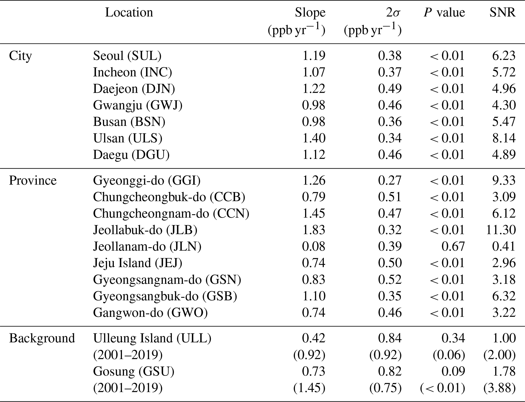
In this study, ozone and its precursor concentrations in seven cities, nine provinces, and two background sites in South Korea (Fig. 1) are analyzed at diurnal, seasonal, and decadal timescales. Figure 2 and 3 show the fourth-highest daily maximum 8 h average ozone concentrations (MDA8 O₃) for the cities and provinces for ozone season (May–September) from 2001 to 2021. The results from statistical analysis (slope, standard deviation, p value, signal-to-noise ratio) are summarized in Table 1. P values were presented as suggested by Chang et al. (2021) and Wasserstein et al. (2019) for the purpose of estimating uncertainties in trends. The fourth-highest MDA8 O₃ increases by 1.0–1.5 ppb yr⁻¹ with very high certainty for most of cities and provinces across South Korea in this period. In nearly all cities and provinces, the fourth-highest MDA8 O₃ has been higher than 70 ppb since 2010 or earlier (see dashed gray line in Figs. 2 and 3). The trend in Jeollanam-do (JLN) is small with very low certainty (p= 0.67), partly because the MDA8 O₃ was high before 2010. The monitoring sites in Jeollanam-do include the Yeosu-Kwangyang region in which many petrochemical industries and iron steel complexes are located. This region experienced severe ozone problems in the 1990s to early 2000s (Ghim, 2000). Because of discontinuity of data records, the background sites are omitted in the trend analysis in Figs. 2 and 3. Although there are missing data during the ozone season for the background sites, we estimated the trends of the fourth-highest MDA8 O₃ for a reference (Table 1). The estimated trend for Ulleung Island is 0.42 ppb yr⁻¹ from 2001 to 2021 with low or very low certainty. The trend for Ulleung Island increases to 0.92 ppb yr⁻¹ for 2001–2019 with medium certainty. The estimated trend for Gosung is 0.73 ppb yr⁻¹ from 2001 to 2021 with medium to high certainty. The trend for Gosung increased to 1.45 ppb yr⁻¹ for 2001–2019 with very high certainty. Widely increasing long-term ozone trends in South Korea indicate a regional nature of this pollutant, potentially influenced by East Asian emissions, chemical transformations, and long-range transport (Colombi et al., 2023; Lee and Park, 2022). Therefore, it is imperative to understand the local and regional processes that enhance surface ozone. Ozone originated from Asia is known to be efficiently transported to North America during springtime (Jacob et al., 1999; Jaffe et al., 1999, 2003; Cooper et al., 2010; Lin et al., 2012; Langford et al., 2017; Jaffe et al., 2018) and summertime (Fiore et al., 2002; Liang et al., 2007) as well. Investigating seasonal differences in ozone in South Korea may provide insights into the relative importance of local and regional processes.

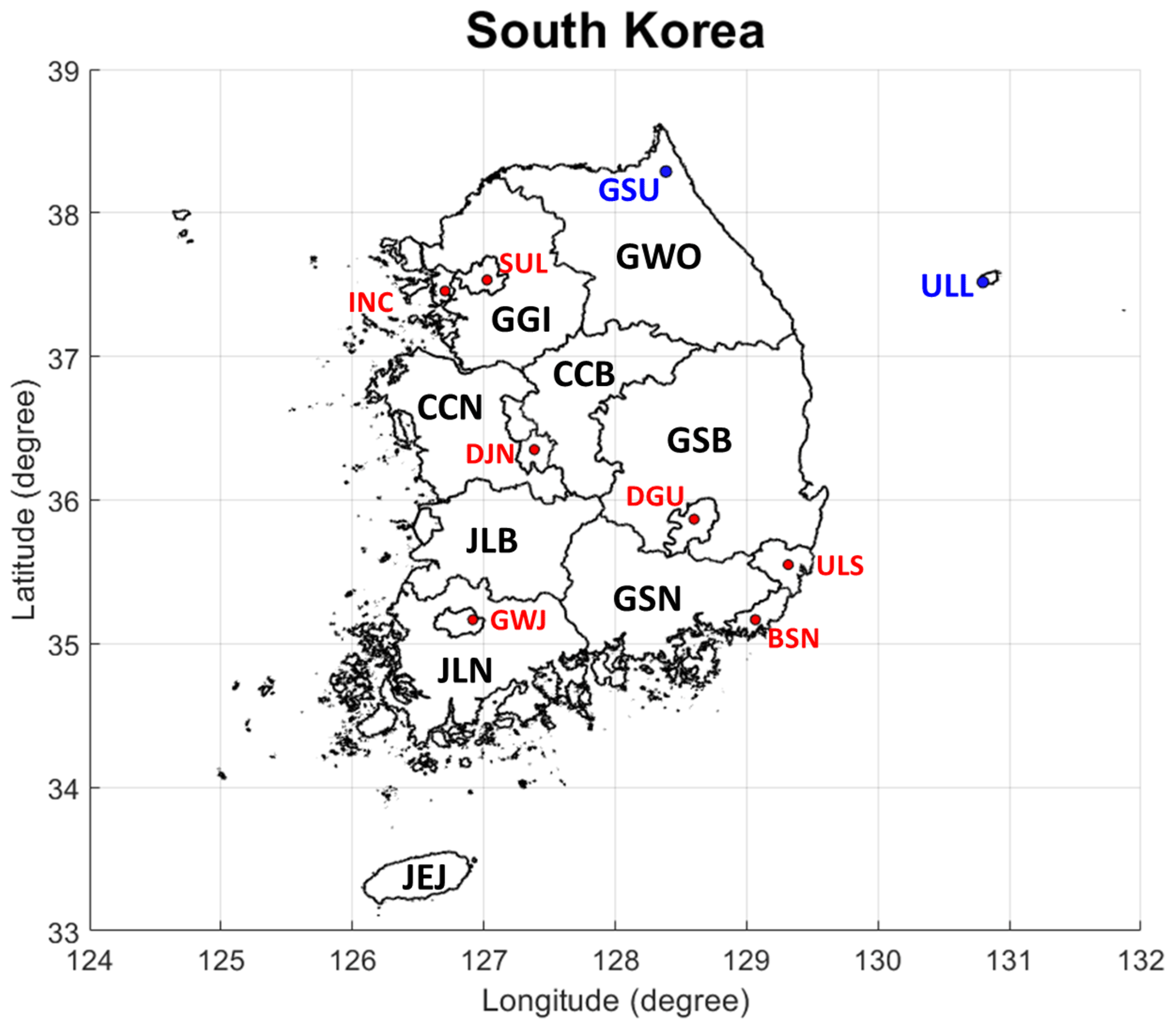
Figure 1 The locations of cities, provinces, and background sites in South Korea. The red, black, and blue colors denote city, province, and background sites, respectively. Cities – SUL (Seoul), INC (Incheon), DJN (Daejeon), GWJ (Gwangju), BSN (Busan), ULS (Ulsan), and DGU (Daegu). Provinces – GGI (Gyeonggi-do), CCB (Chungcheongbuk-do), CCN (Chungcheongnam-do), JLB (Jeollabuk-do), JLN (Jeollanam-do), JEJ (Jeju Island), GSN (Gyeongsangnam-do), GSB (Gyeongsangbuk-do), and GWO (Gangwon-do). Background sites – ULL (Ulleung Island) and GSU (Gosung, Gangwon-do).

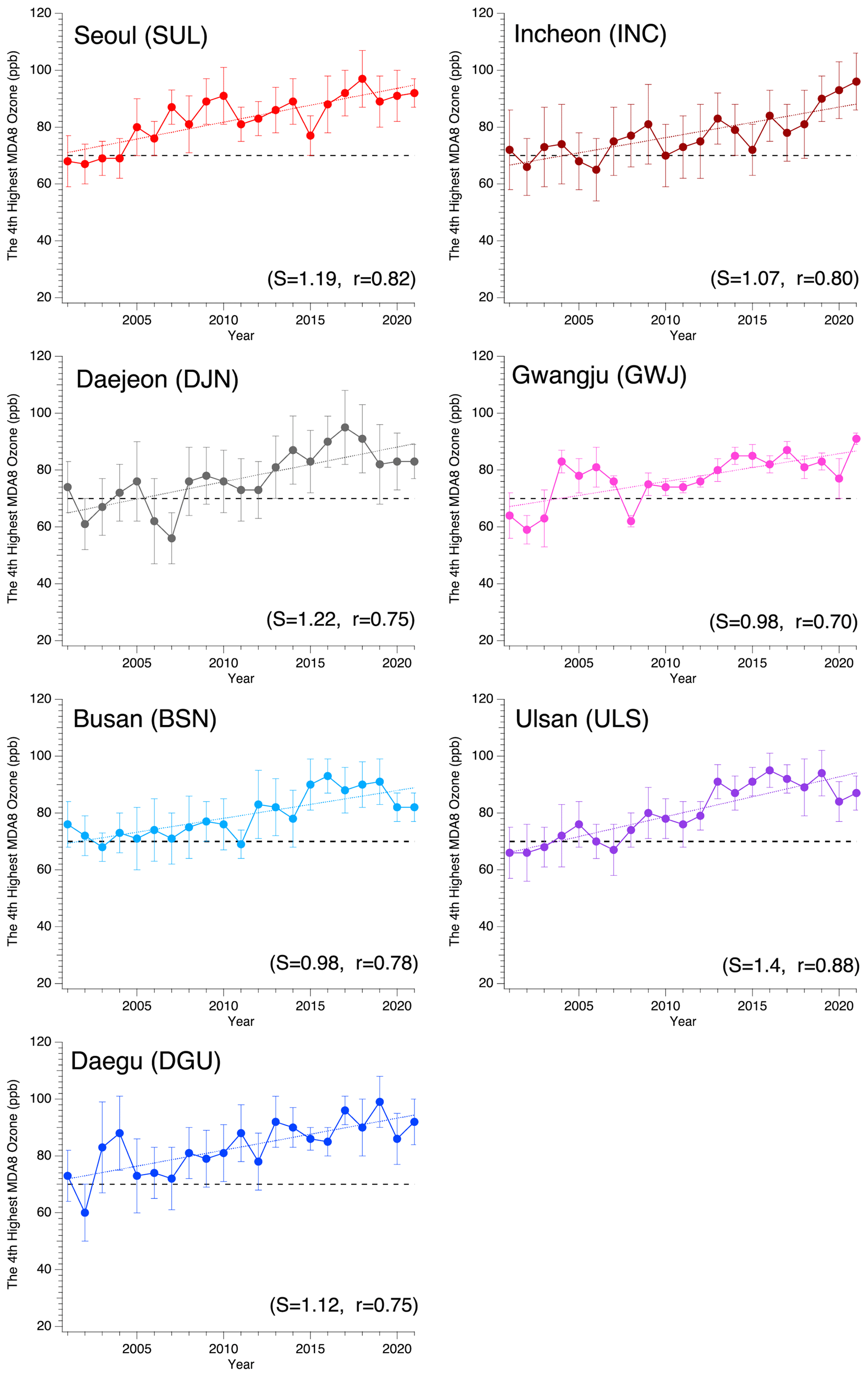
Figure 2 The trend of the fourth-highest daily maximum 8 h average (MDA8) O₃ concentrations in the South Korean metropolitan cities from 2001 to 2021. Only the data for May–September (ozone season) are used. Bars denote standard deviations among the sites within the city. The slopes (S) and correlation coefficient (r) from linear fits are shown in parentheses. The dashed gray line indicates 70 ppb, which is the air quality standard defined by the US Environmental Protection Agency.

Figure 3 The same as in Fig. 2 except for South Korean provinces.

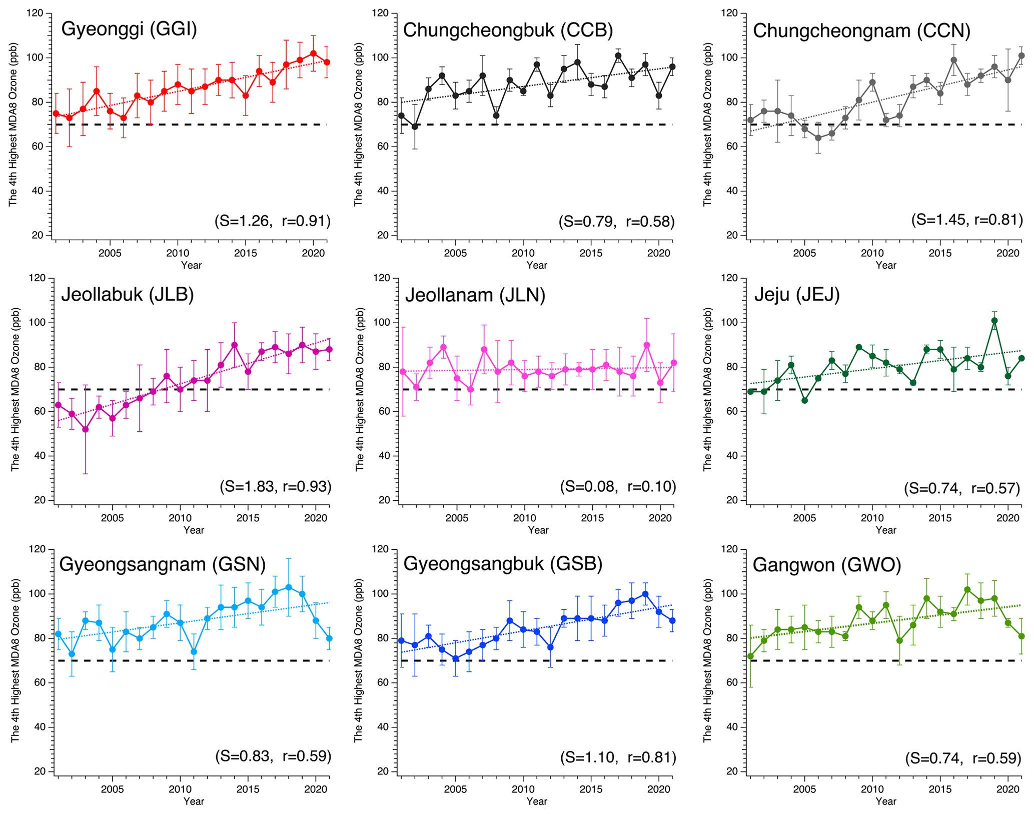
Table 1 Trend estimates based on the fourth-highest MDA8 O₃ values from 2001 to 2021. The data were acquired from the surface monitoring network (NIER, 2022). The unit of the slope and limit (2σ=2 standard deviations) is parts per billion per year (ppb yr⁻¹). SNR denotes the signal-to-noise ratio, defined as the ratio of the absolute value of the slope to standard deviation. For the use of P value and SNR, refer to Chang et al. (2021). Data during a typical ozone season (May–September) are analyzed. Some data for the background sites are missing (refer to Supplement 2).

3.2 Difference between spring and summer: background value, exceedance, stratospheric influence, and precursor concentrations

3.2.1 Background values in the daytime and nighttime periods

Table 2 summarizes the abundances and differences between spring and summer ozone concentrations averaged for the daytime (10:00–20:00 local time (LT)) and the nighttime (01:00–06:00 LT) periods. Standard deviations denoting year-to-year variability are also shown in the table. For the nighttime period, the averaged ozone concentration in spring is always higher than that in summer: differences between the two seasons range from 3.3 to 15.4 ppb and are generally larger than standard deviations. The differences for the background sites are approximately 13 ppb at this time. This clearly indicates the importance of large-scale influences in spring. The results are the same for the daytime period except for Seoul and Gyeonggi-do: the mean ozone concentrations in Seoul and Gyeonggi-do in summer are slightly higher than those in spring. The differences in the daytime period are small for Incheon, Daegu, and Chungcheongbuk-do, suggesting the importance of local chemistry in the areas during summer. Overall, standard deviations are larger than the differences in the daytime period except Busan, Jeollanam-do, Jeju Island, Gyeongsangbuk-do, Gangwon-do, and the background sites. The differences for the background sites in the daytime period are approximately 13–15 ppb, which are similar to the values in the nighttime period.

Table 2 Spring and summer ozone concentrations in South Korean metropolitan cities and provinces. Both daytime (10:00–20:00 LT) and nighttime (01:00–06:00 LT) averages are shown. Standard deviations (SDs) denoting year-to-year variability are shown in the parentheses. Differences in concentrations between spring and summer (O_3 spring–O_3 summer) are in square brackets. The cities and provinces listed in the table are in a counterclockwise order with regards to the South Korean map. The data from 2002 to 2019 are utilized.

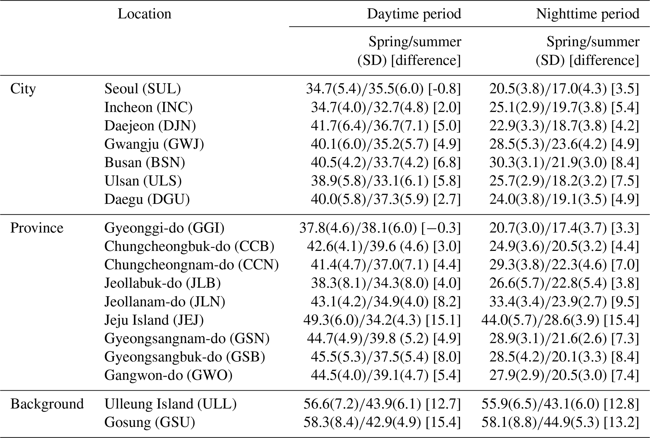
The surface ozone data for 01:00–06:00 LT over polluted regions are often omitted in the analysis because ozone loss reacting with NO is an important process to control ozone levels at nighttime. In this study, we utilized the ozone data at this time to find information about background ozone because ozone is transported throughout a day and this process is essential in the studied region. WRF-Chem sensitivity runs demonstrated an increase in ozone from upwind sources at this time (refer to Supplement 1 Fig. S9).

Additionally, we also calculated O_x (i.e., O₃ + NO₂) that is not affected by the reaction of ozone with fresh local NO_x emissions during nighttime and compared this value at daytime and nighttime for each season (Supplement 1 Tables S6 and S7 for NO₂ and O_x, respectively). Overall, O_x during spring is higher than that during summer, and nighttime differences are prominent, which is similar to the conclusions from the analysis of O₃.

3.2.2 Ozone exceedances

Figure 4 illustrates the ratio of summer ozone exceedances to spring ozone exceedances for the cities, provinces, and background sites. In Seoul, Incheon, and Gyeonggi-do, there are more exceedances in summer than in spring, indicating the significance of local ozone production during the summer season in these areas. Conversely, at the background sites such as Gosung and Ulleung Island, springtime exceedances dominate, highlighting the importance of high springtime ozone levels and their transport within and beyond Asia. For the remaining regions, springtime and summertime exceedances are comparable, or springtime exceedances are slightly higher than those in summer. Note that meteorological conditions in Seoul and Gyeonggi-do (differences between the two seasons) are similar to other cities and provinces (see Supplement 1 Table S8). Therefore, the meteorological factors are not the main drivers of high summertime exceedances in the Seoul and Gyeonggi-do region.

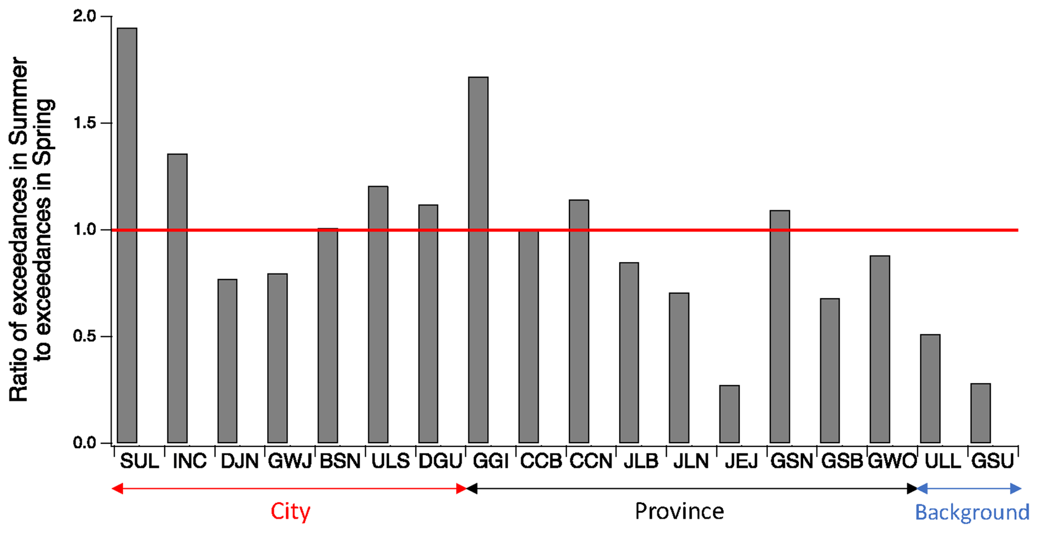
Figure 4 Ratio of O₃ exceedances in summer to exceedances in spring. The exceedances are defined as the fraction of the data with hourly ozone concentration greater than 70 ppb among all available data. The red line indicates a 1 : 1 line. The x axis denotes names of cities, provinces, and background sites. Cities – SUL (Seoul), INC (Incheon), DJN (Daejeon), GWJ (Gwangju), BSN (Busan), ULS (Ulsan), and DGU (Daegu). Provinces – GGI (Gyeonggi-do), CCB (Chungcheongbuk-do), CCN (Chungcheongnam-do), JLB (Jeollabuk-do), JLN (Jeollanam-do), JEJ (Jeju Island), GSN (Gyeongsangnam-do), GSB (Gyeongsangbuk-do), and GWO (Gangwon-do). Background sites – ULL (Ulleung Island) and GSU (Gosung, Gangwon-do). The data for 2002–2019 are utilized.

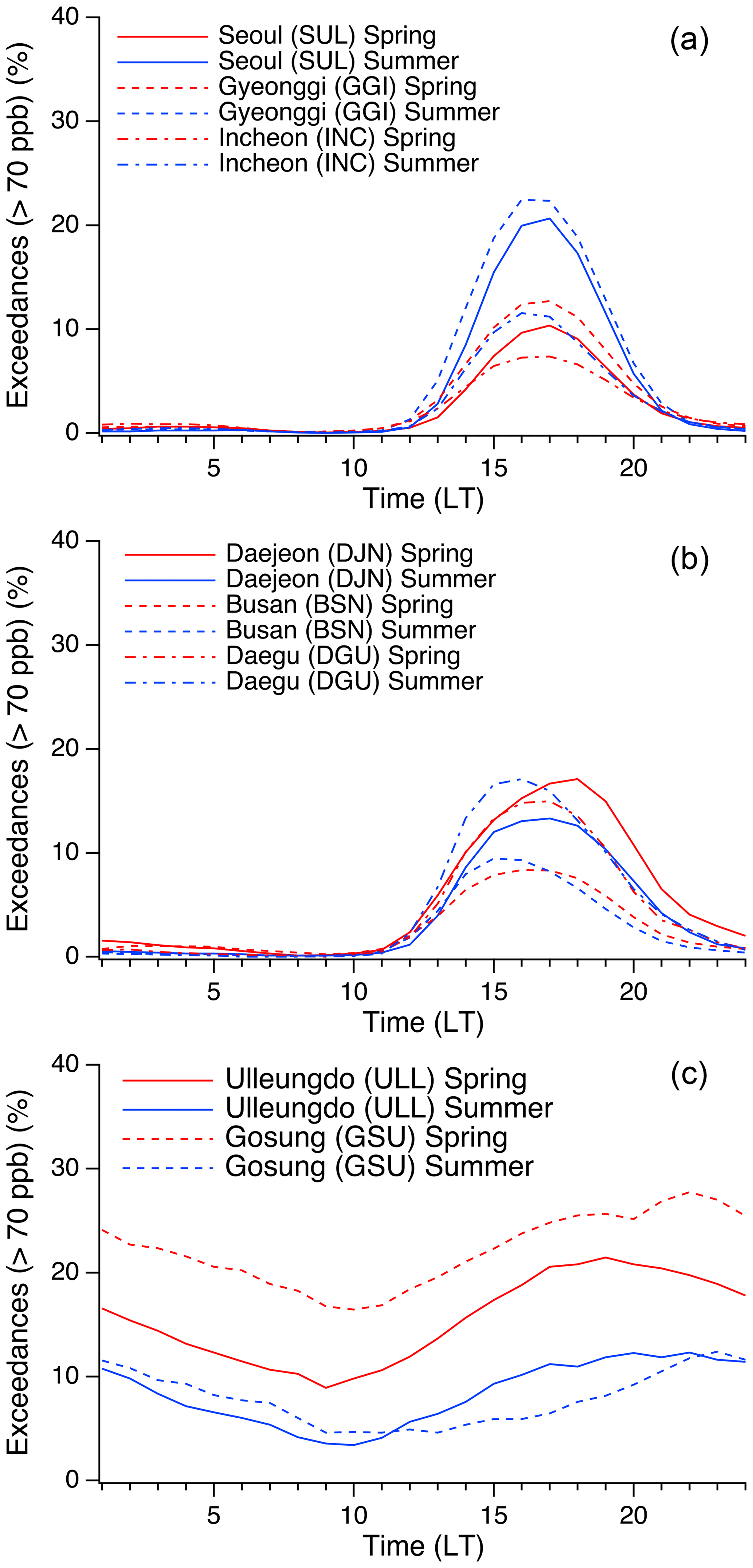
Figure 5 Diurnal O₃ exceedances over selected sites. (a) cities and province in the Seoul Metropolitan Area, (b) other cities, and (c) background sites. The data for 2002–2019 are utilized.

The diurnal variations of exceedances, as shown in Fig. 5, confirm these findings. The summertime ozone exceedances are notably enhanced during the daytime, from 13:00 to 20:00 local time (LT), suggesting efficient photochemical ozone production during this season. The peak exceedances occur at 17:00 LT in Seoul and Gyeonggi-do, and 1 h earlier at 16:00 LT in Incheon. Incheon, being situated adjacent to the Yellow Sea (as depicted in Fig. 1), experiences airflow from Incheon to Seoul under typical westerly or sea breeze conditions. The late-afternoon peaks (16:00–17:00) in the region and the 1 h delay in peak exceedances in Seoul compared to the time of exceedances in Incheon imply that local circulation plays a significant role in the buildup and distribution of ozone within the Incheon, Seoul, and Gyeonggi-do region.

Springtime and summertime ozone exceedances predominantly occur during the daytime, with some extent of exceedances at night, in Daejeon, Busan, and Daegu (Fig. 5). Notably, the peaks in spring occur approximately 2 h later than those in summer for the three cities, indicating a potential influence of transport during the spring season. Negligible exceedances are observed from midnight to 10:00 LT in the three cities due to high NO_x pollution and the depletion of ozone associated with NO_x during this time period.

At the background sites, springtime exceedances are much higher compared to summer, and nighttime exceedances are as frequent as daytime exceedances. In Gosung, springtime exceedances account for approximately 20 % of the observations throughout the day, whereas summertime exceedances are less than or equal to 10 % (Fig. 5). The observation site in Gosung is located at an altitude of approximately 600 m above sea level, providing a unique opportunity to examine long-range-transported plumes and background information at higher altitudes (refer to Supplement 1 Tables S9 and S10). Diurnal variations of exceedances during spring and summer for all individual sites are illustrated in Supplement 1 (Figs. S11–S13).

3.2.3 Influence of stratospheric ozone

Stratospheric ozone can deeply intrude into the lower troposphere, leading to elevated surface ozone levels, particularly during the spring season (Lin et al., 2012, 2015). It is important to assess the contribution of stratospheric ozone to surface ozone in South Korea and understand its potential impact on surface ozone trends in the region using results from the CAM-Chem model. The derivation of the contribution of stratospheric ozone in the CAM-Chem is explained in Supplement 1. Figure 6 presents the contribution of stratospheric ozone to surface ozone in South Korea for each season. According to our global chemistry–climate model simulations, stratospheric ozone has the greatest influence on surface ozone during winter and spring, increasing levels by 17–23 ppb. The model suggests that approximately 37 % and 76 % of surface ozone in spring and winter, respectively, can be attributed to stratospheric ozone (refer to Supplement 1 Table S10 for summary of the CAM-Chem results for all seasons at surface and 1 km above ground level). However, during the summer season, the impact of stratospheric ozone on surface ozone is minimal, accounting for only around 4 % of the surface ozone concentration. Therefore, it would be valuable to analyze ozone trends and exceedances separately for spring and summer. It is worth noting that the contribution of stratospheric ozone to surface ozone does not exhibit clear trends during the period from 2001 to 2021 (not shown). Note that the contribution of stratospheric ozone to tropospheric ozone at each altitude and time shown in this study should be a qualitative measure since the representation of this process has uncertainties and needs further assessment.

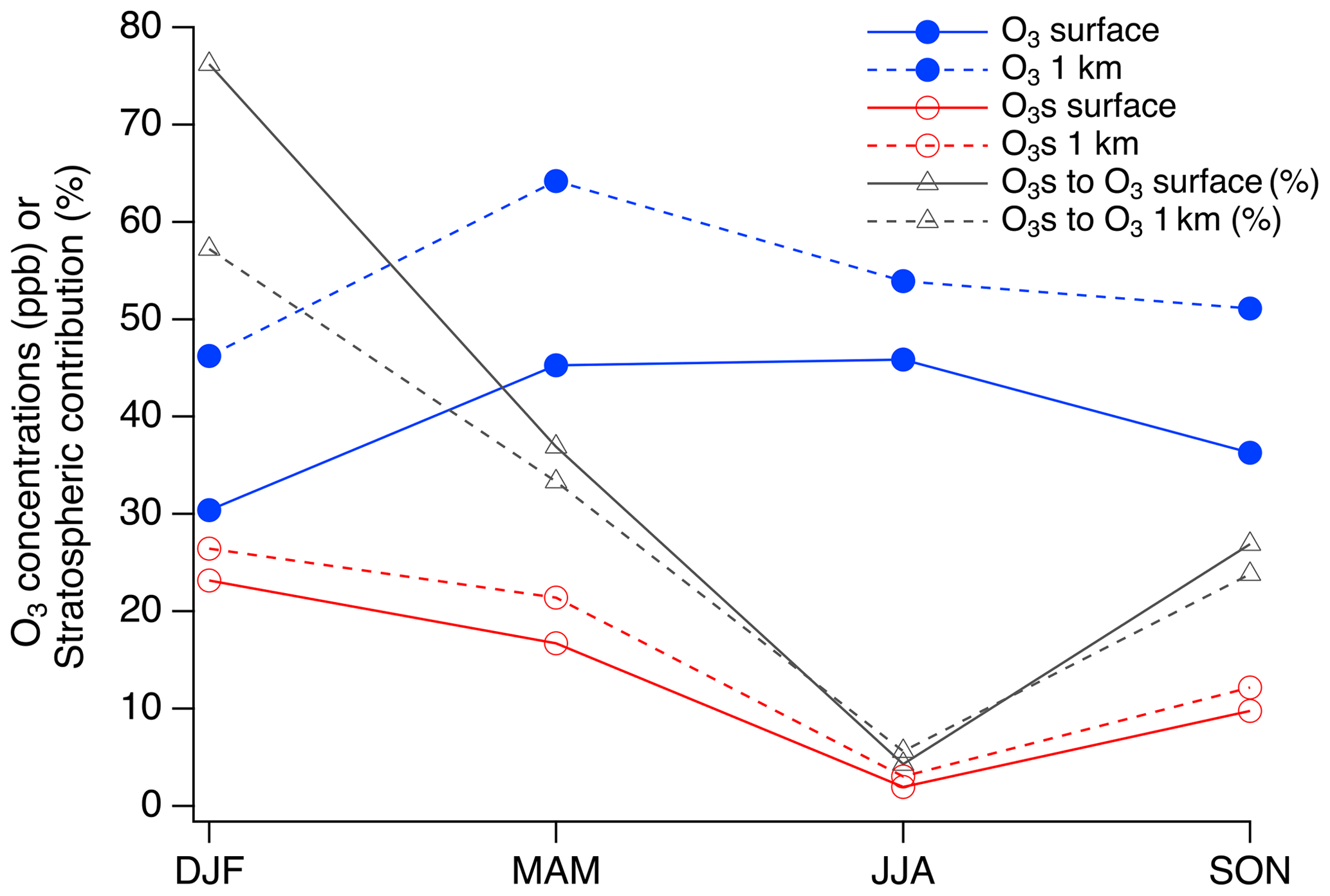
Figure 6 The contribution of stratospheric O₃ (O_3S) to the O₃ concentrations in each season at surface and 1 km above ground level in South Korea. The plotted values are extracted from the CESMv2.2 results for the entire country.

3.2.4 Long-term trends of surface NO₂ and CO concentrations

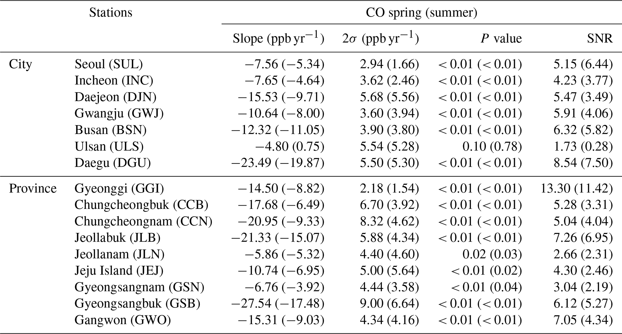
In contrast to the trends of ozone, NO₂ and CO that are ozone precursors decreased both in spring and summer from 2001 to 2021 (Tables 3 and 4). There are no systematic differences in the trends of NO₂ and CO between the two seasons. NO₂ has declined in Seoul, Busan, Daegu, Gwangju, Incheon, Gyeongsangbuk-do, and Gyeonggi-do with very high certainty. For the rest of sites, the declining NO₂ trends were found with medium to high certainty (refer to Chang et al., 2021, for assessment of uncertainty in the trend analysis). Seo et al. (2021) investigated the trend of NO₂ in the Seoul area utilizing satellite tropospheric NO₂ columns and surface NO₂ observations from 2005 to 2019 and only found a decrease in NO₂ between 2015 and 2019. They did not find significant trends between 2005 and 2015. Therefore, the trends in our study are strongly influenced by recent NO₂ reductions prior to and during the COVID-19 pandemic. CO reductions are evident for a wider region with very high certainty. Only the CO trend in Jeollanam-do was estimated with high certainty (instead of very high certainty). The decreasing trends of NO₂ and CO were estimated with very low certainty in Ulsan throughout this period. Overall, signs of slopes agree between emission inventory and ambient concentrations at least for the cities, but site-to-site variations do not agree even for the cities. There are disagreements of signs of slopes between the emission inventory and ambient concentrations for the provinces (refer to Supplement 1 Tables S11 and S12). This can be attributed to the uncertainties in the bottom-up emission inventories of NO_x and CO in South Korea.

Table 3 The observed trends of NO₂ concentrations in spring and summer from linear fits of the data covering 2001–2021. The data were acquired from the surface monitoring network (NIER, 2022). The unit of the slope and limit (2σ=2 standard deviations) is parts per billion per year (ppb yr⁻¹). SNR denotes the signal-to-noise ratio, defined as the ratio of the absolute value of the slope to standard deviation. For the use of P value and SNR, refer to Chang et al. (2021). Due to data limitations, the trend for the background sites could not be calculated.

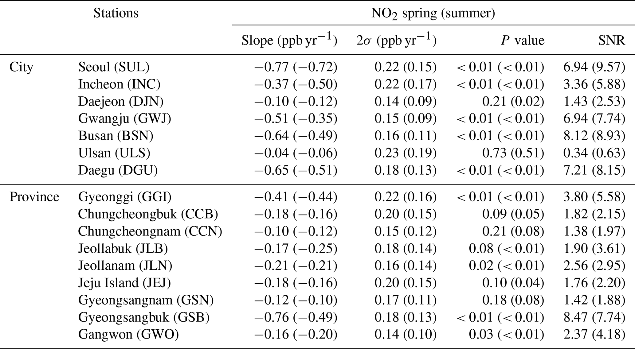
Table 4 The observed trends of CO concentrations in spring and summer from linear fits of the data covering 2001–2021. The data were acquired from the surface monitoring network (NIER, 2022). The unit of the slope and limit (2σ=2 standard deviations) is parts per billion per year (ppb yr⁻¹). SNR denotes the signal-to-noise ratio, defined as the ratio of the absolute value of the slope to standard deviation. For the use of P value and SNR, refer to Chang et al. (2021). Due to data limitations, the trend for the background sites could not be calculated.

Ozone increases in South Korea despite the reduction in the main precursors at a local scale can be attributed to the increase in the long-range transport of ozone or potentially the “VOC-limited” (or “NO_x-saturated”) local photochemical regime of South Korea. The VOC-limited regime is the condition in which NO_x (sum of NO and NO₂) concentration is high and VOC is a limiting factor to form ozone. In this case, VOC reduction would decrease ozone, while NO_x reduction would nonlinearly increase ozone. Since long-range transport from China is frequent during spring, it is useful to identify characteristics of ozone exceedance in spring separate from summer.

3.3 Changes detected during the COVID-19 pandemic (2020–2021) compared to 2002–2019

Nationwide social distancing protocol enforced by the South Korean government started on 25 February 2020 and lasted until 18 April 2022, although levels of protocol differed. During spring in 2020 (until 6 May 2020), facilities for public use (libraries, swimming pools, museums, and national parks) and religious, indoor sports, and entertainment facilities were forced to close, and people refrained from going out except for buying necessities, visiting a doctor, and commuting to and from work. From 6 May 2020, as the number of new confirmed COVID-19 cases remained relatively steady, the guidelines shifted from social distancing to distancing in daily life, with no restrictions on people going out. Because a cluster of new COVID-19 cases emerged in mid-August, social distancing protocol (since August 16 until early October) was again enforced by the government; people were strongly recommended to stay indoors. After 16 August 2020, there were well-defined government protocols as Level 1, 2, and 3: Level 1 was for no restrictions on private gatherings and daily life; Level 2 allowed for private gatherings of up to eight people and discouraged unnecessary and non-urgent travel; and Level 3 allowed private gatherings of up to three people, required remote work and online classes, and discouraged travel. Most days in spring and summer in 2021 fell in the period under the Level 2 protocol. In summary, most distinct changes in social-distancing protocols and traffic/mobile activities occurred between spring and summer in 2020 in South Korea (refer to Supplement 1 Figs. S14–S15).

3.3.1 Changes in ozone exceedances and local precursors during springtime

The frequency of springtime ozone exceedances increased from period P1 (2002–2010) to period P2 (2011–2019) across all observation sites in South Korea (Fig. 7). However, during the COVID-19 period (P3: 2020–2021), the frequency of exceedances significantly decreased at most sites. Notable reductions are observed in Daejeon, Daegu, Chungcheongbuk-do, Gyeongsangnam-do, Gyeongsangbuk-do, and Gangwon-do, as well as the background sites Gosung (Gangwon-do) and Ulleung Island. In Gosung, the percentage of ozone exceedances dropped from 30 % during P2 to 5 % during P3 in spring. Although Gosung is located close to the East Sea and is the region farthest from China within a similar latitude range, it is still susceptible to long-range-transported ozone due to its high elevation (see Supplement 1 Fig. 10 for the elevation map and diagram of a possible ozone transport path).

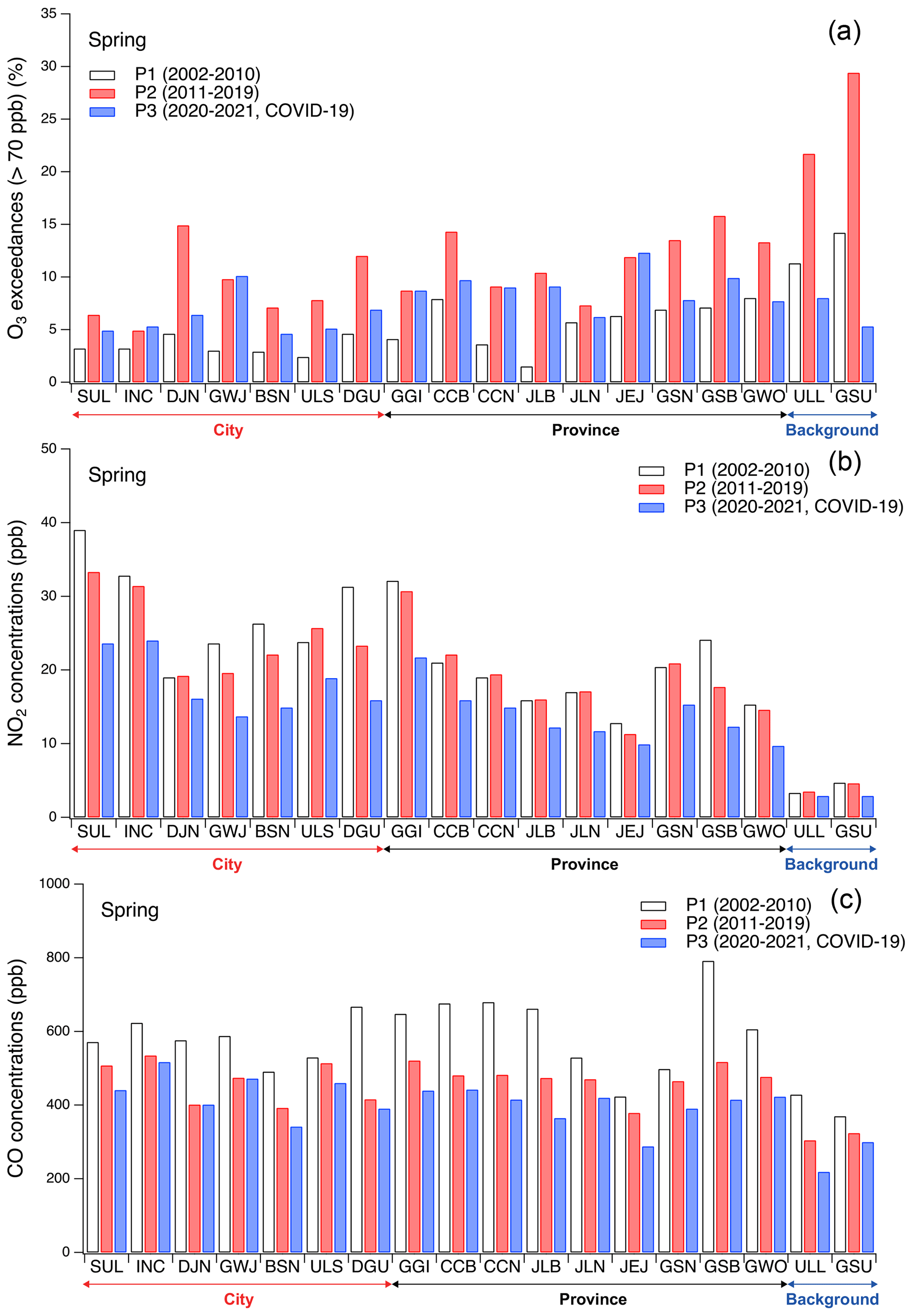
Figure 7 (a) O₃ exceedances (%), (b) NO₂, and (c) CO concentrations in South Korean cities, provinces, and background sites during spring for 2002–2010, 2011-2019, and 2020–2021 (COVID-19). The x axis denotes names of cities, provinces, and background sites. Cities – SUL (Seoul), INC (Incheon), DJN (Daejeon), GWJ (Gwangju), BSN (Busan), ULS (Ulsan), and DGU (Daegu). Provinces – GGI (Gyeonggi-do), CCB (Chungcheongbuk-do), CCN (Chungcheongnam-do), JLB (Jeollabuk-do), JLN (Jeollanam-do), JEJ (Jeju Island), GSN (Gyeongsangnam-do), GSB (Gyeongsangbuk-do), and GWO (Gangwon-do). Background sites – ULL (Ulleung Island) and GSU (Gosung, Gangwon-do).

Across all sites, the concentration of NO₂ shows little change from P1 to P2, with an average decrease of 5 %. However, during the COVID-19 period (P2 to P3), there was an average reduction of 25 % in NO₂ concentrations. CO concentrations also experienced a decrease of 22 % from P1 to P2 and a further decrease of 14 % from P2 to P3. However, the reductions in CO are relatively minor compared to the changes in NO₂ observed during the COVID-19 period. The decrease in ozone exceedances during COVID-19 may be associated with the reductions in NO₂ concentrations during this time.

A notable finding is the significant reduction in ozone levels at the background sites, such as Gosung and Ulleung Island, between P2 and P3. This suggests a cleaner background influenced by changes in emissions from sources in Asia and long-range transport. It is important to note that there were no significant changes in NO₂ and CO concentrations observed at the background sites from P2 to P3. There are several studies reporting the increase in near-surface ozone after COVID lockdowns in the urban areas (e.g., Shi and Brasseur, 2020) because of the expected nonlinear relationship between ozone and NO_x in the highly polluted regions. However, there are also studies reporting reductions of ozone concentrations from 1 to 8 km altitude in the northern extratropics during COVID (Steinbrecht et al., 2021). Parrish et al. (2020) reported zonal similarity of tropospheric ozone changes at northern midlatitudes. Therefore, ozone reductions from P2 to P3 across the sites in South Korea may be associated with decreased background ozone at northern midlatitudes to some extent. On top of this, local and regional emission changes during COVID may also play a role in reducing ozone exceedances in South Korea in this season.

3.3.2 Changes in ozone exceedances and local precursors during summertime

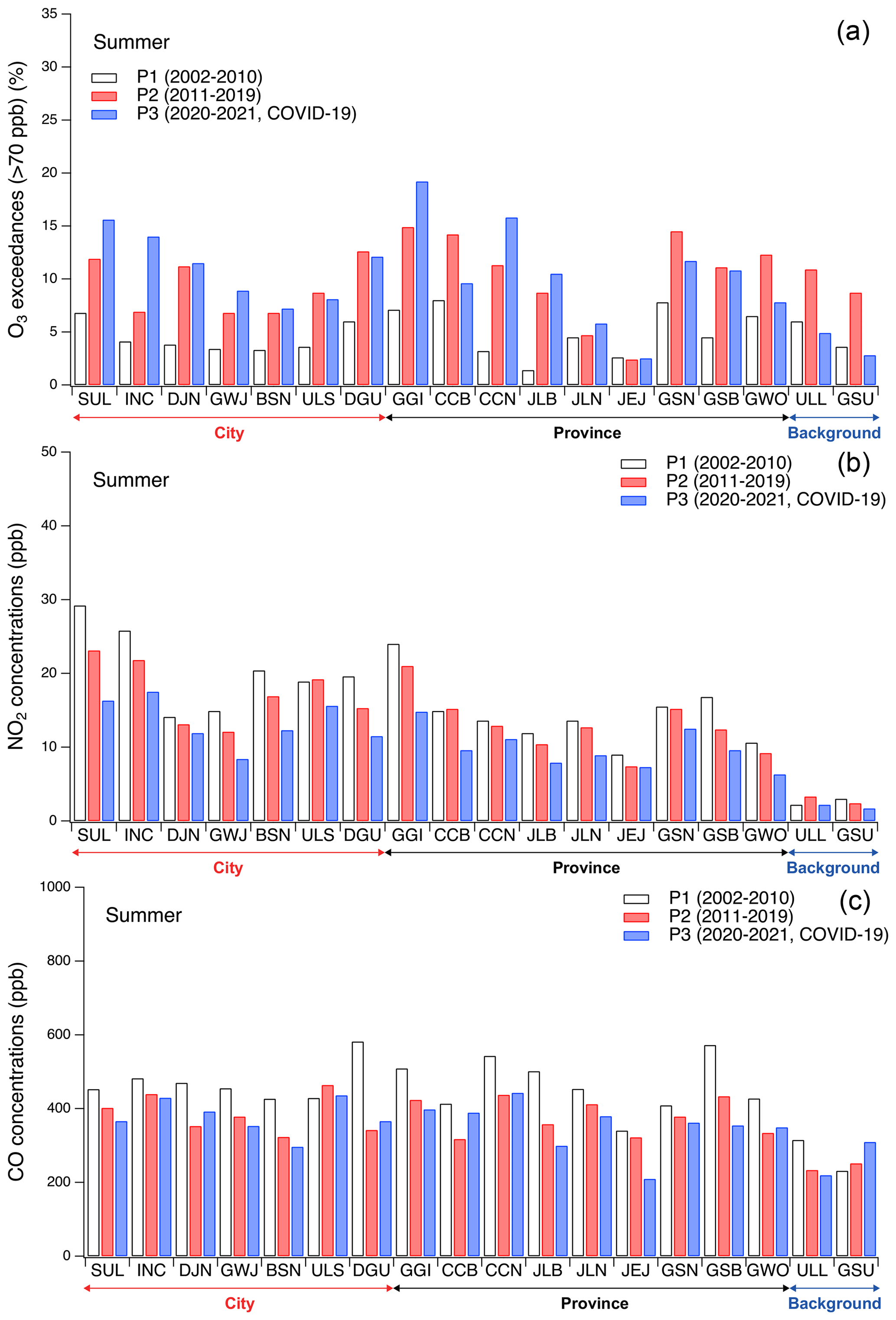
During summer, ozone exceedance frequencies also increase from P1 to P2 for all sites: Chungcheongnam-do has the largest increase from 3.2 % to 11.3 %, and Gyeonggi-do, Daejeon, Jeollabuk-do, Gyeongsangnam-do, and Gyeongsangbuk-do have similar increases (Fig. 8). The ozone exceedances in the background sites Gosung and Ulleung Island also increase in this period. NO₂ and CO concentrations decreased marginally from P1 to P2. During COVID-19, the ozone exceedance frequencies in summer increase in Seoul, Incheon, Gyeonggi-do, and Chungcheongnam-do; substantially decrease in Gangwon-do and the background sites; and do not show changes from P2 for the rest of sites. Because NO₂ concentrations decrease from P2 to P3 for Seoul, Incheon, Gyeonggi-do, and Chungcheongnam-do, contrasting with increases of ozone exceedance, the chemical regime for these regions during summer is likely to be VOC-limited (NO_x-saturated) as mentioned above and as in previous studies (e.g., Kim et al., 2020). Ozone exceedance substantially decreases in the background sites from P2 to P3 during summer, indicating cleaner air at a large scale, as shown in Steinbrecht et al. (2021).

Figure 8 The same as Fig. 7 except for summer.

3.3.3 Changes in precursor concentrations at a regional scale during spring and summer: TROPOMI tropospheric NO₂ columns

Figure 9 presents the spatial distributions of NASA TROPOMI tropospheric NO₂ columns (Lamsal et al., 2022) in spring (MAM) and summer (JJA) across East Asia, along with their changes from 2019 to 2020 and from 2019 to 2021. The plot illustrates significant reductions in NO₂ columns during the spring of COVID-19 in most areas of China, South Korea, and the surrounding seas. Changes in traffic activities in the Seoul Metropolitan Area were also detected between 2019 and 2020 (refer to Supplement 1 Figs. S14 and S15). The number of cars counted at the highway tolls in this region decreased by 6 % in March, April, and May in 2020 compared to 2019, but this trend was reversed in June (Supplement 1 Fig. S14). Furthermore, observed concentrations of NO₂, SO₂, CO, PM₁₀, and PM_2.5 during the spring of 2020 showed reduction of 15 %–30 % (Supplement 1 Fig. S15). Changes in traffic counts in the Seoul Metropolitan Area between 2019 and 2021 were small (Supplement 1 Figs. S14 and S15). But observed concentrations of NO₂, SO₂, CO, PM₁₀, and PM_2.5 were also reduced during spring in 2021 compared to 2019 by 10 %–30 % except for PM₁₀ that was enhanced due to Asian dust events in spring 2021 (Supplement 1 Fig. S15).

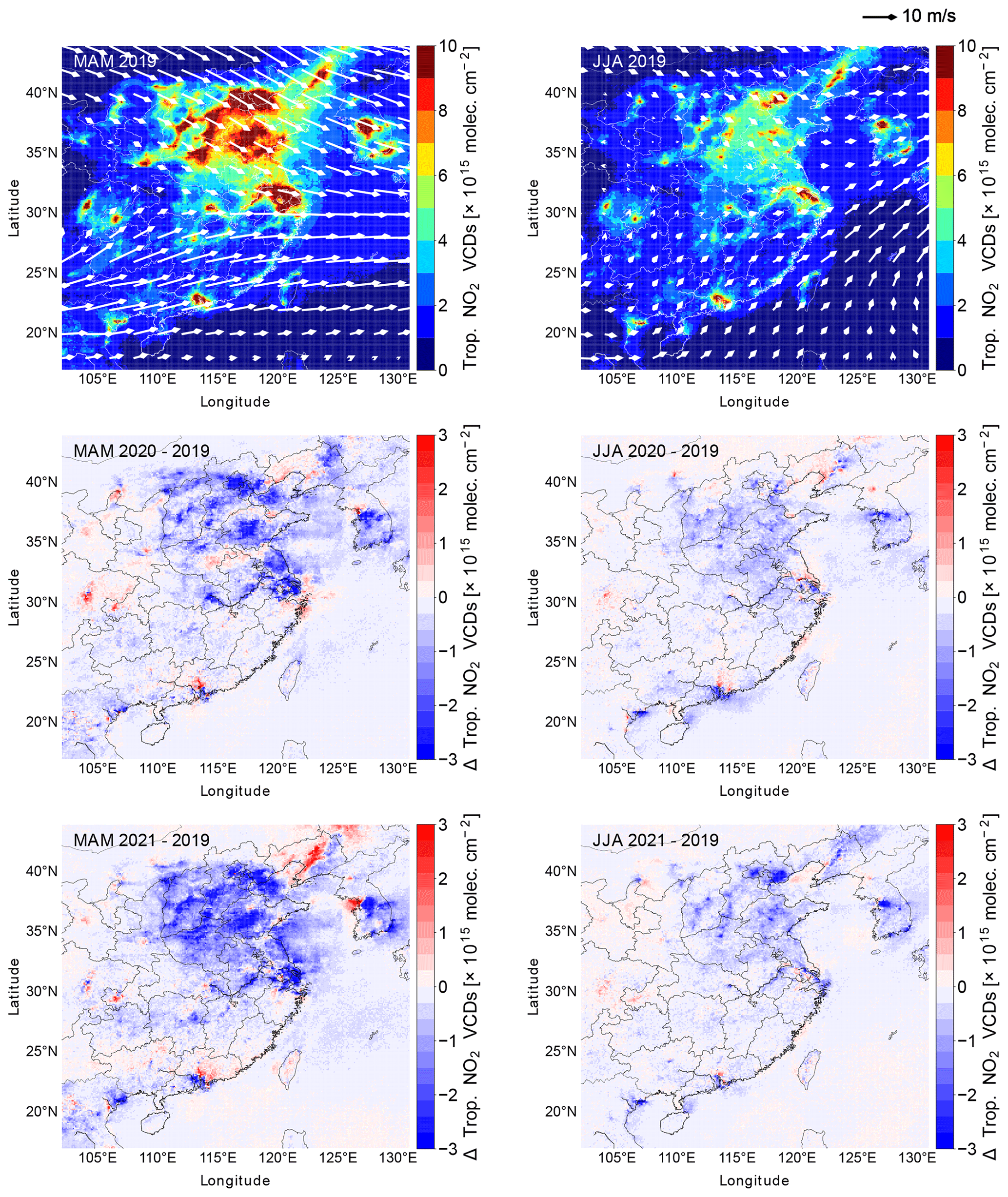
Figure 9 Differences in TROPOMI tropospheric NO₂ columns between 2019 and 2020 or between 2019 and 2021 (difference = NO_{2 2020 or 2021}–NO_2 2019). The unit is molecules per square centimeter. Wind vectors at 700 hPa from ERA-5 are shown for MAM and JJA, respectively. Here, ERA-5 denotes the fifth-generation European Centre for Medium-Range Weather Forecasts reanalysis (https://doi.org/10.24381/cds.6860a573).

As depicted in Fig. 9, TROPOMI tropospheric NO₂ columns also decreased during the summer in the same region, although in fewer locations and to a lesser extent compared to the spring, during the COVID-19 period. The observed NO₂, SO₂, CO, PM₁₀, and PM_2.5 concentrations in the Seoul Metropolitan Area were also reduced during summer in 2020 or 2021 compared to 2019 by 2 %–20 %. Surface NO₂ concentrations reduced by ∼ 10 % during summer, which is smaller than the reductions during spring (∼ 20 %; see Supplement 1 Figs. S14 and S15). Overall, the reductions in 2020/2021 from 2019 during summer are smaller than those during spring at the surface in the Seoul Metropolitan Area, similar to the seasonal changes detected from space.

The substantial decrease in NO₂ in China during spring, observed by satellite, is likely to contribute to significant reductions in ozone levels in South Korea due to long-range transport. Additionally, local reductions in NO_x emissions in South Korea can lead to ozone decreases if the reductions are significant enough, especially in the VOC-limited chemical regime prevalent in this area. However, further investigation is required to understand the detailed source–receptor mechanism of ozone and its precursors in each season, which warrants long-term air quality model simulations in future studies. The next section of this study discusses the sensitivity of ozone concentrations in Seoul and Gangwon-do to various emission scenarios in China and South Korea, albeit within a limited time period.

3.4 Impacts of changes in East Asian emissions on surface/boundary- layer ozone in South Korea: a modeling analysis

3.4.1 Changes in surface/boundary-layer ozone due to emission reductions: East Asian region

In this section, we will discuss WRF-Chem model simulations conducted during the KORUS-AQ 2016 field campaign (primarily in May; refer to Crawford et al., 2021, for detailed information) to gain insights into the impacts of emission changes on ozone concentrations in East Asia, including South Korea. We have extensively evaluated our model results with the airborne and surface observations acquired during the KORUS-AQ campaign and the routine surface monitors in China and South Korea. The model decently simulated boundary-layer ozone over South Korea (3 % difference) for the cases that were strongly influenced by long-range transport. For local-emission-dominating cases, the model underestimated boundary-layer ozone over South Korea by 20 %. The results are summarized in Supplement 1 (Table S3 and Fig. S8) and Kim et al. (2023). This study considers two extreme cases: the No China case, where all anthropogenic emissions in China are removed, and the No Seoul case, where all anthropogenic emissions in Seoul are removed. Additionally, several other scenarios are examined, including a 50 % reduction in Chinese NO_x emissions only, a 50 % reduction in Chinese VOC emissions only, a 50 % reduction in both Chinese NO_x and VOC emissions, and a 75 % reduction in Chinese NO_x emissions only.

Our study reveals both increases and decreases in ozone concentrations due to emission changes resembling those during the COVID-19 period. Specifically, near-surface ozone concentrations in polluted regions increase, while ozone concentrations in the elevated layer show reductions (refer to Figs. 10 and 11). A novel finding is the decrease in downwind ozone, from the near surface to the upper layer, resulting from reductions in NO_x $/$ VOC emissions in upwind pollution hotspots (refer to Figs. 10 and 11 for several sensitivity runs). For instance, a 50 %–75 % reduction in Chinese NO_x emissions leads to decreased ozone concentrations in Korea, surrounding seas, and the Pacific Ocean, from the surface to the upper layers. However, near-surface ozone in northeast China increases due to these emission changes.

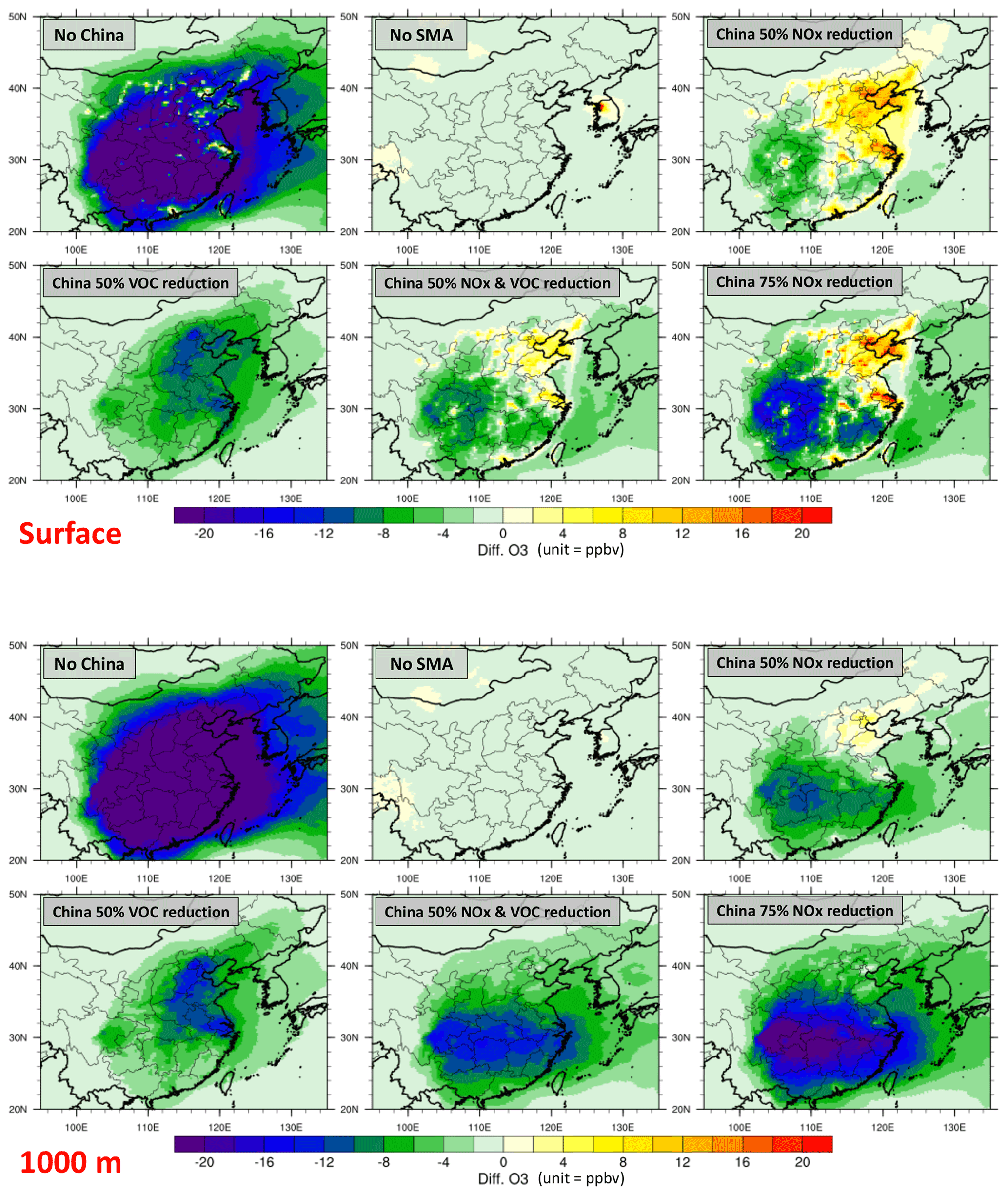
Figure 10 Differences in the WRF-Chem simulated ozone concentrations (ΔO₃= O₃_emission reduction case-O₃_control case) at (top) surface and (bottom) 1000 m above ground level. Green to blue colors (yellow to red colors) denote reduced (increased) ozone concentration due to the emission changes. All model simulation results are utilized.

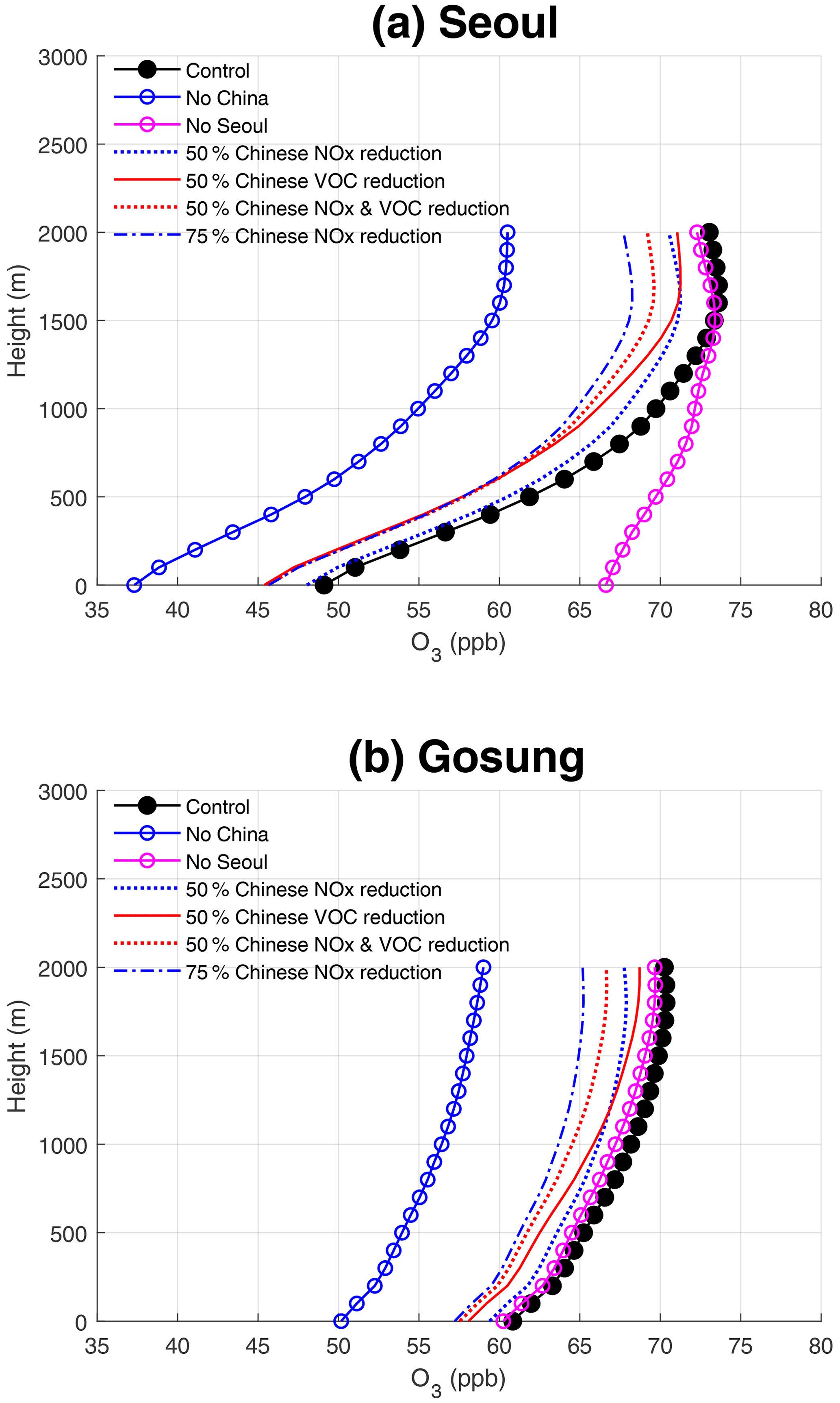
Figure 11 Vertical profiles of ozone from the WRF-Chem model simulations based on various emission scenarios: (a) Seoul and (b) Gosung, Gangwon-do. The model results from 10:00 to 20:00 LT are averaged.

Reductions in Chinese VOC emissions result in decreased ozone concentrations from the surface to the upper layer and from hotspots to downwind areas. Our study suggests potential changes in photochemical regimes with altitude over pollution hotspots, indicating NO_x-saturated conditions near the surface and NO_x-limited conditions in the elevated layer. Thus, the combined effects of vertical and horizontal ozone transport, as well as local production dependent on altitude, would determine the ultimate changes in ozone concentrations at specific locations and altitudes. It is important to note that the accuracy of VOC emission estimates also influences the assessment, but this aspect is highly uncertain and requires further study.

3.4.2 Vertical sensitivity of ozone changes in South Korea to East Asian emission reductions

Figure 11 presents the vertical profiles of simulated ozone concentrations for different emission scenarios. In Seoul, the 50 % reduction in Chinese NO_x emissions only slightly decreases ozone concentrations near the surface but decreases them above 500 m a.g.l. (above ground level) to a larger extent. The 50 % reduction in Chinese VOC emissions causes a decrease in ozone concentrations from the surface to 2000 m a.g.l. In the elevated layer (> 1500 m a.g.l.) in Seoul, the reduction in Chinese NO_x emissions leads to a greater decrease in ozone concentrations compared to the reduction in Chinese VOC emissions. The scenario with a 50 % reduction in both Chinese NO_x and VOC emissions efficiently decreases ozone concentrations from the surface to 2000 m a.g.l., particularly above 1000 m a.g.l. The scenario with a 75 % reduction in NO_x emissions decreases ozone concentrations near the surface similarly to the scenarios with a 50 % reduction in NO_x and VOC emissions, but it causes the largest ozone reductions above 1000 m a.g.l., except for the No China emission scenario. The No China emission scenario results in ozone concentrations 10–15 ppb lower than the control case at all altitudes. On the other hand, the No Seoul emission scenario leads to ozone concentrations about 20 ppb higher than the control case near the surface, partly due to significantly reduced ozone depletion reactions with NO. The sensitivity test results for Seoul and Gosung, Gangwon-do, are similar, except that all emission scenarios (including No Seoul and 50 % reduction in Chinese NO_x scenarios) cause a decrease in ozone concentrations in Gangwon-do. Both NO_x and VOC emission reductions in China contribute to cleaner air in Gangwon-do, with the largest cleaning effect observed above 500 m a.g.l. This may explain the sharp decline in ozone exceedances observed in Gosung, located at an elevation of approximately 600 m a.g.l., during the COVID-19 pandemic (Fig. 7). Refer to Supplement 1 (Table S6 and Fig. S10) about altitudes of monitoring sites in Gangwon-do including Gosung. The sensitivity runs clearly demonstrate the long-range transport of Chinese ozone or the influence of Chinese emissions on the eastern part of the Korean Peninsula, such as Gangwon-do, from May to the beginning of June 2016. Both reductions in Chinese VOC emissions and NO_x emissions contribute to improving ozone pollution in the boundary layer (1–3 km) in South Korea.

3.4.3 Comparisons with recent modeling research

Lee and Park (2022) investigated seasonal differences in ozone utilizing a chemical transport model. They reported the April mean ozone concentration of 39.3 ppb, which is slightly higher than the July counterpart (38.3 ppb) from their model simulations for the year 2016 and the selected surface monitor sites for four main regions (Seoul, Chungcheongbuk-do, Gwangju, and Busan). Our study summarizes the differences between spring (March, April, May) and summer (June, July, August) for 21 years including 192 monitoring sites covering the whole of South Korea, focusing on the analysis of long-term surface ozone observations. On overage, the observed spring mean ozone is 34.3 ppb, and the summer mean ozone is 29.0 ppb over South Korea in our study. Lee and Park (2022) indicated that ozone air quality in South Korea is determined mainly by year-round regional background contributions (peak in spring). With some differences in details, the results from the two studies are qualitatively similar arguing high springtime background ozone value. One unique aspect of our modeling study is demonstrations of the impact of emissions in Seoul on Gangwon-do, causing a slight ozone decrease in Gangwon-do with no emissions from Seoul from the surface to 2 km in May 2016. Our study highlights the diverse impacts of surface emission changes (over China or Seoul) on downwind ozone at different altitudes (Fig. 11).

Colombi et al. (2023) performed an analysis of the effect of precursor changes on observed surface ozone increases in South Korea. The main difference between Colombi et al. (2023) and our study is the period of the study and whether it focuses on the surface ozone or vertical sensitivity explaining ozone variability at different locations in South Korea. Our study investigated surface ozone and ozone at various altitudes to consider the transport within and above the boundary layer between China and South Korea. Colombi et al. (2023) analyzed the surface ozone and NO₂ concentrations, mainly over the Seoul Metropolitan Area from 2015 to 2019. The increase in ozone was mostly attributed to decrease in NO₂ for the studied period.

Both Lee and Park (2022) and Colombi et al. (2023) indicated high background ozone concentration external to East Asia (or South Korea), suggesting difficulty of achieving ozone standards. Our study agrees on this point. Probably one different message is that reducing emissions of NO_x and VOC here and there all together have positive impacts on reducing ozone downwind. For example, emission reductions associated with the COVID-19 would lead to a decrease in ozone at most sites over South Korea in spring. However, our study also indicates that the ozone exceedances notably increased in the Seoul Metropolitan Area (SMA) and Chungcheongnam-do (where large mobile, industrial, and power plant emission sources are located) during the summer of the COVID-19 pandemic.

4 Conclusions

We conducted a study on the spatiotemporal variability of surface ozone in seven cities, nine provinces, and two background sites in South Korea from 2001 to 2021. The fourth-highest maximum daily 8 h average (MDA8) ozone concentrations showed an increasing trend in all cities, most provinces, and background sites during this period (or 2001 to 2019), with a yearly increase of 1–2 ppb. After 2010, these concentrations reached approximately 70 ppb or higher. If the US EPA National Ambient Air Quality Standards were applied, most of the monitoring sites in South Korea would have been considered nonattainment areas for the past decade.

Ozone exceedances in this study were defined as the ratio of data with concentrations exceeding 70 ppb to the total data, which aligns with the US EPA standard. In Seoul, Incheon, and Gyeonggi-do, ozone exceedances were more frequent in summer than in spring. However, the opposite trend was observed in Daejeon, Gwangju, Jeollanam-do, Gyeongsangbuk-do, Gangwon-do, Jeju Island, and the background sites Gosung and Ulleung Island. In other areas, the frequencies of exceedances were similar between spring and summer. The majority of ozone exceedances occurred between 16:00–19:00 LT (16:00–19:00). Interestingly, exceedances also occurred frequently at night in background sites such as Gosung and Ulleung Island, indicating a strong influence of long-range transport on surface ozone levels in these locations.

Ozone exceedances increased from period P1 (2002–2010) to period P2 (2011–2019) across all observation sites in South Korea during spring and summer. Overall, NO₂ concentrations showed declining trends from 2001 to 2021, but significant and relatively large decreases were only evident after the mid-2010s. NO₂ concentrations for P1 and P2 were similar, and an increase in CO $/$ VOC concentrations between the two periods was not detected or reported. Therefore, it is not clear what drove the increase in ozone exceedances over South Korea from P1 to P2. The observed increase in ozone exceedances from P1 to P2 in South Korea may be partially attributed to the rise in anthropogenic emissions originating from China. More modeling experiments covering the P1 to P2 period would help identify the main factors behind the ozone increases. It is important to investigate not only changes in anthropogenic emissions but also the impact of climate change on ozone variations during this period. We observed significant reductions in ozone exceedances across almost all monitoring sites in South Korea during the spring of the COVID-19 pandemic (period P3, 2020–2021), which was attributed to decreased anthropogenic activities and subsequent lower emissions in both China and South Korea. It should be noted that ozone exceedances substantially increased in the SMA and Chungcheongnam-do during the summer of the COVID-19 pandemic. We conducted sensitivity tests using a regional chemical model to investigate the impact of emission changes on ozone pollution in South Korea for a limited period in spring. The results suggest that reductions in Chinese NO_x emissions as well as VOC emissions can contribute to the improvement of ozone pollution in South Korea. These findings provide valuable insights for future efforts to address ozone pollution in South Korea and emphasize the need for further research to project air quality and prioritize actions for the next decade or so.

In the future, employing multi-decadal mathematical modeling on a local to global scale in both hindcast and forecast modes would be beneficial for better understanding ozone trends in South Korea. Additionally, reliable VOC observations and conducting intensive field campaigns, similar to the KORUS-AQ 2016, would provide crucial information to unravel the complexities of ozone chemistry in this region and facilitate the careful monitoring of changes in atmospheric composition relevant to ozone. Monitoring ozone within the boundary layer and at higher altitudes is crucial for enhancing our understanding of ozone trends in South Korea. A network of ozonesondes at multiple sites with the capability of weekly launches would be a valuable complement to a large field campaign.