Sub-cloud rain evaporation in the North Atlantic winter trade winds derived by pairing isotopic data with a bin-resolved microphysical model

Sub-cloud rain evaporation in the trade wind region significantly influences the boundary layer mass and energy budgets. Parameterizing it is, however, difficult due to the sparsity of well-resolved rain observations and the challenges of sampling short-lived marine cumulus clouds. In this study, sub-cloud rain evaporation is analyzed using a steady-state, one-dimensional model that simulates changes in drop sizes, relative humidity, and rain isotopic composition. The model is initialized with relative humidity, raindrop size distributions, and water vapor isotope ratios (e.g., δD_v, ${{\mathit{\delta }}^{\mathrm{18}}\mathrm{O}}_{\mathrm{v}}$) sampled by the NOAA P3 aircraft during the Atlantic Tradewind Ocean–Atmosphere Mesoscale Interaction Campaign (ATOMIC), which was part of the larger EUREC⁴A (ElUcidating the RolE of Clouds–Circulation Coupling in ClimAte) field program. The modeled surface precipitation isotope ratios closely match the observations from EUREC⁴A ground-based and ship-based platforms, lending credibility to our model. The model suggests that 63 % of the rain mass evaporates in the sub-cloud layer across 22 P3 cases. The vertical distribution of the evaporated rain flux is top heavy for a narrow (σ) raindrop size distribution (RSD) centered over a small geometric mean diameter (D_g) at the cloud base. A top-heavy profile has a higher rain-evaporated fraction (REF) and larger changes in the rain deuterium excess ($d=\mathit{\delta }D-\mathrm{8}\times {\mathit{\delta }}^{\mathrm{18}}\mathrm{O}$) between the cloud base and the surface than a bottom-heavy profile, which results from a wider RSD with larger D_g. The modeled REF and change in d are also more strongly influenced by cloud base D_g and σ rather than the concentration of raindrops. The model results are accurate as long as the variations in the relative humidity conditions are accounted for. Relative humidity alone, however, is a poor indicator of sub-cloud rain evaporation. Overall, our analysis indicates the intricate dependence of sub-cloud rain evaporation on both thermodynamic and microphysical processes in the trade wind region.

1 Introduction

Shallow precipitation is a sporadic but energetically significant feature of marine cumulus clouds in the trade wind tropical ocean basins (Byers and Hall, 1955; Nicholls and Leighton, 1986; Paluch and Lenschow, 1991; Short and Nakamura, 2000; Jensen et al., 2000; Stevens, 2005). Rain rates on the scale of 1 mm d⁻¹, commonly associated with shallow cumulus precipitation, are capable of producing roughly 28 Wm⁻² of latent heat flux through rain evaporation in the sub-cloud layer (Fig. 1), which is comparable to the radiative and surface fluxes computed using mixed-layer models (e.g., Caldwell et al., 2005) and within stratocumulus-to-cumulus transition regions (e.g., Kalmus et al., 2014).

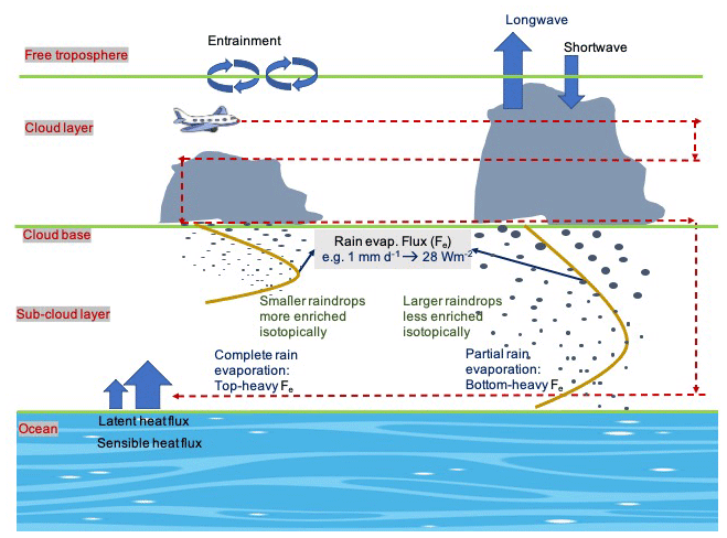
Figure 1 Schematic showing rain from a cumulus-topped boundary layer, with the latent and sensible heat fluxes near the surface. The longwave and shortwave fluxes and free-tropospheric entrainment mixing are shown at the cloud top. Rain can evaporate completely or partially as it falls toward the surface. This could lead to differences in the vertical profiles of the rain evaporation fluxes depicted by the solid vertical curves. Complete evaporation of rain could cause the maximum rain evaporation flux close to the cloud base (top heavy) compared to partial evaporation, which could bring the maxima closer to the surface (bottom heavy). A 1 mm d⁻¹ rain rate can potentially produce 28 Wm⁻² of a rain evaporation flux. The aircraft measurements are made at horizontal above-cloud, in-cloud, cloud base, and near-surface legs, as shown by airplane cartoon and the dashed red line trajectories.

Such large fluxes, even if localized, may influence the vertical moisture and energy distribution and affect the boundary layer stability (e.g., Srivastava, 1985; Paluch and Lenschow, 1991). The evaporatively cooled air mass also facilitates downdrafts below the cloud base, which initiate or strengthen cold pool formations (Srivastava, 1985; Jensen et al., 2000; Seifert, 2008; Zuidema et al., 2012; de Szoeke et al., 2017). The downdraft can further feed its cool and moist air into large-scale circulations, leading to moisture recycling (Stevens, 2005; Worden et al., 2007). A schematic of these processes is shown in Fig. 1.

The rain evaporation efficiency, or the fraction of rain evaporated in the sub-cloud layer, impacts the amount of rain that reaches the surface. Depending on the fraction of rain reaching the surface and the sub-cloud moisture circulation, clouds could either remain intact or break up, thus affecting the local albedo (Paluch and Lenschow, 1991; Sandu and Stevens, 2011; Yamaguchi et al., 2017; O et al., 2018; Sarkar et al., 2020). Overall, accurate rain evaporation estimates in shallow cumulus regions are needed to better predict surface rain estimates in weather and climate models and understand the shallow rain life cycle.

Past field campaigns have sampled precipitation from shallow cloud systems. For example, the Atlantic Stratocumulus Transition Experiment (ASTEX; Bretherton and Pincus, 1995) conducted over the east-central Atlantic Ocean in June 1992 sampled the cloud systems, with drizzle evaporating into the sub-cloud layer beneath overlying stratocumulus clouds. Similarly, the Rain in Cumulus over the Ocean (RICO; Geoffroy et al., 2014; Snodgrass et al., 2009) campaign was conducted off the Caribbean islands of Antigua and Barbuda over the Atlantic Ocean in 2012–2013, where cumulus rain was sampled. Furthermore, the Cloud System Evolution in the Trades (CSET; Albrecht et al., 2019; Mohrmann et al., 2019; Sarkar et al., 2020) was conducted over the Pacific Ocean between California and Hawaii in July–August 2015 to sample stratocumulus and cumulus rain events. These campaigns support the idea that shallow precipitation and sub-cloud evaporation is important for the local energy budget. However, a more dedicated study is needed to characterize the shallow cloud rain evaporation as a function of the local thermodynamic and microphysical conditions.

Questions also remain about the rain evaporation flux (F_e) variability in different cloud conditions and its sensitivity to boundary layer microphysical and thermodynamic characteristics. How is the vertical structure of F_e linked to microphysical and thermodynamic processes? Could F_e reinforce or weaken sub-cloud stability at local scales? These questions are inherent to our understanding of shallow rain processes and constraining F_e accurately.

A major challenge when observationally constraining rain evaporation is sampling rain in and below cumulus clouds, due mainly to their temporal and spatial variability and the limitations in the existing rain retrieval methods. The airborne millimeter wavelength radar used during field campaigns provides a wide and homogeneous array of cloud and precipitation samples in terms of radar moments. However, accurate microphysical retrievals from the radar moments are difficult due to Mie scattering and atmospheric and liquid attenuations (Fairall et al., 2018; Schwartz et al., 2019; Sarkar et al., 2021). Rain observations from satellites, although they provide a large array of datasets, are often limited in their sensing accuracy of shallow rain. This is due to factors like high atmospheric attenuation and surface radar reflections (e.g., Kalmus et al., 2014).

In comparison, in situ cloud and rain probes, although limited in their sampling volume when compared to radar, provide well-resolved, direct, and accurate microphysical raindrop size distributions (RSDs). In situ measurements also provide stable isotope ratios of hydrogen and oxygen in water vapor, which can be used to independently assess rain evaporation. This is because as rain evaporates into the unsaturated sub-cloud layer, the isotopically light water transitions to the vapor phase more efficiently, causing the drops to become increasingly heavy (Salamalikis et al., 2016; Graf et al., 2019).

This study makes a novel attempt to characterize rain evaporation, its vertical structure, and its dependence on microphysical (i.e., raindrop concentration, size, and distribution width) and thermodynamic (i.e., surface relative humidity) features using a one-dimensional, steady-state evaporation model initialized by in situ field observations of both RSD and water vapor isotope ratios. The in situ samples were measured by the NOAA WP-3D Orion (P3) aircraft during the Atlantic Tradewind Ocean–Atmosphere Mesoscale Interaction Campaign (ATOMIC), which was a component of the international field campaign known as EUREC⁴A (ElUcidating the RolE of Clouds–Circulation Coupling in ClimAte). For the first time, the isotopic enrichment of rain is modeled using RSDs measured in the field and evaluated using surface-based isotopic rain observations.

First, the rain observations are characterized at the cloud base in terms of microphysical and thermodynamic conditions. Second, the vertical distribution of the sub-cloud-modeled rainwater content (RWC) and rain evaporation fluxes (F_e) are discussed in terms of their microphysical and thermodynamic sensitivities. Last, the modeled isotope ratios at the surface are also compared with the surface isotope ratio observations in the P3 vicinity to validate the accuracy of the model. We expect results from this work to pave the way toward a better representation of shallow rain evaporation in climate models and to serve as a model for comparing rain evaporation processes in a wide range of convection.

2 Data and methodology

2.1 ATOMIC and EUREC⁴A campaign and datasets

The ATOMIC field campaign was conducted in the North Atlantic trade wind region, roughly between 10–15^∘ N and 51–60^∘ W, to study mesoscale circulations in the atmosphere and ocean (Pincus et al., 2021). ATOMIC was the NOAA-sponsored component of the larger, international EUREC⁴A field campaign, which took place in January–February 2020 near Barbados (Stevens et al., 2021). Both the NOAA P3 aircraft and the NOAA R/V Ronald H. Brown (hereafter Ron Brown) were deployed as part of ATOMIC. Other platforms, such as the R/V Meteor and Barbados Cloud Observatory (BCO), discussed in this paper were part of the larger EUREC⁴A effort.

The P3, integrated with radar, in situ instruments, and dropsondes, was flown through cloud and rain transects to collect thermodynamic and microphysical boundary layer observations and facilitate investigations of aerosol–cloud–precipitation interactions. An example of the trajectory of the P3 is shown in Fig. 2 for 9 February, where a series of stacked 10 min horizontal legs were flown to sample the boundary layer extensively. The horizontal legs were flown at 150, 500, and 700 m and 2, and 3 km between 54 and 56^∘ W. During most flights, a level circle was also conducted at 7.5 km altitude, and seven to eight dropsondes were released to obtain high-resolution thermodynamic observations reaching the surface. The surface relative humidity, which is integral to the rain evaporation model used in this paper, is obtained at ≈10 m altitude. Its values for 9 February are noted at the dropsonde locations in Fig. 2b.

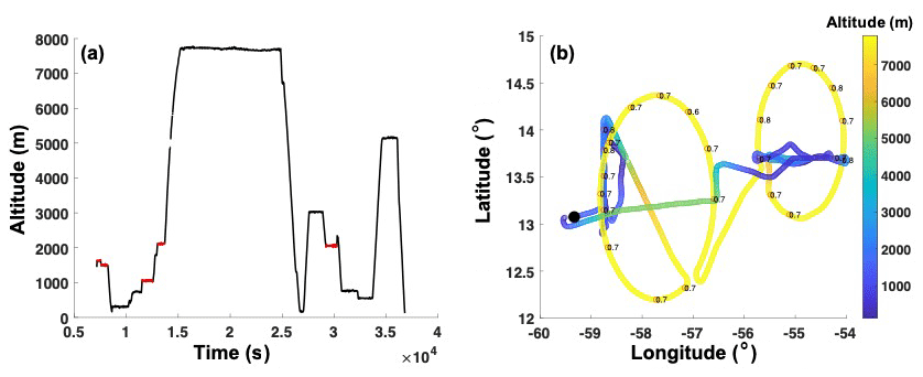
Figure 2 P3 trajectory on 9 February (a) in time–altitude axes and (b) in longitude–latitude axes, with contour colors showing the altitude (in meters) of the P3. The red lines in panel (a) denote the legs with mean rain rates greater than 0.01 mm d⁻¹ that are selected for this study. Numbers in panel (b) denote the surface relative humidity in a fraction of 1 over the dropsonde locations.

This paper characterizes the rain structure during ATOMIC using the Cloud Imaging Probe (CIP) and Precipitation Imaging Probe (PIP) instruments on board the P3, which sampled the raindrop size distributions in situ. The CIP samples cloud drops and raindrops across diameters of 25 µm–1.6 mm, while the PIP samples across 100 µm–6.2 mm (Pincus et al., 2021; Leandro and Chuang, 2021). The CIP and PIP observations are stitched together to obtain 1 Hz raindrop size distributions for diameters spanning 100 µm–6 mm (total 23 bins). Bin sizes smaller than 100 µm and bigger than 6 mm are not reliable and are not used in the current analysis. Drops across 400–1800 µm, 1.8–5 mm, and 5–6 mm drop sizes are binned at 200 µm, 400 µm, and 1 mm resolutions, respectively.

This paper is based on the latter part of the ATOMIC campaign, when the CIP and PIP instruments were properly functioning and mean rain rates greater than 0.01 mm d⁻¹ were observed during 22 10 min in-cloud horizontal legs on 4, 5, 9, and 10 February. The in-cloud RSD is assumed to accurately represent cloud base RSD. The rain rates (in mm d⁻¹) are calculated from the observed RSD, using $R=\mathrm{6}\mathit{\pi }\times {\mathrm{10}}^{-\mathrm{7}}{\sum }_{i=\mathrm{1}}^{\mathrm{23}}N\left(D_i\right)v_i{D}_i^{\mathrm{3}}$, where N (m⁻³) is the raindrop concentration for the drop diameter D_i (mm), v_i (m s⁻¹) is the terminal velocity associated with D_i, and i is the index of the RSD bin. The rain rates for each 10 min leg are averaged and noted in the legend of Fig. 3. Even though the probe instruments were working on 31 January and 11 February, the mean rain rates from those days were below 0.01 mm d⁻¹ during all of the 10 min in-cloud horizontal legs and are therefore not included in this study.

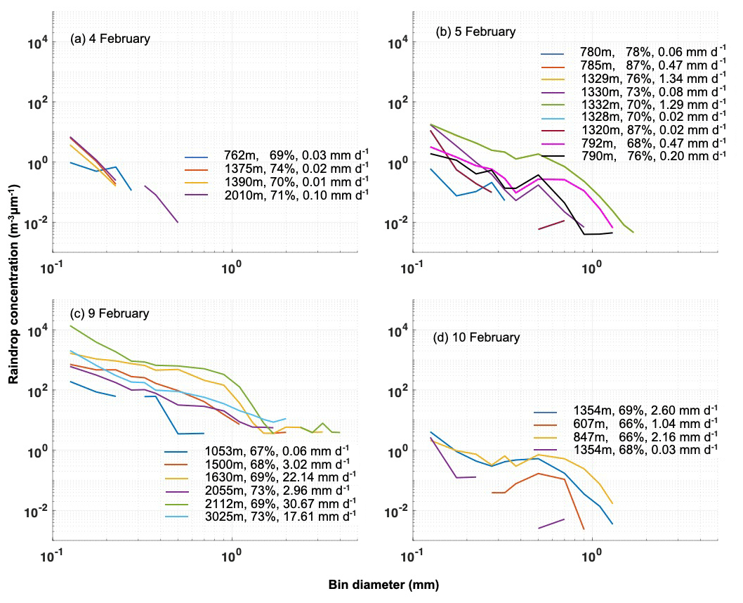
Figure 3 Raindrop size distribution is shown for 10 min horizontal legs on (a) 4, (b) 5, (c) 9, and (d) 10 February. The legend shows the altitude of the horizontal legs, dropsonde-derived surface relative humidity, and leg mean rain rates.

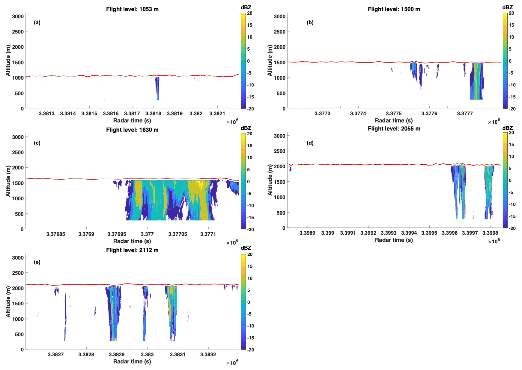
Figure 4 The 94 GHz radar reflectivity (in dBZ) on board the P3 on 9 February pointing downwards for all the six horizontal level legs shown in Fig. 2. The red line is the flight trajectory, and the contour shade represents the radar reflectivity.

To model the isotopic evolution of the RSDs, 1 Hz water vapor mixing ratio and water vapor isotope ratios for hydrogen and oxygen (δD_v and ${{\mathit{\delta }}^{\mathrm{18}}\mathrm{O}}_{\mathrm{v}}$, respectively) were obtained from the Picarro L2130-i water vapor isotope analyzer flown during ATOMIC (Bailey et al., 2023). When airborne, the analyzer drew in ambient air through a 0.25 in. (6.35 mm) backward-facing tube, which ensured the selective sampling of water vapor as opposed to liquid water (Pincus et al., 2021). δD_v and ${{\mathit{\delta }}^{\mathrm{18}}\mathrm{O}}_{\mathrm{v}}$ represent the ratios $D/H$ and ${}^{\mathrm{18}}\mathrm{O}{/}^{\mathrm{16}}\mathrm{O}$, respectively, normalized to VSMOW (Vienna Standard Mean Ocean Water) and reported in units of per mille (‰). The standard deviations associated with the 1 Hz P3 δD_v and ${{\mathit{\delta }}^{\mathrm{18}}\mathrm{O}}_{\mathrm{v}}$ for a specific humidity of 1–18 g kg⁻¹ are 2 ‰ and 0.8 ‰, respectively (Fig. 8; Bailey et al., 2023).

The accuracy of the sub-cloud rain evaporation model used in this study is evaluated using the rain isotope ratios and rain rate measurements from the NOAA research vessel Ronald H. Brown. During ATOMIC, Ron Brown sailed in the trade wind region between Barbados and the Northwest Tropical Atlantic Station (NTAS), a buoy station (near 15^∘ N, 51^∘ W), to provide a ground-based perspective for the P3 flying overhead. The isotopic composition of 12 precipitation samples collected aboard Ron Brown has been characterized with 0.2 ‰ and 0.8 ‰ of uncertainty in δD_v and ${{\mathit{\delta }}^{\mathrm{18}}\mathrm{O}}_{\mathrm{v}}$, respectively (Bailey et al., 2023). While the Ron Brown measurements (collected across a wide geographic area between 5 January and 11 February) are not exactly co-located in space or time with the P3, they still provide a useful assessment of the trade cumulus environment in which the P3 flew.

Isotope ratios were also sampled in surface precipitation at two other stations, viz. the Barbados Cloud Observatory (BCO) and the German R/V Meteor that were part of the EUREC⁴A campaign. These provide further observational constraints for the rain evaporation model used in this study. The BCO is a land-based observatory on the eastern shores of Barbados, where 42 precipitation samples were collected from 16 January and 18 February (Villiger et al., 2021). The Meteor sailed along a north–south transect defined by the 57.24^∘ W meridian and sampled 15 rain events between 20 January and 19 February. Uncertainties associated with the Meteor samples are 0.2 ‰ and 0.5 ‰ for ${{\mathit{\delta }}^{\mathrm{18}}\mathrm{O}}_{\mathrm{p}}$ and δD_p, respectively (Galewsky and Los, 2020). More details regarding isotopic observations, stations, and measurement techniques during EUREC4A are described in Bailey et al. (2023).

2.2 Sub-cloud rain evaporation model

Observed raindrop size distributions are used to initialize the sub-cloud rain evaporation model using aircraft data from flights on 4, 5, 9, and 10 February. This one-dimensional, steady-state model is used mainly to (a) estimate the amount and vertical distribution of water vapor and the equivalent latent flux produced by the evaporation of raindrops of 125 µm–6 mm in diameter and (b) estimate the change in precipitation isotope ratios δD_p and ${{\mathit{\delta }}^{\mathrm{18}}\mathrm{O}}_{\mathrm{p}}$ of the raindrops during evaporation. The model follows the numerical isotope evaporation model described in detail in Pruppacher et al. (2010), Graf et al. (2019), and Salamalikis et al. (2016) and predicts vertical variations in the size, temperature, and isotopic composition (δD_p and ${{\mathit{\delta }}^{\mathrm{18}}\mathrm{O}}_{\mathrm{p}}$) of raindrops.

The cloud base in the model is deduced from ceilometer observations aboard Ron Brown. The 10 min resolved ceilometer observations (Quinn et al., 2021) show that the median cloud bases on 4, 9, and 10 February are between 700 and 800 m. Consequently, the raindrops are initiated from a 700 m cloud base and modeled to fall through a sub-saturated sub-cloud layer. The relative humidity at the cloud base is assumed to be 100 %, decreasing linearly towards the surface (verified from the dropsonde observations; Fig. S2) and with surface relative humidity varying from 65 % to 80 %, as determined from nearby dropsonde observations. The sub-cloud layer is well mixed, with an average specific humidity from dropsondes varying within 13–15 g kg⁻¹ across the sub-cloud layer (Fig. S2). The rainwater content (RWC) is computed at cloud base, using the stitched CIP- and PIP-based raindrop size distribution.

The model is integrated downward from the initial condition at the cloud base. A nominal step size (Δz) of 1 m is used, but an adaptive step size is employed to ensure the stability of the explicit time integration method. The adaptive time stepping is active for droplets smaller than about 1 mm. Following Graf et al. (2019), the raindrop diameter evolves according to

$$\begin{array}{}\text{(1)}& {\displaystyle \frac{\mathrm{d}D}{\mathrm{d}z}}={\displaystyle \frac{\mathrm{4}\left(F_{\mathrm{v}}{D}_{\mathrm{va}}\right)}{Dv{\mathit{\rho }}_{\mathrm{w}}{R}_{\mathrm{v}}}}[\mathrm{RH}{\displaystyle \frac{e_{\mathrm{v},\mathrm{sat}}}{T_{\mathrm{a}}}}-{\displaystyle \frac{e_{\mathrm{r},\mathrm{sat}}}{T_{\mathrm{r}}}}],\end{array}$$

where F_v (unitless) is the mass ventilation coefficient, D_va (m²s⁻¹) is the diffusivity of water vapor in air, R_v (461.5 J kg⁻¹ K⁻¹) is the gas constant for water vapor, RH (%) is the relative humidity, e_v,sat and e_r,sat (Pa) are the saturation vapor pressure at ambient temperature and drop surface, T_a (K) is the ambient temperature, T_r (K) is the raindrop surface temperature, D (m) is the raindrop bin diameter, v (m s⁻¹) is the raindrop terminal velocity, ρ_w (10³ kg m⁻³) is the density of water, and z (m) is the altitude.

The vertical variation in the T_r is given by (Graf et al., 2019)

$$\begin{array}{}\text{(2)}& \begin{array}{rl}{\displaystyle \frac{\mathrm{d}{T}_{\mathrm{r}}}{\mathrm{d}z}}& ={\displaystyle \frac{\mathrm{12}{F}_{\mathrm{h}}{k}_{\mathrm{a}}}{D^{\mathrm{2}}{\mathit{\rho }}_{\mathrm{w}}{c}_{\mathrm{w}}v}}\left(\right(\mathrm{RH}{\displaystyle \frac{e_{\mathrm{v},\mathrm{sat}}}{T_{\mathrm{a}}}}-{\displaystyle \frac{e_{\mathrm{r},\mathrm{sat}}}{T_{\mathrm{r}}}}\left)\right({\displaystyle \frac{F_{\mathrm{v}}{D}_{\mathrm{va}}L}{F_{\mathrm{h}}{k}_{\mathrm{a}}{R}_{\mathrm{v}}}})\\ & -(T_{\mathrm{r}}-T_{\mathrm{a}})),\end{array}\end{array}$$

where F_h (unitless) is the heat ventilation coefficient, k_a (J m⁻¹ s⁻¹ K⁻¹) is the thermal conductivity of air, c_w (4187 J g⁻¹ K⁻¹) is the specific heat of water, and L (2.25 × 10³ J g⁻¹) is the latent heat of vaporization.

While each raindrop size bin (indexed by i) has its own diameter (D_i), temperature (T_r,i), fall speed (v_i), and vapor pressure ($e_{\mathrm{r},\mathrm{sat},i}$), the subscripts showing the bin index (i) have been omitted in the equations above for clarity. Note also that size of the raindrops in each bin D_i(z) varies with height, and the number of droplets in that bin N(D_i) remains fixed for all heights until the droplets evaporate, which is assumed to occur when D_i(z)<1 µm.

The calculated D at vertical level z is then used to model the steady-state RWC (g m⁻³) at z, using the following:

$$\begin{array}{}\text{(3)}& \mathrm{RWC}={\displaystyle \frac{\mathit{\pi }}{\mathrm{6}}}{\mathit{\rho }}_{\mathrm{w}}\sum _{i=\mathrm{1}}^{\mathrm{23}}N\left(D_i\right)D_i^{\mathrm{3}}.\end{array}$$

The precipitation flux F_p(z) (Wm⁻²) at each level z for the bin index i is modeled using

$$\begin{array}{}\text{(4)}& F_{\mathrm{p}}\left(z\right)={\displaystyle \frac{\mathit{\pi }}{\mathrm{6}}}{\mathit{\rho }}_{\mathrm{w}}L\sum _{i=\mathrm{1}}^{\mathrm{23}}{v}_{i}N\left(D_i\right)D_i^{\mathrm{3}}.\end{array}$$

The rain evaporation flux produced as the Δz m³ box falls through Δz depth is given by F_e(z) (Wm⁻² m⁻¹) at level z, using the following:

$$\begin{array}{}\text{(5)}& F_{\mathrm{e}}\left(z\right)=-{\displaystyle \frac{\partial F_{\mathrm{p}}\left(z\right)}{\partial z}}={\displaystyle \frac{F_{\mathrm{p}}\left(z\right)-F_{\mathrm{p}}(z-\mathrm{\Delta }z)}{\mathrm{\Delta }z}}.\end{array}$$

The total rain evaporation flux produced over the entire sub-cloud layer F_eT (Wm⁻²) is obtained from

$$\begin{array}{}\text{(6)}& F_{\mathrm{eT}}=\underset{\mathrm{sf}}{\overset{\mathrm{700}m}{\int }}{\displaystyle \frac{\partial F_{\mathrm{p}}\left(z\right)}{\partial z}}\mathrm{d}z=\underset{\mathrm{sf}}{\overset{\mathrm{700}m}{\int }}{F}_{\mathrm{e}}\left(z\right)\mathrm{d}z=F_{\mathrm{p},\mathrm{cb}}-F_{\mathrm{p},\mathrm{sf}}.\end{array}$$

The rain-evaporated fraction (REF) is the fraction of rain evaporated in the sub-cloud layer and is computed based on F_eT and F_p,cb by

$$\begin{array}{}\text{(7)}& \mathrm{REF}={\displaystyle \frac{F_{\mathrm{eT}}}{F_{\mathrm{p},\mathrm{cb}}}}.\end{array}$$

To model the isotopic composition of the precipitation, the vertical change in δ_p (‰) of raindrops as they evaporate is given by (Graf, 2017)

$$\begin{array}{}\text{(8)}& \begin{array}{rl}& {\displaystyle \frac{\mathrm{d}{\mathit{\delta }}_{\mathrm{p}}}{\mathrm{d}z}}={\displaystyle \frac{\mathrm{12}{e}_{\mathrm{r},\mathrm{sat}}{F}_{\mathrm{v}}{D}_{\mathrm{va}}}{{\mathit{\rho }}_{\mathrm{w}}{R}_{\mathrm{v}}{D}^{\mathrm{2}}{T}_{\mathrm{r}}v}}\times \left[{\left({\displaystyle \frac{D_{\mathrm{va}}^{\prime }}{D_{\mathrm{va}}}}\right)}^n\left(\left({\mathit{\delta }}_{\mathrm{va}}+{\mathrm{10}}^{\mathrm{3}}\right)\mathrm{RH}{\displaystyle \frac{e_{\mathrm{v},\mathrm{sat}}{T}_{\mathrm{r}}}{e_{\mathrm{r},\mathrm{sat}}{T}_{\mathrm{a}}}}\right.\right.\\ & \left.\left.-\left({\displaystyle \frac{\left({\mathit{\delta }}_{\mathrm{p}}+{\mathrm{10}}^{\mathrm{3}}\right)}{{\mathit{\alpha }}_{p\to v}}}\right)\right)-\left({\mathit{\delta }}_{\mathrm{p}}+{\mathrm{10}}^{\mathrm{3}}\right)\left(\mathrm{RH}{\displaystyle \frac{e_{\mathrm{v},\mathrm{sat}}{T}_{\mathrm{r}}}{e_{\mathrm{r},\mathrm{sat}}{T}_{\mathrm{a}}}}-\mathrm{1}\right)\right],\end{array}\end{array}$$

where δ_p applies to both δD_p and ${{\mathit{\delta }}^{\mathrm{18}}\mathrm{O}}_{\mathrm{p}}$, n is equal to 0.58, and $D_{\mathrm{va}}^{\prime }$ is the diffusivity of HDO or ${\mathrm{H}}_{\mathrm{2}}^{\mathrm{18}}\mathrm{O}$ in air. Equation (8) includes the influences of the both evaporation of raindrops and the exchange of isotopes between raindrops and ambient vapor during equilibration. δ_va is the mean ambient water vapor isotope ratio expressed in per mille (‰), obtained from isotope ratio observations at 150 m altitude. All the parameters discussed in the model are derived from Pruppacher et al. (2010), Graf (2017), and Salamalikis et al. (2016) and are described in the MATLAB code attached.

The rain isotope ratios used to initialize δ_p are determined using in situ water vapor isotope ratios and the measured temperature at cloud base by assuming that the raindrops are in equilibrium with the water vapor (Risi et al., 2020) and scaling by a temperature-dependent equilibrium fractionation factor (${\mathit{\alpha }}_{p->v}$ =(${\mathit{\delta }}_{\mathrm{p}}/\mathrm{1000}+\mathrm{1})/({\mathit{\delta }}_{\mathrm{v}}/\mathrm{1000}+\mathrm{1})$), as defined in Majoube (1971). The modeled δ_p at the surface is later compared with the surface rain isotope ratio observations from the BCO, Ron Brown, and Meteor to validate the accuracy of the model.

Because isotope ratios are typically measured in bulk precipitation, we evaluate the mass-weighted isotopic composition of the integrated raindrop size distribution in the simulations. This is done by integrating δD_p and ${{\mathit{\delta }}^{\mathrm{18}}\mathrm{O}}_{\mathrm{p}}$ over the observed RSD to estimate the mean (mass-weighted) δD_p and ${{\mathit{\delta }}^{\mathrm{18}}\mathrm{O}}_{\mathrm{p}}$ at each vertical level z, as follows:

$$\begin{array}{}\text{(9)}& {\mathit{\delta }}_{\mathrm{p}}\left(z\right)={\displaystyle \frac{{\sum }_{i=\mathrm{1}}^{\mathrm{23}}N\left(D_i\right)D_i^{\mathrm{3}}{\mathit{\delta }}_{p,i}}{{\sum }_{i=\mathrm{1}}^{\mathrm{23}}N\left(D_i\right)D_i^{\mathrm{3}}}}.\end{array}$$

The deuterium excess, or d_p, a quantity useful in sub-cloud rain evaporation analysis, is defined as $d_{\mathrm{p}}=\mathit{\delta }{D}_{\mathrm{p}}-{{\mathit{\delta }}^{\mathrm{18}}\mathrm{O}}_{\mathrm{p}}$. δD_p and ${{\mathit{\delta }}^{\mathrm{18}}\mathrm{O}}_{\mathrm{p}}$ are affected by both equilibrium and non-equilibrium processes in the sub-cloud layer. However, d_p cancels out the equilibrium effects in δD_p and ${{\mathit{\delta }}^{\mathrm{18}}\mathrm{O}}_{\mathrm{p}}$ and thereby only represents the non-equilibrium effects that take place due to rain evaporation in the unsaturated sub-cloud layer.

2.3 Moisture concentration after rain evaporation

Finally, the bulk change in sub-cloud layer absolute humidity resulting from rain evaporation Δq_v (g m⁻³) can be estimated by assuming an appropriate integration time t (s) as follows:

$$\begin{array}{}\text{(10)}& \mathrm{\Delta }{q}_{\mathrm{v}}=\int {\displaystyle \frac{F_{\mathrm{e}}}{L}}\mathrm{d}t.\end{array}$$

When the rain-evaporated water vapor mixes with the ambient water vapor, then the net isotope ratio at a vertical level z is a combination of the background vapor isotope ratio and the isotope ratio evaporated from the drop, as given by Noone (2012), as follows:

$$\begin{array}{}\text{(11)}& {\mathit{\delta }}_{\mathrm{v}}={\displaystyle \frac{{\mathit{\delta }}_{\mathrm{e}}\mathrm{\Delta }{q}_{\mathrm{v}}+{\mathit{\delta }}_{\mathrm{va}}{q}_{\mathrm{va}}}{\mathrm{\Delta }{q}_{\mathrm{v}}+q_{\mathrm{va}}}},\end{array}$$

where δ_e, δ_va and δ_v are the isotope ratios (‰) of the evaporated rainwater, the ambient water vapor prior to rain evaporation, and the total water vapor after rain evaporation at level z, respectively. Δq_v is the result from Eq. (10) and depends on both the length of time over which rain evaporation is presumed to occur and on the assumption that the fluxes derived from the steady-state rain evaporation model are constant over the integration interval.

δ_e(z) is computed from the difference between the product of δ_p and RWC at every Δz depth using

$$\begin{array}{}\text{(12)}& {\mathit{\delta }}_{\mathrm{e}}\left(z\right)={\displaystyle \frac{{\mathit{\delta }}_{\mathrm{p}}\left(z\right)\mathrm{RWC}\left(z\right)-{\mathit{\delta }}_{\mathrm{p}}(z-\mathrm{\Delta }z)\mathrm{RWC}(z-\mathrm{\Delta }z)}{\mathrm{RWC}\left(z\right)-\mathrm{RWC}(z-\mathrm{\Delta }z)}}.\end{array}$$

2.4 Microphysical parameters using lognormal fitting

The role of microphysical processes in influencing modeled rain evaporation and rain isotopic composition is investigated in terms of the total raindrop concentration (N₀), geometrical mean diameter (D_g), and the lognormal distribution width (σ) at the sampling level. These parameters (N₀, D_g, and σ) provide physically meaningful quantities to interpret the microphysical conditions of rain and are helpful in evaluating the sensitivity of rain evaporation to microphysical changes. These are derived by fitting the observed RSDs to a lognormal distribution (Feingold and Levin, 1986), as follows:

$$\begin{array}{}\text{(13)}& N\left(D\right)=N_{\mathrm{0}}\sum _{i=\mathrm{1}}^{\mathrm{23}}{\displaystyle \frac{\mathrm{1}}{D_i\sqrt{\mathrm{2}\mathit{\pi }l{n}^{\mathrm{2}}\mathit{\sigma }}}}\exp \left({\displaystyle \frac{-(ln{D}_i-\mathit{\mu }{)}^{\mathrm{2}}}{\mathrm{2}l{n}^{\mathrm{2}}\mathit{\sigma }}}\right),\end{array}$$

where μ is the log of D_g (i.e., D_g=e^μ). N(D) substituted into Eq. (4) gives

$$\begin{array}{}\text{(14)}& F_{\mathrm{p}}=N_{\mathrm{0}}\sum _{i=\mathrm{1}}^{\mathrm{23}}{\displaystyle \frac{\mathit{\pi }}{\mathrm{6}}}{\mathit{\rho }}_{\mathrm{w}}L{\displaystyle \frac{\mathrm{1}}{\sqrt{\mathrm{2}\mathit{\pi }l{n}^{\mathrm{2}}\mathit{\sigma }}}}\exp \left({\displaystyle \frac{-(ln{D}_i-\mathit{\mu }{)}^{\mathrm{2}}}{\mathrm{2}l{n}^{\mathrm{2}}\mathit{\sigma }}}\right)D_i^{\mathrm{2}}{v}_i.\end{array}$$

Notice that when N(D) is substituted into Eq. (9) for δ_p, then N₀ is canceled out in the numerator and denominator, making δ_p (δD_p and ${{\mathit{\delta }}^{\mathrm{18}}\mathrm{O}}_{\mathrm{p}}$) independent of raindrop concentration and only dependent on D_g and σ. Similarly, REF is also almost independent of N₀.

For simplicity, collision–coalescence (i.e., raindrop self-collection) and breakup processes are ignored, as is the impact of turbulence and mesoscale variability. We have assumed that the N₀, D_g, and σ sampled at the in-cloud legs represent the cloud base precipitation well. This assumption is backed by the small difference between the observed N₀, D_g, and σ for a given rain rate, whether it is sampled at cloud base or higher (Fig. 5). This result is similar to Wood (2005), whose result suggests that the rain rate is near constant in the lower 60 % of stratocumulus clouds.

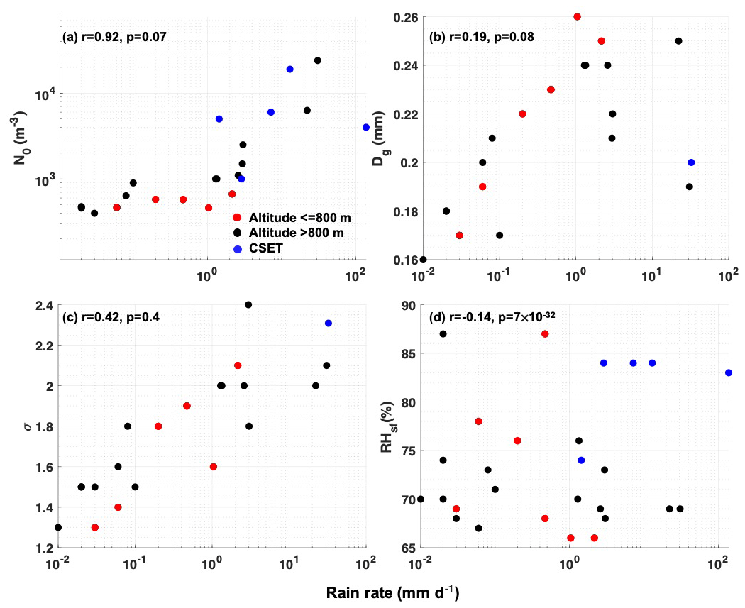
Figure 5 (a) N₀, (b) D_g, (c) σ, and (d) RH_sf are scattered against 10 min leg mean rain rates for 22 cases observed by the P3. Red circles show the cases sampled at 700 ± 100 m altitude, and black circles are cases sampled at altitudes higher than 800 m. Blue circles are for the CSET campaign obtained from Sarkar et al. (2020). Only the average D_g and σ over five CSET cases were available and are shown by single dots in panels (b) and (c). N₀ and RH_sf were available for five cases during CSET and are shown in panels (a) and (d). The correlation coefficients (r) and p value are mentioned in all figures.

3 Results

3.1 Observed rain characteristics

The 10 min (1 Hz) horizontal leg mean rain rates sampled for 20 out of 22 cases on 4, 5, 9, and 10 February (Fig. 3) vary between 0.01 and 3 mm d⁻¹, with a rain frequency between 1 % and 10 %. The other two cases have more intense rain rates of 22 and 31 mm d⁻¹ and rain frequencies of 10 % and 50 %, respectively, as sampled on 9 February at altitudes of 1630 and 2112 m. The leg mean rain rates are calculated using the 1 Hz samples, with rain rates higher than 0.01 mm d⁻¹. The rain frequency is defined as the ratio of the number of raining samples to the total number of raining and non-raining samples within a 10 min horizontal leg. Overall, barring two cases, the rain rates sampled over 20 horizontal legs by the P3 are weak and comparable with rain usually witnessed in stratocumulus clouds.

The highest and lowest rain rates were observed on 9 February (31 mm d⁻¹) and 4 February (0.01 mm d⁻¹), respectively. The low rain rates on 4 February are due to the higher concentration of small raindrop diameters (<200 µm) and almost no raindrops larger than 500 µm when compared to the other days. Similarly, the higher rain rates for the two cases on 9 February are due to the high concentrations of larger drops compared to other cases. In total, 7 out of 22 cases were sampled within ±100 m of cloud base (700 m) while the other cases had sampling altitudes higher than 1.3 km. No rain was detected at any of the 150 m altitude legs (except in one case on 9 February), suggesting that rain either evaporated completely before reaching the surface or was not sampled when it reached the surface.

Vertical and horizontal variability in rain structure is evident in the radar images (Fig. 4), which reveal heterogeneous cloud bases and some heavy precipitation pockets with radar reflectivity higher than +10 dBZ. These heavier precipitating samples partially evaporate before reaching the surface. The more weakly precipitating segments, with smaller radar reflectivities, evaporate completely within the sub-cloud layer. Vertical changes in the rain structure are also evident from in situ observed RSDs measured at different altitudes within the same cloud system. For example, on 9 February, the RSDs shift towards smaller drop sizes as sampling altitudes decrease from 2112 and 1630 to 1500 and 1053 m (Fig. 3c), which could be due to both microphysical and thermodynamic processes in the cloud layer.

3.2 Observed microphysical and thermodynamic variability compared with CSET and RICO

A strong positive correlation is observed between the rain rates and microphysical parameters N₀, D_g, and σ at cloud base (Fig. 5a–c). The higher D_g and σ indicate a higher concentration of larger drops, which account for more liquid water and higher rain rates. While D_g and σ vary modestly (σ by approximately a factor of 2), N₀ varies by several orders of magnitude over 22 P3 cases, with rain rates between 0.01 and 35 mm d⁻¹. The 1 Hz distributions of N₀, D_g, σ, and rain rates are plotted in Fig. 6 to give an overall microphysical statistical characterization for all the P3 cases. The variability in the rain parameters is the lowest on 4 February and highest on 9 February. The P3 cases also show a weak negative correlation between the surface relative humidity (RH_sf) and rain rate (Fig. 5d). This may be due to the downdrafts drying the surface layer and lowering RH_sf. Note that the correlation of RH_sf and the rain rate compared to the microphysical variables is weaker, as indicated by the r values.

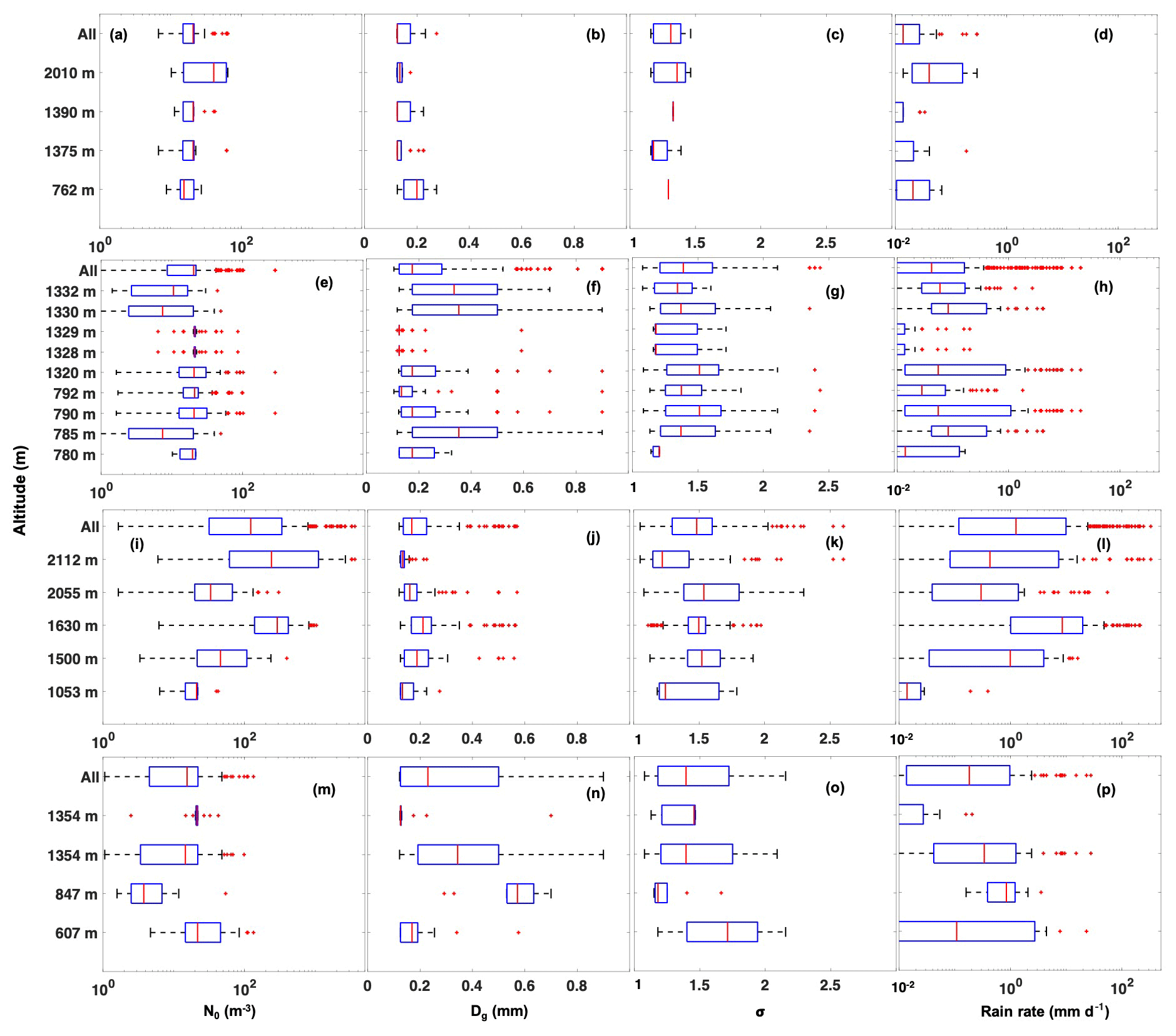
Figure 6 Lognormally fitted 1 Hz rain parameters (a, e, i, m) N₀, (b, f, j, n) D_g, and (c, g, k, o) σ and (d, h, l, p) rain rates are depicted as box plots for all 22 cases on (a–d) 4 February, (e–h) 5 February, (i–l) 9 February, and (m–p) 10 February. The box plots denote the 25th, 50th, and 75th percentiles. The minimum and maximum extents of the whiskers denote the minimum and maximum data points that are not outliers. Outliers are shown with red plus signs (+). Outliers are considered data points outside the $\pm \mathrm{2.7}\times$ standard deviation and 99.3 % coverage.

3.2.1 CSET comparison

Compared to the average P3 cases, the cumulus rain events sampled over five cases during the CSET campaign in the northeastern Pacific Ocean have higher rain rates (1–100 mm d⁻¹), along with higher N₀ (10³–2 ×10⁴ m⁻³) and σ (2.3; Fig. 5a). However, the average D_g for the CSET cases lies within the P3 ranges (Fig. 5b, c). Since D_g and σ did not vary significantly across the five CSET cases, the higher rain rates during CSET could be due mainly to their larger N₀.

A total of four out of five cases during CSET have RH_sf of 84 %, which is higher than for most of the P3 cases. The correlation between the RH_sf and rain rate during CSET is much weaker compared to the P3 cases (Fig. 5d). RH_sf for CSET remains constant at 84 % for rain rates from 1 to 100 mm d⁻¹. That said, it is worth noting that RH_sf measurements during CSET were collected using aircraft observations at 150 m altitude and therefore might differ slightly from the actual surface relative humidity.

The F_eT values during CSET within some heavily precipitating cumulus transects are between 10 and 200 Wm⁻², which is comparable to the P3 F_eT range of 1–350 Wm⁻². The high variability in F_eT for both the P3 and CSET events suggests that the heterogeneity of the cumulus rain processes is a common feature across different ocean basins.

3.2.2 RICO comparison

During the RICO campaign, which was based in the Caribbean like the ATOMIC and EUREC4A field campaigns, the rain rates sampled were stronger than the P3 cases, as in CSET. The cloud base rain rate is 5 mm h⁻¹ during RICO (Fig. 2; Geoffroy et al., 2014). Comparing Fig. 6 with Fig. 2 in Geoffroy et al. (2014), the median rain rates, N₀, and raindrop diameters during RICO at cloud base were much higher than the P3 cases sampled during ATOMIC. Geoffroy et al. (2014) have used a mean volume diameter D_v to describe the variability in their raindrop sizes, which is mathematically different but still comparable to the D_g values that we have used in this study. D_v at 500 m during RICO is 750 µm, which is much higher than D_g values of 200 µm during the P3 cases. Similarly, the median N₀ and rain rates during RICO are 6×10⁴ m⁻³ and 12 mm h⁻¹ at 500 m altitude, compared to the 2×10³ m⁻³ and 3 mm d⁻¹, respectively, averages over all 22 P3 cases. This suggests that the higher rain rates sampled by RICO could have been due to the high N₀ and D_v values when compared to that sampled by the P3.

All flights during RICO were designed to randomly sample clouds above the cloud base (except one on 19 January), and as a result, most flights did not sample any precipitation. But the precipitation samples on 19 January suggest a 6 % reduction in the cloud base rain rate (3 mm h⁻¹) due to rain evaporation (Snodgrass et al., 2009). This roughly translates to 130 Wm⁻² of rain evaporation flux (based on Fig. 10 in Snodgrass et al., 2009) and is comparable to the CSET and the P3 values.

3.3 Modeled rain evaporation in the sub-cloud layer

3.3.1 Vertical distributions of RWC and F_e

The sub-cloud variability in the rain evaporation over 22 cases from ATOMIC and EUREC⁴A is reflected in the vertical profiles of the modeled RWC, rain rate, and F_e in Fig. 7d–f. Cases on 9 February, with their highest rain rates and RWC at the cloud base also have the highest RWC reaching the surface (>0.02 g m⁻³; see Fig. 7d and e). In all, 10 out of 22 cases have RWC higher than 10⁻³ g m⁻³ at the surface, 4 of which are on 9 February.

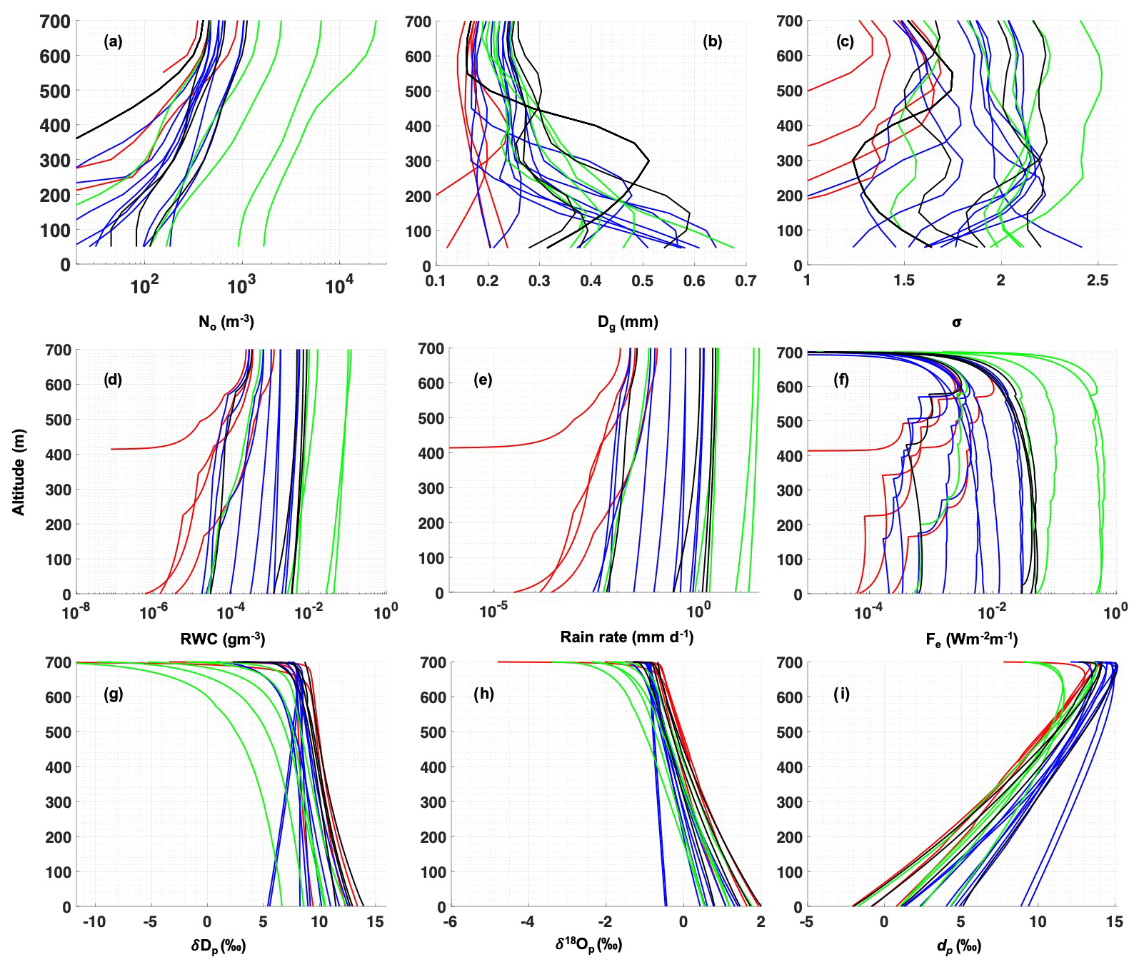
Figure 7 Modeled (a) N₀, (b) D_g, (c) σ, (d) RWC, (e) rain rate, (f) F_e, (g) ${{\mathit{\delta }}^{\mathrm{18}}\mathrm{O}}_{\mathrm{p}}$, (h) δD_p, and (i) d_p vs. height for all 22 P3 cases. The cases on 4, 5, 9, and 10 February are shown with red, blue, green, and black lines, respectively. The modeled RSD is averaged over every 50 m vertical length and then fitted using a lognormal distribution to obtain smooth N₀, D_g, and σ vertical profiles.

In contrast, one case on 4 February evaporates completely within 400 m from the cloud base, with no rain reaching the surface. This is because all drops in the RSD for this case are smaller than 300 µm (Fig. 3a), and smaller drops are more susceptible to evaporation. The cases on 5 and 10 February have RWCs ranging between those on 4 and 9 February, with rain intense enough to reach the surface after partial evaporation.

RWC decreases at a faster rate for cases with smaller RWC at the cloud base, like on 4 February. This leads to an increase in F_e near the cloud base compared to near the surface (Fig. 7f). Conversely, cases with higher RWC at the cloud base, like on 9 February, have a slower rate of decrease in RWC near the cloud base. This is primarily due to the higher concentration of larger drops in these cases that evaporate the most as they reach closer to the surface.

3.3.2 Vertical distributions of N₀, D_g, and σ

The modeled microphysical parameters N₀, D_g, and σ are shown in Fig. 7a–c, where 9 February cases have the highest cloud base N₀ (>1000 m⁻³). The decrease in N₀ with decreasing altitude corresponds well with that in the RWC, as seen earlier.

The net modeled D_g increases and σ decreases from the cloud base to the surface across all 22 P3 cases. Changes in D_g and σ are much smaller than in N₀. In general, D_g increases and σ decreases whenever smaller drops in the RSD evaporate completely. In this way, the complete evaporation of smaller drops makes the RSD narrower and centered over larger D_g. In contrast, if the RSD only has larger drops that only partially evaporate, then the D_g decreases and σ increases, making the RSD wider and centered over smaller D_g.

The higher terminal velocity for bigger drops helps them reach the surface faster, while the longer residence time of slower-falling smaller drops in the sub-cloud layer leads to more complete evaporation of those drops. Thus the lower terminal velocity aids in the overall shift in the RSD towards larger D_g, narrower σ, and lower N₀ from the cloud base to the surface.

3.3.3 Sub-cloud stability due to the vertical distribution of F_e

How bottom heavy or top heavy a profile of F_e is may have an effect on the boundary layer stability. For example, if most moisture from rain evaporation is closer to the cloud base than to the surface (top-heavy profile), then the evaporation-cooled air near the cloud base could mix with the surface-based relatively warmer air more readily. This could potentially help with circulating the surface moisture to the cloud base and help the cloud stay intact.

In contrast, a bottom-heavy rain evaporation profile, where the maximum evaporation-produced moisture is concentrated close to the surface, could lead to a stable configuration. This is because the cooler air close to the surface is not invigorated to mix with the relatively warmer air close to the cloud base. This could inhibit any mixing or vertical transport of moisture from the surface to the cloud base. Such profiles should be more susceptible to cloud dissipation and boundary layer decoupling and may promote the formation of cold pools. Examples of such top- and bottom- heavy profiles, with their relation to boundary layer stability are discussed in Paluch and Lenschow (1991). In this study, we have used the modeled F_e profiles to differentiate between top- and bottom-heavy profiles.

To assess which of the 22 P3 cases is top heavy or bottom heavy, we have summed up F_e values over the bottom 350 m (surface to 350 m altitude) and the top 350 m (350–700 m altitude) to obtain F_top and F_bottom, respectively. The ratio of $F_{\mathrm{bottom}}/F_{\mathrm{top}}$ for all the cases is calculated (Fig. 9). $F_{\mathrm{bottom}}/F_{\mathrm{top}}>\mathrm{1}$ denotes bottom-heavy profiles and $F_{\mathrm{bottom}}/F_{\mathrm{top}}<\mathrm{1}$ top-heavy profiles. All of the cases on 4 February and one on 5 February, where most of the rain evaporated within 100 m from the cloud base, have $F_{\mathrm{bottom}}/F_{\mathrm{top}}$ of 0–0.2 and are therefore top heavy. In total, 11 out of 22 cases have a top-heavy profile, making it more likely for these cloud layers to remain connected with the surface layer.

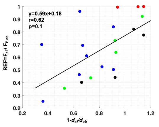
Figure 8 Modeled REF ($=F_{\mathrm{eT}}/F_{\mathrm{p},\mathrm{cb}}$) scattered along the fraction of change in d_p between the cloud base and surface ($\mathrm{1}-d_{\mathrm{sf}}/d_{\mathrm{cb}}$) for 21 out of 22 P3 cases, where the rain reaches the surface after partial evaporation. Circle color codes are red, blue, green, and black for 4, 5, 9, and 10 February, respectively. The black line represents a linear fit of $y=\mathrm{0.59}x+\mathrm{0.18}$, with a correlation coefficient (r) of 0.62 and p value of 0.07. Note that the 4 February cases (red circles) have REF smaller than 1. The x-axis values higher than 1 are for cases where d_cb is positive but d_sf is negative, causing $\mathrm{1}-d_{\mathrm{sf}}/d_{\mathrm{cb}}$ to be higher than 1.

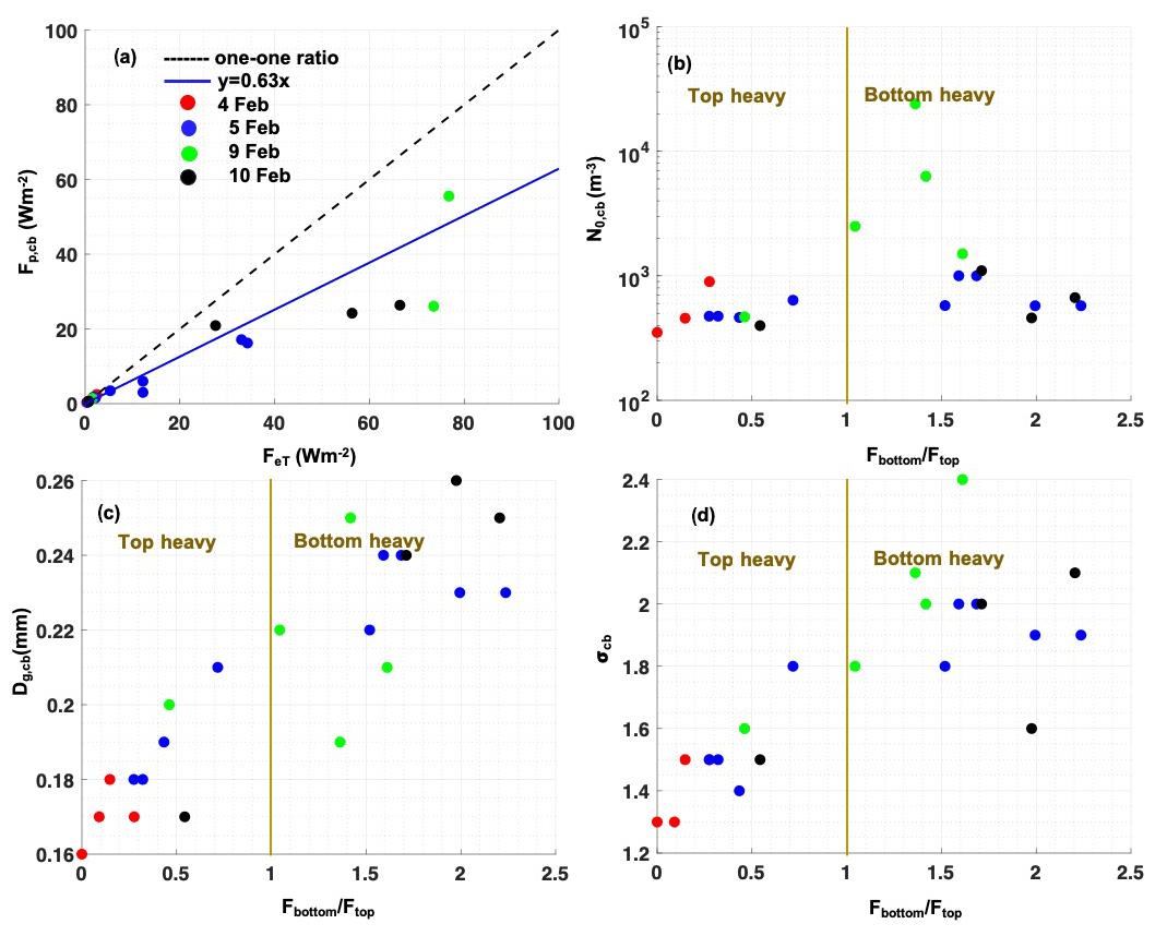
Figure 9 (a) Rain flux at cloud base (F_p,cb) is scattered against the column total sub-cloud rain evaporation flux (F_eT). Only 20 out of 22 cases are shown, excluding the highest two cases on 9 February, with F_eT above 300 Wm⁻². The 4, 5, 9, and 10 February cases are shown in filled red, blue, green, and black circles, respectively. The blue line is the slope through all 22 cases and is 0.63. The dashed black line is the one-to-one ratio line for reference. The $F_{\mathrm{bottom}}/F_{\mathrm{top}}$ ratio is plotted with (b) N_0,cb, (c) D_g,cb, and (d) σ_cb. F_top and F_bottom are the summation of F_e over 350–700 and 0–350 m, respectively. $F_{\mathrm{bottom}}/F_{\mathrm{top}}$ higher than 1 denotes bottom-heavy cases, and $F_{\mathrm{bottom}}/F_{\mathrm{top}}$ less than 1 denotes top-heavy cases, as shown with the gold font.

Next, we evaluate which microphysical conditions are more likely to generate a top- or bottom-heavy F_e profile. Since the F_e structure is dependent on the microphysical state at the cloud base, $F_{\mathrm{bottom}}/F_{\mathrm{top}}$ should also be dependent on the microphysical parameters N₀, D_g, and σ. To demonstrate this here, we have determined the correlation of N₀, D_g, and σ at cloud base with $F_{\mathrm{bottom}}/F_{\mathrm{top}}$ for each case (Fig. 9). A strong correlation is found between $F_{\mathrm{bottom}}/F_{\mathrm{top}}$ and D_g and σ. Comparatively, $F_{\mathrm{bottom}}/F_{\mathrm{top}}$ and N₀ correlate weakly. This might be because the net effect of N₀ is canceled in the numerator and denominator of $F_{\mathrm{bottom}}/F_{\mathrm{top}}$. In all, over the 22 cases, the bottom-heavy sub-cloud profiles, which could be prone to cloud breakup and boundary layer decoupling, have higher values of D_g and σ at the cloud base. Conversely, the top-heavy profiles that could facilitate more intact clouds and higher mixing with the surface layer have smaller D_g and σ values at the cloud base.

A lower RH_sf is also modeled to produce more top-heavy profiles (smaller $F_{\mathrm{bottom}}/F_{\mathrm{top}}$), and vice versa (Fig. 9). This is because the lower the RH_sf, the faster the evaporation rate of drops, leading to the accumulation of moisture and latent flux closer to the cloud base and thus a top-heavy profile.

In summary, high D_g, σ, and RH_sf are all linked to a bottom-heavy energy profile, and vice versa. This shows how the microphysical and thermodynamic parameters of the sub-cloud layer are associated with changing the vertical energy structure and potentially, therefore, affecting the sub-cloud stability.

3.3.4 Microphysical and thermodynamic influence on F_eT and REF

REF in the sub-cloud layer is useful for determining the amount of rain reaching the surface and for formulating the amount of F_eT. F_eT, on the other hand, is an estimate of the column total rain evaporation flux generated in the sub-cloud layer that could indicate the average evaporative cooling rate of the sub-cloud layer. Both REF and F_eT depend on the microphysical and thermodynamic processes in the cloud and sub-cloud layer, as shown by the following model results.

• a.

  Microphysical influence. REF is a strong function of D_g and σ (correlation coefficient $=-\mathrm{0.7}$ and −0.8, respectively). The higher the D_g and σ value at the cloud base, the smaller the REF (Fig. S1f, h). This is because a higher D_g and σ value at the cloud base signifies an RSD with a high proportion of bigger raindrops that are more likely to reach the surface without completely evaporating. Conversely, smaller D_g and σ at the cloud base have higher modeled REF, since smaller drops evaporate more efficiently, thus reducing the overall mass of the rain more. The influence of N₀ on REF is smaller compared to D_g and σ (Fig. S1d). This is because when REF is expanded in terms of N₀, D_g, and σ values, the N₀ appears in the numerator and denominator and almost cancels out.

  F_eT, on the other hand, is strongly impacted by N₀ (and D_g and σ). This is because F_eT is proportional to N₀. In short, while the influence of N₀ is not prominent in REF, its influence dominates F_eT. Most of the P3 cases with higher D_g and σ also have higher N₀. Due to this, lower REF cases are mostly correlated with higher F_eT. But in some cases, like on 9 February, D_g and σ are small but N₀ is large, leading to large REF and large F_eT. Similarly, two cases on 10 February have large D_g and σ values but small N₀, leading to small REF and small F_eT. Overall, the link between REF and F_eT may not be linear due to the underlying microphysical processes. More microphysical observations over shallow rain datasets are required to affirm this connection in a robust way.

• b.

  Thermodynamic influence. The correlation of REF with RH_sf is not as strong as with the microphysical parameters (Fig. S1a, b). But in a sensitivity study, where the microphysical parameters are fixed and RH_sf is varied in 10 % interval jumps, a lower RH_sf is correlated with higher REF (Fig. 10), and vice versa. Accordingly, change in RH_sf is a contributing factor for the changing REF.

  F_eT also increases as RH_sf decreases. As RH_sf decreases and the sub-cloud layer becomes drier, the rate of change in drop size increases ($\frac{\mathrm{d}D}{\mathrm{d}z}$ in Eq. 1). The sensitivity test suggests that for every 10 % increase in RH_sf, F_eT decreases by ≈ 2–6 Wm⁻². For 17 out of 22 cases, RH_sf is between 67 % and 74 %. The remaining five cases are on 5 February and have higher RH_sf values of 76 %–87 %. Holding the microphysical parameters constant, an increase in RH_sf from 67 % to 87 % would decrease the REF and F_eT by 60 % and 53 %, respectively.

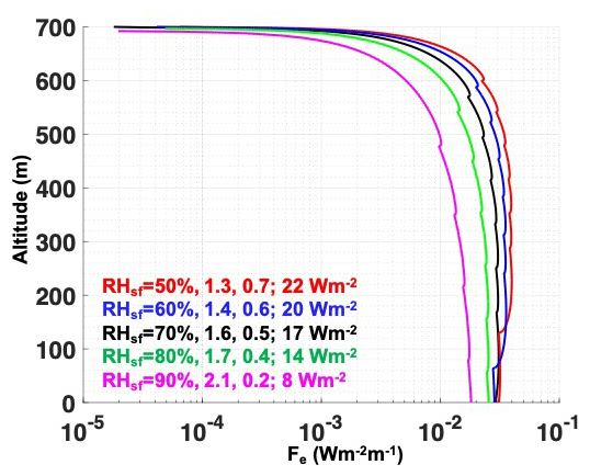
Figure 10 F_e profiles modeled with altitude for RH_sf values of 50 % (red), 60 % (blue), 70 % (black), 80 % (green), and 90 % (magenta), respectively. The RH_sf is followed by the $F_{\mathrm{bottom}}/F_{\mathrm{top}}$, REF, and F_eT values in the legend.

3.3.5 F_eT vs. F_p,cb

A scatterplot between F_p,cb and F_eT is shown for 20 of 22 cases (Fig. 9a). The other two cases are from 9 February, where F_p,cb values are higher than 500 Wm⁻² and are not shown in the figure for clarity. Moreover, 5 out of 22 cases on 4 and 5 February, where rain evaporates completely, have F_eT equal to F_p,cb. Otherwise, as F_p,cb increases, F_eT and hence REF values tend to become smaller.

The slope of F_p,cb versus F_eT shown in Fig. 9a is 0.63, indicating that on average 63 % of the rain mass sampled by the P3 has evaporated in the sub-cloud layer. The magnitude of F_eT is between 15 and 352 Wm⁻² for 9 out of 22 cases. This is analogous to 2–50 K d⁻¹ of net evaporative cooling rate for the sub-cloud layer, which is estimated using $\frac{\mathit{\delta }T}{\mathit{\delta }t}=\frac{\mathrm{1}}{{\mathit{\rho }}_{\mathrm{a}}{c}_{\mathrm{p}}}\frac{F_{\mathrm{eT}}}{H}$, with ρ_a,c_p and H as the density of air, the heat capacity of dry air, and the cloud base height. This is comparable to a typical longwave radiative cooling rate over the marine boundary layer depth of 4–10 K d⁻¹ and should therefore contribute significantly to the boundary layer energy budget in shallow convective environments where rain is present.

3.4 Rain evaporation analysis using rain isotope ratios δD_p and δ¹⁸O_p

3.4.1 Modeled δD_p, δ¹⁸O_p and d_p for the P3 cases

Changes in δD_p, ${{\mathit{\delta }}^{\mathrm{18}}\mathrm{O}}_{\mathrm{p}}$, and d_p are modeled for all 22 P3 cases (Fig. 7g–i). As rain evaporates in the sub-cloud layer, the modeled δD_p and ${{\mathit{\delta }}^{\mathrm{18}}\mathrm{O}}_{\mathrm{p}}$ increase, and d_p decreases towards the surface. The decrease in d_p is caused by the preferential evaporation of D in the water molecule, owing to their lower mass, higher vapor pressure, and larger diffusivity compared to ¹⁸O, leaving the rain less enriched in δD_p compared to ${{\mathit{\delta }}^{\mathrm{18}}\mathrm{O}}_{\mathrm{p}}$.

The P3 cases with the higher modeled surface d_p have either high RH_sf (>75 %), large D_g and σ (compared to average P3 values), or both. The model also shows a positive correlation between the fractional change in d_p from cloud base to the surface ($\mathrm{1}-d_{\mathrm{p},\mathrm{sf}}/d_{\mathrm{p},\mathrm{cb}}$) and REF for 22 P3 cases (Fig. 8). This is logical, since a small REF suggests a smaller fraction of rain mass evaporation, which would correspond to a smaller change in d_p from the cloud base to the surface.

3.4.2 Comparison of model results with surface δD_p, δ¹⁸O_p, and d_p observations

The surface-based observations of δD_p, ${{\mathit{\delta }}^{\mathrm{18}}\mathrm{O}}_{\mathrm{p}}$ (Fig. S3), and d_p (Fig. 11a) from Ron Brown, the BCO, and Meteor range between 0 ‰–20 ‰, − 2.5 ‰–1.2 ‰, and 4 ‰–18 ‰, respectively. δD_p for the BCO is slightly smaller than for Ron Brown and Meteor, and the Meteor d value is slightly smaller compared to the BCO and Ron Brown. Overall, these values correspond well to those across other platforms during the EUREC⁴A and ATOMIC campaign (refer to Bailey et al., 2023). In particular, the rain sampled by Ron Brown shows surface rain rates of 1–5 mm h⁻¹ at an average RH_sf of 85 %. These values are higher compared to the average P3 rain rate and RH_sf.

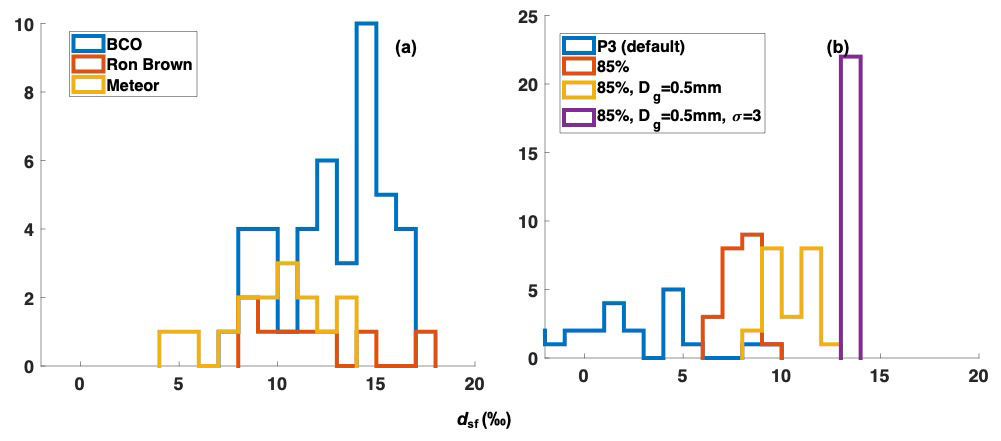
Figure 11 (a) Histograms of surface d_p (d_sf) observed by Ron Brown (red), Meteor (yellow), and BCO (blue). (b) Histograms of modeled surface d_p for all the P3 cases run at observed cloud base D_g (0.16–0.26 mm), σ (1.2–2.4), d_p (7 ‰–15‰), and RH_sf (66 %–87 %; where blue is the default condition). Histograms of the P3 cases run at default D_g, σ, and d_p levels but at RH_sf of 85 % (red). Histograms of the P3 cases run at default σ and d_p levels but at RH_sf and D_g of 85 % and 0.5 mm, respectively (yellow). Histogram of modeled d_sf at cloud base D_g, σ, d_p, and RH_sf of 0.3 mm, 3 ‰, 14 ‰, and 85 %, respectively (purple).

The modeled d_p values at the surface for the P3 cases are between −2 ‰ and 9 ‰ (Fig. 11b; blue line). Of these, the cases with RH_sf values higher than 73 % have the higher d_p between 3 ‰ and 9 ‰. These higher modeled d_p cases overlap with some of the Ron Brown observations of 8 ‰–18 ‰. Moreover, when all P3 cases are run at an increased RH_sf level of 85 % to replicate the Ron Brown thermodynamic conditions, the modeled surface d_p value increases to 6 ‰–10 ‰ (Fig. 11b; red line). This finding is consistent with the idea that we would expect measurable rain with higher d_p to reach the surface when RH_sf is higher.

Similarly, the modeled d_p also shifts closer to the Ron Brown values when the model is run at larger D_g and σ values compared to the P3 ranges. Running the model at D_g to 0.5 mm and RH_sf of 85 %, and keeping σ within the P3 range (1–2.5), the modeled surface d_p increases to 8 ‰–13 ‰ (Fig. 11b; yellow line). Furthermore, increasing σ to 3, along with D_g and RH_sf, also further increases the modeled d_p to 14 ‰ (Fig. 11b; purple line). The choice of increasing σ to 3 is consistent with the upper range of σ during RICO (Fig. 4 in Geoffroy et al., 2014).

A higher D_g and σ at the cloud base lead to a lower fraction of rain mass evaporation or lower REF. A lower REF then leads to less change in d_p between the cloud base and surface and hence larger surface d_p. The evaluation of the model outputs against the station observations also lends credibility to our model. These experiments demonstrate the strong thermodynamic and microphysical influence of the sub-cloud layer on the surface d_p. Equivalently, the reliability of using d_p as a metric for sub-cloud rain evaporation studies is also demonstrated.

Note that both δ_p and d_p values are independent of N₀ and only depend on D_g and σ. This can explain why an “amount effect” (Dansgaard, 1964) is not always present in low-latitude isotopic datasets. The amount effect suggests that for a given rain sample, if the rain rate is high, then δ_p should be low, and vice versa. However, this may not always hold true for all microphysical conditions. If N₀ is large and D_g and σ values are small, then the rain rate could still be high due to its strong sensitivity to N₀. But, due to the small D_g and σ, the δ_p will also be high. Similarly, if N₀ is small and D_g and σ are large, then both the rain rate and δ_p will be low. Consequently, the amount effect may not be appropriate for explaining all rain events, especially when the microphysical variability is pronounced.

3.5 Water vapor isotope ratio variations

Next, we assess whether raindrop evaporation during the P3 cases could cause a detectable isotopic change in the sub-cloud layer water vapor. The maximum simulated F_e, associated with 9 February, was 0.7 Wm⁻² m⁻¹, which corresponds to a moisture flux of $\mathrm{3.1}\times {\mathrm{10}}^{-\mathrm{4}}$ g m⁻³ s⁻¹ ($\frac{F_{\mathrm{e}}}{L}$). Over the course of a 15 min rain shower, and neglecting dilution or advection, this flux would cause a change in absolute humidity of about 0.3 g m⁻³ ($\frac{F_{\mathrm{e}}\times \mathrm{900}\mathrm{s}}{L}$). Since the measured absolute humidity on this day was 15 g m⁻³, these results indicate that rain evaporation may have contributed 2 % to the moisture content of the sub-cloud layer. Given the observed δD_v of −71 ‰ and the simulated δD_e of 5 ‰, we can estimate the isotopic change in the sub-cloud layer water vapor due to raindrop evaporation from Eq. (11), which yields an isotopic change of 1 ‰. Since variations of 1 ‰ δD_v are readily detectable with today's airborne water vapor isotopic analyzers, we surmise that the rain on 9 February should have caused a measurable shift in the water vapor isotope ratios of the sub-cloud layer.

4 Conclusions and discussion

This study evaluates shallow rain evaporation characteristics in the North Atlantic Ocean near Barbados using a one-dimensional sub-cloud rain evaporation model initialized by observations from the EUREC⁴A and ATOMIC campaign. The focus is on 22 raining cases sampled by the P3, where the cloud base leg mean rain rates and RWC are between 0.01–31 mm d⁻¹ and 0.0001–0.1 g m⁻³, respectively. These cases show interesting variability in their sub-cloud rain evaporation characteristics and their dependence on the microphysical and thermodynamic state of the boundary layer.

The total rain evaporation flux (F_eT) over 22 P3 cases is modeled to be 15–352 Wm⁻², which is close to the 3 d mean 100 Wm⁻² latent heat flux at 200 m altitude that was measured remotely from aboard R/V Maria S. Merian, another EUREC⁴A research vessel that sampled to the south of the P3 study region (Stevens et al., 2021). The F_eT for the P3 cases are also comparable with estimates from ASTEX (42 Wm⁻²), RICO (130 Wm⁻²), and CSET (10–200 Wm⁻²). These differences and the variability, especially between the P3 cases and during RICO and CSET, are a result of differences in their RH_sf, D_g, σ, and N₀ values in the sub-cloud layer.

F_eT of 15–352 Wm⁻² over a 700 m deep sub-cloud layer is equivalent to 2–50 K d⁻¹ of evaporative cooling. This is comparable to the typical stratocumulus cloud-top radiative longwave cooling (4–10 K d⁻¹) and with the rain evaporation cooling rate at cloud base in the marine sub-cloud stratocumulus deck of 2–20 K d⁻¹ (shown in Wood, 2005). This shows that shallow rain evaporation can contribute significantly to the local energy budget and sub-cloud cooling rates.

Depending on the vertical distribution and magnitudes of F_e, the sub-cloud layer could be energetically top or bottom heavy and potentially influence the boundary layer stability through downdrafts or decoupling. In total, 11 out of 22 cases have most of their rain evaporated closer to the surface. This bottom-heavy configuration should inhibit mixing with the warmer air near the cloud base and therefore should aid the boundary layer in decoupling faster. This could also facilitate cold-pool formation.

In contrast, the other 11 cases that are top heavy accumulate moisture near the cloud base and are more prone to mixing with warmer air below. This could lead to a mixed boundary layer in which clouds could remain intact for longer. A follow-up modeling study is needed to confirm these processes and to see the degree to which the boundary layer stability depends on the representation of rain evaporation within the model.

A top-heavy F_e profile is linked with lower D_g and σ at the cloud base. This makes physical sense, since a lower D_g and σ at the cloud base would mean that the raindrops are small and the RSD is narrow enough for the drops to evaporate closer to the cloud base. Conversely, a bottom-heavy F_e profile is linked with higher D_g and σ values due to the higher concentration of larger drops that reach the surface without evaporating completely. This emphasizes the influence of microphysical characteristics of rain at cloud base on the sub-cloud vertical F_e profile.

Additionally, given the constant microphysical parameters at the cloud base, a top-heavy F_e profile is also linked with lower RH_sf values. This is because lower RH_sf increases the rate of rain evaporation, especially for smaller drops, facilitating more accumulation of moisture close to the cloud base. In contrast, higher RH_sf favors bottom-heavy F_e profiles. This depicts the influence of thermodynamic conditions, in addition to microphysical conditions, in modulating the vertical rain evaporation flux distribution.

The model also shows that, on average, 63 % of the rain mass evaporated in the sub-cloud layer for 22 P3 cases. Most of these cases with higher REF are associated with smaller D_g, σ, and RH_sf values, and vice versa. However, the effect of RH_sf on REF is lower compared to D_g and σ.

Moreover, if N₀, D_g, and σ values are all large, then F_eT tends to be large and REF small, as seen for most of the 22 P3 cases. However, there are cases when D_g and σ are large but N₀ is small. This leads to small F_eT and small REF. A few cases also have small D_g and σ but large N₀ values, resulting in fairly large F_eT and large REF. Effectively, therefore, the fraction of rain evaporated (or REF) and the amount of rain evaporated (or F_eT), are more intrinsically dependent on the RSD microphysical parameters rather than on the bulk RWC itself.

In terms of the rain isotopic composition, our results show that sub-cloud conditions with higher RH_sf, higher D_g, and σ values are prone to higher surface d_p. This is because a higher RH_sf and higher cloud base D_g and σ lead to less evaporation of raindrops and low REF and, thereby, smaller changes in d_p between the cloud base and the surface. In general, the REF varies linearly with the fractional change in d_p between the cloud base and the surface (or $\mathrm{1}-d_{\mathrm{p},\mathrm{sf}}/d_{\mathrm{p},\mathrm{cb}}$). Isotope differences in the rain between the cloud base and the surface thus provide an independent measure of REF.

The model results also suggest why the amount effect or a negative correlation between rain rate and δ_p is not always found in low latitudes. It is a result of the underlying microphysics of the RSD. If the high rain rate is due to large D_g and σ values, then the δ_p should be low due to the small REF. In contrast, if the rain rate is high because of high N₀ and small D_g and σ values, then δ_p should be high due to high REF. This is especially relevant for shallow rain regimes where microphysics play a significant role in determining rain characteristics.

In general, our isotope-initialized microphysics-resolved model performs reliably well in characterizing the sub-cloud rain evaporation in the shallow rain regime sampled during the ATOMIC and EUREC⁴A campaign. This model also only requires in situ microphysical and rain isotope observations and is independent of any remotely sensed rain observations. However, a comparison between rain evaporation evaluated from remote-sensing platforms (e.g., millimeter wavelength radars) and our in-situ-based model could be useful for suitable error analysis.

The results from the model emphasize the role of microphysical and thermodynamic processes in accurately simulating sub-cloud rain evaporation. The variability in the modeled rain evaporation fluxes across 22 P3 cases also highlights the need for more samples in similar shallow cloud regimes for a more robust statistical interpretation that could be used to evaluate general circulation model (GCM) parameterizations. The model also provides an opportunity to extend the rain evaporation study from other field campaigns conducted over different ocean basins and different seasons, which is crucial for a wider understanding of sub-cloud rain processes.