the Creative Commons Attribution 4.0 License.
the Creative Commons Attribution 4.0 License.
 | 24 Jan 2023
Monitoring sudden stratospheric warmings under climate change since 1980 based on reanalysis data verified by radio occultation
Ying Li
Gottfried Kirchengast
Marc Schwaerz
Yunbin Yuan
We developed a new approach to monitor sudden stratospheric warming (SSW) events under climate change since 1980 based on reanalysis data verified by radio occultation data. We constructed gridded daily mean temperature anomalies from the input fields at different vertical resolutions (basic-case full resolution, cross-check with reanalysis at 10 stratospheric standard pressure levels or 10 and 50 hPa levels only) and employed the concept of threshold exceedance areas (TEAs), the geographic areas wherein the anomalies exceed predefined thresholds (such as 30 K), to monitor the phenomena. We derived main-phase TEAs, representing combined middle- and lower-stratospheric warming, to monitor SSWs on a daily basis. Based on the main-phase TEAs, three key metrics, including main-phase duration, area, and strength, are estimated and used for the detection and classification of SSW events. An SSW is defined to be detected if the main-phase warming lasts at least 6 d. According to the strength, SSW events are classified into minor, major, and extreme. An informative 42 winters' SSW climatology (1980–2021) was developed, including the three key metrics as well as onset date, maximum-warming-anomaly location, and other valuable SSW characterization information. The results and validation against previous studies underpin that the new method is robust for SSW detection and monitoring and that it can be applied to any quality-assured reanalysis, observational and model temperature data that cover the polar region and winter timeframes of interest, either using high-vertical-resolution input data (preferable basic case), coarser standard-pressure-levels resolution, or (at least) 10 and 50 hPa pressure level data. Within the 42 winters, 43 SSW events were detected for the basic case, yielding a frequency of about 1 event per year. In the 1990s, where recent studies showed gaps, we detected several events. Over 95 % of event onset dates occurred in deep winter (December–January–February timeframe, about 50 % in January), and more than three-quarters have their onset location over northern Eurasia and the adjacent polar ocean. Regarding long-term change, we found a statistically significant increase in the duration of SSW main-phase warmings of about 5(±2) d over the climate change period from the 1980s to the 2010s, raising the average duration by nearly 50 % from about 10 d to 15 d and inducing an SSW strength increase of about 40(±25) million km2 days from about 100 to 140 million km2 days. The results are robust (consistent within uncertainties) across the use of different input data resolutions. They can hence be used as a reference for further climate-change-related studies and as a valuable basis for studying SSW impacts and links to other weather and climate phenomena, such as changes in polar-vortex dynamics and in mid-latitude extreme weather.
- Article
(16063 KB) - Full-text XML
- BibTeX
- EndNote


Sudden stratospheric warming (SSW) describes an atmospheric-variability phenomenon at a daily-to-monthly scale where temperature in the middle stratosphere (about 30 km or 10 hPa) increases rapidly (>30 to 40 K) within a couple of days in sub-polar and polar regions (McInturff, 1978; Butler et al., 2015; Baldwin et al., 2020). In extreme cases, SSW temperature anomalies can reach more than 70 K relative to the long-term mean. During a strong event, the westerly zonal-mean zonal winds of the polar vortex can reverse, and the three-dimensional polar vortex can undergo a displacement or split (Charlton and Polvani, 2007; Hu et al., 2015; Butler and Gerber, 2018). SSWs are generally understood to be caused by tropospheric planetary waves, which penetrate into the stratosphere and then influence the stratospheric polar vortex (McInturff, 1978; Thompson et al., 2002; Labizke and Kunze, 2009). Solar radiation is also believed to be one of the causes of stratospheric warming (McInturff, 1978; Garfinkel et al., 2015). SSWs usually occur in the polar regions of the Northern Hemisphere (beyond 60∘ N), while they rarely occur in the southern polar region due to less tropospheric-planetary-wave activity (Van Loon et al., 1973). We therefore focus on SSWs of the Northern Hemisphere in this SSW-ensemble-based analysis over multiple decades since 1980.
SSWs are an important indicator of polar-winter variability. They strongly interact with the troposphere (Hitchcock and Simpson, 2014; Lehtonen and Karpechko, 2016), mesosphere (Vignon and Mitchell, 2015; Singh and Pallamraju, 2015), and the upper atmosphere and ionosphere (Jonah et al., 2014; Kakoti et al., 2020) through atmospheric circulations and thermodynamics that mediate stratosphere–mesosphere–thermosphere couplings. The warming in the middle stratosphere will, on the one hand, propagate downwards to lower altitude levels and cause longer-lasting warming in the lower stratosphere (Hitchcock and Simpson, 2014). Some extreme events have impacts into the deep troposphere and cause a large area of blocking high pressure and subsequently cause cold weather in the regions of northern Europe, eastern Asia, and northern America (Cattiaux et al;., 2010; Yu et al., 2015; Tyrlis et al., 2019; Hall et al., 2021). Some SSW events also cause the cooling of the mesosphere and elevated stratopause (Holt et al., 2013; Vignon and Mitchell, 2015; Singh and Pallamraju, 2015). In the ionosphere, the distribution of election density is found to be changed as a response to SSW (Nayak and Yigit, 2019; Kakoti et al., 2020). Due to atmospheric meridional circulation, the tropical stratosphere is found to cool at the same time as there is polar stratospheric warming (Yoshida and Yamazaki, 2011; Dhaka et al., 2015). Regarding atmospheric composition and chemistry, such as the distribution of ozone, water vapor, and energetic particle precipitation, these are found to be changed as well (Kuttippurath and Nikulin, 2012; Ayarzagüena et al., 2013; Holt et al., 2013).
Given this variety of strong interactions of SSWs, it is important to accurately observe, detect, and monitor such events, including their possible transient changes under climate change. Accurate SSW observations require high-quality data to be sufficiently dense in the polar stratosphere. However, observations in these regions are notoriously sparse. Early studies used radiosonde or rocketsonde to observe SSWs. However, both datasets are generally land limited and cannot provide high-vertical-resolution and high-quality data throughout the lower, middle, and upper stratosphere. With the advent of the satellite era in the 1970s, it is possible to put instruments, such as microwave limb sounders, infrared spectrometers, and radiometers, on satellites in order to observe the atmosphere globally (e.g., Hitchcock and Shepherd, 2013; Noguchi et al., 2020). However, satellite passive-sounding data come in the form of radiances, which only allow coarse vertical resolutions, limiting the accurate conversion to altitude-resolved temperature or wind profiles, which are key variables for reliable SSW monitoring.
With the advances of atmospheric data assimilation systems, reanalysis data have become quite a reliable data source for long-term atmospheric analyses due to the advantages of their regular sampling in space and time and their capability to provide reasonably reliable data up to the stratopause (e.g., Charlton and Polvani, 2007; Yoshida and Yamazaki, 2011; Butler et al., 2017; Butler and Gerber, 2018; Hersbach et al., 2020). However, reanalysis data may have some inhomogeneities and irregularities in the long term due to episodic observation system updates and adding in a diversity of new streams of observation datasets over multi-decadal time ranges; they are not a direct, long-term, consistent observation of the atmosphere. It is hence important to verify results based on reanalysis data by complementary use of observational data records with better long-term stability.
In addition to the sparsity of robust observation techniques, SSWs also have no community-agreed standard definition for reliable detection and monitoring. Butler et al. (2015) provided a detailed overview on the history of various SSW definitions and calculated SSW frequency to cross-evaluate nine different definitions based on reanalysis data. Their results suggest that frequencies obtained using different definitions vary a lot, from about 0.4 to 0.9 events per year, and the onset (or maximum-anomaly) dates of major SSWs for each definition may differ substantially as well. Reasons for these discrepancies are mainly related to method design. Each definition has its own unique characteristics. For example, definitions based on wind reversal may focus more on polar vortices, and definitions based on stratosphere–troposphere impacts may focus more on the impacts of SSW on the troposphere. Definitions based on one latitude or region are more sensitive to such variations than definitions based on larger domains (Butler et al., 2015). Also, the details of implementation in selecting detection variables, latitude, altitude, thresholds, and background climatology information can make the results different. These discrepancies in SSW definitions make consistent statistical assessments of SSWs more difficult. Furthermore, at the side of atmospheric physics and dynamics, the analysis of other weather and climate phenomena that relate to SSWs is more limited in scope if accurate SSW diagnostics and monitoring cannot be given.
To help mitigate these current limitations, we propose and apply a new method to monitor SSW events over the 1980 to 2021 Northern Hemisphere winter half years using Global Navigation Satellite System (GNSS) radio occultation (RO) data (Angerer et al., 2017) and ECMWF reanalysis fifth-generation (ERA5) data (Hersbach et al., 2020), developing a 42-year SSW event climatology and evaluating SSW event characteristics.
GNSS RO is an atmospheric remote-sensing technique that provides vertical atmospheric profiles, such as of temperature, density, and pressure (Kursinski et al., 1997; Kirchengast, 2004). RO data have distinctive advantages of high vertical resolution, high accuracy, long-term consistency, and global coverage (Anthes, 2011; Steiner et al., 2011). The vertical resolution of RO in the stratosphere is about 1 km, which is very high compared with other global observation techniques. Validation results against radiosondes and verification with (re)analysis data (that generally assimilate RO data) suggest that the data are of small discrepancy (<2 K) in the upper troposphere and lower stratosphere (Scherllin-Pirscher et al., 2011a, b; Ladstädter et al., 2015; Steiner et al., 2020a, b). RO data from different satellites can be combined without inter-calibration, which make them very suitable for climate-related studies (Foelsche et al., 2011; Angerer et al., 2017; Steiner et al., 2020a). Finally, since a multi-RO satellite observation record started in 2006 (Angerer et al., 2017), the geographic data coverage is sufficiently dense for monitoring and analyzing regional-scale phenomena such as SSWs from that time onwards.
Complementary to reanalysis datasets, which also offer dense coverage, RO reprocessing datasets hence feature accurate and long-term, stable observational records of climate benchmark quality (Steiner et al., 2020a), allowing for stable conditions for SSW monitoring over decades. Therefore, given the complementarity of these single-source, long-term, consistent benchmark observations to reanalyses (Bosilovich et al., 2013; Parker, 2016; Simmons et al., 2020; Hersbach et al., 2020), RO data are ideal for SSW studies.
An initial use of RO data for SSW study was by Klingler (2014), who was the first to use the data to examine the temperature changes during the 2009 SSW event. A couple of studies have also used RO data to analyze their impacts on gravity wave activity, the ionosphere, and also the tropical atmosphere (Yue et al., 2010; Lin et al., 2012; Dhaka et al., 2015). However, use for longer-term SSW detection and monitoring is a next step to be made. We have carried out an initial study (Li et al., 2021), where we used RO data and ERA5 data to develop a new threshold-exceedance-area-based approach to monitor and characterize the strong and well-known 2009 SSW event. We revealed, in principle, high potential for the new method to be used for detection and monitoring of SSWs over multi-decadal timeframes as well.
In this study, building upon the initial Li et al. (2021) work, we apply the approach over 14 winters of RO data (2007 to 2020) and 42 winters (1980 to 2021) of ERA5 data, using the former reprocessing record to cross-verify the latter reanalysis dataset for the purpose. We derive robust SSW characterization metrics and a new definition based on temperature field data, and we apply the new method for SSW detection, classification, and monitoring and to explore long-term changes in their characteristics under the recent climate change.
The paper is structured as follows. Section 2 briefly assesses current SSW detection methods and definitions and then summarizes the features of our new method. Section 3 introduces the data and methodology of our method, and Sect. 4 presents and discusses the results. Finally, conclusions are given in Sect. 5.
2.1 Current definitions
A sudden stratospheric warming (SSW) was first observed by Richard Scherhag using radiosonde measurements in Berlin, Germany, in January–February 1952 (Scherhag, 1952), when he found an abrupt temperature increase in the stratosphere. After about a decade, the World Meteorological Organization (WMO) Commission for Atmospheric Sciences (CAS) developed an international SSW monitoring program called STRATALERT based on available radiosonde and rocketsonde observations (WMO/IQSY, 1964). The WMO CAS suggested that an SSW warning be provided when a sudden and unusual increase in temperature at 30 km or above is detected.
With time ongoing and after more events were observed, it was well recognized that many SSWs occurred along with wind reversals and/or polar-vortex displacement or splits (Johnson et al., 1969; Charlton and Polvani, 2007). Since the 1970s, many studies combined temperature increases and wind reversals to detect SSWs, though detailed implementation and thresholds used are different (e.g., Schoeberl, 1978; Labitzke, 1981). An often-used definition at this stage was suggested by McInturff (1978). He defined that an SSW event occurred if temperature increased by more than 25 K, and the event was defined as a major one if a stronger temperature increase was jointly observed with a wind reversal.
Since wind reversal is one of the most important features of SSWs, many studies suggest using wind reversal for detecting major SSW events (e.g., Charlton and Polvani, 2007; Hu et al., 2015; Butler et al., 2015, 2017; Butler and Gerber, 2018). One of the most-often-used definitions is the one from Charlton and Polvani (2007) (denoted as CP07 hereafter): a major SSW occurs when the zonal-mean zonal winds at 60∘ N at the 10 hPa level become easterly during wintertime. Wind reversal is a simple and robust definition and is useful in studying many influences triggered by SSW. In addition to wind reversal definitions, there are also studies that used vortex moment, which is another important characteristic of the warmings, to detect SSW events (Seviour et al., 2013; Mitchell et al., 2013). Furthermore, polar-cap or zonal-mean stratospheric geopotential height anomalies at 10 hPa were used to detect SSW events (Baldwin and Thompson, 2009; Gerber et al., 2010).
Butler et al. (2015) tested the sensitivity of SSW detection results to nine definitions and found that SSW frequencies obtained under these different definitions varied from 0.35 to 0.91 events per year and that the onset dates also varied substantially. There are several reasons for these discrepancies. First of all, while SSWs usually occur along with wind reversal or polar-vortex change, this is not always the case. Several studies detected significant stratospheric warming but did not simultaneously detect wind reversals at the commonly used 60 or 65∘ N latitude. For example, Mitchell et al. (2013), who used vortex geometry for diagnosing SSW, found half of their events to be inconsistent with those obtained by CP07. Therefore, definitions based on different parameters can make detection results different. Secondly, single-latitude and/or single-altitude definitions, such as for wind reversal, may miss some important SSWs that occurred primarily in other latitude–altitude domains (e.g., Manney et al., 2015; Singh and Pallamraju, 2015). Thirdly, definitions can be sensitive to background climatology and specific thresholds used, especially if based on broad polar-cap-mean anomalies. Finally, current definitions either use zonal-mean or polar-cap-mean results, which do not enable dynamical 3D tracking of such events, and therefore can only provide information of onset date. However, the dynamic location and strength information is rather important for studies on SSWs' interactions with other phenomena, both regarding causes and impacts. Furthermore, SSW is also not a one-level phenomenon; its occurrence and impacts are related to almost the whole stratosphere.
In view of the studies we surveyed and from our own initial study (Li et al., 2021), we suggest that a new SSW monitoring method should build upon the temperature field that directly expresses the sudden stratospheric warming for quantifying this anomalous thermal behavior as the primary SSW fingerprint. It should robustly detect and characterize SSW events, from minor to extreme ones, as a whole phenomenon without being unduly sensitive to details. The method should also be readily applicable to both observational and model data (as long as they are sampled sufficiently densely, preferably grid based) and should not need adjustment to any specific suitable dataset (e.g., a particular reanalysis, atmospheric forecast, climate model simulation, or observational data record). Finally, upon detection, the SSW monitoring metrics should be informative regarding the duration, strength, and dynamic location of each SSW in order to facilitate long-term change monitoring and effective use in cause-and-impact studies. Implementing these suggestions, we propose our new method and definitions in Sect. 2.2.
2.2 New method and its features
SSWs, as reflected by their name, were originally determined by their strong and rapid temperature increase. Therefore, in the method proposed here, we use temperature as the key variable for the diagnostics. Compared to wind- and polar-vortex-based definitions, temperature is a more accessible parameter that can be obtained from various observations. In addition, temperature is a well-related parameter when analyzing SSW relations to other phenomena in the troposphere, as well as in the mesosphere, thermosphere, and ionosphere. Many studies chose to use temperature solely or combined it with wind field changes in studying the impacts of SSWs (e.g., Zhou et al., 2002; Siskind et al., 2010; Manney et al., 2015; Jonah et al., 2014; Kakoti et al., 2020; Singh and Pallamraju, 2015; Vignon and Mitchell, 2015). Also, further thermodynamic variables, particularly air density and pressure, are often readily available for auxiliary co-information (Li et al., 2021).
Based on temperature changes, we designed the method to be fairly insensitive to temperature field details. Firstly, we use robust stratospheric temperature anomaly profiles or pressure level data at any data location (such as a grid point) as the basis for expressing the local warming, using an anomaly technique that has been proven to be useful and robust in diagnosing many other climate and atmospheric change phenomena, such as those related to tropical cyclones (Biondi et al., 2015), atmospheric blocking (Brunner et al., 2016), or thermal imprints of wildfires (Stocker et al., 2021). As described in detail by Li et al. (2021) and as summarized in Sect. 3 below, we then calculate vertical mean anomalies in selected stratospheric layers or at selected levels and categorize them into large-scale grid cells covering the polar region, based on which we compute, on a daily basis throughout wintertime, temperature threshold exceedance areas and related metrics, which serve as the basis for SSW detection and monitoring.
In establishing SSW climatologies (i.e., cataloguing SSW events over a multi-decadal period), previous studies generally only provide information about onset dates and vortex splits or displacement. In the climatology we build based on the new method, we can provide SSW event onset date (of maximum middle-stratosphere warming), duration, exceedance area, and strength, as well as complementary day-by-day dynamic tracking of the center location, associated maximum warming, and areal extent of the exceedance area. Furthermore, most previously published climatologies do not yet reach beyond 2013 and miss some events over the 1990s decade, while we provide a climatology continuously extending from 1980 to 2021 and hence filling these gaps.
Compared to our initial method introduction and its careful evaluation in Li et al. (2021), which was based on the strong 2009 SSW event only, we focused on and refined the diagnostics for the metrics so that they now fully deploy for multi-decadal detection, classification, and monitoring. The details on data and methodology are described next in Sect. 3.
3.1 RO data
Since 2001, a continuous record of RO data is provided by GNSS RO missions, including the Challenging Mini-satellite Payload mission (CHAMP; Wickert et al., 2001), followed by the Gravity Recovery and Climate Experiment (GRACE, Wickert et al., 2005), and the Constellation Observing System for Meteorology, Ionosphere, and Climate (COSMIC; Schreiner et al., 2007), the European Meteorological Operational satellites (MetOp; Luntama et al., 2008), the Chinese FengYun-3C operational satellite (Sun et al., 2018), and others. Since the launch of COSMIC, which was a constellation of six satellites, around mid-2006, there has been sufficient coverage with RO event observations for regional-scale studies such as those on SSWs. Therefore, in this study, we use the RO data record from the wintertime of 2006–2007 onwards.
We use the atmospheric profiles from the Wegener Center for Climate and Global Change (WEGC), processed by its Occultation Processing System version 5.6 (denoted as OPSv5.6 hereafter). Several studies that introduced, validated, and evaluated the OPSv5.6 data record showed that these data are of high quality (e.g., Ladstädter et al., 2015; Angerer et al., 2017; Scherllin-Pirscher et al., 2017; Steiner et al., 2020a; Schwärz et al., 2016). A detailed discussion of quality aspects is provided by Angerer et al. (2017). Based on the record available to end 2020, we use RO data from the winter seasons W06–07 until W19–20, which are 14 winters (“W”) in total, which we define to comprise the extended-winter season from November to March (hence, for example, “W06–07” contains the November 2006 to March 2007 timeframe). We use the OPSv5.6 multi-satellite data from COSMIC, CHAMP, GRACE, MetOp, and SAC-C, in the form as available from the WEGC dataset (Schwärz et al., 2016).
3.2 ECMWF Reanalysis 5 (ERA5) data
ERA5 is the fifth-generation ECMWF atmospheric reanalysis of the global weather and climate (Hersbach et al., 2019, 2020; Simmons et al., 2020). It was produced for the European Copernicus Climate Change Service (C3S) by ECMWF and replaces the ERA-Interim reanalysis (Dee et al., 2011), which stopped being produced by August 2019. ERA5 combines vast amounts of historical observations into global atmospheric gridded field estimates using ECMWF's modeling and data assimilation system. The basic resolution of ERA5 is about 30 km horizontal resolution and 137 vertical levels from the surface up to an altitude of about 80 km (basic case with full resolution, also termed “full-res ERA5”). We use the ERA5 datasets from 1979 onwards over the 42 winters from 1979–1980 (W79–80) to 2020–2021 (W20–21), also fully encompassing the RO data period.
For cross-check of the dependence of detection and monitoring results on the vertical resolution of the input temperature fields, we alternatively also used the data at coarser standard pressure levels (using the C3S 37 pressure levels dataset, also termed “37-plevels ERA5”) or, as a minimum-input case, at the 10 and 50 hPa pressure levels only (termed “10 hPa & 50 hPa level ERA5”). These cross-checks are reported as part of the long-term monitoring results in Sect. 5 below; otherwise, the basic-case resolution was used throughout for introducing, illustrating, and describing the method. For the stratospheric focus of this study, we note that the basic-case full-resolution data cover the stratosphere with roughly 1 km vertical resolution (i.e., they are well altitude resolved), while the 37 pressure levels include no more than 10 levels from 70 hPa (∼19 km) to 1 hPa (∼48 km) (70, 50, 30, 20, 10, 7, 5, 3, 2, 1 hPa). The latter hence correspond to a quite coarser resolution but still easily allow one to compute reasonable finer-sampled vertical temperature profiles for our method's input, which we constructed by simple and robust vertical linear interpolation between the pressure level temperatures.
ERA5 data are used jointly with RO data for two purposes. On the one hand, they are used as part of cross-checking the new method to make sure that the method can be applied to both RO and reanalysis data. On the other hand (and even more relevant), since dense RO observations are only available from the year of 2006 onwards, we need to have reanalysis data, which provide much longer data records, to fully explore our method and to develop a long-term SSW climatological record. In terms of horizontal resolution, we use them on a 2.5∘ latitude × 2.5∘ longitude grid to provide an adequate resolution that also roughly matches the RO horizontal resolution of about 300 km (e.g., Kursinski et al., 1997; Anthes et al., 2008). The temporal resolution used is 6 h (four time layers per day at 00:00, 06:00, 12:00, and 18:00 UTC), following the experience of many previous studies that intercompared and/or jointly used atmospheric (re)analysis and RO data (e.g., Gobiet et al., 2007; Scherllin-Pirscher et al., 2011a, b; Angerer et al., 2017; Steiner et al., 2020a; Li et al., 2021).
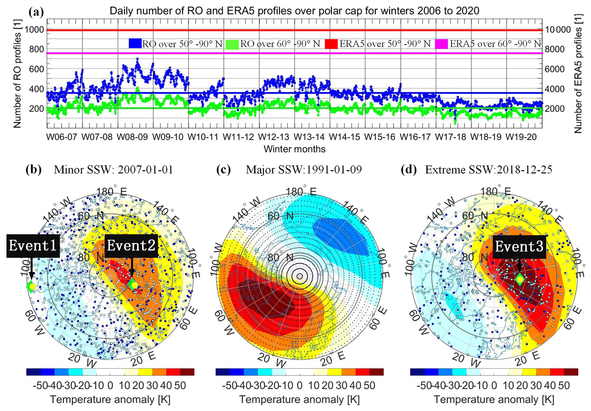
Figure 1Number and distribution of RO and ERA5 profile data over the northern polar region. (a) Daily number of RO events over 50–90∘ N (blue dots) and 60–90∘ N (green dots) for 14 winters from W06–07 to W19–20, with the blue and green horizontal lines showing the related long-term average number, as well as the (constant) daily number of ERA5 grid point profiles (four analysis times per grid point per day; red and magenta lines); (b) illustrative distribution of RO event locations on 1 January 2007 (blue dots) and on the previous and next days (light blue dots) over-plotted on the middle-stratosphere temperature anomaly (MSTA) of the day (color bar), on which a minor SSW prevailed; (c) distribution of the regular ERA5 grid point profile locations (2.5∘ latitude × 2.5∘ longitude grid), over-plotted on the MSTA of 9 January 1991, where a major SSW prevailed; (d) illustrative distribution of RO event locations on 25 December 2018 in the same style as in (b), over-plotted on the MSTA of the day, on which an extreme SSW prevailed. The green diamonds and yellow circles in (b) and (d) show the location of three exemplary RO events and ERA5 profiles (Event1 to Event3) that are located in different SSW anomaly strength conditions and are used in Fig. 2 to illustrate the anomalies construction concept.
Figure 1 illustrates characteristics of the RO and ERA5 profile datasets as relevant for the present SSW study, including the daily number of events available (Fig. 1a) and for exemplary days during SSW events (Fig. 1b–d, see caption for details). Evidently, RO observational atmospheric profile data are comparatively sparse over the (northern high-latitude) region of interest, while ERA5 as a gridded dataset regularly provides its profiles at each and every one of its grid cells without sparsity. Hence, while the number of RO profiles is of the order of several hundred per day, the ones of ERA5 amount to near 10 000 per day. Furthermore, as Fig. 1b–d shows, the spatial distribution of ERA5 data is regular on grid, while RO events occur with reasonable overall coverage but irregular sampling in detail. A few exemplary events (“Event1” to “Event3”) are highlighted, against the back-plot of illustrated SSW temperature anomalies over the polar region, in order to use them next to explain the methodology.
3.3 Methodology
Since we recently provided a detailed basic introduction of the new SSW monitoring approach in Li et al. (2021) and already discussed the main overall features in Sect. 2.2 above, we restrict ourselves to a brief summary here, supported by a schematic overview and concise tabular information and focusing on updates and refinements since that introduction, which provides further technical details.
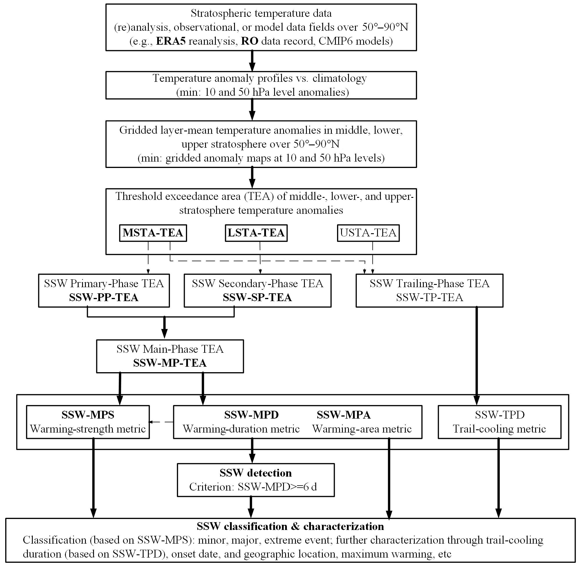
Figure 2Schematic overview of the new SSW detection and monitoring approach and its main algorithmic steps, from the temperature input data (top) to the final SSW metrics (in particular SSW-MPD, SSW-MPA, SSW-MPS; see Table 2, lines 1–3) and their use for detection, classification, and further event characterization (bottom). For implementation details, see Tables 1 and 2 and the description in Sect. 3.3.
As a general overview, Fig. 2 provides a schematic summary of the method's workflow. It highlights the computation sequence, starting with the temperature field input data via anomalies construction and gridded maps generation in stratospheric layers or at pressure levels to extract the threshold exceedance areas (TEAs) of different SSW phases and finally deriving the SSW metrics then used for detection, classification, and characterization. Table 1, which is a condensed and refined update of Table 1 in Li et al. (2021), complements this schematic overview by summarizing the basic parameters and features of the method in more detail along with respective explanations (rightmost column). This ranges from the definition of the temperature anomalies and the related daily TEAs in three characteristic stratospheric layers – lines (1)–(4) – via the anomaly-maximum value and location – lines (5) and (6) – to the four derived TEA key variables during SSW events – lines (7)–(10) – that monitor and characterize the different SSW phases. We note that the daily TEAs for the three layers – lines (2)–(4) – are computed for a range of threshold values for convenient closer insight to the depth of the anomalies (as illustrated in Sect. 4), while only one basic threshold value – boldfaced in lines (2)–(4), middle column – is subsequently used for defining the TEA key variables – lines (7)–(10). All selections and settings summarized and explained in Table 1, including those in the footnotes a–c related to the vertical-resolution options, are based on very extensive sensitivity tests of all the choices, using the ERA5 and RO data as the testing input datasets.
Table 1Basic parameters and methodology of the new SSW monitoring approach – all parameters are updated daily; the boldfaced font in (2)–(4) and (7)–(10) marks key parameters for the monitoring, as also shown in Figs. 7 to 9.
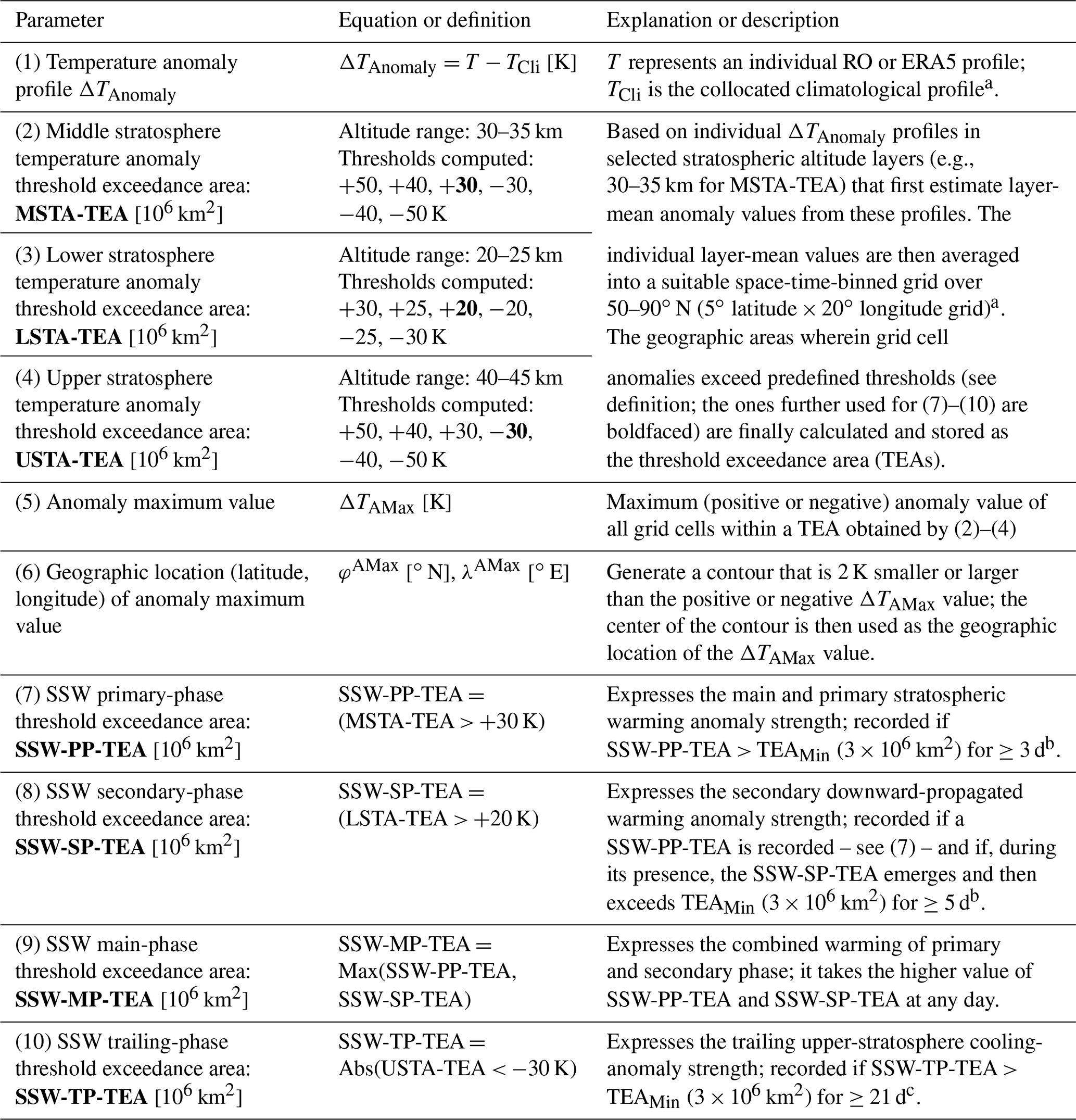
a Regarding the vertical resolution of the (re)analysis, observational, or model simulation input datasets from which the anomaly profiles and layer means are extracted, at least a resolution comparable to the 37 standard pressure level grid of the ERA5 (and other) data is recommended (with a higher vertical resolution preferable, if available). This includes 10 stratospheric-level temperatures from 70 hPa (near 19 km) to 1 hPa (near 48 km), which through simple linear vertical interpolation of temperatures provide adequate profiles for extracting the desired SSW information according to the subsequent steps (2)–(10). Alternatively, as a minimum-input-data approach, temperature map data solely at 10 hPa (∼32 km) and 50 hPa (∼21 km) pressure levels (or similar altitudes) may be used as input, which substitute for the layer-mean values of steps (2) and (3). Step (4) is dropped in this simple two-levels approach, which restricts to middle- and lower-stratospheric TEA data only. b In the simple two-levels approach (see note a), for which the 10 and 50 hPa pressure levels (or corresponding altitudes) are located in the low part of the 5 km layers of the profiles-based approach, TEAMin is set to a reduced value of 2×10⁶ km2 for primary- and secondary-phase TEA. c In addition, in the simple two-levels approach, the MSTA-TEA replaces the USTA-TEA in step (10), and the cooling-anomaly threshold for computing the SSW-TP-TEA is accordingly set to a reduced value of Abs (MSTA-TEA < −20 K).
For aiding the understanding on how the profile and layer-mean anomalies typically look, Fig. 3 graphically illustrates the construction of the anomalies and variables by way of the three example RO events indicated in Fig. 1 and, correspondingly, for three ERA5 profiles from adjacent grid points. It can be seen that RO and ERA5 profiles are overall consistent, with the latter profiles being somewhat smoother in their resolution of vertical variability. Deviations of temperature and corresponding climatological profiles are smallest for Event1 that is located in a non-warming area (see Fig. 1b). Event2 and Event3, which are most affected, show larger deviations and anomalies than Event1, since these are located in the warming area of the SSW (see Fig. 1b and d). The largest anomalies for the latter two events are found in the mid-stratosphere layer (30–35 km), with values of about 45 and 60 K, respectively. Maximum values in the other altitude layers are smaller. In this way, these few examples are consistent with the broader and long-term picture over many SSW events (see Sect. 4 below), which show the SSW warming to be strongest in the middle stratosphere (about 30 to 40 km).

Figure 3Illustration of anomaly construction, layer selection, and computation of layer-mean anomaly values based on the three example RO events and ERA5 profiles indicated in Fig. 1b and d. (a) Event 1 to 3 temperature profiles from RO and collocated climatological profiles ROCli; (b) RO temperature anomaly profiles from the difference of RO to ROCli profiles as well as indication of the lower-stratosphere (20–25 km), middle-stratosphere (30–35 km), and upper-stratosphere (40–45 km) layers and associated layer-mean anomaly values; (c) Profile 1 to 3 temperature and corresponding climatological profiles from ERA5 in same style as (a); (d) ERA5 temperature anomaly profiles and layer-mean values in the same style as (b). The RO satellites and event times and the ERA5 analysis time layers of these examples are as follows (for the locations, see the panel headers): Event1 – COSMIC-FM1 event on 1 January 2007 at 04:28 UTC; Event2 – COSMIC-FM1 event on 1 January 2007 at 22:44 UTC; Event3 – MetOp-A event on 25 December 2018 at 17:04 UTC; Prof1 – ERA5 profile for 1 January 2007 at 06:00 UTC; Prof2 – ERA5 profile for 2 January 2007 at 00:00 UTC; Prof3 – ERA5 profile for 25 December 2018 at 18:00 UTC. The climatological profiles are extracted (and interpolated to the needed locations and times) from long-term-averaged (2006–2020 for RO and 1979–2020 for ERA5) monthly mean temperature fields.
While Li et al. (2021) introduced and initially tested the approach based on the single 2009 SSW event, here we made sure for the long-term application that the four TEA key variables are captured and exploited in such a way that they reliably detect and quantify actual SSW warmings and cooling in the trailing phase, if it occurs, among the ongoing weaker and more “random” polar variability due to other driving factors. The rightmost column of Table 1 – lines (7)–(10) therein – summarizes the criteria that we chose for them after comprehensive testing and sensitivity studies with both the RO and ERA5 data, including on the different options of vertical resolution of the ERA5 temperature input fields. Based on these well-selected TEA key variables and the auxiliary variables on maximum values and locations, all prepared at daily sampling, we could finally define the fundamental metrics and criteria that we use for the detection, classification, and further characterization of SSWs. These definitions were accompanied by another comprehensive portfolio of sensitivity tests, and the choices distilled are summarized in Table 2, including brief explanations (rightmost column therein and footnote *).
Table 2Metrics of the new SSW monitoring approach for detection, classification, and further qualification; the boldfaced font in (1)–(5) marks key metrics and criteria for the detection and classification, also shown as main ones in Fig. 10.
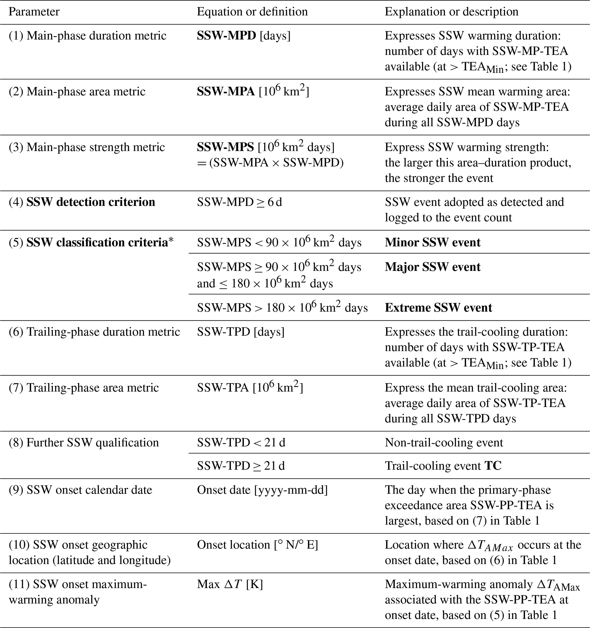
* In the simple two-levels approach (see footnotes a–c of Table 1), where temperature input data solely at 10 and 50 hPa standard pressure levels rather than from vertical profiles are used, the estimated threshold exceedance areas (TEAs) are generally smaller, and hence the SSW-MPS classification boundary values are reduced in this case from 90 and 180×106 km2 days to 70 and 140×106 km2 days, respectively.
Overall, the extensive robustness and sensitivity testing provided us with due evidence and confidence that the new method, effectively constructed from the dynamic temperature anomaly field as perturbed by the SSW, should enable a new level of quality and quantitative insight into SSWs in the long-term, maturing the methodology from our initial Li et al. (2021) single-event study. Hence, as a next step, we applied the method with the parameters and definitions summarized in Table 2 to the complete RO and ERA5 datasets and discuss the results below.
4.1 Polar-cap-mean anomalies overview
Polar cap daily mean temperature anomalies over the 15 winters period from W06–07 to W20–21 are presented in Fig. 4, where both the RO and ERA5 datasets overlap for 14 winters. The RO and ERA5 polar cap results are closely consistent, with anomalies from ERA5 typically about 5 K (occasionally up to 10 K) larger than RO data above 35 km. These differences can mainly be attributed to the denser sampling of ERA5, leading to less spatial smoothing. In general, the overall close results of these independently produced and quite differently sampled datasets (for detailed discussion, see Li et al., 2021) lend confidence that we may use ERA5 data for the inspection of the multi-decadal time period from 1980 onwards.

Figure 4Temporal evolution of polar-cap-mean (60–90∘ N) daily mean temperature anomaly profiles from RO (a) and ERA5 (b) over four winter months each (December, January, February, March) for the winters from 2006–2007 (W06–07) to 2019–2020 for RO (W19–20) and to 2020–2021 for ERA5 (W20–21). The RO dataset did not yet cover the W20–21 time period.
Complementary back-extended polar cap temperature anomalies of ERA5 for the 27 winter periods W79–80 to W05–06 are shown in Fig. 5. The results provide a neat first overview on which winter seasons hosted potentially strong SSWs (e.g., W84–85, W03–04, W18–19) and which were comparatively quiet, including having little evidence of SSWs (e.g., W81–82, W93–94, W10–12). It is also revealed to be a very salient feature already in this polar-cap-mean inspection that strong SSW events often are entailed by a distinct upper-stratospheric cooling, which is hence reflected in our metric definitions – see Table 2, lines (6)–(8). Another interesting feature hinted at here already is that, in the 1990s, where existing SSW climatologies detect very few events (e.g., Charlton and Polvani, 2007; Hu et al., 2015; Butler and Gerber, 2018), we do detect several reasonably strong SSWs that can be classified as major events (more details in Sect. 4.4).
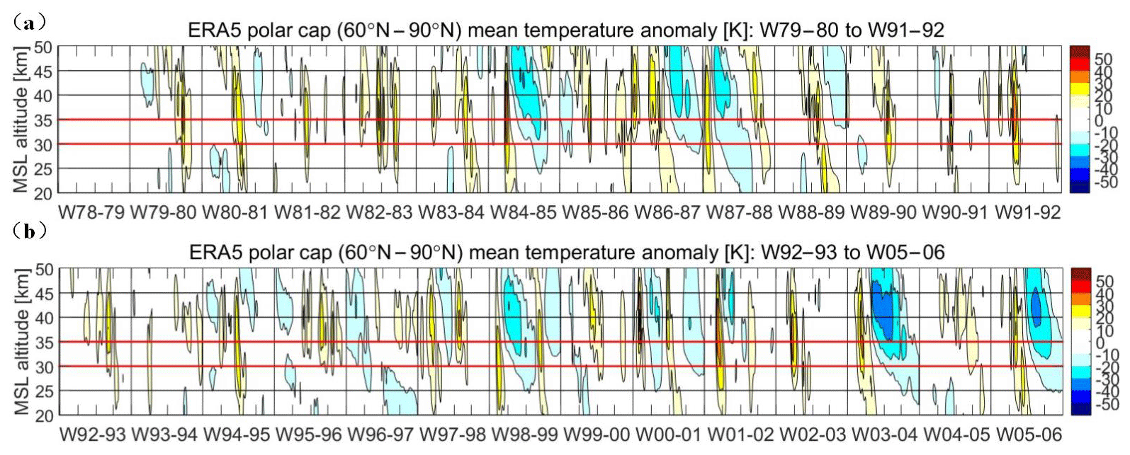
Figure 5Temporal evolution of polar-cap-mean (60–90∘ N) daily mean temperature anomaly profiles from ERA5 over four winter months each (December, January, February, March) for the winters from W79–80 to W91–92 (a) and from W92–93 to W05–06 (b), respectively. The W78–79 time period was not covered by the ERA5 dataset used.
Some distinct temperature anomalies are found in almost every winter in one or another form, which underlines the fact that the polar stratosphere is quite variable in winter. Regarding SSWs, some winters signal one strong warming, while some others show multiple moderately strong or minor warmings. Strong warmings propagate to lower altitude levels and also cause longer-lasting warmings and, as noted above, may be accompanied by distinct cooling (such as in the most recent decade W12–13 and W18–19). A final observation from this basic synoptic view is that the altitude range of maximum warming varies somewhat from event to event. For example, the W11–12 warming is largest at about 35 to 40 km, while the W17–18 warming exhibits its largest anomalies at about 25 to 30 km. Our definition of main phase, combining middle- and lower-stratospheric TEA diagnostics – see Table 1, line (9) – robustly captures such different specific event dynamics.
4.2 Representative results for SSW TEAs
Figure 6 illustrates TEA spatial contour map results for typical daily temperature anomalies across the temporal evolution (top to bottom) of three representative SSW events of increasing strength (left to right; those already used for back-plot in Fig. 1). Evidently, both the temperature anomalies' magnitude and warming area increase from minor to extreme events, as expected based on our classification, which is particularly visible in the mid-stratosphere temperature anomaly on the event onset date (second row). Complementary to this, the snapshot day shown from the trailing phase (four weeks after onset date, bottom row) highlights that the extreme event (right) exhibits a very distinct upper-stratosphere cooling anomaly, exceeding −40 K in a TEA of about 10 million km2 size.
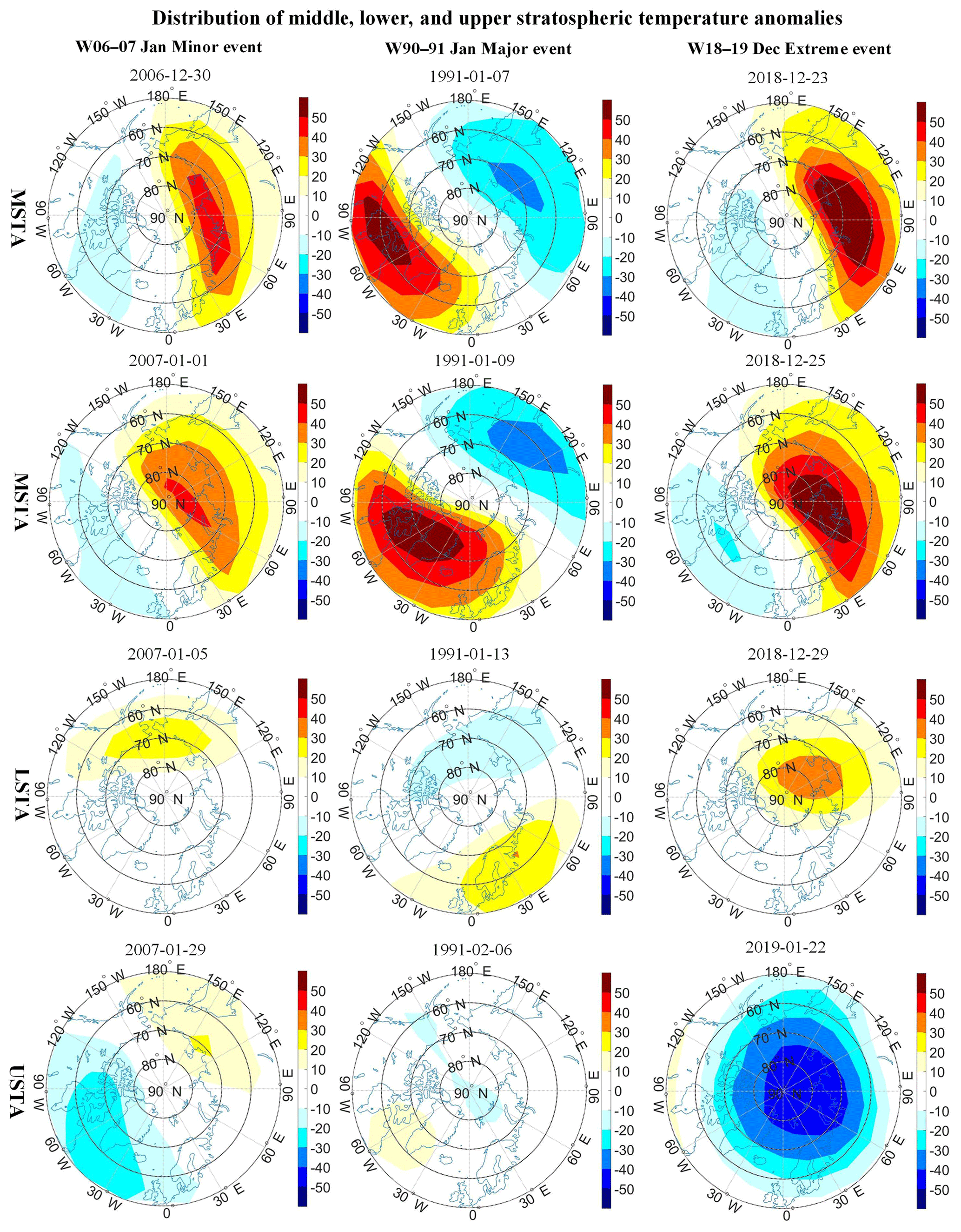
Figure 6Polar-view (50–90∘ N) contour maps of W06–07 January minor (left panels), W90–91 January major (middle), and W18–19 December extreme (right panels) SSW example events (see Figs. 1 and 6), illustrating ERA5-based middle-stratosphere temperature anomalies (MSTAs), lower-stratosphere temperature anomalies (LSTAs), and upper-stratosphere temperature anomalies (USTAs). MSTAs (top and second row panels) are shown 2 d before and on the defined onset date (see Table 2 for definition), LSTAs (third row panels) 4 d after the onset date, and USTAs (bottom panels) 4 weeks after the onset date, respectively.
Following this representative spatial view on individual daily TEAs, Fig. 7 depicts, for the same events as shown in Fig. 6, how our method leads from TEA time series in the three stratospheric layers (first three rows of Fig. 7) to the TEA key variables (fourth row) from which the SSW metrics for the event characterization according to Table 2 are finally derived.
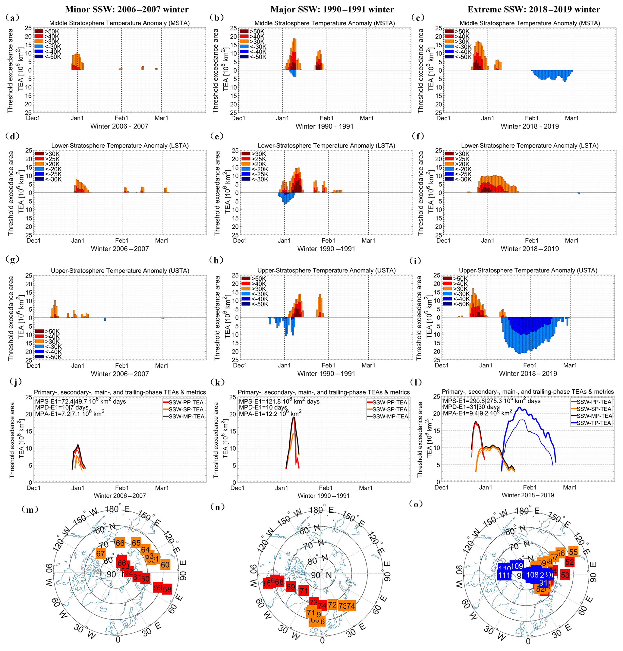
Figure 7Time evolution of the daily ERA5 MSTA (a–c), LSTA (d–f), and USTA (g–i) threshold exceedance areas (TEAs) for the same minor (a, d, g, j, m), major (b, e, h, k, n), and extreme (c, f, i, l, o) SSW events, as illustrated in Fig. 6. Panels (j)–(l) depict the four derived SSW TEAs (SSW-PP-TEA, SSW-SP-TEA, SSW-MP-TEA, and SSW-TP-TEA in case it occurs) according to Table 1, lines (7)–(10); the SSW metrics MPS, MPD, and MPA (see Table 2) are also noted in each panel, and heavy and light lines denote ERA5 and RO results, respectively (difference especially visible for the extreme event). Panels (m)–(o) illustrate geographical tracks (numbered by day of winter as of 1 November) of maximum positive and negative anomaly values of SSW-PP-TEA (red), SSW-SP-TEA (orange), and SSW-TP-TEA (blue).
Daily TEA values over positive thresholds quantify the size of exceedance areas of warming, while those over negative thresholds diagnose the exceedance areas of cooling. It can be seen, for example, that middle-stratosphere temperature anomaly TEAs (MSTA-TEAs) over positive thresholds of all events increase rapidly to maximum and then quickly decrease, indicating the typical sudden warming of the primary phase. Lower-stratosphere temperature anomaly TEAs (LSTA-TEAs) over positive thresholds are overall of smaller magnitude but longer duration, and with maxima delayed against MSTA-TEAs, from the SSW downward propagation. Regarding event strength, while MSTA-TEAs > 30 K of major and extreme events are of small discrepancy within 2×10⁶ km2, the duration of the extreme event is longer than for the major event. The upper-stratosphere temperature anomaly TEA (USTA-TEA) time series of the extreme event shows the distinct several-weeks-long cooling behavior in the trailing phase.
The TEA key variables (Fig. 7j to l) capture the essential daily TEA information per SSW event, in the form summarized in lines (7)–(10) of Table 1, as the basis for the three key metrics per event according to lines (1)–(3) of Table 2, the quantified values of which are shown in the panel legends. As already indicated by the polar-cap-mean view in Figs. 4 and 5, it is well seen here that the ERA5 TEAs (heavy lines) are generally higher than those from the RO data (thin lines), which particularly applies for the trailing-phase cooling of the extreme event (Fig. 7l) in the upper stratosphere, where the sparser sampling by RO events leads to the relatively larger difference. In terms of magnitudes, it is clearly visible from the values that the main-phase strength (MPS), main-phase duration (MPD), and main-phase area (MPA) metrics reach that the event strength grows substantially from minor to extreme – see also the strength class definitions based on the MPS in line (5) of Table 2.
The polar-map plots of Fig. 7 (bottom row) finally illustrate the dynamic event-tracking information of the SSW-PP-TEA, SSW-SP-TEA, and SSW-TP-TEA time series for the three representative events. This view enables one to see the geographic trajectory of the daily anomaly center location – maximum-value location, see line (6) of Table 1 – together with an indication of the anomaly magnitude (color of corresponding TEA thresholds). This type of plot helps the detailed diagnostics and characterization of any specific event, as introduced in Sect. 2 above (for details, see also Li et al., 2021).
4.3 SSW detection and metrics-tracking results
Figures 8 and 9 employ the view introduced in Fig. 7j–l to display the TEA diagnostics and MPS, MPD, and MPA metrics results for all SSWs detected over the full multi-decadal period from 1980 to 2021 (Fig. 8 for the recent winters since 2001–2002 and Fig. 9 for those before, up to 2000–2001). In the recent two decades, typically one or two SSWs occurred during almost every winter (except in W04–05 and W10–11), while in the two decades before, there were somewhat more SSW-quiet winters.
The strongest event during the entire period is the one in W08–09, with a main-phase strength (MPS) of over 360 million km2 days for the ERA5 data (330 million based on the cross-verifying RO data). The second strongest event is the one of W18–19, where the MPS from ERA5 exceeded 290 million km2 days. Additionally, the winters W01–02, W12–13, and W17–18, as well as the winters W84–85, W87–88, and W88–89 in the 1980s, hosted extreme events exceeding our classification threshold of 180×106 km2 days. Half of these eight extreme events also are seen to have caused a strong upper-stratospheric cooling during the trailing phase that lasted for more than a month.
In addition, several major events occurred (e.g., W02–03, W03–04, W05–06), with the MPS of such events varying from 90 to 180×106 km2 days, as defined in Table 2. Also, two of the major events caused a long-lasting upper-stratospheric cooling in the trailing phase (in W03–04 and W05–06); however, this is an exception for these events. Together with these major events, a range of minor events were also detected and diagnosed, exhibiting an MPS smaller than 90×106 km2 days. Based on these long-term SSW tracking results, shown in Figs. 8 and 9, we are now prepared to collect and analyze the long-term results in a more climatological, statistical manner, including inspection for possible long-term transient changes in the record under climate change.
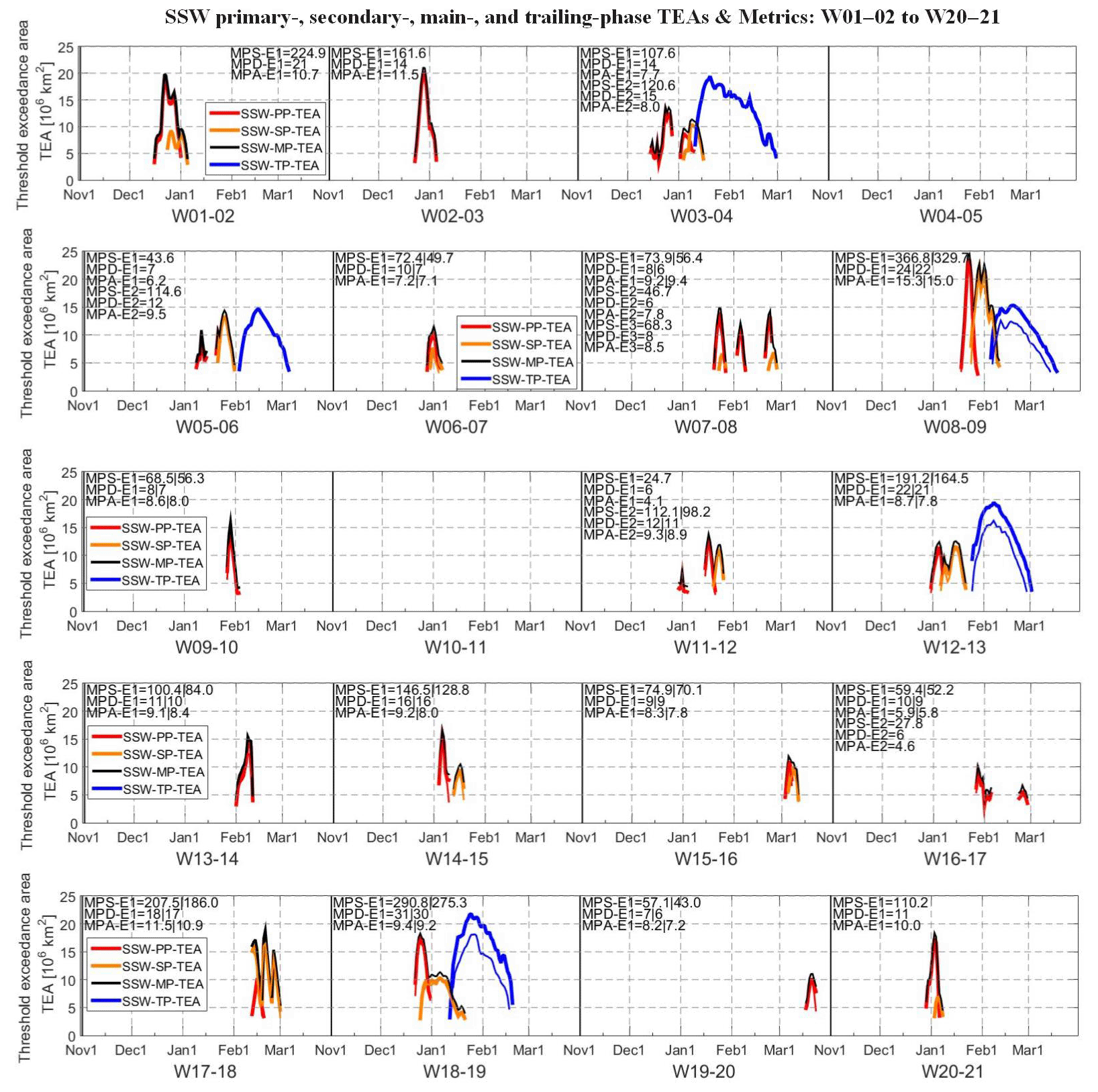
Figure 8Time evolution of the SSW TEAs (SSW-PP-TEA, SSW-SP-TEA, SSW-MP-TEA, SSW-TP-TEA as applicable; for definitions, see Table 1) for all recorded SSW events of the winters W01–02 to W20–21; the SSW metrics MPS, MPD, and MPA (for definitions and units, see Table 2) are noted in the panels (E1, E2, and E3 are SSW event numbers, ordered according to the occurrence time in a winter). ERA5 results (heavy lines) are complemented by RO results (light lines, especially visible for stronger events) for the winters W06–07 to W19–20.
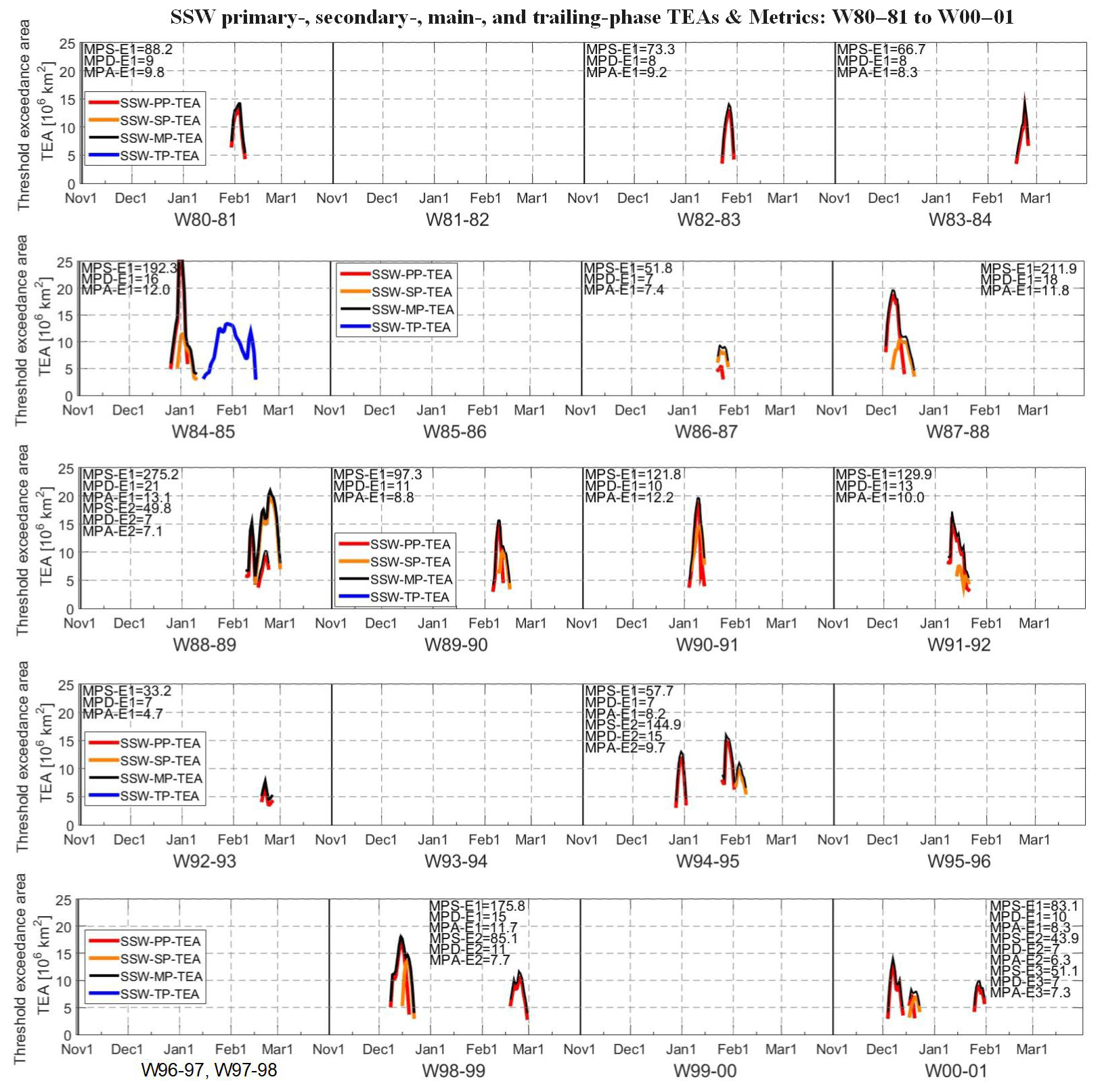
Figure 9Time evolution of the SSW TEAs (SSW-PP-TEA, SSW-SP-TEA, SSW-MP-TEA, SSW-TP-TEA) and related SSW metrics (MPS, MPD, MPA) for all recorded SSW events of the winters W80–81 to W00–01; same plotting style as Fig. 8.
5.1 SSW climatology
Based on the detection results in Sect. 4, a climatological summary of the ERA5-based results for all SSW events detected during the entire 42-year period is provided in Table 3. It lists, for each event, the main characteristics as defined by Table 2 and intercompares the onset dates to the onset dates found by the Butler and Gerber (2018) work (BG18) that extended to the year 2013. The intercomparison reveals that a range of minor and major events was not part of the BG18 list, while several are part of that list and not detected here. In general, the onset dates detected by the new method introduced here are consistent with those in the BG18 climatology, with coincidence of the dates commonly within ±1 d.
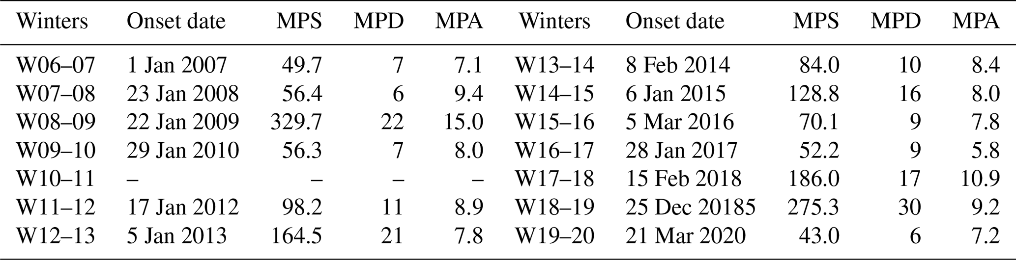
As a complement, the corresponding onset dates and key metrics, as obtained from the RO data, are shown in Table 4. Four minor events (in W07–08, W11–12, and W16–17) did not meet the detection criteria for this dataset, though they were detected based on the ERA5 data. One of the two of W07–08, which overlaps with the BG18 data record, was also not detected by RO data.
In terms of count statistics, 43 events in the 42 winters are detected, corresponding to a frequency of 1.02 per year. This is close to the frequency estimate of 0.9 per year by McInturff (1978). The BG18 climatology, which only lists major SSW events, yields a frequency estimate of 0.6 per year, which is close to the 0.50 per-year frequency we find for our major and extreme events (i.e., discounting the minor events). In general, the high consistency of onset dates with the BG18 definition provides evidence that our new temperature-anomalies-based method is robust in detecting SSW events and that the warming anomalies are strongly related to wind reversals during SSWs. For those events detected by the BG18 definition but not by our method (e.g., the W06–07 event in February 2007), we do find minor warmings also signaled in our TEA diagnostics, but they do not exceed thresholds long enough (for at least 6 d) for detection according to Table 2.
Table 3SSW climatology summary for 1979–2021 based on ERA5 (for definition and units of all parameters, see Table 2; winters where no events are detected by either the new method or the BG18 study are skipped in this list).
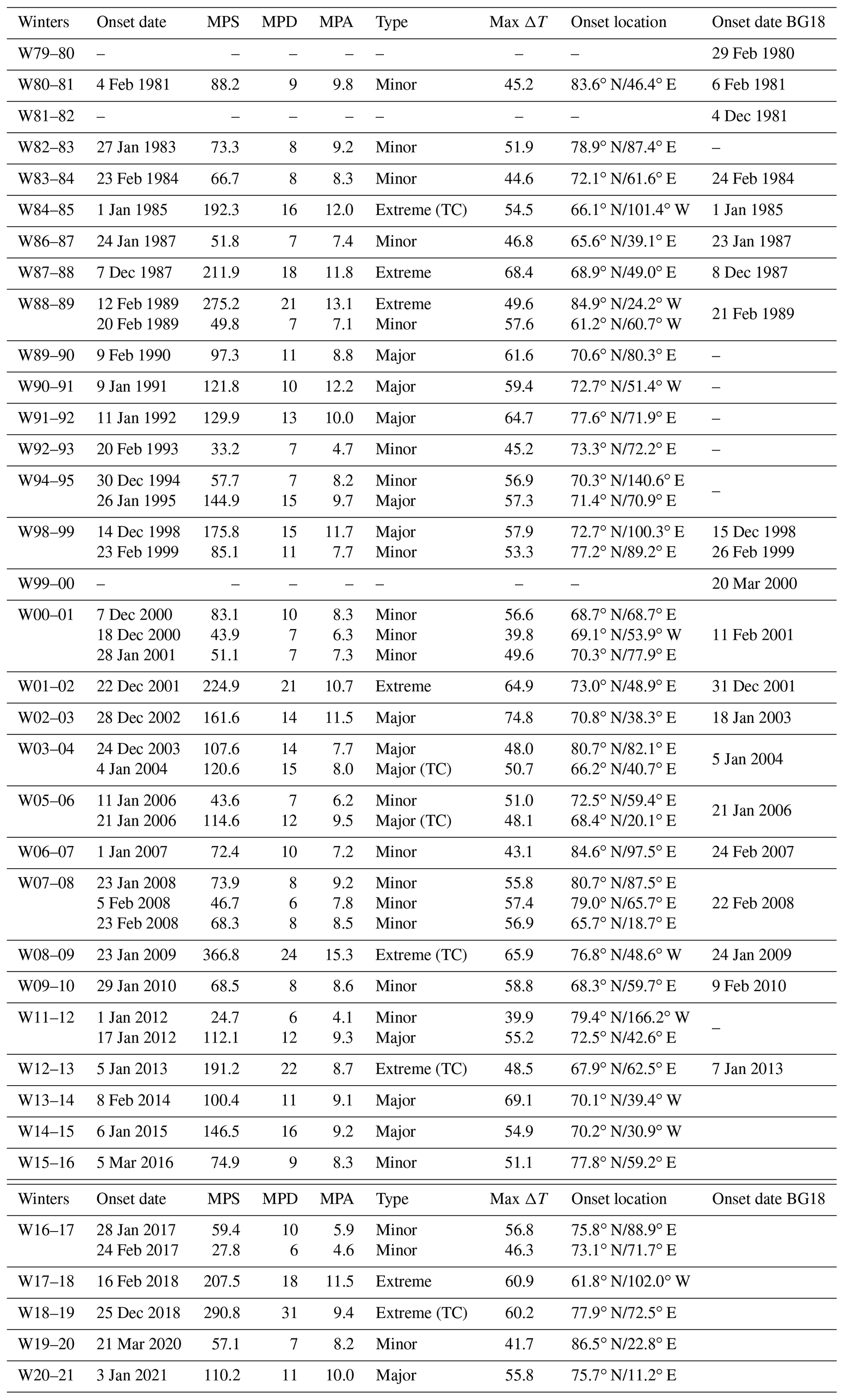
Table 4SSW climatology summary 2006–2020 based on RO for main metrics (left half to W12–13; right half from W13–14), for enabling quantitative intercomparison to the results based on ERA5 as summarized in Table 3 (for definition and units of the parameters, see Table 2).
For the higher number of events detected by us but not detected by the BG18 definition, there are several reasons. The main reason is that a detection based on single altitudes and latitudes misses events occurring in other domains. Related to altitude, we found that a number of events occurred at levels higher than 10 hPa; therefore, such events were not detected by the BG18 definition (e.g., in W92–93 and W00–01). In W07-08, we basically found four warmings (as can be seen in Fig. 4), of which three satisfied our detection criterion. This is in line with Singh and Pallamraju (2015), who also found four warmings based on a temperature increase definition. Related to latitude, Hu et al. (2015) used a wind reversal definition at 65∘ N, detecting an event on 26 January 2010, which is close to our onset date of 29 January 2010 rather than the BG18 date of 9 February 2010. This indicates that selection of a specific latitude for detection also can hinder reliable detection. Finally, some temperature increase events may not be associated with wind reversals at 10 hPa.
Furthermore, we detected a number of events in the 1990s, while BG18 detected only one in W98–99. This can be attributed to three reasons. Firstly, the largest warmings occur at higher altitudes than at the 10 hPa level and therefore may not be detected by data using such a single level. Secondly, a significant amount of radiosonde stations ceased operations in the 1990s, and the availability of wind measurements to the BG18 study for SSW detection was degraded. Thirdly, several warming events are not highly related with wind reversal. Our method, based on temperature data records (here primarily from ERA5, verified by RO data), is robust against such observation network changes, and in addition, temperature is an easily available variable, including in the form of multi-decadal records with reasonable long-term stability.
Figure 10 finally depicts summary statistics on the long-term results along various perspectives of interest, both for the full vertical-resolution (basic case) and coarser-resolution data (see the caption and the respective panel titles for an explanation of the various panels). Regarding the upper half (Fig. 10a–d), it is seen that the results from using the standard pressure level input data (“37-plevels ERA5”) are very similar to those from the basic case (“full-res ERA5”), with the coarser-resolution case detecting only one event less and two events differently. In addition, from simply using linear interpolation between the pressure level temperatures before computing layer-mean temperatures (cf. Fig. 3) from the interpolated coarser-resolution profiles, the SSW strength (MPS) is found to be overall slightly smaller than for the basic case (see the difference of adjacent color and gray symbols in Fig. 10a). However, the size of these differences relative to the basic case is typically smaller than 3 %.
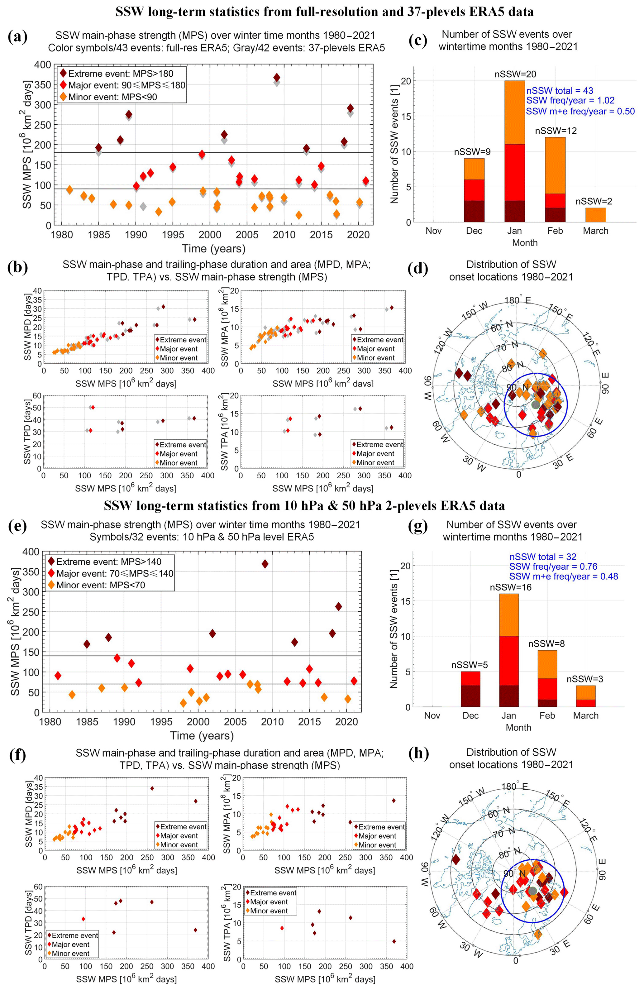
Figure 10Overview of the main characteristics of the SSW events recorded over the 42 winters from 1980 to 2021 using the new monitoring approach based on ERA5 temperature data input at full 137-model-levels resolution (“full-res ERA5”) (upper half, a–d), coarser standard 37-pressure-levels resolution (“37-plevels ERA5”) (co-illustrated in a and b with gray symbols), or simple two-levels data extraction (“10 hPa & 50 hPa level ERA5”) (bottom half, e–h), respectively. (a, e) Time evolution of main-phase strengths (MPS) (year tick marks denote January of year); (b, f) relation of main-phase and trailing-phase duration and area (MPD, MPA; TPD, TPA) to main-phase strength (MPS); (c, g) distribution of the number of events over the winter months (showing the strength types by the same color as in a and e, b and f); (d, h) spatial distribution of onset locations, indicating the clustering of more than 75 % of the events over the northern Eurasia and polar ocean region by a circle (using, again, the same strength-type colors as in a and e, b and f).
Furthermore, while the MPS appears widely variable as a time series (Fig. 10a), the inspection of its component metrics MPD and MPA reveals that the former (the duration) most clearly drives the strength (Fig. 10b, upper left subpanel) and that a salient trail-cooling phase, indicated by the TPD and TPA auxiliary metrics, is dominated by some of the strongest events (Fig. 10b, lower subpanels). Inspecting the SSW onsets, almost all of them (over 95 %) are found within the deep winter (i.e., the December–January–February timeframe, with about half in January; Fig. 10c) and more than three-quarters are found to have their onset location over northern Eurasia and the adjacent polar ocean (Fig. 10d).
The cross-check of using simple two-pressure-levels input data only (“10 hPa & 50 hPa level ERA5”), depicted in the bottom half of Fig. 10e–h, shows that the results are overall similar to the basic case but are notably diluted in the number of detected events (32 instead of 43) and provide systematically smaller MPS estimates by about 20 %–30 % (cf. Fig. 10a and e). The main reason for this is that the downward-propagating warmings are captured at less strength at the 10 hPa (∼32 km) and 50 hPa (∼21 km) levels than by the layer means taken over 30–35 and 20–25 km, respectively. The respective minimum-threshold and MPS classification parameter adjustments for this simple two-levels approach (see Table 1 and 2 footnotes; TEAMin reduced from 3 to 2×10⁶ km2 and classification boundaries lowered from 90–180 to 70–140×106 km2 days) help to compensate for this “low bias” relative to the basic case. The overall detection frequency is nevertheless reduced to 0.76 per year (Fig. 10g), while we find the frequency of the major and extreme events of 0.48 per year to be closely similar to the one for the basic case (0.50 per year). The relative under-detection of events is hence mainly attributable to minor events.
In summary, we thus recommend the use of temperature field data with adequately high vertical resolutions as input to the method. At the same time, the cross-checks demonstrate that the method is also robust and reliable for coarser-resolution data and as a minimum for 10 and 50 hPa level data only, though it is in the latter case somewhat less apt in its detection and monitoring capacity.
5.2 SSW long-term trends
Visually spotting a long-term “tendency” of some possible strength intensification in Fig. 10a and b and the numbers of Table 3, the inspection of long-term trends in the SSW metrics during the climate change period from the 1980s to the 2010s is also of particular interest. Hence, we quantitatively inspected for multi-decadal trends in MPS, MPD, and MPA based on the 33 decadal-mean values of these three metrics over the 1984 to 2016 center years. Regarding a robustness cross-check, we performed this not only for the basic case with full-vertical-resolution input but also for the coarser-resolution cases.
In computing the decadal-mean value of a metric from all individual-event values of a decade, events are allocated to a year based on their onset month, and the mean is obtained from the 10-year-aggregated values over the center year −4 years to the center year +5 years divided by 10 (we also cross-checked to a simple averaging over the events in any 10-year window, which led to similar results but with somewhat more variability due to a direct dependence, in this case, on the sometimes small event count per decade). For the trend fits, we used ordinary-least-squares linear fitting and included uncertainty estimation for the trend rate, accounting for reduced degrees of freedom due to autocorrelation and assuming small-sample t-distribution statistics (Santer et al., 2000; Loeb et al., 2022).
Figure 11 shows that we indeed find a statistically significant positive trend in the MPS, with a best-estimate strength intensification for the basic case (top row, “full-res ERA5”) of about 12(±8) million km2 days per decade (95 % significance level, left subpanel), which is driven by a highly significant increase in the MPD of about 1.8(±0.7) d per decade (99 % significance level, middle subpanel). This implies an increase in the duration of SSW main-phase warmings of about 5(±2) d from the 1980s to the 2010s, raising the average duration by nearly 50 %, from about 10 to 15 d, and inducing an SSW strength increase of about 40(±25) million km2 days, from about 100 to 140 million km2 days.
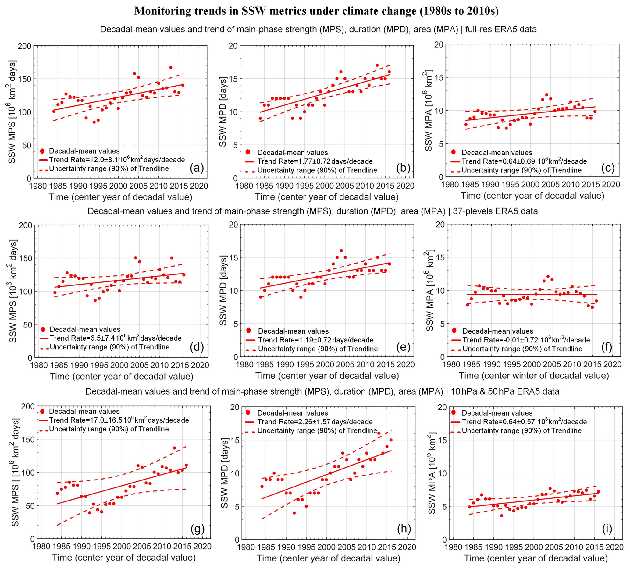
Figure 11Monitoring and assessment of long-term trends in the three core SSW metrics (main-phase strength, duration, and area) along the recent climate change period from the 1980s decade to the 2010s decade, noting also main statistical numbers within the respective panel legends. The results derive from the metrics as illustrated in Fig. 10 and are intercompared for the ERA5 temperature data input either taken in at full 137-model-levels resolution (“full-res ERA5 data”) (a–c), coarser standard 37-pressure-levels resolution (“37-plevels ERA5 data”) (d–f), or simple two-levels data extraction (“10 hPa & 50 hPa ERA5 data”) (g–i), respectively. For a description, see Sect. 5.2.
No robustly significant trend was found in the MPA (right subpanel) or in the associated threshold exceedance magnitude (the average warming strength of the main-phase temperature anomaly above threshold, as indicated by the Max ΔT threshold exceedance defined in line 11 of Table 2), for which sensitivity testing confirmed that it is clearly correlated with the MPA. As part of extensive sensitivity testing, we also found an indication of an increasing trend in the number of major and extreme SSW events of about 0.4 events per decade (near 90 % significance level). The time series is still quite short for such an analysis, however, and it somewhat depends for the minor event counts on the threshold definition for their detection.
The coarser-resolution-based results (middle and bottom row of Fig. 11, “37-plevels ERA5” and “10 hPa & 50 hPa ERA5”) confirm that the trends found are robust across using different input data resolutions (i.e., consistent within the co-estimated uncertainties). Though the mean estimates and associated uncertainty bounds are quite varied across the three cases, reflecting the small-sample statistics with fairly few effective degrees of freedom (typically 8 to 12 only for the 33 decadal-mean values) of the rather short and volatile time series, the overall result of a clearly significant MPD increase that drives a corresponding MPS increase is robustly evident.
While a detailed interpretation and further study of the possible causes of this increase in warming duration, including cross-comparison with other temperature field datasets beyond ERA5, are beyond the scope of this study that focuses on introducing the new monitoring method and related SSW climate data record, we speculate that it may be related to changes in the polar-vortex dynamics over the recent decades that have led to transient changes in prevalent vortex patterns, partly induced by anthropogenic climate change in the polar region (e.g., Kretschmer et al., 2018a, b). Since the MPS metric can be interpreted as an anomalous heat energy content contained in the exceedance warming of an SSW event (similar to the threshold exceedance metric of cooling degree days in the analysis of energy demand during hot days or even heat extremes; Forster et al., 2021), the estimated increase of about 40 % since the 1980s corresponds to substantially more energy stored in and released by recent SSW events.
In this study, we introduced and applied a new method for long-term monitoring of sudden stratospheric warming (SSW) events based on metrics derived from daily stratospheric temperature anomaly threshold exceedance area data, refining the approach introduced in Li et al. (2021), which was based on the well-known 2009 SSW event only. We applied the new method over 1980 to 2021, including 14 winters using radio occultation (RO) data for verification (2006–2020) and all 42 winters within 1980–2021 using ERA5 reanalysis data. Robust SSW characterization metrics, including main-phase duration (MPD), area (MPA), and strength (MPS) are derived, together with further auxiliary diagnostics.
Using these metrics, we proposed a new definition for SSW event detection and classification, and we explored multi-decadal changes in their characteristics under the recent climate change. An SSW is defined to be detected if main-phase warming duration lasts at least 6 d (i.e., SSW-MPD ≥ 6 d). According to MPS, SSWs are classified as minor, major, and extreme events. We also provide an informative SSW climatology over the four decades, recording valuable SSW event characterization information, including onset date, strength, duration, exceedance area, and type of event (minor, major, or extreme), complemented by the maximum-warming-anomaly geographic location and its associated maximum warming. In addition, event trailing-phase metrics as well as day-by-day dynamic tracking of the warming anomaly center location and associated maximum warming and of the areal extent of the exceedance area are available.
Detection results using ERA5 and RO are overall similar, suggesting that the new method can be applied using both ERA5 and RO data as well as any other quality-assured reanalysis, observational, or model temperature (field) data covering the polar region and winter timeframes of interest. Comparison between our climatology and that from the recent BG18 climatology (Butler and Gerber, 2018) reveals that a number of minor and major events were not part of the BG18 study, while several were part of that one and were not detected here. The coincidence of the onset dates of jointly detected events is commonly within ±1 d, suggesting high detection consistency of the different methods and cross-verifying that our new method is robust.
In terms of event count statistics, we detected 43 events in the 42 winters, corresponding to an estimated event frequency of 1.02 per year, close to the event frequency estimate of 0.9 per year by McInturff (1978). Compared to the frequency estimate of 0.6 per year provided by the BG18 study on major SSW events only, the new approach detects about 40 % more events. Within the 1990s, where the BG18 study detected only two in W98–99, we detected seven events (four major and three minor ones). We also found that a salient upper-stratospheric trailing-phase cooling occurs in the wake of the main warming phase for most, though not all, of the strongest events. Regarding temporal and spatial occurrence, we found over 95 % of the SSW onset dates in deep winter (i.e., December–January–February timeframe, with about 50 % in January) and more than three-quarters of the associated onset locations over northern Eurasia and the adjacent polar ocean.
Regarding long-term changes, we found a statistically significant positive trend in the MPS metric, with a best-estimate strength intensification of about 12(±8) million km2 days per decade, which is driven by a highly significant increase in the MPD of about 1.8(±0.7) d per decade. This implies an increase in the duration of SSW main-phase warmings of about 5(±2) d from the 1980s to the 2010s, raising the average duration by nearly 50 %, from about 10 to 15 d, and inducing an SSW strength increase of about 40(±25) million km2 days, from about 100 to 140 million km2 days. These results are found to be robust (i.e., consistent within co-estimated uncertainties) across the use of different vertical resolutions of ERA5 temperature input data. Since the MPS metric can be interpreted as an anomalous heat energy content contained in the exceedance warming of an event, such an increase of about 40 % corresponds to substantially more energy stored in and released by recent SSW events. No robustly significant trend was found in the MPA or in the associated threshold exceedance warming magnitude.
It is hoped that the results of this study can be used as a reference for further complementary and climate-change-related studies and, in particular, also be a basis for SSW impact studies related to other weather and climate phenomena linked to SSWs, such as changes in polar-vortex dynamics and implications to mid-latitude extreme weather. Follow-on work will further investigate the SSWs' long-term evolution over the recent decades and the causes of the evidenced trends. We also intend to investigate whether and how SSW events occurring in different regions have impacts on near-surface weather over middle-latitudinal regions of the Northern Hemisphere.
The code used to produce the results of this study is available from the first author (Ying Li) upon qualified request.
The (numeric) data underlying the results of this study are available from the first author (Ying Li) upon qualified request. The ERA5 reanalysis data are available at full resolution from ECMWF's Mars archive (registered member state users) via https://www.ecmwf.int/en/forecasts/dataset/ecmwf-reanalysis-v5 and publicly at coarser resolution through the Copernicus Climate Change Services (C3S) via https://cds.climate.copernicus.eu/cdsapp#!/dataset/reanalysis-era5-pressure-levels (ECMWF and C3S, 2022). The OPSv5.6 RO data of WEGC are publicly available via https://doi.org/10.25364/WEGC/OPS5.6:2021.1 (EOPAC Team, 2021).
YL implemented and refined the new method, performed the analysis, produced the figures, and wrote the initial draft of the manuscript. GK conceived the method and served as primary co-author, providing advice and guidance on all aspects of the design, analysis, and figure production and significantly contributing to writing the manuscript. MS supported the setup and advancements of the OPS analysis system and provided input data as well as algorithm support. YY advised on analysis and algorithm comparisons. All authors commented on and agreed to the final manuscript.
The contact author has declared that none of the authors has any competing interests.
Publisher's note: Copernicus Publications remains neutral with regard to jurisdictional claims in published maps and institutional affiliations.
We acknowledge ECMWF (Reading, UK) for providing access to their analysis and forecast data and the RO team at WEGC (Graz, Austria) for the preparation of the OPSv5.6 RO data; we specifically acknowledge Florian Ladstädter for supporting RO climatology provision and advising on its characteristics as well as on results interpretation. We furthermore thank the reviewers for their valuable comments that clearly helped to improve the final paper.
The research at the APM (Wuhan, China) was funded by the Strategic Priority Research Program of Chinese Academy of Sciences (grant no. XDA17010304) and the Chinese Natural Sciences Foundation (grant no. 41874040). At WEGC, the work was supported by the Aeronautics and Space Agency of the Austrian Research Promotion Agency (FFG-ALR) under the Austrian Space Applications Programme (ASAP) projects ATROMSAF1 and ATROMSAF2 (project no. 859771 and 873696) funded by the Ministry for Climate, Environment, Energy, Mobility, Innovation, and Technology (BMK).
This paper was edited by Farahnaz Khosrawi and reviewed by Richard Anthes and two anonymous referees.
Angerer, B., Ladstädter, F., Scherllin-Pirscher, B., Schwärz, M., and Kirchengast, G.: Quality aspects of the Wegener Center multi-satellite GPS radio occultation record OPSv5.6, Atmos. Meas. Tech., 10, 4845–4863, https://doi.org/10.5194/amt-10-4845-2017, 2017.
Anthes, R. A.: Exploring Earth's atmosphere with radio occultation: contributions to weather, climate and space weather, Atmos. Meas. Tech., 4, 1077–1103, https://doi.org/10.5194/amt-4-1077-2011, 2011.
Anthes, R. A., Bernhardt, P. A., Chen, Y., Cucurull, L., Dymond, K.F., Ector, D., Healy, S. B., Ho, S. P., Hunt, D. C., Kuo, Y.-H., Liu,H., Manning, K., McCormick, C., Meehan, T. K., Randel, W. J., Rocken, C., Schreiner, W. S., Sokolovskiy, S. V., Syndergaard, S., Thompson, D. C., Trenberth, K. E., Wee, T. K., Yen, N. L., and Zeng, Z.: The COSMIC/FORMOSAT-3 Mission-Early results, B. Am. Meteorol. Soc. 89, 313–333, https://doi.org/10.1175/BAMS-89-3-313, 2008.
Ayarzagüena, B., Langematz, U., Meul, S., Oberländer, S., Abalichin, J., and Kubin, A.: The role of climate change and ozone recovery for the future timing of major stratospheric warmings, Geophys. Res. Lett., 40, 2460–2465, https://doi.org/10.1002/grl.50477, 2013.
Baldwin, M. P. and Thompson, D. W. J.: A critical comparison of stratosphere–troposphere coupling indices, Q. J. Roy. Meteorol. Soc., 135, 1661–1672, https://doi.org/10.1002/qj.479, 2009.
Baldwin, M. P., Ayarzagüena, B., Birner, T., Butchart, N., Butler, A. H., Charlton-Perez, A. J., Domeisen, D. I. V., Garfinkel, C. I., Garny, H., Gerber, E. P., Hegglin, M. I., Langematz, U., and Pedatella, M.: Sudden stratospheric warmings, Rev. Geophys., 59, e2020RG000708, https://doi.org/10.1029/2020RG000708, 2020.
Biondi, R., Steiner, A. K., Kirchengast, G., and Rieckh, T.: Characterization of thermal structure and conditions for overshooting of tropical and extratropical cyclones with GPS radio occultation, Atmos. Chem. Phys., 15, 5181–5193, https://doi.org/10.5194/acp-15-5181-2015, 2015.
Bosilovich, M. G., Kennedy, J., Dee, D., Allan, R., and O'Neill, A.: On the Reprocessing and Reanalysis of Observations for Climate in Climate Science for Serving Society, edited by: Asrar, G. and Hurrell, J., Springer, Dordrecht, https://doi.org/10.1007/978-94-007-6692-1_3, 2013.
Brunner, L., Steiner, A. K., Scherllin-Pirscher, B., and Jury, M. W.: Exploring atmospheric blocking with GPS radio occultation observations, Atmos. Chem. Phys., 16, 4593–4604, https://doi.org/10.5194/acp-16-4593-2016, 2016.
Butler, A. H. and Gerber, E. P.: Optimizing the definition of a sudden stratospheric warming, J. Climate., 31, 2337–2344, https://doi.org/10.1175/JCLI-D-17-0648.1, 2018.
Butler, A. H., Seidel, D. J., Hardiman, S. C., Butchart, N., Birner, T., and Match, A.: Defining sudden stratospheric warmings, B. Am. Meteorol. Soc., 96, 1913–1928, https://doi.org/10.1175/BAMS-D-13-00173.1, 2015.
Butler, A. H., Sjoberg, J. P., Seidel, D. J., and Rosenlof, K. H.: A sudden stratospheric warming compendium, Earth Syst. Sci. Data, 9, 63–76, https://doi.org/10.5194/essd-9-63-2017, 2017.
Cattiaux, J. R., Vautard, R., Cassou, C., Yiou, P., and Codron, F.: Winter 2010 in Europe: a cold extreme in a warming climate, Geophys. Res. Lett., 37, 114–122, https://doi.org/10.1029/2010GL044613, 2010.
Charlton, A. J. and Polvani, L. M.: A new look at stratospheric sudden warmings: Part I: Climatology and modeling benchmarks, J. Climate., 20, 449–469, https://doi.org/10.1175/JCLI3996.1, 2007.
Dee, D. P., Uppala, S. M., Simmons, A. J., Berrisford, P., Poli, P., Kobayashi, S., Andrae, U., Balmaseda, M. A., Balsamo, G., Bauer, P., Bechtold, P., Beljaars, A. C. M., van de Berg, L., Bidlot, J., Bormann, N., Delsol, C., Dragani, R., Fuentes, M., Geer, A. J., Haimberger, L., Healy, S. B., Hersbacha, H., Hólm, E. V., Isaksena, L., Kållberg, P., Köhler, M., Matricardi, M., McNally, A. P., Monge-Sanz, B. M., Morcrette, J.-J., Park, B.-K., Peubey, C., de Rosnay, P., Tavolato, C., Thépaut J.-N., and Vitart, F.: The ERA-Interim reanalysis: Configuration and performance of the data assimilation system, Q. J. Roy. Meteorol. Soc., 137, 553–597, https://doi.org/10.1002/qj.828, 2011.
Dhaka, S. K., Kumar, V., Choudhary, R. K., Ho, S. P., Takahashi, M., and Yoden, S.: Indications of a strong dynamical coupling between the polar and tropical regions during the sudden stratospheric warming event January 2009, based on COSMIC/FORMASAT-3 satellite temperature data, Atmos. Res., 166, 60–69, https://doi.org/10.1016/j.atmosres.2015.06.008, 2015.
ECMWF and C3S: ERA5 reanalysis data, European Centre for Medium-Range Weather Forecasts (ECMWF) and Copernicus Climate Change Service (C3S), Reading, UK, ECMWF and C3S [data set], https://www.ecmwf.int/en/forecasts/dataset/ecmwf-reanalysis-v5 (full resolution; registered ECMWF member state users), https://cds.climate.copernicus.eu/cdsapp#!/dataset/reanalysis-era5-pressure-levels (coarse resolution; general C3S users), last access: 15 June 2022.
EOPAC Team: GNSS Radio Occultation Record (OPS 5.6 2001–2020), Wegener Center, University of Graz, Graz, Austria, EOPAC Team [data set], https://doi.org/10.25364/WEGC/OPS5.6:2021.1, 2021.
Foelsche, U., Scherllin-Pirscher, B., Ladstädter, F., Steiner, A. K., and Kirchengast, G.: Refractivity and temperature climate records from multiple radio occultation satellites consistent within 0.05 %, Atmos. Meas. Tech., 4, 2007–2018, https://doi.org/10.5194/amt-4-2007-2011, 2011.
Forster, P., Storelvmo, T., Armour, K., Collins, W., Dufresne, J.-L., Frame, D., Lunt, D. J., Mauritsen, T., Palmer, M. D., Watanabe, M., Wild, M., and Zhang, H.: The Earth's energy budget, climate feedbacks, and climate sensitivity (Chapter 7), in: Climate Change 2021: The Physical Science Basis, Contribution of Working Group I to the Sixth Assessment Report of the Intergovernmental Panel on Climate Change, edited by: Masson-Delmotte, V., Zhai, P., Pirani, A., Connors, S. L., Pean, S., Berger, N., Caud, Y., Chen, L., Goldfarb, M. I., Gomis, M., Huang, K., Leitzell, E., Lonnoy, J. B. R., Matthews, T. K., Maycock, C., Waterfield, T., Yelekci, O., Yu, R., and Zhou, B., Cambridge University Press, Cambridge, UK and New York, NY, USA, 923–1054, https://www.ipcc.ch/report/ar6/wg1/chapter/chapter-7/ (last access: 17 January 2023), 2021.
Garfinkel, C. I., Silverman, V., Harnik, N., Haspel, C., and Riz, Y.: Stratospheric response to intraseasonal changes in incoming solar radiation, J. Geophys.Res. Atmos., 120, 7648–7660, https://doi.org/10.1002/2015JD023244, 2015.
Gerber, E. P., Baldwin, M. P., Akiyoshi, H., Austin, J., and Dan, S.: Stratosphere-troposphere coupling and annular mode variability in chemistry-climate models, J. Geophys. Res., 115, D00M06, https://doi.org/10.1029/2009JD013770, 2010.
Gobiet, A., Kirchengast, G., Manney, G. L., Borsche, M., Retscher, C., and Stiller, G.: Retrieval of temperature profiles from CHAMP for climate monitoring: intercomparison with Envisat MIPAS and GOMOS and different atmospheric analyses, Atmos. Chem. Phys., 7, 3519–3536, https://doi.org/10.5194/acp-7-3519-2007, 2007.
Hall, R. J., Mitchell, D. M., Seviour, W. J. M., and Wright, C. J.: Tracking the stratosphere-to-surface impact of Sudden Stratospheric Warmings, J. Geophys. Res.-Atmos., 126, e2020JD033881, https://doi.org/10.1029/2020JD033881, 2021.
Hersbach, H., Bell, W., Berrisford, P., Horányi, A., Muñoz-Sabater, J., Nicolas, J., Radu, R., Schepers., D, Simmons, A., Soci, C., and Dee, D.: Global reanalysis: goodbye ERA-Interim, hello ERA5, ECMWF Newslett., 159, 17–24, https://doi.org/10.21957/vf291hehd7, 2019.
Hersbach, H., Bell, B., Berrisford, P., Hirahara, S., Horányi1, A., Muñoz-Sabater, J., Nicolas, J., Peubey, C., Radu, R., Schepers, D., Simmons, A., Soci, C., Abdalla, S., Abellan, X., Balsamo, G., Bechtold, P., Biavati, G., Bidlot, J., Bonavita, M., De Chiara1, G., Dahlgren, P., Dee, D., Diamantakis, M., Dragani, R., Flemming, J., Forbes, R., Fuentes, M., Geer, A., Haimberger, L., Healy, S., Hogan1,R.J., Hólm, E., Janisková, M., Keeley, S., Laloyaux, P., Lopez, P., Radnoti, G., De Rosnay, P., Rozum, I., Vamborg, F., Villaume, S., and Thépaut. J.-N.: The ERA5 global reanalysis, Q. J. Roy. Meteorol. Soc., 146, 1999–2049, https://doi.org/10.1002/qj.3803, 2020.
Hitchcock, P. and Shepherd, T. G.: Zonal-mean dynamics of extended recoveries from stratospheric sudden warmings, J. Atmos. Sci., 70, 688–707, https://doi.org/10.1175/JAS-D-12-0111.1, 2013.
Hitchcock, P. and Simpson, I. R.: The downward influence of stratospheric sudden warmings, J. Atmos. Sci., 71, 3586–3876, https://doi.org/10.1175/JAS-D-14-0012.1, 2014.
Holt, L. A., Randall, C. E., Peck, E. D., Marsh, D. R., Smith, A. K., and Harvey, V. L.: The influence of major sudden stratospheric warming and elevated stratopause events on the effects of energetic particle precipitation in WACCM, J. Geophys. Res.-Atmos., 118, 11636–11646, https://doi.org/10.1002/2013JD020294, 2013.
Hu, J., Ren, R., and Xu, H.: Occurrence of winter stratospheric sudden warming events and the seasonal timing of spring stratospheric final warming, J. Atmos. Sci.,71, 2319–2334, https://doi.org/10.1175/JAS-D-13-0349.1, 2015.
Johnson, K. W., Miller, A. J., and Gelman, M.: Proposed indices characterizing stratospheric circulation and temperature fields, Mon. Weather Rev., 97, 565–570, https://doi.org/10.1175/1520-0493(1969)097<0565:PICSCA>2.3.CO;2, 1969.
Jonah, O. F., de Paula, E. R., Kherani, E. A., Dutra, S. L. G., and Paes, R. R.: Atmospheric and ionospheric response to sudden stratospheric warming of January 2013, J. Geophys. Res.-Space, 119, 4973–4980, https://doi.org/10.1002/2013JA019491, 2014.
Kakoti, G., Kalita, B. R., Bhuyan, P. K., Baruah, S., and Wang, K.: Longitudinal and interhemispheric ionospheric response to 2009 and 2013 SSW events in the African-European and Indian-East Asian sectors, J. Geophys. Res.-Space, 125, e2020JA028570, https://doi.org/10.1029/2020JA028570, 2020.
Kirchengast, G.: Occultations for probing atmosphere and climate: Setting the scene, in: Occultations for Probing Atmosphere and Climate, edited by: Kirchengast, G., Foelsche, U., and Steiner, A. K., Springer, Berlin, Heidelberg, 1–8, https://doi.org/10.1007/978-3-662-09041-1_1, 2004.
Klingler, R.: Observing Sudden Stratospheric Warmings with Radio Occultation Data, with Focus on the Event 2009, MSc Thesis, University of Graz, Graz, Austria, 85 pp., https://resolver.obvsg.at/urn:nbn:at:at-ubg:1-68069 (last access: 15 June 2022), 2014.
Kretschmer, M., Coumou, D., Agel, L., Barlow, M., Tziperman, E., and Cohen, J.: More-persistent weak stratospheric polar vortex states linked to cold extremes, B. Am. Meteorol. Soc., 99, 49–60, https://doi.org/10.1175/BAMS-D-16-0259.1, 2018a.
Kretschmer, M., Cohen, J., Matthias, V., Runge, J., and Coumou, D.: The different stratospheric influence on cold-extremes in Eurasia and North America, Clim. Atmos. Sci., 1, 44, https://doi.org/10.1038/s41612-018-0054-4, 2018b.
Kursinski, E. R., Hajj, G. A., Schofield, J. T., Linfield, R. P., and Hardy, K. R.: Observing Earth's atmosphere with radio occultation measurements using the Global Positioning System, J. Geophys. Res., 102, 23429–23465, https://doi.org/10.1029/97JD01569, 1997.
Kuttippurath, J. and Nikulin, G.: A comparative study of the major sudden stratospheric warmings in the Arctic winters 2003/2004–2009/2010, Atmos. Chem. Phys., 12, 8115–8129, https://doi.org/10.5194/acp-12-8115-2012, 2012.
Labitzke, K.: Stratospheric-mesospheric midwinter disturbances: A summary of observed characteristics, J. Geophys. Res., 86, 9665–9678, https://doi.org/10.1029/JC086iC10p09665, 1981.
Labitzke, K. and Kunze, M.: On the remarkable Arctic winter in 2008/2009, J. Geophys. Res.-Atmos., 114, D00I02, https://doi.org/10.1029/2009JD012273, 2009.
Ladstädter, F., Steiner, A. K., Schwärz, M., and Kirchengast, G.: Climate intercomparison of GPS radio occultation, RS90/92 radiosondes and GRUAN from 2002 to 2013, Atmos. Meas. Tech., 8, 4, 1819–1834, https://doi.org/10.5194/amt-8-1819-2015, 2015.
Lehtonen, I. and Karpechko, A. Y.: Observed and modeled tropospheric cold anomalies associated with sudden stratospheric warmings, J. Geophys. Res.-Atmos., 121, 1591–1610, https://doi.org/10.1002/2015JD023860, 2016.
Li, Y., Kirchengast, G., Schwaerz, M., Ladstädter, F., and Yuan, Y.-B.: Monitoring Sudden Stratospheric Warmings using radio occultation: a new approach demonstrated based on the 2009 event, Atmos. Meas. Tech., 14, 2327–2343, https://doi.org/10.5194/amt-14-2327-2021, 2021.
Lin, J. T., Lin, C. H., Chang, L.C., Huang, H. H., Liu, J. Y., Chen, A. B., Chen, C. H., and Liu, C. H.: Observational evidence of ionospheric migrating tide modification during the 2009 stratospheric sudden warming, Geophys. Res. Lett., 39, L02101, https://doi.org/10.1029/2011GL050248, 2012.
Loeb, N. G., Mayer, M., Kato, S., Fasullo, J. T., Zuo, H., Senan, R., Lyman, J. M., Johnson, G. C., and Balmaseda, M.: Evaluating Twenty-Year Trends in Earth’s Energy Flows From observations and reanalyses, J. Geophys. Res.-Atmos., 127, e2022JD036686, https://doi.org/10.1029/2022JD036686, 2022.
Luntama, J.-P., Kirchengast, G., Borsche, M., Foelsche, U., Steiner, A., Healy, S., von Engeln, A., O'Clerigh, E., and Marquardt, C.: Prospects of the EPS GRAS mission for operational atmospheric applications, B. Am. Meteorol. Soc., 89, 1863–1875, https://doi.org/10.1175/2008BAMS2399.1, 2008.
Manney, G. L., Lawrence, Z. D., Santee, M. L., Read, W. G., Livesey, N. J., Lambert, A., Froidevaux, L., Pumphrey, H. C., and Schwartz M. J.: A minor sudden stratospheric warming with a major impact: Transport and polar processing in the 2014/2015 Arctic winter, Geophys. Res. Lett., 42, 7808–7816, https://doi.org/10.1002/2015GL065864, 2015.
McInturff, R. M.: Stratospheric warmings: Synoptic, dynamic and general-circulation aspects, NASA Reference Publ., NASA-RP-1017, NASA, USA, 174 pp., https://ntrs.nasa.gov/archive/nasa/casi.ntrs.nasa.gov/19780010687.pdf (last access: 15 June 2022), 1978.
Mitchell, D. M., Gray, L. J.,Anstey, J., Baldwin, M. P., and Charlton-Perez A. J.: The influence of stratospheric vortex displacements and splits on surface climate, J. Climate, 26, 2668–2682, https://doi.org/10.1175/JCLI-D-12-00030.1, 2013.
Nayak, C. and Yigit, E.: Variation of small-scale gravity wave activity in the ionosphere during the major sudden stratospheric warming event of 2009, J. Geophys. Res.-Space, 124, 470–488, https://doi.org/10.1029/2018JA026048, 2019.
Noguchi, S., Kuroda, Y., Mukougawa, H., Mizuta, R., and Kobayashi, C.: Impact of satellite observations on forecasting sudden stratospheric warmings, Geophys. Res. Lett., 47, e2019GL086233, https://doi.org/10.1029/2019GL086233, 2020.
Parker, W. S.: Reanalyses and observations: What's the difference, B. Am. Meteorol. Soc., 97, 1565–1572, https://doi.org/10.1175/BAMS-D-14-00226.1, 2016.
Santer, B. D., Wigley, T., Boyle, J. S., Gaffen, D. J., Hnilo, J. J., and Nychka, D.: Statistical significance of trends and trend differences in layer-average atmospheric temperature time series, J. Geophys. Res., 105, 7337–7356, https://doi.org/10.1029/1999jd901105, 2000.
Scherhag, R.: Die explosionsartige Stratosphärenerwärmung des Spätwinters 1951/52, Ber. Deut. Wetterdienst, 38, 51–63, 1952.
Scherllin-Pirscher, B., Kirchengast, G., Steiner, A. K., Kuo, Y.-H., and Foelsche, U.: Quantifying uncertainty in climatological fields from GPS radio occultation: an empirical-analytical error model, Atmos. Meas. Tech., 4, 2019–2034, https://doi.org/10.5194/amt-4-2019-2011, 2011a.
Scherllin-Pirscher, B., Steiner, A. K., Kirchengast, G., Kuo, Y.-H., and Foelsche, U.: Empirical analysis and modelling of errors of atmospheric profiles from GPS radio occultation, Atmos. Meas. Tech., 4, 1875–1890, https://doi.org/10.5194/amt-4-1875-2011, 2011b.
Scherllin-Pirscher, B., Steiner, A. K., Kirchengast, G., Schwaerz, M., and Leroy, S. S.: The power of vertical geolocation of atmospheric profiles from GNSS radio occultation, J. Geophys. Res.-Atmos., 122, 1595–1616, https://doi.org/10.1002/2016JD025902, 2017.
Schoeberl, M. R.: Stratospheric warmings: Observations and theory, Rev. Geophys., 16, 521–538, https://doi.org/10.1029/RG016i004p00521, 1978.
Schreiner, W., Rocken, C., Sokolovskiy, S., Syndergaard, S., and Hunt, D.: Estimates of the precision of GPS radio occultations from the COSMIC/FORMOSAT-3 mission, Geophys. Res. Lett., 34, L04808, https://doi.org/10.1029/2006GL027557, 2007.
Schwärz, M., Kirchengast, G., Scherllin-Pirscher, B., Schwarz, J., Ladstädter, F., and Angerer, B.: Multi-mission validation by satellite radio occultation extension project–Final report, Tech. Rep. for ESA/ESRIN No. 01/2016, Wegener Center, University of Graz, Graz, Austria, https://wegcwww.uni-graz.at/publ/wegcpubl/arsclisys/2016/Schwaerz-etal_MMValRO-FinRep_Dec2016.pdf (last access: 12 December 2021), 2016
Seviour, W. J. M., Mitchell, D. M., and Gray, L. J.: A practical method to identify displaced and split stratospheric polar vortex events, Geophys. Res. Lett., 40, 5268–5273, https://doi.org/10.1002/grl.50927, 2013.
Simmons, A., Soci, C., Nicolas, J., Bell, B., Berrisford, P., Dragani, R., Flemming, J., Haimberger1, L., Healy, S., Hersbach, H., Horányi, A., Inness, A., Muñoz-Sabater, J., Radu, R., and Schepers, D.: Global stratospheric temperature bias and other stratospheric aspects of ERA5 and ERA5.1, ECMWF Tech. Memo. No. 859, ECMWF, https://doi.org/10.21957/rcxqfmg0, 2020.
Singh, R. P. and Pallamraju, D.: On the latitudinal distribution of mesospheric temperatures during sudden stratospheric warming events, J. Geophys. Res.-Space, 120, 2926–2939, https://doi.org/10.1002/2014JA020355, 2015.
Siskind, D. E., Eckermann, S. D., McCormack, J. P., Coy, L., Hoppel, K. W., and Baker, N. L.: Case studies of the mesospheric response to recent minor, major, and extended stratospheric warmings, J. Geophys. Res., 115, D00N03, https://doi.org/10.1029/2010JD014114, 2010.
Steiner, A. K., Lackner, B. C., Ladstädter, F., Scherllin-Pirscher, B., Foelsche, U., and Kirchengast, G.: GPS radio occultation for climate monitoring and change detection, Radio Sci., 46, RS0D24, https://doi.org/10.1029/2010RS004614, 2011.
Steiner, A. K., Ladstädter, F., Ao, C. O., Gleisner, H., Ho, S.-P., Hunt, D., Schmidt, T., Foelsche, U., Kirchengast, G., Kuo, Y.-H., Lauritsen, K. B., Mannucci, A. J., Nielsen, J. K., Schreiner, W., Schwärz, M., Sokolovskiy, S., Syndergaard, S., and Wickert, J.: Consistency and structural uncertainty of multi-mission GPS radio occultation records, Atmos. Meas. Tech., 13, 2547–2575, https://doi.org/10.5194/amt-13-2547-2020, 2020a.
Steiner, A. K., Ladstädter, F., Randel, W. J., Maycock, A. C., Fu, Q., Claud, C., Gleisner, H., Haimberger, L., Ho, S.-P., Keckhut, P., Leblanc, T., Mears, C., Polvani, L. M., Santer, B. D., Schmidt, T., Sofieva, V., Wing, R., and Zou, C.-Z.: Observed temperature changes in the troposphere and stratosphere from 1979 to 2018, J. Climate., 33, 8165–8194, https://doi.org/10.1175/JCLI-D-19-0998.1, 2020b.
Stocker, M., Ladstädter, F., and Steiner, A. K.: Observing the climate impact of large wildfires on stratospheric temperature, Sci. Rep., 11, 22994, https://doi.org/10.1038/s41598-021-02335-7, 2021.
Sun, Y., Bai, W., Liu, C., Liu, Y., Du, Q., Wang, X., Yang, G., Liao, M., Yang, Z., Zhang, X., Meng, X., Zhao, D., Xia, J., Cai, Y., and Kirchengast, G.: The FengYun-3C radio occultation sounder GNOS: a review of the mission and its early results and science applications, Atmos. Meas. Tech., 11, 5797–5811, https://doi.org/10.5194/amt-11-5797-2018, 2018.
Thompson, D. W. J., Baldwin, M. P., and Wallace, J. M.: Stratospheric connection to northern hemisphere wintertime weather: implications for prediction, J. Climate, 15, 1421–1428, https://doi.org/10.1175/1520-0442(2002)015<1421:SCTNHW>2.0.CO;2, 2002.
Tyrlis, E., Manzini, E., Bader, J., Ukita, J., Nakamura, H., and Matei, D.: Ural blocking driving extreme Arctic sea ice loss, cold Eurasia, and stratospheric vortex weakening in autumn and early winter 2016–2017, J. Geophys. Res.-Atmos., 124, 11313–11329, https://doi.org/10.1029/2019JD031085, 2019.
Van Loon, H., Jenne, R. L., and Labitzke, K.: Zonal harmonic standing waves, J. Geophys. Res., 78, 4463–4471, https://doi.org/10.1029/JC078i021p04463, 1973.
Vignon, E. and Mitchell, D. M.: The stratopause evolution during different types of sudden stratospheric warming event, Clim. Dynam., 44, 3323–3337, https://doi.org/10.1007/s00382-014-2292-4, 2015.
Wickert, J., Reigber, C., Beyerle, G., König, R., Marquardt, C., Schmidt, T., Grundwaldt, L., Galas, R., Meehan, T. K., Melbourne, W. G., and Hocke, K.: Atmosphere sounding by GPS radio occultation: First results from CHAMP, Geophys. Res. Lett., 28, 3263–3266, https://doi.org/10.1029/2001GL013117, 2001.
Wickert, J., Beyerle, G., König, R., Heise, S., Grunwaldt, L., Michalak, G., Reigber, C., and Schmidt, T.: GPS radio occultation with CHAMP and GRACE: A first look at a new and promising satellite configuration for global atmospheric sounding, Ann. Geophys., 23, 653–658, https://doi.org/10.5194/angeo-23-653-2005, 2005.
WMO/IQSY.: International Years of the Quiet Sun (IQSY), 1964–1965: Alert messages with special references to stratwarms, Secretariat of the WMO WMO/IQSY Rep. 6, 19 pp., 1964.
Yoshida, K. and Yamazaki, K.: Tropical cooling in the case of stratospheric sudden warming in January 2009: focus on the tropical tropopause layer, Atmos. Chem. Phys., 11, 6325–6336, https://doi.org/10.5194/acp-11-6325-2011, 2011.
Yu, Y., Ren, R., and Cai, M.: Dynamic linkage between cold air outbreaks and intensity variations of the meridional mass circulation, J. Atmos. Sci., 72, 3214–3232, https://doi.org/10.1175/JAS-D-14-0390.1, 2015.
Yue, X., Schreiner, W. S., Lei, J., Rocken, C., Hunt, D. C., Kuo, Y.-H., and Wan, W.: Global ionospheric response observed by COSMIC satellites during the January 2009 stratospheric sudden warming event, J. Geophys. Res., 115, A00G09, https://doi.org/10.1029/2010JA015466, 2010.
Zhou, S., Miller, A. J., Wang, J., and Angell, J. K.: Downward-propagating temperature anomalies in the preconditioned polar stratosphere, J. Climate, 15, 781–792, https://doi.org/10.1175/1520-0442(2002)015<0781:DPTAIT>2.0.CO;2, 2002.
- Abstract
- Introduction
- Assessment of current definitions and the new method
- Data and methodology
- SSW detection and monitoring results
- SSW climatology and trends under climate change
- Conclusions
- Code availability
- Data availability
- Author contributions
- Competing interests
- Disclaimer
- Acknowledgements
- Financial support
- Review statement
- References