Development and evaluation of processes affecting simulation of diel fine particulate matter variation in the GEOS-Chem model

The capability of chemical transport models to represent fine particulate matter (PM_2.5) over the course of a day is of vital importance for air quality simulation and assessment. In this work, we used the nested GEOS-Chem model at $\mathrm{0.25}{}^{\circ }\times \mathrm{0.3125}{}^{\circ }$ resolution to simulate the diel (24 h) variation in PM_2.5 mass concentrations over the contiguous United States (US) in 2016. We evaluate the simulations with in situ measurements from a national monitoring network. Our base case simulation broadly reproduces the observed morning peak, afternoon dip, and evening peak of PM_2.5, matching the timings of these features within 1–3 h. However, the simulated PM_2.5 diel amplitude in our base case was 106 % biased high, relative to observations. We find that temporal resolution of emissions, subgrid vertical gradient between surface model-level center and observations, and biases in boundary layer mixing and aerosol nitrate are the major causes for this inconsistency. We applied an hourly anthropogenic emission inventory, converted the PM_2.5 mass concentrations from the model-level center to the height of surface measurements by correcting for aerodynamic resistance, adjusted the boundary layer heights in the driving meteorological fields using aircraft observations, and constrained nitrate concentrations using in situ measurements. The bias in the PM_2.5 diel amplitude was reduced to −12 % in the improved simulation. Gridded hourly emissions rather than diel scaling factors applied to monthly emissions reduced biases in simulated PM_2.5 overnight. Resolving the subgrid vertical gradient in the surface model level aided the capturing of the timings of the PM_2.5 morning peak and afternoon minimum. Based on the improved model, we find that the mean observed diel variation in PM_2.5 for the contiguous US is driven by (1) building up of PM_2.5 by 10 % in early morning (04:00–08:00 local time, LT), due to increasing anthropogenic emissions into a shallow mixed layer; (2) decreasing PM_2.5 by 22 % from mid-morning (08:00 LT) through afternoon (15:00 LT), associated with mixed-layer growth; (3) increasing PM_2.5 by 30 % from mid-afternoon (15:00 LT) though evening (22:00 LT) as emissions persist into a collapsing mixed layer; and (4) decreasing PM_2.5 by 10 % overnight (22:00–04:00 LT) as emissions diminish.

1 Introduction

Airborne fine particulate matter (PM_2.5) affects human health (Murray et al., 2020), visibility (Malm et al., 1994; Li et al., 2016), and the climate system (IPCC, 2022). Accurately representing the diel PM_2.5 variation and its variation over the course of a day is essential for exposure assessment, air quality modeling, and relating PM_2.5 concentrations at a specific time of day to daily averages (van Donkelaar et al., 2010; Manning et al., 2018). Ground-level observations have revealed similar bimodal diel PM_2.5 variations across the world in which the mass concentrations typically peak in morning and late evening, with minima near daybreak and late afternoon (Manning et al., 2018). How well chemical transport models (CTMs) reproduce this variation has not been fully investigated.

Previous modeling studies over major anthropogenic source regions found mixed levels of skill in resolving diel PM_2.5 variation. CTMs generally capture the observed mid-morning and late evening peaks in PM_2.5 well (Tessum et al., 2015; Bessagnet et al., 2016; Du et al., 2020). The peak in mid-morning is commonly attributed to enhanced anthropogenic emission activities, and the peak in late evening ascribed to collapse of the planetary boundary layer (Zhao et al., 2009; Rattigan et al., 2010; Tiwari et al., 2013). Biases in simulated diel PM_2.5 variation have also been identified and investigated. Du et al. (2020) used the WRF-Chem (Weather Research and Forecasting model coupled with Chemistry) model (Grell et al., 2005) with the MOSAIC (Model for Simulating Aerosol Interactions and Chemistry) scheme and the CBM-Z (carbon bond mechanism Z) photochemical mechanism to simulate diel PM_2.5 variation over East Asia and found nighttime overestimation, possibly due to insufficient boundary layer mixing. Simulations from multiple CTMs in the EURODELTA III intercomparison study (Bessagnet et al., 2016) found notable underestimation of PM_2.5 concentrations in the afternoon over Europe. Lack of unspeciated organics and incomplete chemical mechanisms for the formation of secondary organic aerosols were proposed as being the driving forces.

Global anthropogenic emission inventories are generally available at a monthly mean resolution (Janssens-Maenhout et al., 2015; Huang et al., 2017; McDuffie et al., 2020). These monthly inventories are often applied as is for a wide range of studies. Some national emission inventories (e.g., NEI) contain local species- and sector-specific diel variation. Such national information for a specific country has, in some instances, been applied to provide diel information for global inventories in some models. There is a need to explore the effects of these different approaches upon the diel variation in PM_2.5 concentrations.

The vertical extent of the lowest model level in CTMs is typically tens of meters above ground, while ground-based measurements are taken at around 2 m. As subgrid vertical gradients exist between model-level center and surface observations, CTM simulation and in situ measurements represent PM_2.5 at different altitudes. This so-called vertical representativeness difference can affect model evaluation. Previous modeling studies have estimated subgrid vertical gradients in HNO₃ and O₃ within the first model level using dry-deposition velocity and aerodynamic resistance (Zhang et al., 2012; Travis and Jacob, 2019). How such differences in vertical representation affect simulated diel PM_2.5 has not been investigated.

Aerosol dry deposition, defined as the removal of aerosols by gravitational settling, by Brownian diffusion, or by impaction and interception resulting from turbulent transfer (Beckett et al., 1998), is an important sink process. Recent investigations have examined developments to the dry-deposition scheme used in CTMs. Petroff and Zhang (2010) developed a sized-resolved particle dry-deposition scheme with a new surface resistance parameterization by the simplification of a one-dimensional aerosol transport model. Kouznetsov and Sofiev (2012) proposed a comprehensive particle dry-deposition scheme, which accounts for physical properties of the airflow, surface, and depositing particles. Zhang and Shao (2014) improved the modeling of particle dry deposition on rough surfaces by treating gravitational settling analytically and considering the roughness in the particle diffusion and surface collection. Emerson et al. (2020) revised size-resolved particle dry deposition through constraining the surface resistances using particle flux observations. The impacts of recent updates on PM_2.5 mass concentrations and its diel variation remains unclear.

Aerosol nitrate, mainly formed chemically from ammonia and nitric acid, is an important component of PM_2.5. Previous studies reported aerosol nitrate as being overestimated in models, including GEOS-Chem (Heald et al., 2012), PMCAMx (Fountoukis et al., 2011), and WRF-Chem (Tuccella et al., 2012). Uncertainties in the heterogeneous uptake coefficient of N₂O₅ and NO₂, dry-deposition velocity of nitric acid, and the nighttime boundary layer has been investigated as potential factors causing the overestimation (Miao et al., 2020; Zhai et al., 2021; Travis et al., 2022). The overprediction of nitrate in GEOS-Chem was found most prominent during the night (Travis et al., 2022), which can affect the diel variation in the PM_2.5.

In this work, we use the GEOS-Chem CTM, initially described by Bey et al. (2001), to investigate the diel variation in simulated PM_2.5. We focus on the contiguous United States (US) in 2016. In Sect. 2, we introduce the GEOS-Chem model and the configurations of our base simulation. In Sect. 3, we describe the in situ measurements of PM_2.5. The rest of the paper is organized by themes, each of which contains its own methodology, results, and discussions. In Sect. 4, we evaluate and identify biases of the simulated diel PM_2.5 variation in our base GEOS-Chem simulation. Multiple physical and chemical processes affecting the diel PM_2.5 simulation are explored in Sect. 5 by developing the model and conducting sensitivity simulations, based on which we describe the revised diel simulation with discussions in Sect. 6. Section 7 concludes this study.

Table 1 Summary of modifications made to base GEOS-Chem simulation to investigate diel PM_2.5 variation.

2 The GEOS-Chem model and the base simulation

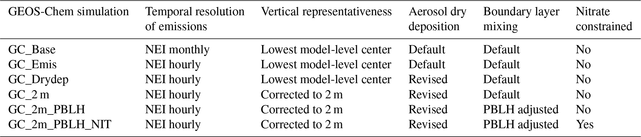
2.1 General description

We use the GEOS-Chem chemical transport model version 12.6.0 (http://www.geos-chem.org, last access: 6 October 2023) driven by the GEOS-5 Forward Processing (GEOS FP) assimilated meteorology from the NASA Global Modeling and Assimilation Office (GMAO) to examine the factors controlling the diel PM_2.5 mass variations. Prior applications of the model to PM_2.5 studies include but are not limited to evaluating and improving mechanisms affecting PM_2.5 (Zheng et al., 2015; Marais et al., 2016; Song et al., 2021; Travis et al., 2022), source attribution (Meng et al., 2019; McDuffie et al., 2021; Pai et al., 2022), assessments of the effects of horizontal transport on local air quality (Lang et al., 2013; Zhang et al., 2019; Xu et al., 2023), and exposure assessments (Kodros et al., 2016; van Donkelaar et al., 2021).

GEOS-Chem simulates detailed tropospheric aerosol–oxidant chemistry, which includes the sulfate–nitrate–ammonium system (Park et al., 2004; Fountoukis and Nenes, 2007), black carbon (Wang et al., 2014), organic carbon, secondary organic aerosol (Pai et al., 2020), mineral dust (Fairlie et al., 2007), and sea salt (Jaeglé et al., 2011). The so-called “simple” scheme (Kim et al., 2015) is used for simulating secondary organic aerosol (SOA). Absorption of radiation by brown carbon is implemented, following Hammer et al. (2016). We use nested simulations over the contiguous US in 2016 at $\mathrm{0.25}{}^{\circ }\times \mathrm{0.3125}{}^{\circ }$ over 47 vertical layers extending from the surface up to 0.1 hPa. The surface level extends from ground to about 120 m. GEOS FP is used for meteorological inputs, which includes hourly surface variables and 3-D variables at every 3 h. A global simulation at $\mathrm{2}{}^{\circ }\times \mathrm{2.5}{}^{\circ }$ is used to provide boundary conditions for the nested domain. The non-local scheme implemented by Lin and McElroy (2010) is used for boundary layer mixing.

In this work, we first evaluate the base simulation of GEOS-Chem (denoted as GC_Base in Table 1). We identify the biases of diel PM_2.5 variation in the base simulation by comparison with in situ observations. Then we develop different model components affecting PM_2.5 concentrations and conduct sensitivity simulations to explore the driving forces of diel PM_2.5 variation. Sections 2.2 and 2.3 introduce the emission configuration and default parameterization of dry deposition in GC_Base.

2.2 Emissions configurations in GC_Base

To investigate the impacts of anthropogenic emissions, we begin with the monthly version of the National Emissions Inventory (NEI) in GC_Base instead of the default hourly version in the standard nested GEOS-Chem model over North America, which is consistent with most regions outside of the contiguous US, where anthropogenic emissions at hourly resolution are often not readily available. We scale the NEI emissions from the base year of 2011 to 2016, using air pollutant emissions trend data provided by the U.S. Environmental Protection Agency (EPA; https://www.epa.gov/air-emissions-inventories/air-pollutant-emissions-trends-data, last access: 6 October 2023a). Point sources in the NEI inventory are all vertically resolved, which mainly include large industrial facilities, power plants, and airports. Nonpoint sources mainly include residential heating, transportation, commercial combustion, and solvent use. We do not use the NEI 2016 inventory, since that inventory is only available at monthly resolution in GEOS-Chem. For wildfires, we use GFED4 (Giglio et al., 2013) 3 h emissions. For dust, we use the hourly offline inventory developed by Meng et al. (2021).

2.3 Dry-deposition parameterization in GC_Base

Dry deposition of PM_2.5 in our base GEOS-Chem simulation generally follows the Zhang et al. (2001) scheme (henceforth Z01), which parameterizes particle dry-deposition velocities (V_d) by accounting for gravitational settling (V_g), aerodynamic resistance (R_a), and surface resistance (R_s), as shown in Eq. (1):

$$\begin{array}{}\text{(1)}& V_{\mathrm{d}}=V_{\mathrm{g}}+{\displaystyle \frac{\mathrm{1}}{R_{\mathrm{a}}+R_{\mathrm{s}}}}.\end{array}$$

Gravitational settling represents the particle settling due to gravity. Aerodynamic resistance describes the turbulent transport of scalars within the surface layer. Surface resistance, as formulated in Eq. (2), quantifies particle-surface contact in close proximity to surfaces by Brownian diffusion (E_b), impaction (E_Im), and interception (E_In).

$$\begin{array}{}\text{(2)}& R_{\mathrm{s}}={\displaystyle \frac{\mathrm{1}}{{\mathit{\epsilon }}_{\mathrm{0}}{u}_{\ast }(E_{\mathrm{b}}+E_{\text{Im}}+E_{\text{In}})R_{\mathrm{1}}}},\end{array}$$

where u_∗ denotes friction velocity, R₁ denotes a bounce correction term, and ε₀ denotes an empirical coefficient. Brownian diffusion contributes to dry deposition through diffusion when particles are close to surface collectors. Impaction describes the direct collision of particles to the surface due to inertia when particles move along the streamlines around collector surfaces. Interception represents the deposition by which particles are captured by surface collectors when their distances to the collectors are shorter than the radius of a single particle.

The standard GEOS-Chem dry-deposition module used in our base simulation calculates dry-deposition velocity ($V_{\mathrm{d}}^{\prime }$), following Eq. (3), where gravitational settling is ignored.

$$\begin{array}{}\text{(3)}& V_{\mathrm{d}}^{\prime }={\displaystyle \frac{\mathrm{1}}{R_{\mathrm{a}}+R_{\mathrm{s}}}}\end{array}$$

The dry deposition of PM_2.5 includes sulfate, nitrate, ammonium, organics, black carbon, fine-mode sea salt, and fine-mode mineral dust components. Information about particle size is important, as all terms in Eqs. (1)–(3) are size dependent, except aerodynamic resistance R_a. The dry-deposition module in the base GEOS-Chem simulation has inconsistencies with other GEOS-Chem modules that we address in Sect. 5.2. In the standard GEOS-Chem dry-deposition module, fine-mode mineral dust is considered in two size bins, with mass-weighted mean diameters of 1.46 and 2.80 µm. Other components are each considered in a single size bin, with mass-weighted mean dry diameters for sulfate, nitrate, ammonium, organics, black carbon, and fine-mode sea salt of 0.5 µm. Monodisperse size distributions are used for all size bins. The effect of hygroscopic growth on deposition is only considered for fine-mode sea salt, following Lewis and Schwartz (2006). We use the standard GEOS-Chem dry-deposition module for our base simulation.

3 In situ measurements of PM_2.5

The in situ measurements from the United States Environmental Protection Agency's Air Quality System (AQS) are used to evaluate the GEOS-Chem simulations. There were 451 sites operating in 2016 across the contiguous US which provided hourly PM_2.5 concentrations using a Federal Equivalent Method (FEM). As depicted in Fig. 1, 66.3 % of these FEM sites are equipped with the Met One BAM-1020 mass monitor using beta attenuation, 10.0 % with the Thermo Scientific 5014i/FH62C14-DHS monitor using beta attenuation, 7.4 % with the Thermo Scientific TEOM 1405-DF dichotomous monitor using a filter dynamics measurement system (FDMS) gravimetric, and 6.5 % with the Thermo Scientific 5030 SHARP monitor using beta attenuation. These four types of FEM monitors are used for hourly analysis in this work. The other five types of FEM instruments, contributing less than 10 % of all hourly measurements, are excluded to avoid risk of aliasing instrument-dependent and regionally dependent characteristics. Further detail about instrumentation is provided in Sect. S1 in the Supplement. A small fraction (0.05 %) of the FEM measurements exceeding 10 times their standard deviation are indicative of strong fire contamination and present significant modulation on the regional diel variation pattern and are thus excluded as outliers from the focus of this study. Also shown in Fig. 1 are the additional 737 sites using the Federal Reference Method (FRM) to measure 24 h average PM_2.5 concentrations, which significantly improve the observational coverage of the contiguous US for the evaluation of spatial distribution of GEOS-Chem simulated PM_2.5. To compare with GEOS-Chem, each site is matched with the GEOS-Chem grid nearest the box center. The FRM and FEM measurements used in this work are at 35 % ± 5 % relative humidity (EPA, 2007, 2021, 2023; Thermo Fisher Scientific, 2013). To match the measurement RH, the GEOS-Chem PM_2.5 and its composition were calculated considering the corresponding hygroscopic growth following standard practice in GEOS-Chem (GEOS-Chem Aerosols Working Group, 2021).

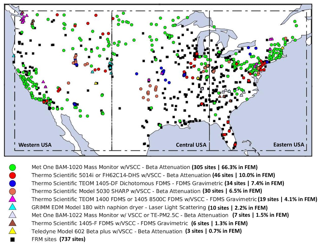
Figure 1 Spatial distribution of the U.S. EPA PM_2.5 measurements. Colored markers represent the Federal Equivalent Method (FEM) sites equipped with different kinds of instruments which report hourly PM_2.5 concentrations. Black squares represent Federal Reference Method (FRM) sites which report 24 h average PM_2.5.

4 Diel PM_2.5 variation in the base GEOS-Chem simulation and the FEM measurements

We first examine the diel PM_2.5 variation in the base simulation. Figure 2a shows the annual mean diel PM_2.5 variation across the contiguous US from the FEM in situ observations and the space and time co-located base GEOS-Chem simulation. The observed PM_2.5 exhibits a typical diel cycle consistent with previous work (Manning et al., 2018). Concentrations peak at 8:00 LT, diminish until late afternoon, increase in the evening, and remain elevated throughout the night. The base GEOS-Chem simulation broadly captures these features with their timings accurate within 1–3 h. The simulated concentration decreases from morning to late afternoon and then increases throughout the evening, consistent with the diel cycle of growth and collapse of the boundary layer. However, the simulated PM_2.5 is significantly overestimated at night, especially from midnight to early morning when the GEOS-Chem PM_2.5 increases beyond the standard deviation of the observations, during which time the observations exhibit a slight decrease. The nighttime model overestimation leads to a 106 % positive bias in the PM_2.5 diel amplitude, which is defined as the difference between the maximum and the minimum of the normalized diel concentration. The root mean square deviation (RMSD) of the annual diel variation in PM_2.5 between the base simulation and the observations is 2.18 µg m⁻³. The spatial distribution of PM_2.5 in the base GEOS-Chem simulation is discussed in Sect. S2.

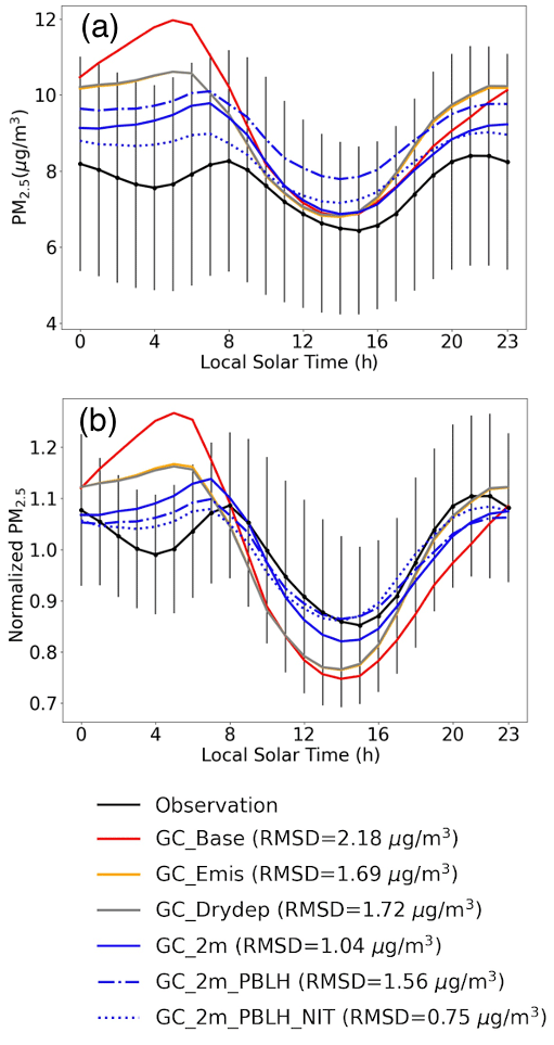
Figure 2 (a) Annual mean diel PM_2.5 variation over the contiguous US in 2016. (b) Normalized annual mean diel PM_2.5 from GEOS-Chem (GC) sensitivity simulations over the contiguous US in 2016. Vertical lines indicate the spatial standard deviations of annual mean PM_2.5 for the FEM measurements at each hour.

We classify each FEM measurement and the corresponding GEOS-Chem simulation into urban and rural using the Global Rural–Urban Mapping Project (GRUMP) v1 (Balk et al., 2006) data at 30 s resolution. Results (Fig. S3) indicate that the observed diel variations in the PM_2.5 in urban and rural areas across the contiguous US are highly consistent (r=0.97). Both urban and rural sites exhibit the same bimodal patterns, with PM_2.5 peaks near 08:00 and 21:00 LT and minima near 04:00 and 16:00 LT. The PM_2.5 dips near 04:00 and 16:00 LT are deeper over urban regions than over rural regions, which may reflect stronger vertical mixing from the urban heat island effect (Travis et al., 2022). The consistency of diel PM_2.5 variation across urban and rural locations implies a dominant role from natural processes.

Figure 3a shows the annual mean diel variation in the PM_2.5 chemical composition in the base GEOS-Chem simulation for the contiguous US. Sulfate was the least variant component throughout the day. All other components exhibit notably higher concentration at night than during the day. The pronounced PM_2.5 accumulation overnight in the base case simulation is driven primarily by nitrate, of which the mass concentrations increase by 34.1 % overnight (00:00–06:00 LT). This is consistent with the reported overestimation of nighttime nitrate in GEOS-Chem by recent studies (Miao et al., 2020; Zhai et al., 2021; Travis et al., 2022). Concentrations of ammonium and SOA, which increased by 22.2 % and 14.2 % overnight (00:00–06:00 LT), contributed to the overnight PM_2.5 accumulation to a lesser extent. Except for dust, concentrations of all other components increase from midnight to early morning, indicating that there are uniform drivers on PM_2.5 diel variation across composition.

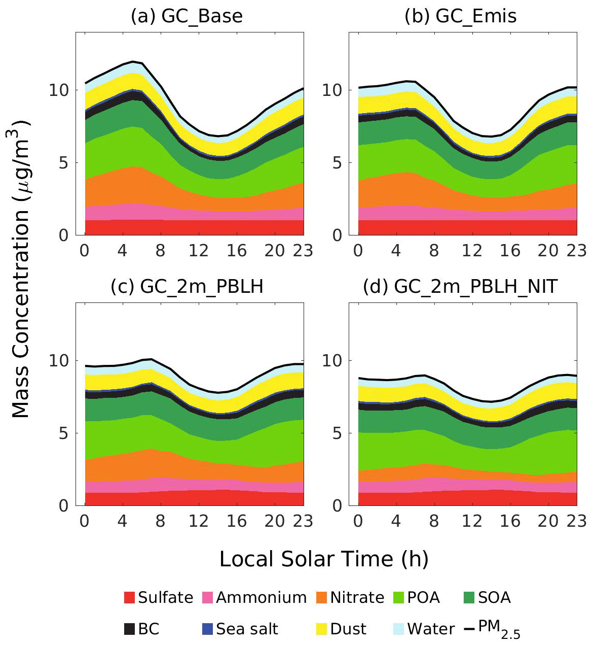
Figure 3 Annual diel profiles of PM_2.5 composition over the contiguous US in the GEOS-Chem simulations (Table 1). POA, SOA, and BC refer to primary organic aerosol, secondary organic aerosol, and black carbon, respectively. All components represent dry mass. The aerosol water associated with sulfate, nitrate, ammonium, POA, SOA, and sea salt is grouped into the water category.

5 Development of processes affecting simulation of diel PM_2.5

We develop and evaluate the processes affecting the simulation of diel PM_2.5 variation in GEOS-Chem with particular attention to the driving forces of the nighttime bias. We focus on the temporal resolution of emissions, aerosol dry deposition, vertical representativeness, boundary layer mixing, dew formation, and nitrate, as summarized in Table 1.

5.1 Impacts from the temporal resolution of emissions

We initially examine the temporal resolution of anthropogenic emissions as a source of the nighttime PM_2.5 positive bias identified in Sect. 4. Figure 4 shows the normalized mean diel emission profile for different species in the hourly version of the NEI inventory. Anthropogenic emissions are notably higher during the day than at night, with minima from midnight to early morning in the emission intensities for every primary species. The diel amplitude of SO₂ emissions is weakest, driven by persistent power plant emissions. NH₃ emissions have the strongest diel amplitude, driven by a temperature dependence for this predominantly agriculturally emitted species over the contiguous US (Zhang et al., 2018). Figure S4 depicts the normalized mean emission strengths for species in Fig. 4 both seasonally and regionally. The early afternoon NH₃ peak is most prominent over the central USA in summertime, in accordance with the temperature-dependent agricultural emissions of NH₃. Primary emissions of particulate organic carbon (OC) have a peak near 8:00 LT (local time), corresponding to more intense residential heating. The OC emissions in evening are strongest during winter, reflecting the seasonality of residential combustion activities (Li and Martin, 2018).

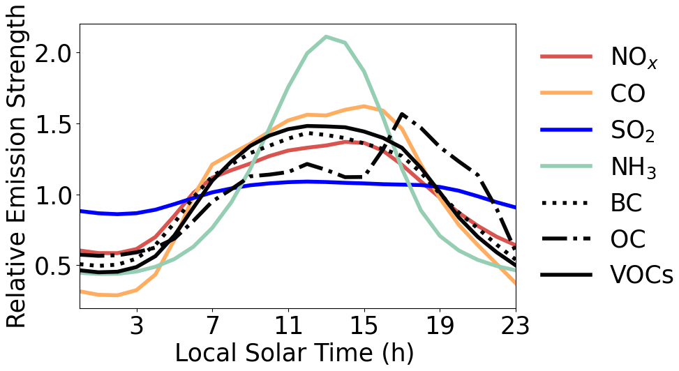
Figure 4 Normalized mean diel emission profile for different species across the contiguous US.

To evaluate the impacts from temporal resolution of emissions, we conduct a sensitivity simulation GC_Emis (Table 1) which replaces the monthly NEI in GC_Base with the hourly NEI. Figure 2b shows that GC_Emis simulates a much weaker PM_2.5 accumulation from midnight to early morning relative to GC_Base, mainly due to the lower emission intensities of aerosol sources throughout the night in the NEI hourly inventory. In the evening, PM_2.5 in the GC_Emis simulation accumulates slightly faster than in the base case, reflecting the stronger emissions in daytime after applying the hourly inventory. The RMSD between GC_Emis diel PM_2.5 and the FEM observations decreases from 2.18 µg m⁻³ in GC_Base to 1.69 µg m⁻³, and the positive bias in the diel amplitude drops from 106 % to 59 %. In terms of composition (Fig. 3b), the average mass concentrations of BC and POA overnight (00:00–06:00 LT) decrease by 25.7 % and 12.9 %, contributing the most to the reduced overnight PM_2.5 accumulation. Sulfate concentrations overnight decrease by only 3.5 %, due to weak day–night contrast in SO₂ emissions. Nitrate and ammonium concentrations decrease by only 7.1 % and 6.3 %, reflecting the relatively minor role of primary emissions versus secondary production for these two species. In GC_Emis, nitrate still accumulates notably (by 23.1 %) from 00:00 to 06:00 LT, acting as the major contributor of the PM_2.5 nighttime bias. Overall, the temporal resolution of emissions explains 44 % of the bias in simulated diel amplitude. Daytime PM_2.5 is insensitive to changes in diel emission profiles. During the night, the impacts of emissions on PM_2.5 levels are more prominent, especially from midnight to early morning when the boundary layer is more stable. From this perspective, the slight overnight reduction in the PM_2.5 in the FEM measurements is likely driven by the sharp decline in anthropogenic emissions.

The above analysis indicates the importance of using hourly emissions to simulate diel PM_2.5 variation. However, over most regions worldwide, only monthly emissions are available, with crude diel scaling factors from specific regions as a possible proxy for hourly emissions. To assess the performance of such diel scalars in simulating diel PM_2.5, we conducted three supplementary sensitivity simulations in Table S2 in which the sector- or species-specific diel scaling factors (Fig. S5) are applied to NEI and Community Emissions Data System (CEDS) monthly emissions. Results (Fig. S6) show that the average PM_2.5 accumulation overnight (00:00–06:00 LT) among the supplementary cases is 2.6 times of that in GC_Emis, leading to stronger overestimation of PM_2.5 overnight. To optimize the model performance in simulating diel PM_2.5, hourly gridded emissions are preferred over using monthly emissions with scaling factors. Nevertheless, the diel emission profile does not fully explain the diel biases identified in Sect. 4. Other contributing factors exist.

5.2 Impacts from the dry-deposition parameterizations

We explore dry deposition as the second potential source for the diel-varying biases in the base GEOS-Chem simulation. First, as described in Sect. 2.3, the dry-deposition scheme in the base GEOS-Chem model does not account for gravitational settling V_g, which leads to systematic underestimation in particle dry-deposition velocities. To improve on this missing consideration, we strictly follow Eq. (1) of Zhang et al. (2001), thus updating the gravitational settling term V_g to be explicitly considered when deriving the deposition velocity (Eq. 1). Second, the parameterization of surface resistances (Eq. 2) in the base scheme was developed when few particle deposition measurements were available. Following recent observational evidence, Emerson et al. (2020) identified that the Brownian diffusion E_b in Z01, as used in the standard GEOS-Chem model, is excessive, while the contribution from interception E_In is too weak. We update the surface resistances R_s in GEOS-Chem by applying observationally constrained Brownian diffusion E_b, impaction E_Im, and interception E_In terms, following observational evidence in Emerson et al. (2020). Formulations of E_b, E_Im, and E_In are updated, following Table 2.

Table 2 Formulations for particulate gravitational setting (V_g), Brownian diffusion (E_B), interception (E_IN), and impaction (E_IM) used in the calculation of deposition velocity (V_d).

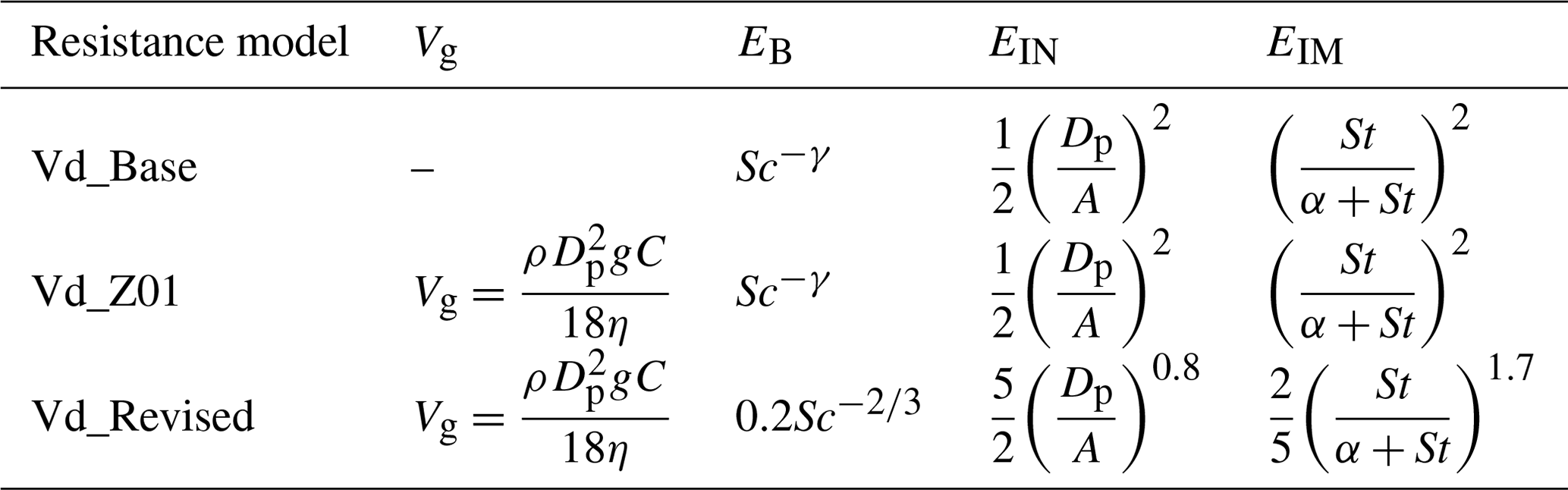
A is the characteristic radius for interception in Zhang et al. (2001). C is the Cunningham correction factor. D_p is the particle diameter. g is the gravitational acceleration constant. Sc is the Schmidt number. St is the Stokes number. V_g is the gravitational settling velocity. α is the LUC-specific constant used in the impaction efficiency in Zhang et al. (2001), where LUC represents land use classification. γ is the LUC-specific exponent used in the Brownian diffusion efficiency in Zhang et al. (2001), which ranges from 0.5 to 0.58. ρ is the density of the particle. η is the viscosity of air.

Figure 5a shows V_g as a function of particle diameter for the base (Vd_Base) and revised (Vd_Revised) parameterizations, as well as according to the Z01 scheme (Vd_Z01). A comparison of the Vd_Base and Vd_Z01 curves indicates that the inclusion of V_g in the calculation of V_d for the Vd_Z01 case substantially increases dry-deposition velocities for particles larger than 2 µm in diameter. The Vd_Revised curve indicates that implementing observational constraints on the surface resistances shifts the minimum in V_d to a particle diameter of around 0.1 µm, thus reflecting a weakened Brownian diffusion term and an enhanced interception term. Emerson et al. (2020) found that the parameterized size-dependent particle dry-deposition velocities are more consistent with observations after implementing these observational constraints. To further evaluate the impact of the particle V_d on diel PM_2.5, the representation of aerosol size distributions in the dry-deposition scheme of GEOS-Chem, including hygroscopic growth, must be considered.

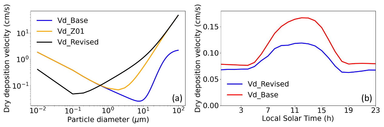
Figure 5 (a) Size-resolved particle dry-deposition velocities over the grassland land type from GEOS-Chem. (b) Diel mean dry-deposition velocities for sulfate aerosol over the contiguous US in 2016. Vd_Base represents the default dry-deposition scheme in the base GEOS-Chem model (Eq. 3). Vd_Z01 includes the effect of gravitational settling on Vd_Base (Eq. 1). Vd_Revised further implements the observational constrains on the surface resistance terms, as discussed in Sect. 5.2.

As introduced in Sect. 2.3, the dry-deposition scheme in the standard GEOS-Chem model assigns a single unreferenced mass-weighted mean diameter to different PM_2.5 components. We update the mass-weighted mean diameter for each aerosol species that was dry deposited to be consistent with the sizes in the GEOS-Chem radiation module. We implicitly consider aerosol size distributions based on mass conservation principles:

$$\begin{array}{}\text{(4)}& \begin{array}{rl}\underset{\mathrm{0}}{\overset{\mathrm{\infty }}{\int }}n\left(D_{\mathrm{p}}\right)& \cdot {\displaystyle \frac{\mathrm{4}}{\mathrm{3}}}\mathit{\pi }{\left({\displaystyle \frac{D_{\mathrm{p}}}{\mathrm{2}}}\right)}^{\mathrm{3}}\cdot \mathit{\rho }\cdot V_{\mathrm{d}}\left(D_{\mathrm{p}}\right)\mathrm{d}{D}_{\mathrm{p}}\\ & =N\cdot V_{\mathrm{d}}\left(D_{\mathrm{p}}^{\ast }\right)\cdot {\displaystyle \frac{\mathrm{4}}{\mathrm{3}}}\mathit{\pi }{\left({\displaystyle \frac{D_{\mathrm{p}}^{\ast }}{\mathrm{2}}}\right)}^{\mathrm{3}}\cdot \mathit{\rho },\end{array}\end{array}$$

where D_p denotes particle diameter, n(D_p) represents the particle number size distribution, ρ denotes the particle density, V_d(D_p) denotes the size-dependent particle dry-deposition velocity, N denotes the total particle number concentration integrated across the aerosol size distribution, $D_{\mathrm{p}}^{\ast }$ denotes the mass-weighted mean dry diameter for a specific aerosol species, and $V_{\mathrm{d}}\left(D_{\mathrm{p}}^{\ast }\right)$ denotes the dry-deposition velocity of a particle with diameter of $D_{\mathrm{p}}^{\ast }$. The size distribution for each PM_2.5 component is from Latimer and Martin (2019). The updated mass-weighted mean dry diameter is 0.17 µm for sulfate, nitrate, ammonium, and organic aerosols, is 0.23 µm for fine-mode sea salt, and is 0.67 and 2.49 µm for the fine-mode mineral dust in two size bins.

The standard GEOS-Chem dry-deposition module only considers the hygroscopic growth of fine-mode sea salt. Omitting hygroscopicity for other PM_2.5 components may lead to biases in the simulated dry-deposition velocities and thus affect the diel variation in the PM_2.5. Here we implement hygroscopic growth in the dry-deposition parameterization for sulfate, nitrate, ammonium (SIA), and organic aerosol (OA) of PM_2.5 by application of a κ-Kohler growth function to the mass-weighted mean dry diameters (Petters and Kreidenweis, 2007, 2008, 2013; Latimer and Martin, 2019). Dust and black carbon are treated as hydrophobic. The κ-Kohler growth factor is calculated as

$$\begin{array}{}\text{(5)}& \text{GF}=\left(\mathrm{1}+\mathit{\kappa }{\displaystyle \frac{\text{RH}}{\mathrm{100}-\text{RH}}}\right).\end{array}$$

The hygroscopicity parameter κ is set as 0.61 for SIA and is set as 0.1 for OA (Latimer and Martin, 2019). Efflorescence transitions are considered for the SIA components (Latimer and Martin, 2019). For fine-mode sea salt, we continue to use the growth function from Lewis and Schwartz (2006).

Taking the sulfate component in PM_2.5 as an example, Fig. 5b presents the combined impacts of all the updates above on the diel dry-deposition velocities. Implementation of the gravitational settling and hygroscopic growth tends to increase the sulfate dry-deposition velocity, compensating for the lower revised aerosol dry-deposition velocities, mainly due to the revised scheme using a smaller mass-weighted mean dry diameter. The reductions in the deposition velocity in the revised case are more prominent during daytime, when the size-dependent surface resistances dominate the dry-deposition processes. In the revised profile, from midnight to early morning (00:00–06:00 LT), the dry-deposition velocities are 10.4 % higher than those in the evening (18:00–00:00 LT), reflecting the stronger aerosol hygroscopic growth due to higher relative humidity. We evaluate the impacts on simulated diel PM_2.5 masses in GEOS-Chem as GC_Drydep simulation (Table 1), which adds all the deposition updates to GC_Emis. Figure 2b shows that the diel PM_2.5 masses simulated by GC_Drydep and GC_Emis are almost identical. The insensitivity of diel variation in the PM_2.5 to dry-deposition updates implies that the diel PM_2.5 biases identified in Sect. 4 are unlikely to be caused by the uncertainty in the GEOS-Chem dry-deposition module.

5.3 Impacts from the vertical representativeness differences between model and observations

The third possible contributor to the PM_2.5 nighttime biases that we consider is the vertical representativeness difference between the model and observations. Given the vertical extent of the lowest model level (120 m), simulated concentrations represent an average over a greater vertical extent than the typical height of FEM measurements of about 2 m. This difference in vertical representation may be especially problematic for model–measurement comparison during periods of diabatic stability, resulting in strong near-surface concentration gradients. Vertical concentration gradients within 120 m of the surface have been widely observed for aerosol species in previous field campaigns (Sievering et al., 1994; Prabhakar et al., 2017; Franchin et al., 2018). Sievering et al. (1994) measured the vertical profiles of aerosols over the Bavarian Forest National Park in Germany using filter pack sampling and reporting 2 m concentrations lower than at 51 m for nitrate (51 %), ammonium (81 %), and sulfate (81 %). In the Utah Winter Fine Particulate Study, the PM_2.5 concentrations measured by three ground sites at Logan, Cache, Salt Lake Valley, and the Utah Valley were around 70 % of those at around 50 m measured by aircraft (Franchin et al., 2018). Thus, the PM_2.5 simulated by GEOS-Chem is intrinsically different from the FEM in situ measurements because of the mismatch of vertical sampling location.

To evaluate the impact of these vertical representativeness differences, we developed the GC_2 m simulation (Table 1) in which PM_2.5 from the lowest model level of the GC_Drydep simulation is adjusted to the height of the FEM measurements (2 m above ground). The conversion process quantifies the vertical concentration gradient of secondary PM_2.5 components by using the resistance-in-series formulation for dry deposition, following previous studies (Zhang et al., 2012; Travis and Jacob, 2019). The mathematical formula is described in Eq. (6), as follows:

$$\begin{array}{}\text{(6)}& C\left(z_{\text{2M}}\right)=[\mathrm{1}-R_{\mathrm{a}}(z_{\text{2M}},z_{\text{GBC}}\left)V_{\mathrm{d}}\right(z_{\text{GBC}}\left)\right]C\left(z_{\text{GBC}}\right),\end{array}$$

where C(z_2M) and C(z_GBC) represent the concentrations at a measurement height of 2 m and the grid box center of the GEOS-Chem surface layer (around 60 m) respectively. R_a(z_2M,z_GBC) represents the aerodynamic resistances between the measurement height and the grid box center. V_d(z_GBC) represents the dry-deposition velocity. R_a(z_2M,z_GBC) is calculated using the Monin–Obukhov similarity theory, as follows:

$$\begin{array}{}\text{(7)}& R_{\mathrm{a}}(z_{\text{2M}},z_{\text{GBC}})=\underset{z_{\text{GBC}}}{\overset{z_{\text{2M}}}{\int }}{\displaystyle \frac{\mathrm{\Phi }\left(\mathit{\zeta }\right)}{k{u}^{\ast }\mathit{\zeta }}}\mathrm{d}\mathit{\zeta },\end{array}$$

where $\mathit{\zeta }=z/L$. L denotes the Monin–Obukhov length, which is determined by surface momentum fluxes and sensible heat. Φ represents a function of stability described by Businger et al. (1971). k represents the von Karman constant, and u^∗ represents the friction velocity. The method requires a boundary condition of zero concentration at ground level. Thus, it is only applied to secondary PM_2.5 components and not primary components with surface emission fluxes. The correction method described by Eqs. (6) and (7) does not account for the impacts of relative humidity (RH) and temperature (T) differences between the lowest model level and 2 m on thermodynamic partitioning of sulfate–nitrate–ammonium (SNA) aerosol. Nevertheless, by conducting simulations of the Extended AIM aerosol thermodynamics model (Wexler and Clegg, 2002), using GEOS FP relative humidity (RH), temperature (T), and GC_2 m SNA composition at 2 m and the lowest model level, we found the impacts are insignificant overall. Higher RH at 2 m leads to SNA aerosol transition from solid to aqueous form and only slightly increases the ratio (<5 %) of the partitioned aerosol phase in the SNA system, which usually occurs overnight.

Figure 2b shows the normalized annual diel PM_2.5 variation in the GC_2 m across the contiguous US. Comparison of GC_Drydep and GC_2 m indicates that the vertical correction effectively suppresses the excessive PM_2.5 levels from midnight to early morning and sustains the daytime concentration variation due to boundary layer mixing. The bias in diel amplitude of the corrected GC_2 m PM_2.5 is reduced to 26 % against the FEM observations. In terms of absolute concentrations, the average reduction from GC_Drydep to GC_2 m is 1.01 µg m⁻³ during 18:00–06:00 LT (nighttime), while that for 06:00–18:00 LT (daytime) is 0.11 µg m⁻³. This day–night contrast is consistent with a previous DISCOVER-AQ field study (Prabhakar et al., 2017), in which the vertical gradient of nitrate aerosols measured by aircraft was significantly greater in a stable surface layer than in a turbulent surface layer. At night, under a stable boundary layer, surface resistances are suppressed due to weaker particle impaction and interception. Aerodynamic resistances then become relatively stronger, with the resulting correction in Eq. (6) yielding a greater reduction in the PM_2.5 concentrations. During the day, as boundary layer mixing strengthens, surface resistances dominate over the aerodynamic resistances, and the correction in Eq. (6) is weaker. Resolving the vertical representativeness differences enables the GEOS-Chem simulation to better capture the timings of the observed overall PM_2.5 morning peak and afternoon minimum across the contiguous US. In the GC_Drydep simulation, the PM_2.5 morning peak is 3 h earlier than the FEM observations. After the vertical correction, in the GC_2 m simulation, the morning peak appears only 1 h ahead of the observations.

5.4 Impacts from boundary layer height

Planetary boundary layer height (PBLH) is investigated as the next possible source of the biases identified in Sect. 4. PBLH is closely related to boundary layer mixing, which significantly affects diel PM_2.5 (Du et al., 2020). We adjust the GEOS FP planetary boundary layer height (PBLH) which is used to drive GEOS-Chem by using the PBLH derived from the Aircraft Meteorological Data Reports (AMDAR) at 54 sites (Fig. S7) across the contiguous US (Zhang et al., 2020) as reference. The AMDAR PBLH is defined as the lowest level at which the bulk Richardson number exceeds a critical value of 0.5 (Zhang et al., 2020). The vertically resolved bulk Richardson number is calculated from vertical profiles of temperature, humidity, and wind speed in the AMDAR dataset.

Figure 6 shows the seasonal variation in PBLH. The observed PBLH from AMDAR shows similar diel variation across all seasons, which stays low from midnight to early morning, increases to a maximum in mid-afternoon, and then decreases throughout the rest of the day. In terms of absolute amplitude, the AMDAR PBLH is higher during spring and summer, mainly due to strong near-surface wind speed and intense solar radiation (Guo et al., 2016). The GEOS FP reanalysis generally captures the diel variation in the AMDAR PBLH over all seasons, although with overestimates during daytime (07:00–19:00 LT), which is consistent as previous comparison studies (Millet et al., 2015; Zhu et al., 2016). The daytime overestimation in GEOS FP PBLH is most likely due to excessive surface heating in the dataset. As reported in Millet et al. (2015), the daytime temperature at 2 m in GEOS FP was notably higher than that observed by ceilometer, and the diel pattern of the bias in GEOS FP temperature at 2 m matched that in the PBLH well. The average daytime AMDAR PBLH reaches a maximum in spring, which is slightly higher than that in summer, likely reflecting greater surface wind speed in spring than in summer according to the AMDAR observations and leading to greater turbulence and vertical mixing and higher PBLH. GEOS FP PBLH exhibits much higher values in summer than in spring. This inconsistency might be caused by a stronger overestimation of GEOS FP PBLH in summer which is introduced by excessive surface heating in the GEOS FP dataset (Millet et al., 2015).

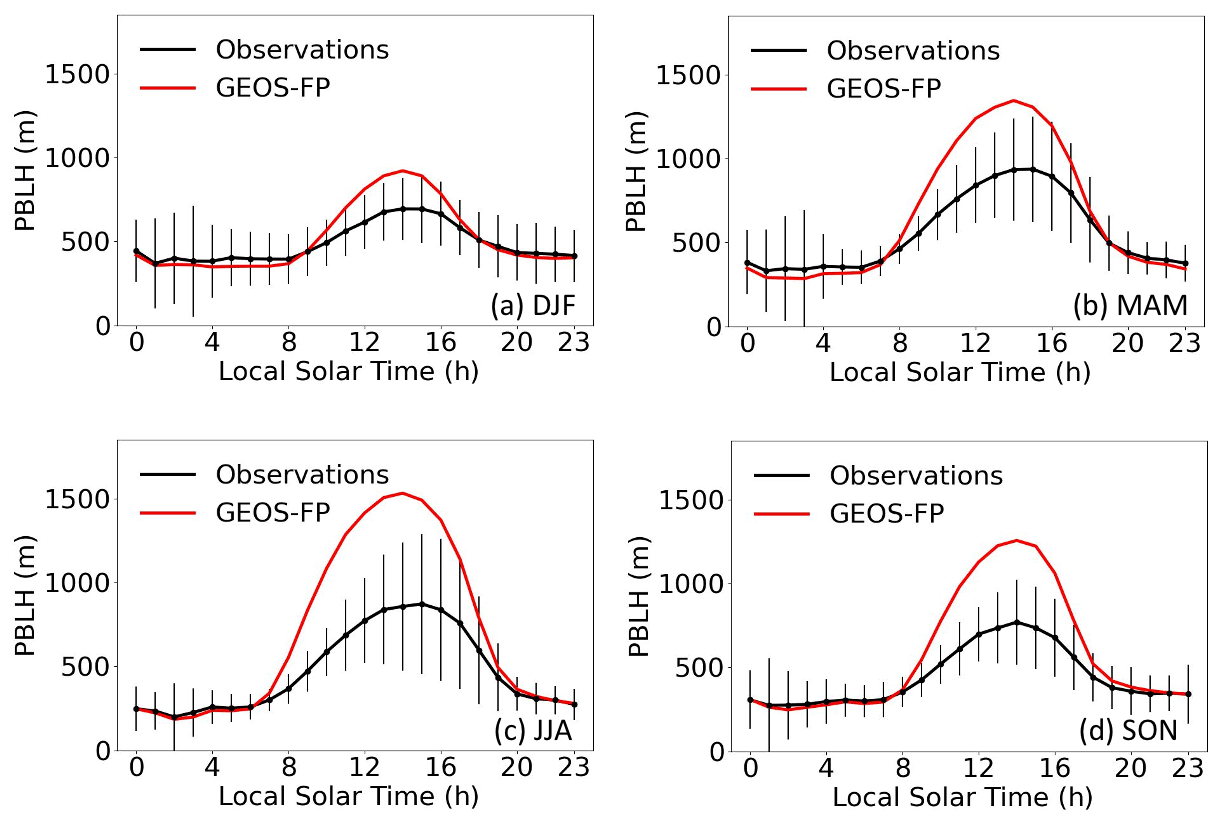
Figure 6 Seasonal diel variation in the AMDAR (observation based) and GEOS FP PBLH. Vertical bars indicate the spatial standard deviations of AMDAR PBLH.

To quantify the impacts of the uncertainty in PBLH on modeled diel PM_2.5, we develop the GC_2m_PBLH simulation (Table 1) in which the GEOS FP PBLH used in the GC_2 m simulation is adjusted by the AMDAR observations. Specifically, we matched the hourly AMDAR and GEOS FP PBLH over the contiguous US spatially and temporally and then derived USA-averaged (00:00–23:00 LT) adjustment factors for different seasons, following Eq. (8).

$$\begin{array}{}\text{(8)}& {\text{AF}}_{i,j}={\displaystyle \frac{{\stackrel{\mathrm{‾}}{{\text{PBLH}}_{\text{AMDAR}}}}_{i,j}}{{\stackrel{\mathrm{‾}}{PBL{H}_{\text{GEOS FP}}}}_{i,j}}},\end{array}$$

where AF_i,j represents the PBLH adjustment factor for season i and hour j, ${\stackrel{\mathrm{‾}}{{\text{PBLH}}_{\text{AMDAR}}}}_{i,j}$ represents the USA-averaged AMDAR PBLH for season i and hour j, and ${\stackrel{\mathrm{‾}}{{\text{PBLH}}_{\text{GEOS FP}}}}_{i,j}$ represents the USA-averaged GEOS FP PBLH for season i and hour j. Implementing this adjustment scales the GEOS FP PBLH to the same seasonal diel value as the AMDAR PBLH over the contiguous US. Applying these adjustment factors to the GEOS FP PBLH, as shown in blue and dashed lines in Fig. 2b, reduces the absolute biases in the simulated PM_2.5 diel amplitude against the FEM observations by 8 %.

5.5 Impacts from dew formation

We also examined the possibility of dew formation as a potential process affecting the diel variation in PM_2.5. It was reported that the condensation process during the formation of dew involves removal of airborne particles from the atmosphere (Polkowska et al., 2008; Muskała et al., 2015). We considered whether the observed PM_2.5 decrease from midnight to early morning (Fig. 2) might be partly ascribed to this mechanism and thus contribute to the overestimated nighttime PM_2.5. However, based on two lines of reasoning, we conclude here that dew formation is unlikely to significantly affect the diel PM_2.5 mass variations over the contiguous US. First, we examined co-located hourly RH and PM_2.5 mass concentrations at 37 sites in 2016 across the contiguous US. Figure 7 shows four examples. We found no evidence of correlation of low PM_2.5 masses and high nighttime RH values (r=0.16 for Johnson, Kansas; r=0.18 for Jackson, Missouri; r=0.13 for Summit, Ohio; r=0.15 for Jefferson, Kentucky). Second, the decreases in the PM_2.5 overnight are found sharpest in the western USA, where the average relative humidity (RH) is lowest among all subregions, which indicates that dew formation at high RH condition is unlikely an important driving factor.

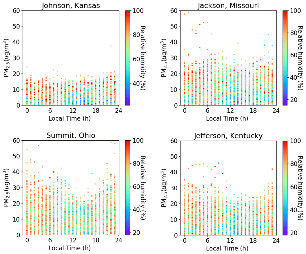
Figure 7 Co-located relative humidity (RH) and PM_2.5 mass concentrations at four example sites. Each point represents the measured hourly PM_2.5 concentration at the measured hourly RH for each site. The RH measurements are provided by the NOAA Local Climatological Data (LCD) program. The PM_2.5 mass concentrations are provided by the U.S. EPA FEM sites.

5.6 Impacts from nitrate aerosols

In Fig. 3b, hourly emissions reduce nighttime concentrations of nitrate and organics, primarily reflecting diminished nighttime emissions of NH₃, NO_x, and organic carbon. Accounting for vertical representativeness further reduces nighttime concentrations of nitrate (Fig. 3c), leading to reduced positive biases of 24 h averaged nitrate mass against in situ observations (Fig. S8). Nevertheless, positive nitrate biases remain in the GC_2m_PBLH simulation (Fig. S8), which has been a long-standing issue in GEOS-Chem (Heald et al., 2012; Zhu et al., 2013). According to recent works (Miao et al., 2020; Zhai et al., 2021; Travis et al., 2022), uncertainties in aerosol uptake coefficient for N₂O₅ and NO₂, underestimated dry deposition of HNO₃, and overly shallow nighttime mixing layer are possible contributors. But none of these fully resolve the diel biases of nitrates in GEOS-Chem, indicating that the biases are likely caused by misrepresentation in both chemistry and meteorology in the model. Following analyses by Travis et al. (2022) over Seoul, South Korea, we conducted sensitivity simulations (Sect. S3) and found that N₂O₅ hydrolysis dominates the nighttime nitrate production (Figs. S9 and S10) in our simulations over the contiguous US, which is consistent with a previous work (Alexander et al., 2020). As shown in Fig. S9, turning off N₂O₅ hydrolysis largely reduces the PM_2.5 biases from midnight to early morning and yields a diel PM_2.5 variation that is highly consistent with observations. The bias in simulated nitrate mass concentrations is also reduced by turning off N₂O₅ hydrolysis (Fig. S8). The results indicate that the N₂O₅ hydrolysis overnight might be excessive in the model. It is also possible that the performance of the simulation without N₂O₅ hydrolysis on aerosols is an indicator of multiple chemical and physical processes affecting nitrate, as explored by Miao et al. (2020), Zhai et al. (2021), and Travis et al. (2022). While the full origins of the GEOS-Chem nitrate bias remain unknown, we examine the effects of constraining nitrate concentrations on PM_2.5 by developing the GC_2m_PBLH_NIT simulation, in which the modeled nitrate concentrations are halved from GC_2m_PBLH to better represent the contiguous US average of in situ observations (Fig. S8). The bias of the diel amplitude of PM_2.5 in GC_2m_PBLH_NIT against FEM observations is reduced to −12 % (Fig. 2). The total aerosol water concentration decreases by 12.7 % in GC_2m_PBLH_NIT from GC_2m_PBLH as nitrate is reduced. These results motivate further investigation of the nitrate bias in GEOS-Chem.

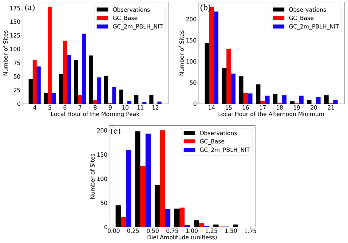
Figure 8 Distribution of simulated and observed PM_2.5 features over the FEM sites. (a) Timing of morning peak. (b) Timing of afternoon minimum. (c) Diel amplitude.

6 Discussion of diel PM_2.5 variation in the final revised GEOS-Chem simulation (GC_2m_PBLH_NIT)

Overall, updating the temporal resolution of emissions, dry-deposition parameterizations and boundary layer height and resolving the vertical representative differences between the model and observations and constraining nitrate notably improves the diel variation in the PM_2.5 in GC_2m_PBLH_NIT relative to GC_Base for both urban and rural regions (Fig. S3) in a similar way. In the annual diel comparison averaged across the contiguous US (Fig. 2), the bias in the PM_2.5 diel amplitude in GC_2m_PBLH_NIT (−12 %) is significantly reduced relative to GC_Base (106 %). The average observed PM_2.5 morning peak and afternoon minimum are at 08:00 and 15:00 LT, respectively. GC_Base simulates them with biases of −3 and −1 h, while GC_2m_PBLH_NIT agrees with observed timing within 1 h. In addition to the average comparison across the country, we further explore the performances over all FEM sites. Figure 8 shows histograms of the timing of the morning peak, of the afternoon minimum, and of the diel amplitude. At most FEM sites, GC_Base tends to overestimate the PM_2.5 diel amplitude and simulates the PM_2.5 diel features too early. By correcting for the vertical representativeness differences, using emissions with hourly temporal resolution, adjusting the GEOS FP boundary layer heights, and constraining nitrate concentrations, these biases are largely addressed in GC_2m_PBLH_NIT with the distribution in the histogram and thus match the observations better. The RMSD of diel PM_2.5 between GC_2m_PBLH_NIT and the FEM observations decreases from 2.18 to 0.75 µg m⁻³. With the reduced 24 h averaged PM_2.5 concentration, GC_2m_PBLH_NIT also improves the agreements of annual mean PM_2.5 against the FEM/FRM measurements across the contiguous US (Sect. S2).

Figure 9 shows the diel variation in the PM_2.5 in different seasons and subregions. The observed diel PM_2.5 variations are generally similar to the annual results across the country, suggesting consistent mechanisms controlling the local cycles. The observed PM_2.5 diel amplitude is smallest during summer, as the observed concentrations decrease more slowly from mid-morning to late afternoon than in other seasons. The GC_2m_PBLH_NIT simulation generally reproduces this summer minimum in the diel amplitude, thus improving on GC_Base, which simulates the minimum amplitude in winter, by reducing excess PM_2.5 at night, by reducing PM_2.5 precursor emissions, by accounting for vertical representativeness differences at night, by adjusting boundary layer height using aircraft observations, and by constraining nitrate. Stronger photochemical production of PM_2.5 occurs more during the daytime in summer than other seasons, which also counteracts the ventilation by boundary layer mixing. The RMSD between GC_2m_PBLH_NIT and observed diel PM_2.5 improves on GC_Base for most seasons and subregions (Table S1 in the Supplement).

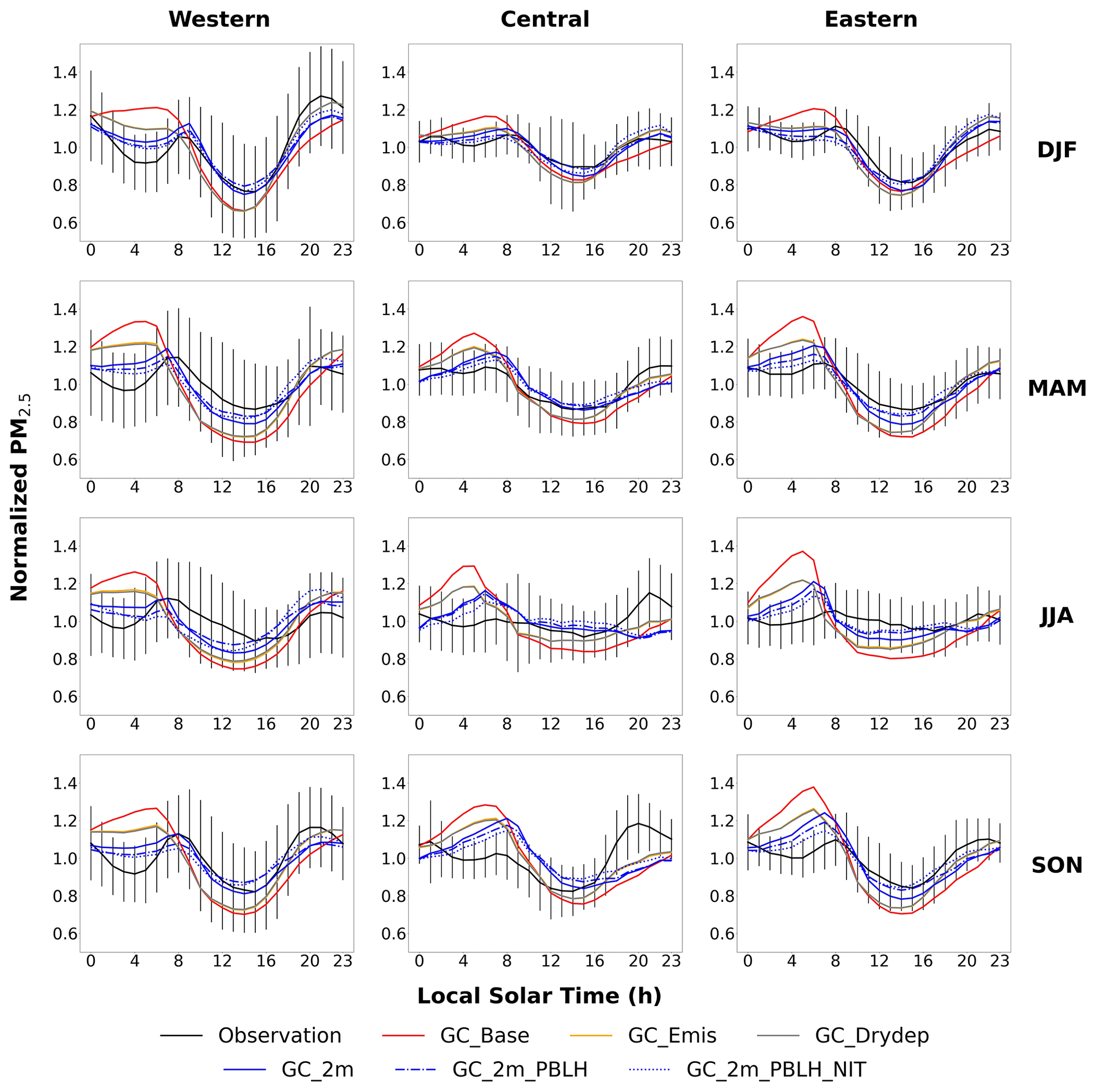
Figure 9 Seasonal and regional diel profiles of GEOS-Chem PM_2.5 from different simulation designs (Table 1). Vertical lines indicate the spatial standard deviations of seasonal mean PM_2.5 for the FEM measurements at each hour in a certain subregion.

Overall, we find that the driving forces of the typical diel PM_2.5 mass variation over the contiguous US reflects a complex interplay of planetary boundary layer dynamics, emissions, and photochemistry. The initial concentration peak in the mid-morning occurs as combustion activities are emitted into a shallow mixed layer. Subsequent ventilation by vertical mixing dominates as the boundary layer develops, leading to a decrease in PM_2.5 until late afternoon, despite the enhanced photochemical production. The subsequent collapse at the mixed layer during sunset confines PM_2.5 emissions to the surface layer, with a relative higher but diminishing concentration throughout the night as low nocturnal emissions foster a concentration minimum or flatness between midnight and early morning (Fig. 9). To further reveal the underlying driving forces, we focus on several example sites on which GC_2m_PBLH_NIT reproduces the observed overnight PM_2.5 variation well. Figure 10 shows four example sites, where the PM_2.5 concentrations overnight in the GC_Base simulation are substantially overestimated. By accounting for the hourly variation in anthropogenic emissions, in GC_Emis, the simulation starts to successfully reproduce the PM_2.5 decrease or flatness overnight. By further correcting for the vertical representativeness differences, adjusting the boundary layer height, and constraining nitrate, in GC_2 m, GC_2m_PBLH, and GC_2m_PBLH_NIT, the simulations more closely represents the FEM measurements. These sensitivity simulations reinforce the notion that the internal driving forces of the PM_2.5 minimum or flatness from midnight to early morning reflect a combination of the decrease in the anthropogenic emissions by weaker anthropogenic activities, while resolving the vertical representativeness differences between model and observations.

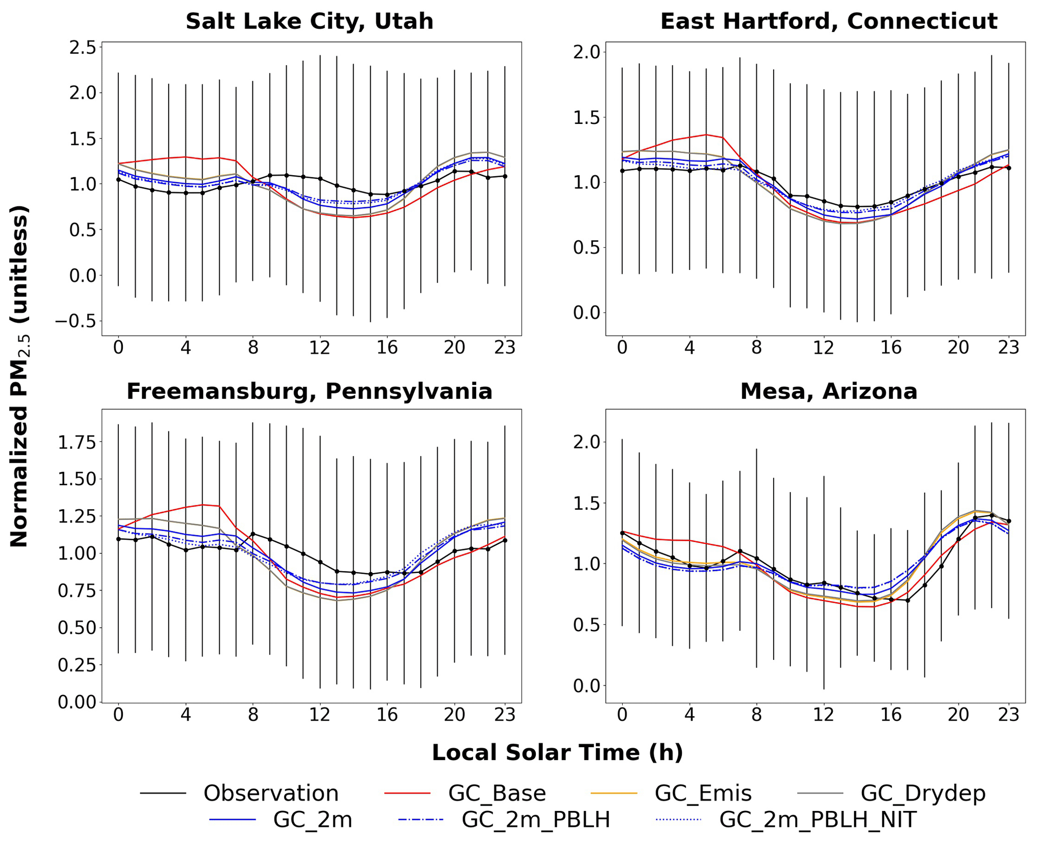
Figure 10 Diel PM_2.5 mass variation in the GEOS-Chem simulations (Table 1) and the in situ measurements over four example FEM sites.

Despite the pronounced improvement in simulating the PM_2.5 diel variation, positive biases remain in early morning in most regions and seasons (Fig. 9). The regional and seasonal variation in PM_2.5 chemical composition offers insight (Fig. S11). Nitrate appears to be an important contributor to the bias, which is not fully understood, as discussed in Sect. 5.6. Insufficient vertical and horizontal resolution in our simulations to fully resolve the nocturnal stratification and horizontal source separation (Zakoura and Pandis, 2018; Boys, 2022) are possible contributors. The remaining evening bias in the spring, summer, and winter in central USA could reflect the possible underestimation of residential emissions in NEI (Trojanowski et al., 2022). Figure S4 shows that the OC emissions as relevant indicators of residential combustion are the weakest in the evenings for spring, summer, and winter in central USA.

In summary, emissions, vertical representativeness differences between model and observations, boundary layer mixing, and nitrate are found to be the top four contributing factors of the diel biases in GEOS-Chem PM_2.5. Dry deposition and scavenging by the formation of dew are relatively unimportant. The vertical correction for the representativeness differences by using the resistance-in-series method is critical for improving the simulation of the PM_2.5 diel amplitude and capturing the timings of the observed PM_2.5 morning peak and afternoon minimum, thus indicating the significance of vertical resolution of GEOS-Chem for simulating the diel PM_2.5 variation. Reducing the daytime positive biases in GEOS FP PBLH and improvements in the diel representation of residential combustion may be useful to further improve the diel PM_2.5 in GEOS-Chem. In addition to the above impacting factors, we emphasize the necessity of conducting simulations at a fine spatial resolution to resolve processes affecting diel variation in PM_2.5 concentrations. Comparison of the GEOS-Chem simulations at $\mathrm{0.25}{}^{\circ }\times \mathrm{0.3125}{}^{\circ }$ and $\mathrm{2}{}^{\circ }\times \mathrm{2.5}{}^{\circ }$ against the FEM observations (Fig. S12) reveals that a higher spatial resolution better enables the model to reproduce the observed diel PM_2.5 variation through reducing the excessive PM_2.5 accumulation during nighttime (18:00–06:00 LT). At the coarse spatial resolution, the simulated PM_2.5 mass concentrations increase by 36.3 % from 18:00 to 06:00 LT, which is greater than the observed 5.8 % increase. At the finer spatial resolution, that nighttime increase in the PM_2.5 mass concentrations reduces to 20.3 %. The recent advances to the GEOS-Chem High-Performance (GCHP) model with stretched grid capabilities (Bindle et al., 2021; Martin et al., 2022) enables a higher spatial resolution than $\mathrm{0.25}{}^{\circ }\times \mathrm{0.3125}{}^{\circ }$, which could offer improved representation of resolution-dependent processes in future analyses.

7 Conclusions

In this work, we used the GEOS-Chem model in its nested configuration to interpret the observed diel variation in PM_2.5 concentration for the contiguous United States. We identified and addressed several biases of the base GEOS-Chem simulation of the diel variation in the PM_2.5 mass concentrations. (1) The simulated PM_2.5 accumulation overnight was excessive in the base simulation, which disagreed with the observed concentration decrease or flatness from midnight to early morning, leading to a significantly overestimated PM_2.5 diel amplitude in the model. (2) The simulated timings of the PM_2.5 morning peak and afternoon minima were notably earlier relative to the in situ observations, especially for the morning peak (3 h earlier).

To reveal the contributing factors to the diel PM_2.5 biases in the base simulation, we conduct sensitivity simulations in which we (1) increased the temporal resolution of anthropogenic emissions from monthly to hourly, (2) updated the dry-deposition scheme, (3) resolved the vertical representativeness differences between the model and the observations, (4) corrected for the diel biases in the boundary layer heights of the model, (5) explored the impacts from dew formation, and (6) examined the role of aerosol nitrate.

We found that several developments aided the representation of the PM_2.5 diel variation in the GEOS-Chem model. Hourly representation of emissions decreased normalized PM_2.5 concentrations at night, with increases during the day. Accounting for vertical representativeness differences between the GEOS-Chem surface layer of 120 m and the measurement height of 2 m further decreases PM_2.5 at night, leading to better representation of the timing of the morning peak (∼ 07:00 LT) and afternoon minimum. Developments to the dry-deposition scheme aided a mechanistic representation of the gravitational settling and its hygroscopic dependence, although with negligible effects on the PM_2.5 diel variation. A reduction in the simulated PBLH to represent aircraft observations also aids agreement with observed PM_2.5 diel variation. These improvements also partially addressed a long-standing issue of a positive bias in simulated nitrate concentrations, but additional constraints from nitrate observations were necessary to represent diel PM_2.5 variation. The slight PM_2.5 decrease/flatness overnight is more likely caused by diminished emissions, rather than enhanced dry deposition (Zhao et al., 2009) or dew events (Sect. 5.5). Hourly anthropogenic emissions are important for GEOS-Chem to accurately simulate diel PM_2.5 variation. Using monthly emissions combined with sector- or species-specific diel scaling factors instead can lead to higher PM_2.5 positive biases overnight. Resolving the vertical representativeness differences introduced by the subgrid vertical gradient of PM_2.5 in the surface model level contributed to capturing timings of PM_2.5 diel variation. Overall, the mean diel variation in PM_2.5 for the contiguous US is attributed to (1) growth in PM_2.5 concentrations by 10 % from early morning (04:00 LT) to mid-morning (08:00 LT), which is driven by increasing emissions into a shallow mixed layer; (2) a subsequent decline in PM_2.5 concentrations by 22 % from mid-morning (08:00 LT) to late afternoon (15:00 LT) during growth of the mixed layer; (3) a rapid increase in PM_2.5 by 30 % from late afternoon (15:00 LT) to evening (22:00 LT) as emissions persist into a collapsing mixed layer; and (4) a subsequent weak decline in PM_2.5 concentrations by 10 % as emissions diminish overnight (22:00–04:00 LT). Despite the advances in representing and understanding PM_2.5 diel variation, minor biases remain. A more mechanistic representation of nitrate is needed. The importance of the vertical resolution in representing PM_2.5 diel variation identifies an advantage to be offered by a forthcoming GEOS-6 dataset, with a planned doubled number of vertical levels in the planetary boundary layer compared to GEOS FP (NASA, 2012). Recent advances in the horizontal resolution of GEOS-Chem (Bindle et al., 2021; Martin et al., 2022) should also enable simulations with a finer spatial resolution to further improve the diel performances.