the Creative Commons Attribution 4.0 License.
the Creative Commons Attribution 4.0 License.
 | 23 Jan 2023
Climate-driven deterioration of future ozone pollution in Asia predicted by machine learning with multi-source data
Huimin Li
Jianbing Jin
Hailong Wang
Pinya Wang
Hong Liao
Ozone (O3) is a secondary pollutant in the atmosphere formed by photochemical reactions that endangers human health and ecosystems. O3 has aggravated in Asia in recent decades and will vary in the future. In this study, to quantify the impacts of future climate change on O3 pollution, near-surface O3 concentrations over Asia in 2020–2100 are projected using a machine learning (ML) method along with multi-source data. The ML model is trained with combined O3 data from a global atmospheric chemical transport model and real-time observations. The ML model is then used to estimate future O3 with meteorological fields from multi-model simulations under various climate scenarios. The near-surface O3 concentrations are projected to increase by 5 %–20 % over South China, Southeast Asia, and South India and less than 10 % over North China and the Gangetic Plains under the high-forcing scenarios in the last decade of 21st century, compared to the first decade of 2020–2100. The O3 increases are primarily owing to the favorable meteorological conditions for O3 photochemical formation in most Asian regions. We also find that the summertime O3 pollution over eastern China will expand from North China to South China and extend into the cold season in a warmer future. Our results demonstrate the important role of a climate change penalty on Asian O3 in the future, which provides implications for environmental and climate strategies of adaptation and mitigation.
- Article
(6611 KB) - Full-text XML
-
Supplement
(2335 KB) - BibTeX
- EndNote


Tropospheric ozone (O3) is a secondary air pollutant, formed by photochemical oxidation of non-methane volatile organic compounds (NMVOCs) and carbon monoxide (CO) in the presence of nitrogen oxides (NOx= NO + NO2) and sunlight. It has adverse effects on human health (Malley et al., 2017; Cakmak et al., 2018), vegetation growth (Yue et al., 2017; Mills et al., 2018), and climate change (Checa-Garcia et al., 2018; Gaudel et al., 2018). A better understanding of the causes of changes in O3 concentrations is useful for developing effective environment and climate strategies. Since the mid-1990s, Asian regions, including South Asia, East Asia, and Southeast Asia, have experienced the fastest O3 increase rate of 2–8 ppb per decade at remote surface sites and in the lower free troposphere across the world (IPCC, 2021). A number of air quality monitoring stations have been established in China since 2013 to measure real-time near-surface particulate matter, O3, and other air pollutants. The measurements showed an increasing trend of urban warm-season daily maximum 8 h average (MDA8) O3 concentrations of 2.4 ppb (5 %) yr−1 that is faster than any other regions worldwide during 2013–2019 (Lu et al., 2020). However, many regions in Asia lack O3 observations with sufficient spatial and temporal coverage. Also, most of the present regional observations are collected only near population clusters, which are not representative of the entire region (Zhou et al., 2022).
To supplement the limited near-surface O3 measurements, many studies utilized global and regional models with comprehensive physical and chemical processes to simulate O3 concentrations (Zhu et al., 2017; Gao et al., 2020; Yang et al., 2022). Moreover, statistical models have also been used to estimate O3 concentrations (Chen et al., 2020; Zhang et al., 2020). In recent years, machine learning (ML) approaches, such as random forest (Xue et al., 2020; Wei et al., 2022), neural network (Di et al., 2017), support vector machine (Su et al., 2020), extreme gradient boosting (Liu et al., 2020), and ensemble learning (Liu et al., 2022), have been widely applied to estimate O3 levels based on potential influential factors (e.g., precursor emissions, meteorological conditions, land use, surface elevation, gross domestic product, population density, and geographical variables). The abovementioned previous studies utilizing the ML methods showed high computational efficiency and accuracy, with an overall R2 between the observed and predicted O3 concentrations in the range of 0.7–0.9.
Meteorological factors and synoptic conditions play important roles in affecting O3 pollution (Fu and Tai, 2015; Gong and Liao, 2019; Yin et al., 2019; Liu and Wang, 2020; Dang et al., 2021). Gong and Liao (2019) illustrated that hot, dry, and stagnant weather conditions are favorable for the formation and persistence of severe O3 pollution over northern China. High air temperature along with intense incoming shortwave radiation accelerates both photochemical reaction rates and natural precursor emissions for O3 production (Jacob and Winner, 2009). Under high relative humidity conditions, O3 concentrations decrease due to many complex physical and chemical mechanisms (Jeong and Park, 2013; Kavassalis and Murphy, 2017; Lu et al., 2019; Li et al., 2021a). Cloud and precipitation impact O3 levels through reducing the downwelling solar radiation and washout of pollutants (Toh et al., 2013). Anomalous sea level pressure patterns can affect the long-range transport of O3 by influencing atmospheric circulation (Santurtún et al., 2015). By changing the air stagnation condition and transport of pollutants, wind fields can also affect O3 concentrations in local and downwind areas of emission sources (Doherty et al., 2013).
Future climate change corresponding to the different climate scenarios can impact O3 through altering meteorological conditions (Wang et al., 2013; Fu and Tian et al., 2019). Using regional climate fields downscaled from general circulation models to investigate potential O3 variations in the US due to changing climate, Fann et al. (2015) projected the MDA8 O3 to increase by 1–5 ppb as daily maximum average temperature increases by 1–4 ∘C in 2030 relative to 2000. Colette et al. (2015) estimated that the climate penalty for future summertime near-surface O3 reaches 0.99–1.5 ppb by the end of the 21st century (2071–2100) in Europe compared to present-day levels using an ensemble of eight global coupled climate–chemistry models under the RCP8.5 (Representative Concentration Pathway) scenario. Through fixing sea surface temperature at present-day and future conditions in five atmospheric-only models as part of AerChemMIP (Aerosol Chemistry Model Intercomparison Project), Zanis et al. (2022) projected the climate change penalties and benefits on global near-surface O3 concentrations from 2015 to 2100 under scenarios of SSP3-7.0 (Shared Socioeconomic Pathway). They found O3 reductions in most regions of the globe, except a robust O3 climate penalty of 1–2 ppb ∘C−1 in South Asia and East Asia under global warming following the SSP3-7.0 pathway. However, SSP3-7.0 is not a good representative scenario for both air quality and climate in Asia. The emissions of greenhouse gases (GHGs) and air pollutants over East Asia in SSP3-7.0 are assumed to significantly increase in the near future and remain at high levels in the middle of the 21st century, compared to SSPs (Li et al., 2022), while the emissions of air pollutants have been cut by a lot since the 2010s in the real world (Wang et al., 2021). The GHGs and pollutant emissions are very likely to continually decline in the future, related to the carbon neutrality commitment (Cheng et al., 2021).
In this study, we aim to better characterize the impact from future climate change on Asian O3 pollution using multiple state-of-the-art modeling tools and data. It is important for policymakers that mitigating global climate change potentially has positive benefits to surface air quality through meteorological factors, not only the reduction in fossil fuel co-emissions. The near-surface O3 concentrations covering 2020–2100 in Asia are projected using an ML method integrated with multi-source data, including assimilated O3 data that combine ground observations across China and simulations from a global 3-D chemical transport model (GEOS-Chem), meteorological fields under various climate scenarios from the latest Coupled Model Intercomparison Project Phase 6 (CMIP6) multi-model simulations, and other auxiliary data (e.g., emissions, land use, topography, population density, and spatiotemporal information). ML approach gives the capacity to explore many scenarios more rapidly and for longer time periods than the chemical transport model process-based modeling. Details of the data and methodology used in this study are described in Sect. 2. Section 3 analyzes the results of climate-driven O3 variations over different key regions of Asia. Section 4 summarizes the main conclusions and discusses potential uncertainties in this study.

Figure 1The structure and specific schematics for predicting future O3 concentrations under four scenarios based on the machine learning (ML) method. MET: meteorology; EMIS: emissions; LAT: latitude; LONG: longitude; MOY: month of the year (see other definitions in Table 1).
2.1 GEOS-Chem model description
Figure 1 illustrates the procedures for predicting future near-surface O3 over Asia under four scenarios. To assimilate O3 data for the ML model training, the near-surface O3 concentrations over Asia from 2014 to 2019 are firstly simulated using the nested-grid version of the 3-D GEOS-Chem model (version 12.9.3), driven by the Modern-Era Retrospective analysis for Research and Applications, Version 2 (MERRA-2), reanalysis meteorological data (Gelaro et al., 2017). The nested GEOS-Chem has 47 vertical layers from the surface up to 0.01 hPa, with a horizontal resolution of 0.5∘ latitude × 0.625∘ longitude over the Asia domain (11∘ S–55∘ N, 60–150∘ E). The lateral boundaries of chemical tracer concentrations are provided by global simulations at 2∘ latitude × 2.5∘ longitude horizontal resolution. The model includes fully coupled aerosol–O3–NOx–hydrocarbon chemical mechanisms (Park et al., 2004; Pye et al., 2009; Mao et al., 2013), with about 300 species participating in over 400 kinetic and photochemical reactions (Bey et al., 2001). The stratospheric O3 chemistry is simulated through a linearized O3 parameterization scheme (LINOZ; Mclinden et al., 2000), and the planetary boundary layer mixing is calculated by a non-local scheme (Lin and McElroy, 2010). GEOS-Chem has shown a good performance in reproducing spatiotemporal distributions of O3 concentrations (e.g., Ni et al., 2018; Li et al., 2019).
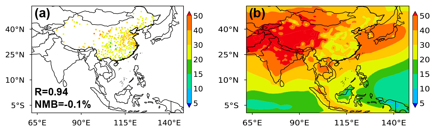
Figure 2Spatial distributions of (a) observed near-surface O3 concentrations across China and (b) assimilated O3 concentrations over Asia in 2014–2019. Correlation coefficient (R) between observed and assimilated O3 and the normalized mean bias (NMB (Observed − Assimilated) / ∑ Assimilated ×100 %) are given at the bottom left of panel (a).
The historical (2014–2019) anthropogenic emissions of O3 precursor gases, including NOx, NMVOCs, and CO, utilized in the nested domain are obtained from the Community Emissions Data System (CEDS; Hoesly et al., 2018) version 2021_04_21, which fully considered the recent emission reductions in China related to clean air measures. The biomass burning emissions are acquired from the Global Fire Emissions Database, Version 4 (GFED4; van der Werf et al., 2017). Biogenic emissions of NMVOCs from the Model of Emissions of Gases and Aerosols from Nature (MEGAN) version 2.1 are employed, with updates from Guenther et al. (2012). Soil NOx sources are calculated with an updated version of the Berkeley–Dalhousie Soil NOx Parameterization scheme (Hudman et al., 2012). NOx emissions from lightning are as described by Murray et al. (2012), and the vertical distribution of emissions follows Ott et al. (2010).
2.2 Ground O3 observations
To improve the performance of the ML model in predicting O3 concentrations, the nationwide hourly near-surface O3 concentrations in China during 2014–2019 are obtained from the Chinese Ministry of Ecology and Environment (MEE) and used for O3 data assimilation, which has been widely used to examine pollution over China in previous studies (K. Li et al., 2020, 2021; Qian et al., 2022). The observational network had about 500 monitoring sites in 2013 and expanded to more than 1500 sites after 2019, covering 360 cities in mainland China. In this study, the quality controlled hourly O3 observations in 360 cities are averaged within each 0.5∘ latitude × 0.625∘ longitude grid of the GEOS-Chem model.
2.3 Data assimilation
The assimilation system, which is used to combine the O3 observations across China with results from GEOS-Chem simulations, is based on a three-dimensional variational (3DVar) data assimilation (Kalnay, 2003; Evensen et al., 2022). The goal of the 3DVar is to find the maximum likelihood estimation of a state vector x, which represents the O3 concentrations here in this study, given the available observations y through minimizing the cost function:
where xb represents the priori simulation; B is the empirical background covariance matrix formulated as a product of the uncertainty in the simulated value and a distance-based correlation matrix C; and the individual element is calculated as
where we have used 20 % choice to characterize uncertainty of the O3 simulation, with the correlation matrix empirically set as
where di,j represents the spatial distance between grid cell i and j.
H denotes the linear observation operator that converts the simulation results into the observational space. Here all observations are assumed to be independent, and therefore O is a diagonal covariance matrix storing the square of the observation uncertainty, which is also set as 20 % similarly.
Comparisons between observed and assimilated O3 concentrations over 2014–2019 are shown in Fig. 2. The overall correlation coefficient (R) is 0.94, and the normalized mean bias (NMB) is −0.1 %, suggesting that the assimilated data have an excellent representation of O3 observations and minimize the uncertainties of GEOS-Chem simulations in China.
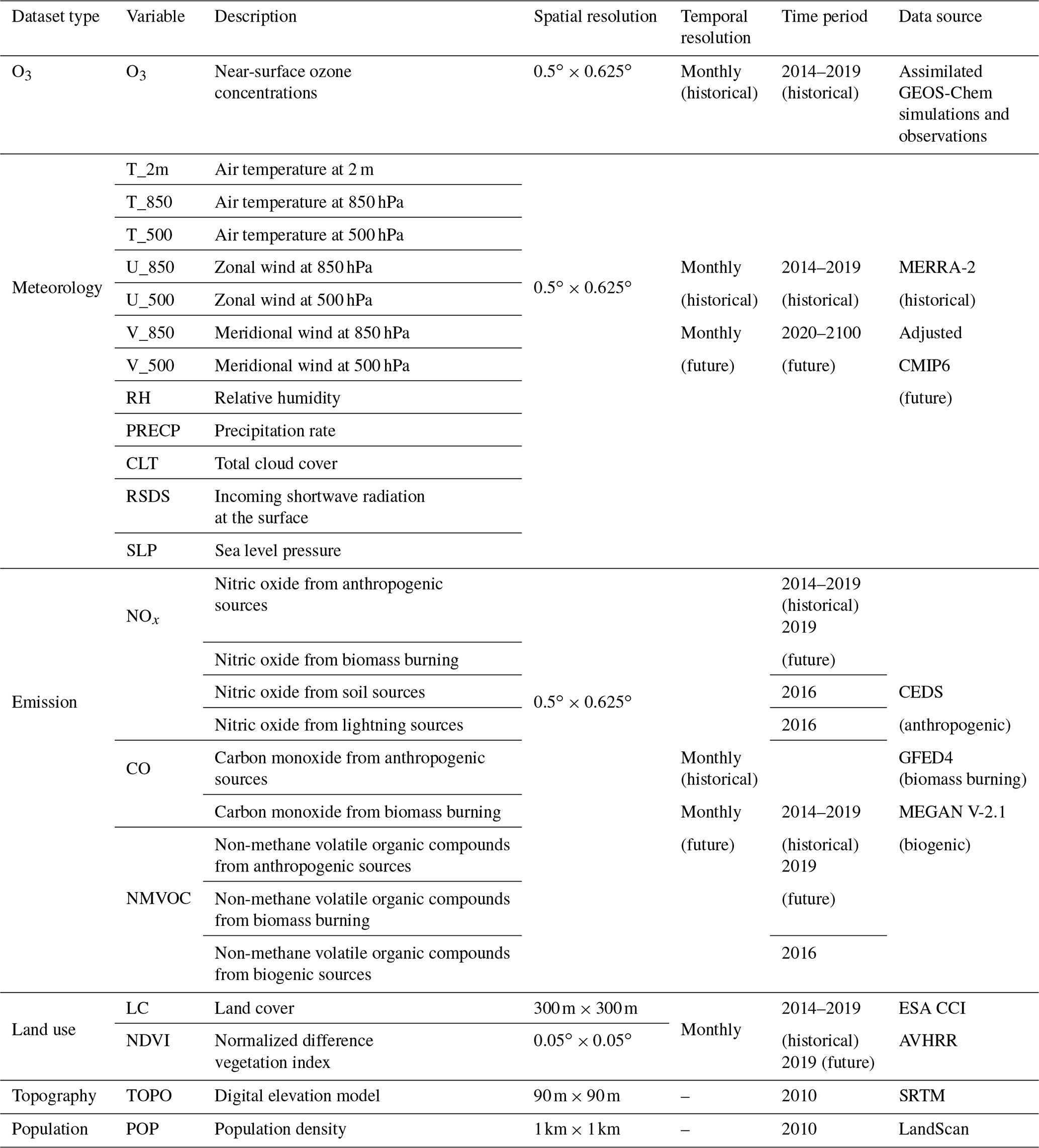
Table 1Summary of detailed datasets used in this study. AVHRR: Advanced Very High Resolution Radiometer; ESA CCI: ESA Climate Change Initiative; SRTM: Shuttle Radar Topography Mission.
2.4 Predicting O3 using a machine learning method
In this study, a random forest (RF) model is used to predict O3 concentrations, similar to our previous studies (H. Li et al., 2021, 2022), with input data of assimilated O3 concentrations in China that combine observations and results from GEOS-Chem model simulations, GEOS-Chem simulated O3 concentrations outside of China, MERRA-2 meteorological variables, O3 precursor emissions, land cover (LC), the normalized difference vegetation index (NDVI), topography (TOPO), population density (POP), the month of the year (MOY), and the geographic location of each model grid as spatiotemporal information. Details of the datasets are summarized in Table 1.
For predicting future climate-driven near-surface O3 concentrations, the ML model is trained with samples over 2014–2018 and the remaining 2019 data are used for model validation. To obtain an optimal ML model, hyperparameters are firstly tuned using the 10-fold cross-validation (Rodriguez et al., 2010). The best hyperparameters (n_estimators =200, min_samples_split =2, max_features = “sqrt”, bootstrap = “True”) of the ML model are utilized. Several statistical metrics, including the coefficient of determination (R2), mean absolute error (MAE), root mean square error (RMSE), and mean relative error (MRE), are used to evaluate the performance of ML model. Then the climate-driven near-surface O3 concentrations during 2020–2100 under four SSPs (SSP1-2.6, SSP2-4.5, SSP3-7.0, and SSP5-8.5) in Asia can be estimated using the trained ML model with varying meteorological factors under the climate change scenarios. Both anthropogenic and natural emissions of O3 precursors are fixed at the present-day levels for the prediction.
2.5 Meteorological fields from CMIP6 multi-model simulations
Monthly meteorological parameters under four different future climate scenarios, including SSP1-2.6, SSP2-4.5, SSP3-7.0, and SSP5-8.5 (a representation of low-, intermediate-, medium–high-, and high-forcing levels, respectively), are fed to an ML model to predict near-surface O3 concentrations. The Scenario Model Intercomparison Project (ScenarioMIP) as part of CMIP6 provides multi-model projections of climate variables driven by future emission and land use changes under different SSPs (O'Neill et al., 2016). In our study, meteorological fields, such as air temperature (at 2 m, 850 hPa, and 500 hPa), wind fields (at 850 and 500 hPa), surface relative humidity, incoming shortwave radiation at the surface, total cloud cover, precipitation rate, and sea level pressure, are chosen as the key meteorological predictors for near-surface O3 concentrations, which are obtained from 18 global climate models, i.e., ACCESS-CM2, ACCESS-ESM1-5, CanESM5, CESM2-WACCM, CMCC-CM2-SR5, EC-Earth3-Veg, EC-Earth3, FGOALS-f3-L, FGOALS-g3, GFDL-ESM4, INM-CM5-0, IPSL-CM6A-LR, MIROC6, MPI-ESM1-2-HR, MPI-ESM1-2-LR, MRI-ESM2-0, NorESM2-LM, and NorESM2-MM. Before being applied to the ML model, future meteorological fields from ScenarioMIP are adjusted by their potential bias, characterized as the difference in their historical climatological mean (2014–2019) and MERRA-2 following Li et al. (2022). It minimizes the inconsistencies in the initial conditions in models and reanalysis data.
3.1 Predictive capability of the machine learning model
The predicted monthly O3 concentrations over Asia in 2019 by the ML model are in good agreement with the assimilated O3 data constructed with observations and GEOS-Chem model results (Fig. 3). The overall R2 between the predicted and assimilated O3 concentrations is as high as 0.92, and the ML model has a low MRE of 9 % in predicting O3 concentrations over the Asia domain. Overall, these statistical indices indicate that the RF model is promising for predicting the spatial distributions and temporal variations in near-surface O3 concentrations over Asia, which can provide a practical means for studying long-term variations in O3 under the future climate change.
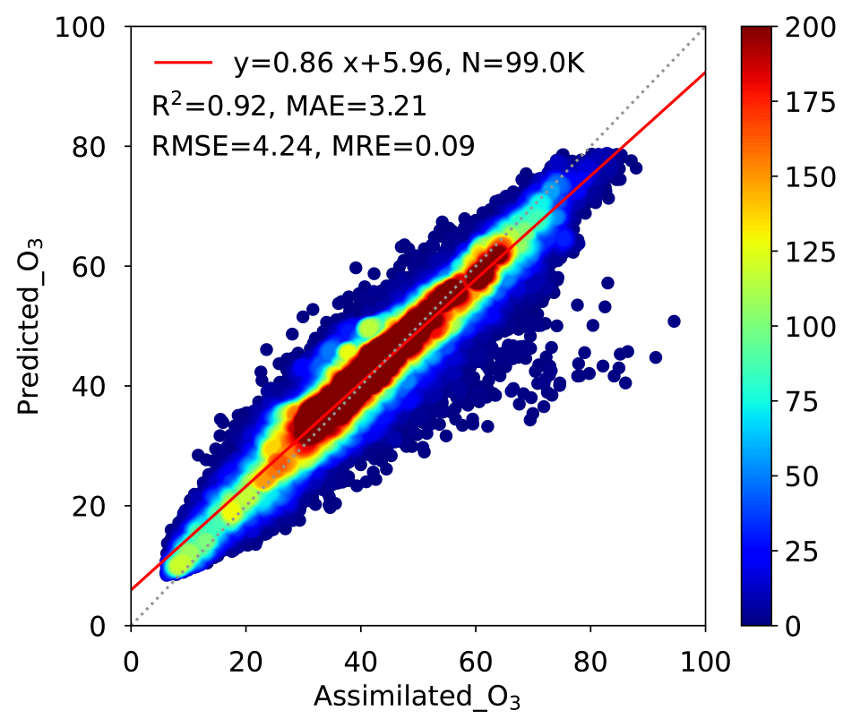
Figure 3Density scatterplots of predicted vs. assimilated monthly near-surface O3 concentrations (ppb) in 2019 over Asia. The gray and red lines are the 1:1 line and linear regression line, respectively. Statistical metrics including the number of samples (N), correlation of determination (R2, unitless), root mean square error (RMSE, ppb), mean absolute error (MAE, ppb), and mean relative error (MRE, %) are shown at the top left.
Meanwhile, the ML model predictive capability for each grid cell over the entire domain during 2014–2019 is further evaluated and demonstrated in Fig. 4. Regarding the spatial performance, the estimated O3 concentrations are highly correlated to the assimilated data in most regions of Asia with small biases, indicating a strong spatial predictive ability of the RF model. More than 80 % of land areas have an R2 greater than 0.9. In terms of model uncertainties, about 95 % of land areas have an RMSE (MAE) of less than 3 ppb (2 ppb) (parts per billion). Furthermore, approximately 86 % of land areas show small modeling bias with MRE below 5 %. Note that several grid cells show MRE over 5 % but still below 15 %, which is related to the data assimilation using monitored and simulated O3 concentrations in China and the coarse resolution for coastal areas and islands over Southeast Asia.
Figure 5 shows the importance score of independent variables that contribute to the prediction of the trained ML model, which called Gini importance and implies the influence of input features on the target variable in the ML model. The results suggest that among all the input predictors, relative humidity, incoming solar radiation at the surface, and topography are the top-three most influential variables for the model construction of near-surface O3 in Asia, with importance scores of 15 %, 12 %, and 10 %, respectively. The primary importance of relative humidity has also been reported in previous studies (e.g., Han et al., 2020; Qian et al., 2022). Other meteorological parameters, such as cloud cover, sea level pressure, air temperature, and precipitation, also have a substantial impact on the O3 estimates, with importance scores ranging from 4 % to 8 %. In the ML model, the emissions of three primary O3 precursors, including NMVOCs, NOx, and CO, have a relatively low importance score of 4 %–5 % individually due to the spatiotemporal diversity of O3 production regimes. However, it is noted that the O3 variations in different regions are dominated by different meteorological factors (Weng et al., 2022). The importance score of each independent feature quantified in this study can only reflect the overall importance across Asia, which is less representative of any specific regions.
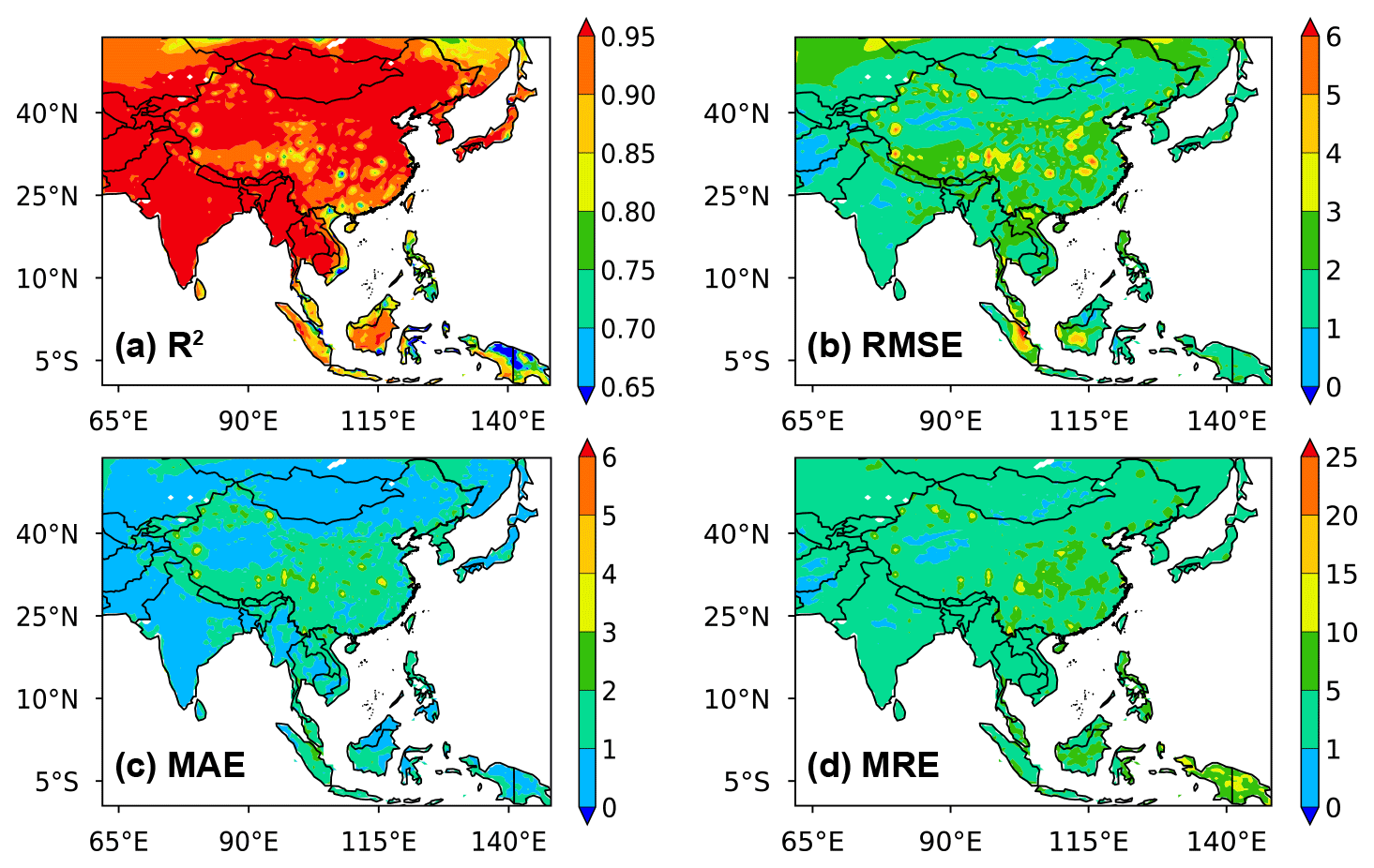
Figure 4Spatial distributions of the performance statistics of the ML model with regard to (a) R2 (unitless), (b) RMSE (ppb), (c) MAE (ppb), and (d) MRE (%) during 2014–2019 over Asia.
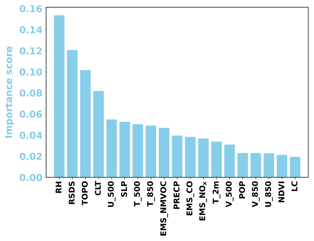
Figure 5Importance scores of independent variables (meteorological parameters, emissions, land use, topography, and population density) used in the ML model for predicting future near-surface O3 concentrations over Asia.
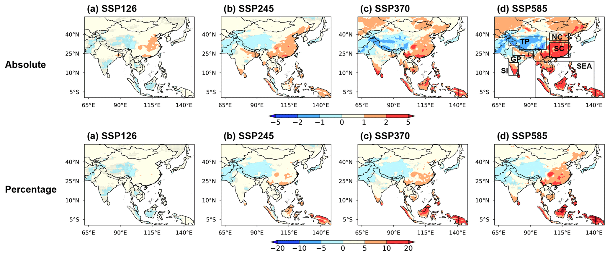
Figure 6The spatial distributions of absolute (ppb) and percentage difference (%) of surface O3 level between 2025 (2020–2029 mean) and 2095 (2091–2100 mean) driven by climate change under four scenarios (a, e) SSP1-2.6 (SSP126), (b, f) SSP2-4.5 (SSP245), (c, g) SSP3-7.0 (SSP370), and (d, h) SSP5-8.5 (SSP585). The box-outlined areas in (d) are North China (NC; 35–41∘ N, 105–120∘ E), South China (SC; 22–33.5∘ N, 105–120∘ E), Southeast Asia (SEA; 9.5∘ S–19∘ N, 93.75–140∘ E), South India (SI; 8–18∘ N, 73.125–80.625∘ E), the Gangetic Plains (GP; 21.5–23.5∘ N, 85.625–92.5∘ E; 23.5–27∘ N, 76.25–92.5∘ E; and 27–30∘ N, 76.25—81.25∘ E), and the Tibetan Plateau (TP; 28–31∘ N, 81.875–102.5∘ E and 31–38∘ N, 73.125–102.5∘ E). No overlaying hatch pattern indicates statistical significance with 95 % confidence from a two-tailed t test.
3.2 Predicted future climate-driven O3 variations
Figure 6 shows the predicted absolute and percentage changes in annual mean near-surface O3 concentrations in response to climate change between the first and last decades of 2020–2100 based on the future meteorological fields from the 18 CMIP6 models. Figure 7 shows the time series of the regional averaged values over six sub-regions of Asia during 2020–2100. Under the global warming trends of all future scenarios, the climate-driven near-surface O3 concentrations increase constantly from 2020 to 2100 over many key regions in Asia, such as North China (NC), South China (SC), Southeast Asia (SEA), South India (SI), and the Gangetic Plains (GP), except the Tibetan Plateau (TP). The O3 concentrations over SC, SEA, and SI are projected to increase considerably with the maximum increase up to 5 ppb (20 %) in 2095 (2091–2100 mean) compared to 2025 (2020–2029 mean) under the SSP5-8.5 scenario, revealing a strong O3–climate penalty in most Asian regions. The climate-driven changes in O3 concentrations are smaller under the scenarios of less warming, especially in SSP1-2.6 that has O3 changes of less than 5 % across Asia. These suggest that future climate following low emissions and sustainable pathways is more favorable for the mitigation of O3 pollution in Asia than high-forcing scenarios.
The strong O3–climate penalty over eastern China can be attributed to the particularly high O3 precursor emissions (Fig. S1 in the Supplement), relative to western China, which lead to a positive local net O3 production close to sources in a warming climate (Fig. S2) (Zanis et al., 2022). The absolute and percentage changes in regional averaged near-surface O3 concentrations between 2025 and 2095 under the four scenarios are shown in Fig. 8. The climate-driven changes in O3 concentrations are gradually stronger from the north (2 %–3 %) to the south (3 %–8 %) of China, which demonstrates that the changes in meteorology exert a greater impact on near-surface O3 concentrations over SC than NC under future climate change. By the end of the 21st century, the relative humidity will decrease (Fig. S3) and downward solar radiation will increase (Fig. S4) over SC compared to those values in 2025, which are conducive to the O3 productions, while NC has the opposite changes. Moreover, cloud cover will decrease more over SC than NC (Fig. S5), contributing to the larger increase in O3 productions and concentrations over SC than NC in a warming climate.
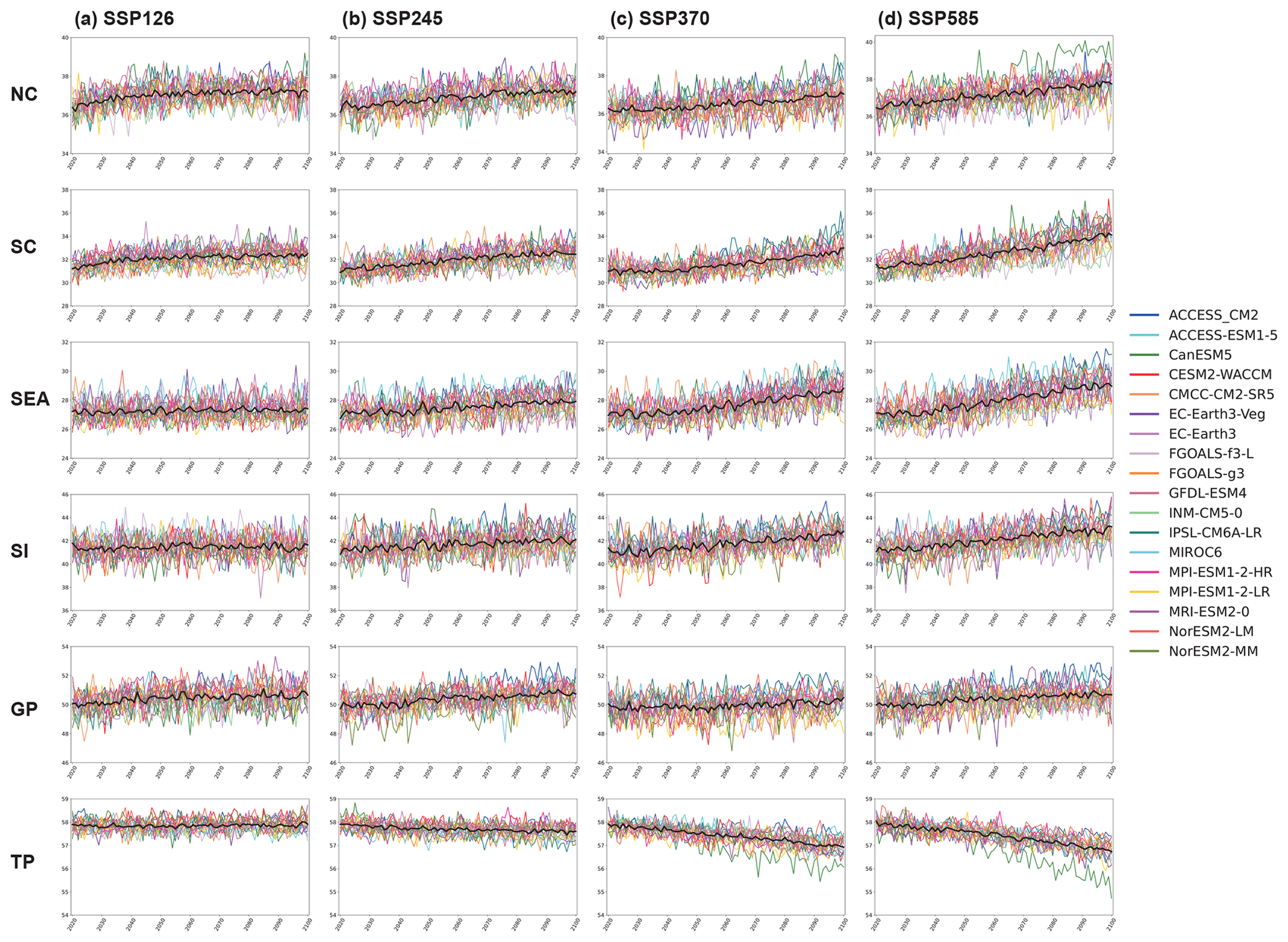
Figure 7Time series (2020–2100) of annual mean near-surface O3 concentrations (ppb) driven by climate change under the four scenarios (SSP1-2.6, SSP2-4.5, SSP3-7.0, and SSP5-8.5) over North China (NC; 35–41∘ N, 105–120∘ E), South China (SC; 22–33.5∘ N, 105–120∘ E), Southeast Asia (SEA; 9.5∘ S–19∘ N, 93.75–140∘ E), South India (SI; 8–18∘ N, 73.125–80.625∘ E), the Gangetic Plains (GP; 21.5–23.5∘ N, 85.625–92.5∘ E; 23.5–27∘ N, 76.25–92.5∘ E; and 27–30∘ N, 76.25–81.25∘ E), and the Tibetan Plateau (TP; 28–31∘ N, 81.875–102.5∘ E and 31–38∘ N, 73.125–102.5∘ E). The black lines are the averages of the predicted O3 based on meteorological fields from 18 CMIP6 models.
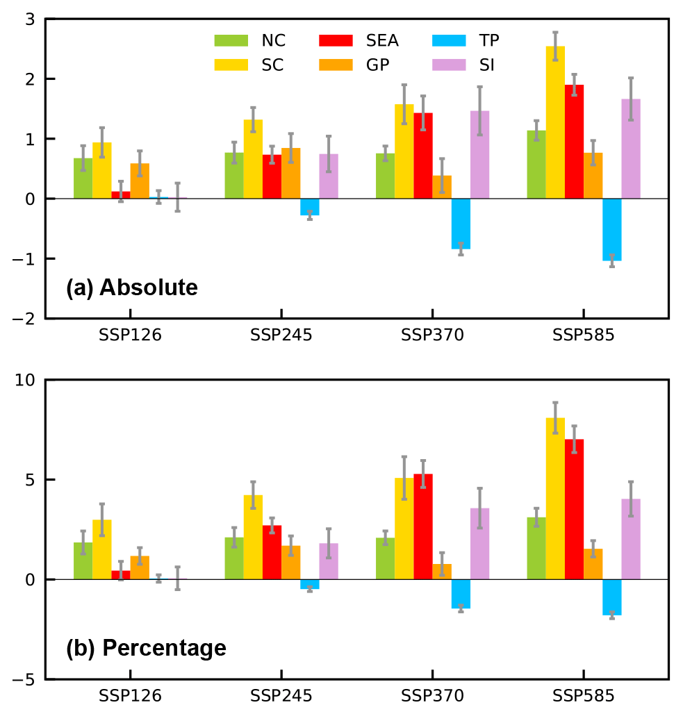
Figure 8Absolute (a, ppb) and percentage (b, %) changes in projected near-surface climate-driven O3 concentrations in 2095 (2091–2100 mean) relative to 2025 (2020–2029 mean) over the six selected key regions of Asia, including NC, SC, SEA, SI, GP, and TP under four future climate scenarios. The error bars indicate 1 standard deviation.
In South Asia, climate change also enhances O3 concentrations by <5 % over GP and SI (Fig. 8), due to the massive precursor emissions (Fig. S1) and O3 productions. Over SI, the decreases in relative humidity (Fig. S3) and cloud amount (Fig. S5) and increases in downward solar radiation at the surface (Fig. S4) favor photochemical production of O3 and induce the large increases in O3 concentrations in this region. Averaged over SEA, O3 concentrations driven by higher temperature (Fig. S2), more downward solar radiation (Fig. S4), and lower relative humidity (Fig. S3) and cloud cover (Fig. S5) in 2095 are projected to increase O3 concentrations by 5 %–7 % in SSP3-7.0 and SSP5-8.5 and 0 %–3 % in SSP1-2.6 and SSP2-4.5 scenarios, relative to 2025 (Fig. 8).
The Tibetan Plateau (TP), known as the highest topography in China with more solar radiation at the surface, has strong stratosphere–troposphere exchanges of O3 compared with other regions, leading to high O3 concentrations over this region (Fig. S6). Climate-driven O3 concentrations are projected to decline by less than 2 % over TP from 2025 to 2095 (Fig. 8). It is likely because less solar radiation (Fig. S4) and more frequent occurrence of rainy weather (Fig. S7) in the future would reduce the local chemical production of O3.
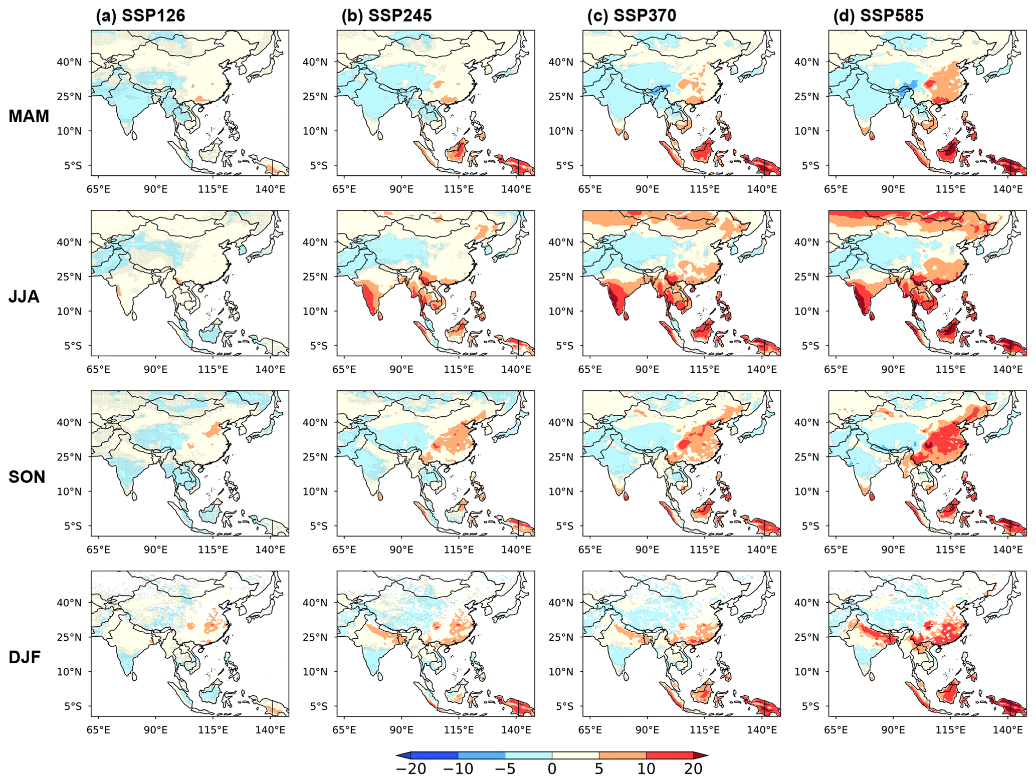
Figure 9The spatial distributions of percentage differences (%) in near-surface O3 concentrations between 2025 (2020–2029 mean) and 2095 (2091–2100 mean) driven by climate change under four scenarios (SSP1-2.6, SSP2-4.5, SSP3-7.0, and SSP5-8.5, from left to right) averaged in MAM (March–April–May), JJA (June–July–August), SON (September–October–November), and DJF (December–January–February) (from top to bottom). No overlaying hatch pattern indicates statistical significance with 95 % confidence from a two-tailed t test.
3.3 The seasonality of future climate-driven O3 variations
Climate over Asia has obvious seasonal variation related to the Asian monsoon system. Figure 9 shows the spatial distributions of percentage changes in projected climate-driven O3 concentrations in spring (March–April–May, MAM), summer (June–July–August, JJA), autumn (September–October–November, SON), and winter (December–January–February, DJF) between 2025 and 2095 under the four scenarios. In general, air quality in many regions of Asia will deteriorate in all seasons associated with intensified O3 pollution under climate change.
In eastern China, O3 pollution occurs most frequently in summer and is more severe in NC than SC currently (Li et al., 2019). Under future climate warming, JJA O3 concentrations will increase by 5 %–20 % in SC under the high-forcing scenarios, while the changes in NC are less than 5 %. This suggests that future climate change will expand the summertime O3 pollution from NC to SC over eastern China. Another feature is the strong increases in O3 concentrations by 10 %–20 % throughout eastern China and exceeding 20 % over Sichuan Basin in SON, which relate to the significant increases in temperature (Fig. S8) and solar radiation (Fig. S9) in this season over central-eastern China under the high-forcing scenarios. It further indicates that future climate change will extend the O3 pollution from summer into autumn.
In South Asia, the climate-driven increases in O3 concentrations vary from JJA over SI to DJF over GP. Relative to 2025, in the summer of 2095, anomalous high pressure (Fig. S10) along with an anticyclone (Figs. S11 and S12) dominates South Asia, which is not conducive to O3 diffusion, leading to increases in JJA O3 concentrations over SI. The intensified O3 pollution across GP in DJF under climate change is related to the strong surface warming (Fig. S8), decreases in relative humidity (Fig. S13), cloud cover (Fig. S14), and rainfall (Fig. S15), as well as increases in solar radiation at the surface (Fig. S9), favoring the photochemical production of O3. In the northern part of Southeast Asia, JJA has the largest O3 rise via the same mechanism as SI, while O3 increases by the same magnitude in all seasons in the southern part of Southeast Asia driven by future climate change.
O3 pollution has been increasing over Asia in recent decades, which harms human health and vegetation. In the future warmer climate, O3 pollution over Asia can be modulated by changes in meteorological fields. In this study, to examine the variations in O3 concentrations over Asia due to the future climate change, monthly near-surface O3 concentrations from 2020 to 2100 under four climate scenarios (SSP1-2.6, SSP2-4.5, SSP3-7.0, and SSP5-8.5) are predicted using an ML model with input data from assimilated O3 combining GEOS-Chem simulations and real-time observations, future meteorological parameters from CMIP6 multi-model simulations, emissions of O3 precursors, land use, topography, population density, and spatiotemporal information. Our results suggest that future O3 pollution over Asia will be significantly exacerbated in a warming climate, especially under high-forcing scenarios.
Trained by the assimilated O3 concentrations and reanalysis data, the ML model can well predict O3 over Asia with the coefficient determination of 0.92 between assimilated and predicted O3 concentrations and relative error of 9 %. Then the future Asian O3 concentrations from 2020 to 2100 driven by climate change are projected in the ML model with varying meteorological fields from 18 CMIP6 models under four future climate scenarios.
The climate penalty on O3 is robust over most regions of Asia. The annual mean O3 levels in 2095 are projected to increase by 5 %–20 % relative to 2025 under the high-forcing scenarios over South China, Southeast Asia, and South India and less than 10 % over North China and the Gangetic Plains, due to more favorable meteorological conditions for O3 photochemical production, while there is a decrease of <5 % over the Tibetan Plateau. The climate-driven changes in O3 concentrations are smaller under the scenarios of less warming, suggesting that future climate following low emissions and sustainable pathways would be more effective in the mitigation of O3 pollution in Asia than the high-forcing scenarios. Seasonal variation analysis reveals that summertime O3 pollution over eastern China will expand from North China to South China and extend into the cold season under future climate change. In addition, South Asian O3 pollution will increase over South India in summer and over the Gangetic Plains in winter.
Zanis et al. (2022) analyzed the global climate change benefit and penalty of O3 based on sensitivity simulations from five CMIP6 models under the SSP3-7.0 scenario. They showed positive changes in JJA O3 concentrations by less than 1 ppb from 2010 to 2095 over East Asia and South Asia driven by climate change but with large uncertainties due to the model diversity. The ML method in this study gives similar positive changes in O3 as Zanis et al. (2022). Pommier et al. (2018) applied the EMEP (European Monitoring and Evaluation Programme) chemical transport model driven by the downscaled meteorological data from NorESM1-M to investigate the impacts of regional climate change on near-surface O3 over India. They showed that near-surface O3 would increase by up to 4 % over northern India and decrease by 3 % over southern India from 2050 to 2100 under the RCP8.5 scenario. We show that the climate-driven O3 in this study would increase over both the Gangetic Plains (0.2 %) and South India (3 %) under the SSP5-8.5 scenario in 2050 relative to 2016 (2014–2019 mean). The discrepancies may rise from that the results of Pommier et al. (2018) were based on NorESM1-M simulated climate alone, while the climate change predicted by 18 CMIP6 models were applied in this study and the ensemble mean O3 concentrations were shown here.
There are a few uncertainties and limitations in the projected near-surface O3 concentrations over Asia in terms of input data, GEOS-Chem simulations, CMIP6 multi-model simulations, and the ML model. First, only observational data over 2014–2019 across China were used for the O3 assimilation. Longer-term measurements with broader spatial coverage are more desirable to improve the model performance. Land use data and population density are fixed at present-day conditions when predicting the future O3 since we focus on the variations in meteorological parameters under climate change, which will vary in the future. In addition, natural O3 precursor emissions such as biogenic emissions of NMVOCs and NOx from soil and lightning sources are fixed at levels from the year 2016 in the future estimates, which can induce biases in the O3 projections since climate change can strongly influence natural emissions of O3 precursors (Liu et al., 2019). Although the methane concentrations in the GEOS-Chem model are prescribed and its role in the O3 production is not considered in the ML model, the climate influence of methane is included in the CMIP6 multi-model simulations. Consequently, the impact of future changes in methane on O3 concentrations via climate change are considered in the future projections.
Second, the GEOS-Chem model has been demonstrated to well capture the magnitude of and spatiotemporal variations in O3, with an average bias of about 10 % over China (Lou et al., 2014) and Southeast Asia (Marvin et al., 2021) and less than 20 % over India (David et al., 2019). The future decrease in relative humidity will cause stomatal closure and also increase near-surface O3. The O3–vegetation interactions are not represented in the default GEOS-Chem model. A newly coupled global atmospheric chemistry–vegetation model (Lei et al., 2020) could be applied in the future study.
Third, the meteorological parameters characterizing future climate change from the CMIP6 multi-model simulations can also give rise to uncertainties in this study (Xu et al., 2021). Moreover, the spatial autocorrelation in a random split of training data for cross-validation would lead to the overly optimistic statistics of ML model predictive power (Ploton et al., 2020). Additionally, the overall importance scores of the features in this study can only reflect that from the whole study domain. Further investigations are required to identify and quantify the importance score of each local variable contribution to the near-surface O3 predictions in different specific regions. Also, the good ability of the ML model for the present-day condition may not imply a satisfactorily extrapolation under the future warming condition, which can bias our results and deserves further investigation in future studies.
Last but not least, near-surface O3 has increased rapidly in China since 2013 owing to both precursor emission changes and atmospheric warming (Li et al., 2021b), which significantly affect human health (Lu et al., 2020) and also require further studies.
Overall, our study provides a framework of combining real-time observations, chemical transport model simulations, and multi-climate model predictions with data assimilation and machine learning methods to estimate future climate-driven near-surface O3 concentrations. The emphasis of this work is to quantify the impacts of future climate change on O3 pollution in Asia, which is of great significance for future O3 pollution mitigation strategies.
The GEOS-Chem model is available at https://doi.org/10.5281/zenodo.3974569 (The International GEOS-Chem User Community, 2020). MERRA-2 reanalysis data can be downloaded at http://geoschemdata.wustl.edu/ExtData/GEOS_0.5x0.625_AS/MERRA2/ (GMAO, 2020). Multi-model projections of climate variables are from the Scenario Model Intercomparison Project of the Coupled Model Intercomparison Project Phase 6 https://esgf-node.llnl.gov/search/cmip6/ (Coupled Model Intercomparison Project, 2020). Land cover is derived from http://maps.elie.ucl.ac.be/CCI/viewer/download.php (European Space Agency Climate Change Initiative, 2017). Hourly O3 concentrations are obtained from the public website of the China Ministry of Ecology and Environment (http://www.beijingair.sinaapp.com, Wang, 2020). The normalized difference vegetation index is obtained from https://www.ncei.noaa.gov/data/avhrr-land-normalized-difference-vegetation-index/access/ (NOAA National Centers for Environmental Information, 2019). Topography is collected from https://cgiarcsi.community/data/srtm-90m-digital-elevation-database-v4- (Jarvis et al., 2008). Population density is acquired from https://doi.org/10.48690/1524206 (Bright et al., 2011).
The supplement related to this article is available online at: https://doi.org/10.5194/acp-23-1131-2023-supplement.
YY designed the research. HL performed the model simulations, analyzed data, and wrote the initial draft. JJ designed the data assimilation. YY, JJ, HW, and KL helped edit and review the manuscript. All the authors discussed the results and contributed to the final manuscript.
The contact author has declared that none of the authors has any competing interests.
Publisher’s note: Copernicus Publications remains neutral with regard to jurisdictional claims in published maps and institutional affiliations.
Hailong Wang acknowledges the support by the U.S. Department of Energy (DOE) Office of Science's Biological and Environmental Research (BER) program as part of the Earth and Environmental System Modeling program. The Pacific Northwest National Laboratory (PNNL) is operated for DOE by the Battelle Memorial Institute (contract no. DE-AC05-76RLO1830). The projected O3 concentrations in this study are available upon request.
This study was supported by the National Natural Science Foundation of China (grant nos. 42293320 and 41975159), the National Key Research and Development Program of China (grant nos. 2019YFA0606800 and 2020YFA0607803), the Jiangsu Science Fund for Distinguished Young Scholars (grant no. BK20211541) and the Jiangsu Science Fund for Carbon Neutrality (grant no. BK20220031).
This paper was edited by Joshua Fu and reviewed by two anonymous referees.
Bey, I., Jacob, D. J., Yantosca, R. M., Logan, J. A., Field, B. D., Fiore, A. M., Li, Q., Liu, H., Mickley, L. J., and Schultz, M. G.: Global modeling of tropospheric chemistry with assimilated meteorology: Model description and evaluation, J. Geophys. Res.-Atmos., 106, 23073–23095, https://doi.org/10.1029/2001JD000807, 2001.
Bright, E., Coleman, P., Rose, A., and Urban, M.: LandScan Global 2010, Oak Ridge National Laboratory [data set], https://doi.org/10.48690/1524206, 2022.
Cakmak, S., Hebbern, C., Pinault, L., Lavigne, E., Vanos, J., Crouse, D. L., and Tjepkema, M.: Associations between long-term PM2.5 and ozone exposure and mortality in the Canadian Census Health and Environment Cohort (CANCHEC), by spatial synoptic classification zone, Environ. Int., 111, 200–211, https://doi.org/10.1016/j.envint.2017.11.030, 2018.
Checa-Garcia, R., Hegglin, M. I., Kinnison, D., Plummer, D. A., and Shine, K. P.: Historical tropospheric and stratospheric ozone radiative forcing using the CMIP6 database, Geophys. Res. Lett., 45, 3264–3273, https://doi.org/10.1002/2017GL076770, 2018.
Chen, L., Liang, S., Li, X., Mao, J., Gao, S., Zhang, H., Sun, Y., Vedal, S., Bai, Z., Ma, Z., Haiyu., and Azzi, M.: A hybrid approach to estimating long-term and short-term exposure levels of ozone at the national scale in China using land use regression and Bayesian maximum entropy, Sci. Total Environ., 752, 141780, https://doi.org/10.1016/j.scitotenv.2020.141780, 2020.
Cheng, J., Tong, D., Zhang, Q., Liu, Y., Lei, Y., Yan, G., Yan, L., Yu, S., Cui, R. Y., Clarke, L., Geng, G., Zheng, B., Zhang, X., Davis, S. J., and He, K.: Pathways of China's PM2.5 air quality 2015−2060 in the context of carbon neutrality, Natl. Sci. Rev., 8, nwab078, https://doi.org/10.1093/nsr/nwab078, 2021.
Colette, A., Andersson, C., Baklanov, A., Bessagnet, B., Brandt, J., Christensen, J. H., Doherty, R., Engardt, M., Geels, C., Giannakopoulos, C., Hedegaard, G. B., Katragkou, E., Langner, J., Lei, H., Manders, A., Melas, D., Meleux, F., Rouïl, L., Sofiev, M., Soares, J., Stevenson, D. S., Tombrou-Tzella, M., Varotsos, K. V., and Young, P.: Is the ozone climate penalty robust in Europe? Environ. Res. Lett., 10, 084015, https://doi.org/10.1088/1748-9326/10/8/084015, 2015.
Coupled Model Intercomparison Project: Scenario Model Intercomparison Project in Phase 6 [data set], https://esgf-node.llnl.gov/search/cmip6/, last access: 1 August 2022.
Dang, R., Liao, H., and Fu, Y.: Quantifying the anthropogenic and meteorological influences on summertime surface ozone in China over 2012–2017, Sci. Total Environ., 754, 142394, https://doi.org/10.1016/j.scitotenv.2020.142394, 2021.
David, L. M., Ravishankara, A., Brewer, J. F., Sauvage, B., Thouret, V., Venkataramani, S., and Sinha, V.: Tropospheric ozone over the Indian subcontinent from 2000 to 2015: Data set and simulation using GEOS-Chem chemical transport model, Atmos. Environ., 219, 117039, https://doi.org/10.1016/j.atmosenv.2019.117039, 2019.
Di, Q., Rowland, S., Koutrakis, P., and Schwartz, J.: A hybrid model for spatially and temporally resolved ozone exposures in the continental United States, J. Air Waste Manage., 67, 39–52, https://doi.org/10.1080/10962247.2016.1200159, 2017.
Doherty, R. M., Wild, O., Shindell, D. T., Zeng, G., MacKenzie, I. A., Collins, W. J., Fiore, A. M., Stevenson, D. S., Dentener, F. J., Schultz, M. G., Hess, P., Derwent, R. G., and Keating, T. J.: Impacts of climate change on surface ozone and intercontinental ozone pollution: A multi-model study, J. Geophys. Res., 118, 3744–3763, https://doi.org/10.1002/jgrd.50266, 2013.
European Space Agency Climate Change Initiative: Land cover classification [data set], http://maps.elie.ucl.ac.be/CCI/viewer/download.php, last access: 1 August 2022.
Evensen, G., Vossepoel, F. C., and van Leeuwen, P. J.: Data Assimilation Fundamentals: A Unified Formulation of the State and Parameter Estimation Problem, Springer Nature, https://doi.org/10.1007/978-3-030-96709-3, 2022.
Fann, N., Nolte, C. G., Dolwick, P., Spero, T. L., Brown, A. C., Phillips, S., and Anenberg, S.: The geographic distribution and economic value of climate change-related ozone health impacts in the United States in 2030, J. Air Waste Manage., 65, 570–580, https://doi.org/10.1080/10962247.2014.996270, 2015.
Fu, T.-M. and Tian, H.: Climate Change Penalty to Ozone Air Quality: Review of Current Understandings and Knowledge Gaps, Curr. Pollut. Rep., 5, 159–171, https://doi.org/10.1007/s40726-019-00115-6, 2019.
Fu, Y. and Tai, A. P. K.: Impact of climate and land cover changes on tropospheric ozone air quality and public health in East Asia between 1980 and 2010, Atmos. Chem. Phys., 15, 10093–10106, https://doi.org/10.5194/acp-15-10093-2015, 2015.
Gao, M., Gao, J., Zhu, B., Kumar, R., Lu, X., Song, S., Zhang, Y., Jia, B., Wang, P., Beig, G., Hu, J., Ying, Q., Zhang, H., Sherman, P., and McElroy, M. B.: Ozone pollution over China and India: seasonality and sources, Atmos. Chem. Phys., 20, 4399–4414, https://doi.org/10.5194/acp-20-4399-2020, 2020.
Gaudel, A., Cooper, O. R., Ancellet, G., Barret, B., Boynard, A., Burrows, J. P., Clerbaux, C., Coheur, P. F., Cuesta, J., Cuevas, E., Doniki, S., Dufour, G., Ebojie, F., Foret, G., Garcia, O., Granados-Muñoz, M. J., Hannigan, J. W., Hase, F., Hassler, B., Huang, G., Hurtmans, D., Jaffe, D., Jones, N., Kalabokas, P., Kerridge, B., Kulawik, S., Latter, B., Leblanc, T., Le Flochmoën, E., Lin, W., Liu, J., Liu, X., Mahieu, E., McClure-Begley, A., Neu, J. L., Osman, M., Palm, M., Petetin, H., Petropavlovskikh, I., Querel, R., Rahpoe, N., Rozanov, A., Schultz, M. G., Schwab, J., Siddans, R., Smale, D., Steinbacher, M., Tanimoto, H., Tarasick, D. W., Thouret, V., Thompson, A. M., Trickl, T., Weatherhead, E., Wespes, C., Worden, H. M., Vigouroux, C., Xu, X., Zeng, G., and Ziemke, J.: Tropospheric Ozone Assessment Report: Present-day distribution and trends of tropospheric ozone relevant to climate and global atmospheric chemistry model evaluation, Elem. Sci. Anth., 6, 39, https://doi.org/10.1525/elementa.291, 2018.
Gelaro, R., McCarty, W., Suárez, M. J., Todling, R., Molod, A., Takacs, L., Randles, C. A., Darmenov, A., Bosilovich, M. G., Reichle, R., Wargan, K., Coy, L., Cullather, R., Draper, C., Akella, S., Buchard, V., Conaty, A., da Silva, A. M., Gu, W., Kim, G.-K., Koster, R., Lucchesi, R., Merkova, D., Nielsen, J. E., Partyka, G., Pawson, S., Putman, W., Rienecker, M., Schubert, S. D., Sienkiewicz, M., and Zhao, B.: The Modern-Era Retrospective Analysis for Research and Applications, Version 2 (MERRA-2), J. Climate, 30, 5419–5454, https://doi.org/10.1175/JCLI-D-16-0758.1, 2017.
GMAO: Modern-Era Retrospective analysis for Research and Applications, Version 2 [data set], http://geoschemdata.wustl.edu/ExtData/GEOS_0.5x0.625_AS/MERRA2/, last access: 1 August 2022.
Gong, C. and Liao, H.: A typical weather pattern for ozone pollution events in North China, Atmos. Chem. Phys., 19, 13725–13740, https://doi.org/10.5194/acp-19-13725-2019, 2019.
Guenther, A. B., Jiang, X., Heald, C. L., Sakulyanontvittaya, T., Duhl, T., Emmons, L. K., and Wang, X.: The Model of Emissions of Gases and Aerosols from Nature version 2.1 (MEGAN2.1): an extended and updated framework for modeling biogenic emissions, Geosci. Model Dev., 5, 1471–1492, https://doi.org/10.5194/gmd-5-1471-2012, 2012.
Han, H., Liu, J., Shu, L., Wang, T., and Yuan, H.: Local and synoptic meteorological influences on daily variability in summertime surface ozone in eastern China, Atmos. Chem. Phys., 20, 203–222, https://doi.org/10.5194/acp-20-203-2020, 2020.
Hoesly, R. M., Smith, S. J., Feng, L., Klimont, Z., Janssens-Maenhout, G., Pitkanen, T., Seibert, J. J., Vu, L., Andres, R. J., Bolt, R. M., Bond, T. C., Dawidowski, L., Kholod, N., Kurokawa, J.-I., Li, M., Liu, L., Lu, Z., Moura, M. C. P., O'Rourke, P. R., and Zhang, Q.: Historical (1750–2014) anthropogenic emissions of reactive gases and aerosols from the Community Emissions Data System (CEDS), Geosci. Model Dev., 11, 369–408, https://doi.org/10.5194/gmd-11-369-2018, 2018.
Hudman, R. C., Moore, N. E., Mebust, A. K., Martin, R. V., Russell, A. R., Valin, L. C., and Cohen, R. C.: Steps towards a mechanistic model of global soil nitric oxide emissions: implementation and space based-constraints, Atmos. Chem. Phys., 12, 7779–7795, https://doi.org/10.5194/acp-12-7779-2012, 2012.
IPCC: Climate change 2021: The physical science basis. Contribution of working group I to the sixth assessment report of the intergovernmental panel on climate change, Cambridge, UK, Cambridge University Press, https://doi.org/10.1017/9781009157896, 2021.
Jacob, D. J. and Winner, D. A.: Effect of climate change on air quality, Atmos. Environ., 43, 51–63, https://doi.org/10.1016/j.atmosenv.2008.09.051, 2009.
Jarvis, A., Reuter, H. I., Nelson, A., and Guevara, E.: Hole-filled SRTM for the globe Version 4, available from the CGIAR-CSI SRTM 90m Database, https://cgiarcsi.community/data/srtm-90m-digital-elevation-database-v4-1, last access: 1 August 2022.
Jeong, J. I. and Park, R. J.: Effects of the meteorological variability on regional air quality in East Asia, Atmos. Environ., 69, 46–55, https://doi.org/10.1016/J.Atmosenv.2012.11.061, 2013.
Kalnay, E.: Atmospheric Modeling, Data Assimilation and Predictability, Cambridge University Press, Cambridge, UK, https://doi.org/10.1017/CBO9780511802270, 2003.
Kavassalis, S. C. and Murphy, J. G.: Understanding ozone-meteorology correlations: A role for dry deposition, Geophys. Res. Lett., 44, 2922–2931, https://doi.org/10.1002/2016gl071791, 2017.
Lei, Y., Yue, X., Liao, H., Gong, C., and Zhang, L.: Implementation of Yale Interactive terrestrial Biosphere model v1.0 into GEOS-Chem v12.0.0: a tool for biosphere–chemistry interactions, Geosci. Model Dev., 13, 1137–1153, https://doi.org/10.5194/gmd-13-1137-2020, 2020.
Li, H., Yang, Y., Wang, H., Li, B., Wang, P., Li, J., and Liao, H.: Constructing a spatiotemporally coherent long-term PM2.5 concentration dataset over China during 1980–2019 using a machine learning approach, Sci. Total Environ., 765, 144263, https://doi.org/10.1016/j.scitotenv.2020.144263, 2021.
Li, H., Yang, Y., Wang, H., Wang, P., Yue, X., and Liao, H.: Projected Aerosol Changes Driven by Emissions and Climate Change Using a Machine Learning Method, Environ. Sci. Technol., 56, 3884–3893, https://doi.org/10.1021/acs.est.1c04380, 2022.
Li, K., Jacob, D. J., Liao, H., Shen, L., Zhang, Q., and Bates, K. H.: Anthropogenic Drivers of 2013–2017 Trends in Summer Surface Ozone in China, P. Natl. Acad. Sci. USA, 116, 422–427, https://doi.org/10.1073/pnas.1812168116, 2019.
Li, K., Jacob, D. J., Shen, L., Lu, X., De Smedt, I., and Liao, H.: Increases in surface ozone pollution in China from 2013 to 2019: anthropogenic and meteorological influences, Atmos. Chem. Phys., 20, 11423–11433, https://doi.org/10.5194/acp-20-11423-2020, 2020.
Li, K., Jacob, D. J., Liao, H., Qiu, Y., Shen, L., Zhai, S., Bates, K. H., Sulprizio, M. P., Song, S., Lu, X., Zhang, Q., Zheng, B., Zhang, Y., Zhang, J., Lee, H. C., and Kuk, S. K.: Ozone pollution in the North China Plain spreading into the late-winter haze season, P. Natl. Acad. Sci. USA, 118, 1–7, https://doi.org/10.1073/pnas.2015797118, 2021.
Li, M., Yu, S., Chen, X., Li, Z., Zhang, Y., Wang, L., Liu, W., Li, P., Lichtfouse, E., Rosenfeld, D., and Seinfeld, J. H.: Large scale control of surface ozone by relative humidity observed during warm seasons in China, Environ. Chem. Lett., 19, 3981–3989, https://doi.org/10.1007/s10311-021-01265-0, 2021a.
Li, M., Wang, T., Shu, L., Qu, Y., Xie, M., Liu, J., Wu, H., and Kalsoom, U.: Rising surface ozone in China from 2013 to 2017: A response to the recent atmospheric warming or pollutant controls?, Atmos. Environ., 246, 118130, https://doi.org/10.1016/j.atmosenv.2020.118130, 2021b.
Lin, J.-T. and McElroy, M. B.: Impacts of boundary layer mixing on pollutant vertical profiles in the lower troposphere: Implications to satellite remote sensing, Atmos. Environ., 44, 1726–1739, https://doi.org/10.1016/j.atmosenv.2010.02.009, 2010.
Liu, R., Ma, Z., Liu, Y., Shao, Y., Zhao, W., and Bi, J.: Spatiotemporal distributions of surface ozone levels in China from 2005 to 2017: a machine learning approach, Environ. Int., 142, 105823, https://doi.org/10.1016/j.envint.2020.105823, 2020.
Liu, S., Xing, J., Zhang, H., Ding, D., Zhang, F., Zhao, B., Sahu, S. K., and Wang, S.: Climate-driven trends of biogenic volatile organic compound emissions and their impacts on summertime ozone and secondary organic aerosol in China in the 2050s, Atmos. Environ., 218, 117020, https://doi.org/10.1016/j.atmosenv.2019.117020, 2019.
Liu, X., Zhu, Y., Xue, L., Desai, A. R., and Wang, H.: Cluster-enhanced ensemble learning for mapping global monthly surface ozone from 2003 to 2019, Geophys. Res. Lett., 49, e2022GL097947, https://doi.org/10.1029/2022GL097947, 2022.
Liu, Y. and Wang, T.: Worsening urban ozone pollution in China from 2013 to 2017 – Part 1: The complex and varying roles of meteorology, Atmos. Chem. Phys., 20, 6305–6321, https://doi.org/10.5194/acp-20-6305-2020, 2020.
Lou, S., Liao, H., and Zhu, B.: Impacts of aerosols on surface-layer ozone concentrations in China through heterogeneous reactions and changes in photolysis rates, Atmos. Environ., 85, 123–138, https://doi.org/10.1016/j.atmosenv.2013.12.004, 2014.
Lu, X., Zhang, L., Chen, Y., Zhou, M., Zheng, B., Li, K., Liu, Y., Lin, J., Fu, T.-M., and Zhang, Q.: Exploring 2016–2017 surface ozone pollution over China: source contributions and meteorological influences, Atmos. Chem. Phys., 19, 8339–8361, https://doi.org/10.5194/acp-19-8339-2019, 2019.
Lu, X., Zhang, L., Wang, X., Gao, M., Li, K., Zhang, Y., Yue, X., and Zhang, Y.: Rapid Increases in Warm-Season Surface Ozone and Resulting Health Impact in China since 2013, Environ. Sci. Tech. Lett., 7, 240–247, https://doi.org/10.1021/acs.estlett.0c00171, 2020.
Malley, C. S., Henze, D. K., Kuylenstierna, J. C. I., Vallack, H., Davila, Y., Anenberg, S. C., Turner, M. C., and Ashmore, M.: Updated Global Estimates of Respiratory Mortality in Adults ≥ 30 Years of Age Attributable to Long-Term Ozone Exposure, Environ. Health Persp., 125, 087021, https://doi.org/10.1289/EHP1390, 2017.
Mao, J., Paulot, F., Jacob, D. J., Cohen, R. C., Crounse, J. D., Wennberg, P. O., Keller, C. A., Hudman, R. C., Barkley, M. P., and Horowitz, L. W.: Ozone and organic nitrates over the eastern United States: sensitivity to isoprene chemistry, J. Geophys. Res.-Atmos, 118, 11256–68, https://doi.org/10.1002/jgrd.50817, 2013.
Marvin, M. R., Palmer, P. I., Latter, B. G., Siddans, R., Kerridge, B. J., Latif, M. T., and Khan, M. F.: Photochemical environment over Southeast Asia primed for hazardous ozone levels with influx of nitrogen oxides from seasonal biomass burning, Atmos. Chem. Phys., 21, 1917–1935, https://doi.org/10.5194/acp-21-1917-2021, 2021.
McLinden, C. A., Olsen, S. C., Hannegan, B., Wild, O., Prather, M. J., and Sundet, J.: Stratospheric ozone in 3-D models: A simple chemistry and the cross-tropopause flux, J. Geophys. Res.-Atmos., 105, 14653–14665, https://doi.org/10.1029/2000jd900124, 2000.
Mills, G., Pleijel, H., Malley, C. S., Sinha, B., Cooper, O. R., Schultz, M. G., Neufeld, H. S., Simpson, D., Sharps, K., Feng, Z., Gerosa, G., Harmens, H., Kobayashi, K., Saxena, P., Paoletti, E., Sinha, V., and Xu, X.: Tropospheric ozone assessment report: Present-day tropospheric ozone distribution and trends relevant to vegetation, Elem. Sci. Anth., 6, 47, https://doi.org/10.1525/elementa.302, 2018.
Murray, L. T., Jacob, D. J., Logan, J. A., Hudman, R. C., and Koshak, W. J.: Optimized regional and interannual variability of lightning in a global chemical transport model constrained by LIS/OTD satellite data, J. Geophys. Res.-Atmos., 1117, D20307, https://doi.org/10.1029/2012jd017934, 2012.
Ni, R., Lin, J., Yan, Y., and Lin, W.: Foreign and domestic contributions to springtime ozone over China, Atmos. Chem. Phys., 18, 11447–11469, https://doi.org/10.5194/acp-18-11447-2018, 2018.
NOAA National Centers for Environmental Information: Normalized difference vegetation index [data set], https://www.ncei.noaa.gov/data/avhrr-land-normalized-difference-vegetation-index/access/, last access: 1 August 2022.
O'Neill, B. C., Tebaldi, C., van Vuuren, D. P., Eyring, V., Friedlingstein, P., Hurtt, G., Knutti, R., Kriegler, E., Lamarque, J.-F., Lowe, J., Meehl, G. A., Moss, R., Riahi, K., and Sanderson, B. M.: The Scenario Model Intercomparison Project (ScenarioMIP) for CMIP6, Geosci. Model Dev., 9, 3461–3482, https://doi.org/10.5194/gmd-9-3461-2016, 2016.
Ott, L. E., Pickering, K. E., Stenchikov, G. L., Allen, D. J., DeCaria, A. J., Ridley, B., Lin, R.-F., Lang, S., and Tao, W.-K.: Production of lightning NOx and its vertical distribution calculated from three-dimensional cloud-scale chemical transport model simulations, J. Geophys. Res., 115, D04301, https://doi.org/10.1029/2009JD011880, 2010.
Park, R. J., Jacob, D. J., Field, B. D., Yantosca, R. M., and Chin, M.: Natural and transboundary pollution influences on sulfate-nitrate-ammonium aerosols in the United States: Implications for policy, J. Geophys. Res.-Atmos., 109, D15204, https://doi.org/10.1029/2003jd004473, 2004.
Ploton, P., Mortier, F., Réjou-Méchain, M., Barbier, N., Picard, N., Rossi, V., Dormann, C., Cornu, G., Viennois, G., Bayol, N., Lyapustin, A., Gourlet-Fleury, S., and Pélissier, R.: Spatial validation reveals poor predictive performance of large-scale ecological mapping models, Nat. Commun., 11, 1–11, https://doi.org/10.1038/s41467-020-18321-y, 2020.
Pommier, M., Fagerli, H., Gauss, M., Simpson, D., Sharma, S., Sinha, V., Ghude, S. D., Landgren, O., Nyiri, A., and Wind, P.: Impact of regional climate change and future emission scenarios on surface O3 and PM2.5 over India, Atmos. Chem. Phys., 18, 103–127, https://doi.org/10.5194/acp-18-103-2018, 2018.
Pye, H. O. T., Liao, H., Wu, S., Mickley, L. J., Jacob, D. J., Henze, D. K., and Seinfeld, J. H.: Effect of changes in climate and emissions on future sulfate-nitrate-ammonium aerosol levels in the United States, J. Geophys. Res.-Atmos., 114, D01205, https://doi.org/10.1029/2008jd010701, 2009.
Qian, J., Liao, H., Yang, Y., Li, K., Chen, L., and Zhu, J.: Meteorological influences on daily variation and trend of summertime surface ozone over years of 2015–2020: Quantification for cities in the Yangtze River Delta, Sci. Total Environ., 834, 155107, https://doi.org/10.1016/j.scitotenv.2022.155107, 2022.
Rodriguez, J. D., Perez, A., and Lozano, J. A.: Sensitivity analysis of k-fold cross validation in prediction error estimation, IEEE T. Pattern Anal., 32, 569–575, https://doi.org/10.1109/TPAMI.2009.187, 2010.
Santurtún, A., González-Hidalgo, J. C., Sanchez-Lorenzo, A., and Zarrabeitia, M. T.: Surface ozone concentration trends and its relationship with weather types in Spain (2001–2010), Atmos. Environ., 101, 10–22, https://doi.org/10.1016/j.atmosenv.2014.11.005, 2015.
Su, X., An, J., Zhang, Y., Zhu, P., and Zhu, B.: Prediction of ozone hourly concentrations by support vector machine and kernel extreme learning machine using wavelet transformation and partial least squares methods, Atmos. Pollut. Res., 6, 51–60, https://doi.org/10.1016/j.apr.2020.02.024, 2020.
The International GEOS-Chem User Community: geoschem/geos-chem: GEOS-Chem 12.9.3 (12.9.3), Zenodo [code], https://doi.org/10.5281/zenodo.3974569, 2020.
Toh, Y. Y., Lim, S. F., and von Glasow, R.: The influence of meteorological factors and biomass burning on surface ozone concentrations at Tanah Rata, Malaysia, Atmos. Environ., 70, 435–446, https://doi.org/10.1016/j.atmosenv.2013.01.018, 2013.
van der Werf, G. R., Randerson, J. T., Giglio, L., van Leeuwen, T. T., Chen, Y., Rogers, B. M., Mu, M., van Marle, M. J. E., Morton, D. C., Collatz, G. J., Yokelson, R. J., and Kasibhatla, P. S.: Global fire emissions estimates during 1997–2016, Earth Syst. Sci. Data, 9, 697–720, https://doi.org/10.5194/essd-9-697-2017, 2017.
Wang, X.: Historical air quality data in China, https://quotsoft.net/air, last access: 1 August 2022.
Wang, Y., Shen, L., Wu, S., Mickley, L. J., He, J., and Hao, J.: Sensitivity of surface ozone over China to 2000–2050 global changes of climate and emissions, Atmos. Environ., 75, 374–382, https://doi.org/10.1016/j.atmosenv.2013.04.045, 2013.
Wang, Z., Lin, L., Xu, Y., Che, H., Zhang, X., Dong, W., Wang, C., Gui, K., and Xie, B.: Incorrect Asian aerosols affecting the attribution and projection of regional climate change in CMIP6 models, npj Clim. Atmos. Sci., 4, 2, https://doi.org/10.1038/s41612-020-00159-2, 2021.
Wei, J., Li, Z., Li, K., Dickerson, R., Pinker, R., Wang, J., Liu, X., Sun, L., Xue, W., and Cribb, M.: Full-coverage mapping and spatiotemporal variations of ground-level ozone (O3) pollution from 2013 to 2020 across China, Remote Sens. Environ., 270, 112775, https://doi.org/10.1016/j.rse.2021.112775, 2022.
Weng, X., Forster, G. L., and Nowack, P.: A machine learning approach to quantify meteorological drivers of ozone pollution in China from 2015 to 2019, Atmos. Chem. Phys., 22, 8385–8402, https://doi.org/10.5194/acp-22-8385-2022, 2022.
Xu, Z., Han, Y., Tam, C. Y., Yang, Z., and Fu, C.: Bias-corrected CMIP6 global dataset for dynamical downscaling of the historical and future climate (1979–2100), Sci. Data, 8, 293, https://doi.org/10.1038/s41597-021-01079-3, 2021.
Xue, T., Zheng, Y., Geng, G., Xiao, Q., Meng, X., Wang, M., Li, X., Wu, N., Zhang, Q., and Zhu, T.: Estimating Spatiotemporal Variation in Ambient Ozone Exposure during 2013–2017 Using a Data-Fusion Model, Environ. Sci. Technol., 54, 14877–14888, https://doi.org/10.1021/acs.est.0c03098, 2020.
Yang, Y., Li, M., Wang, H., Li, H., Wang, P., Li, K., Gao, M., and Liao, H.: ENSO modulation of summertime tropospheric ozone over China, Environ. Res. Lett., 17, 034020, https://doi.org/10.1088/1748-9326/ac54cd, 2022.
Yin, Z., Cao, B., and Wang, H.: Dominant patterns of summer ozone pollution in eastern China and associated atmospheric circulations, Atmos. Chem. Phys., 19, 13933–13943, https://doi.org/10.5194/acp-19-13933-2019, 2019.
Yue, X., Unger, N., Harper, K., Xia, X., Liao, H., Zhu, T., Xiao, J., Feng, Z., and Li, J.: Ozone and haze pollution weakens net primary productivity in China, Atmos. Chem. Phys., 17, 6073–6089, https://doi.org/10.5194/acp-17-6073-2017, 2017.
Zanis, P., Akritidis, D., Turnock, S., Naik, V., Szopa, S., Georgoulias, A. K., Bauer, S. E., Deushi, M., Horowitz, L. W., Keeble, J., Le Sager, P., O'Connor, F. M., Oshima, N., Tsigaridis, K., and van Noije., T.: Climate change penalty and benefit on surface ozone: a global perspective based on CMIP6 earth system models, Environ. Res. Lett., 17, 024014, https://doi.org/10.1088/1748-9326/ac4a34, 2022.
Zhang, X., Zhao, L., Cheng, M., and Chen, D.: Estimating ground-level ozone concentrations in eastern China using satellite-based precursors, IEEE T. Geosci. Remote, 58, 4754–4763, https://doi.org/10.1109/TGRS.2020.2966780, 2020.
Zhou, C., Gao, M., Li, J., Bai, K., Tang, X., Lu, X., Liu, C., Wang, Z., and Guo, Y.: Optimal Planning of Air Quality-Monitoring Sites for Better Depiction of PM2.5 Pollution across China, Environ. Au., 2, 314–323, https://doi.org/10.1021/acsenvironau.1c00051, 2022.
Zhu, J., Liao, H., Mao, Y., Yang, Y., and Jiang, H.: Interannual variation, decadal trend, and future change in ozone outflow from East Asia, Atmos. Chem. Phys., 17, 3729–3747, https://doi.org/10.5194/acp-17-3729-2017, 2017.