Sensitivities of cloud radiative effects to large-scale meteorology and aerosols from global observations

The radiative effects of clouds make a large contribution to the Earth's energy balance, and changes in clouds constitute the dominant source of uncertainty in the global warming response to carbon dioxide forcing. To characterize and constrain this uncertainty, cloud-controlling factor (CCF) analyses have been suggested that estimate sensitivities of clouds to large-scale environmental changes, typically in cloud-regime-specific multiple linear regression frameworks. Here, local sensitivities of cloud radiative effects to a large number of controlling factors are estimated in a regime-independent framework from 20 years (2001–2020) of near-global (60^∘ N–60^∘ S) satellite observations and reanalysis data using statistical learning. A regularized linear regression (ridge regression) is shown to skillfully predict anomalies of shortwave (R²=0.63) and longwave cloud radiative effects (CREs) (R²=0.72) in independent test data on the basis of 28 CCFs, including aerosol proxies. The sensitivity of CREs to selected CCFs is quantified and analyzed. CRE sensitivities to sea surface temperature and estimated inversion strength are particularly pronounced in low-cloud regions and generally in agreement with previous studies. The analysis of CRE sensitivities to three-dimensional wind field anomalies reflects the fact that CREs in tropical ascent regions are mainly driven by variability of large-scale vertical velocity in the upper troposphere. In the subtropics, CRE is sensitive to free-tropospheric zonal and meridional wind anomalies, which are likely to encapsulate information on synoptic variability that influences subtropical cloud systems by modifying wind shear and thus turbulence and dry-air entrainment in stratocumulus clouds, as well as variability related to midlatitude cyclones. Different proxies for aerosols are analyzed as CCFs, with satellite-derived aerosol proxies showing a larger CRE sensitivity than a proxy from an aerosol reanalysis, likely pointing to satellite aerosol retrieval biases close to clouds, leading to overestimated aerosol sensitivities. Sensitivities of shortwave CREs to all aerosol proxies indicate a pronounced cooling effect from aerosols in stratocumulus regions that is counteracted to a varying degree by a longwave warming effect. The analysis may guide the selection of CCFs in future sensitivity analyses aimed at constraining cloud feedback and climate forcings from aerosol–cloud interactions using data from both observations and global climate models.

1 Introduction

Clouds are main modulators of the Earth's energy budget, cooling the Earth by about 20 W m⁻² on average. This cooling is driven by clouds reflecting incoming shortwave solar radiation, therefore reducing the energy uptake of the Earth system by about 47 W m⁻². Clouds increase the Earth atmosphere's opacity in the infrared; however, they absorb longwave radiation emitted by the warmer Earth surface and emit less longwave radiation themselves due to the lower cloud-top temperatures. The combined effect of longwave absorption and emission leads to a warming of around 28 W m⁻² (numbers from Forster et al., 2021). These effects of clouds on the Earth's energy budget are called cloud radiative effects (CREs) and are defined as the difference in radiation between “all-sky” (cloudy and clear-sky) and (hypothetical) “clear-sky” conditions (Ramanathan et al., 1989). While shortwave CREs (CRE_SW) are mainly related to cloud fraction and microphysics (number concentration of water–ice particles and the amount of liquid water–ice), longwave CREs (CRE_LW) are mainly driven by cloud altitude and thus cloud-top temperature, but also cloud fraction (Voigt et al., 2021). As such, any change to cloud patterns, be it occurrence, microphysics, or macrostructure, has important implications for the Earth's energy balance. In a changing climate, clouds may be altered due to changes in the large-scale environment (cloud feedbacks) or due to a change in aerosol concentration (aerosol–cloud interactions, both are discussed below). In spite of their importance for the Earth's climate system, considerable uncertainty exists as to how clouds may respond to changes in their environmental controls, ultimately impeding the quantification of climate sensitivity, i.e., the global temperature increase following a doubling of the carbon dioxide (CO₂) concentration in the atmosphere compared to preindustrial levels (Zelinka et al., 2020; Forster et al., 2021).

Cloud feedbacks describe how clouds respond to and feed back on climate warming and are a major uncertainty in climate science. Many cloud feedbacks have been described in the literature, which relate changes in cloud altitude, phase, albedo, or coverage with global warming, typically in cloud-regime-specific frameworks (i.e., very few CCFs targeting a specific cloud type; e.g., Zelinka et al., 2016; Mülmenstädt et al., 2021; Murray et al., 2021; Zelinka et al., 2023). The most extensively studied shortwave cloud feedback is the (positive) low-cloud feedback (e.g., Klein et al., 2017; Scott et al., 2020; Myers et al., 2021; Cesana and Del Genio, 2021), which has been shown to be a main cause for the variation in climate sensitivity estimates in global climate models (Bony and Dufresne, 2005; Zelinka et al., 2020). The longwave or high-cloud feedback is also positive, where high clouds rise with warming temperatures, leading to a larger temperature differences between cloud top and the warming surface (Zelinka and Hartmann, 2010; Gettelman and Sherwood, 2016). Global satellite observations can help reduce the cloud-feedback-related uncertainty in climate sensitivity by constraining cloud feedbacks with observation-based sensitivity estimates of clouds (and their radiative effects) to changes in their large-scale environmental controls (cloud-controlling factors, CCFs). This is traditionally done in regime-specific cloud-controlling factor analyses, where cloud anomalies are regressed upon a small number of local CCF anomalies using an ordinary least-squares regression (OLS). Recently, a statistical learning framework (ridge regression), which allows for robust sensitivity estimation with many co-linear CCFs, has been used to predict cloudiness and constrain their feedbacks by using not only local CCF anomalies, but also their large-scale patterns (Andersen et al., 2020; Ceppi and Nowack, 2021). While regime-specific CCF frameworks are relatively well understood and thought to include the most relevant large-scale environmental controls of clouds in specific regimes (e.g., Klein et al., 2017), they do not necessarily include all relevant CCFs that may change in a warmer climate and thus influence the estimation of cloud feedbacks.

Atmospheric aerosols are another important driver of variability and trends in CREs (Quaas et al., 2022) because aerosols, by acting as cloud condensation nuclei (CCN), are drivers of cloud droplet number concentration in liquid water clouds. Under the assumption of a constant liquid water path, this leads to smaller cloud droplets and an increase in cloud reflectivity (Twomey, 1977). These instantaneous changes in cloud droplet characteristics may lead to the suppression or delay of precipitation, which in turn may trigger subsequent adjustments of the cloud field, such as an increase in cloud fraction or liquid water path (Albrecht, 1989), further altering CREs. Observational and modeling studies on the cloud fraction adjustment mostly find positive relationships (Kaufman and Koren, 2006; Gryspeerdt et al., 2016; Andersen et al., 2017; Christensen et al., 2020; Chen et al., 2022), while the sign of the liquid water path adjustment is still debated (Ackerman et al., 2004; Malavelle et al., 2017; Gryspeerdt et al., 2019; Rosenfeld et al., 2019; Toll et al., 2019; Manshausen et al., 2022; Zipfel et al., 2022; Wall et al., 2022). In convective cloud systems, a deepening or invigoration has been suggested; however, this effect is still elusive (Koren et al., 2005, 2010, 2014; Altaratz et al., 2014; Sarangi et al., 2018; Marinescu et al., 2021). Depending on the ambient air temperature, aerosols can also act as ice-nucleating particles, potentially increasing ice crystal number concentration and leading to further cloud adjustments (Hoose and Möhler, 2012; Gryspeerdt et al., 2018; Vergara-Temprado et al., 2018). The processes by which aerosols influence clouds depend on aerosol properties, ambient meteorology (dynamics and thermodynamics), and cloud regime (Stevens and Feingold, 2009; Andersen and Cermak, 2015; Andersen et al., 2016; Chen et al., 2016, 2018; Fuchs et al., 2018; Murray-Watson and Gryspeerdt, 2022; Zipfel et al., 2022). The effective radiative forcing due to aerosol–cloud interactions (i.e., the change in the Earth's net top-of-the-atmosphere energy flux) is estimated to be a cooling of about 1 W m⁻² (Bellouin et al., 2020; Forster et al., 2021). One of the challenges in working with satellite data to quantify aerosol–cloud interactions is that these observed aerosol–cloud relationships tend to be confounded by meteorological covariates, e.g., relative humidity or atmospheric stability, which influence both aerosols and clouds. This makes the interpretation of such aerosol–cloud relationships as causal effects difficult (Bellouin et al., 2020). Past approaches have been developed to account for this confounding by statistically accounting for confounders (Gryspeerdt et al., 2016) or including information on confounders in machine learning frameworks (Andersen et al., 2017). In recent studies, boundary layer sulfate aerosol concentrations from an aerosol reanalysis have been shown to be a promising alternative to satellite-retrieved columnar aerosol proxies to study aerosol–cloud interactions (McCoy et al., 2017, 2018; Wall et al., 2022). Wall et al. (2022) used sulfate aerosol concentrations in a low-cloud controlling factor framework to quantify the forcing from aerosol–cloud interactions, thereby controlling for the variability in the meteorological CCFs in their forcing estimate of −1.11 W m⁻². Through the addition of an aerosol proxy as a CCF in their analysis, they could predict CRE_SW anomalies much better in so-called opportunistic experiments (e.g., for volcanic eruptions or in regions of known strong aerosol trends) than without the aerosol proxy. Their findings show that including additional predictors in traditional CCF frameworks can yield useful insights.

In this study, conventional regime-specific CCF frameworks are expanded upon, with a single cloud-regime-independent CCF framework that uses a large number of CCFs, including various aerosol proxies from satellite observations and reanalysis. The CCF framework uses ridge regression as the statistical learning method, which enables robust sensitivity estimation in the case of many co-linear predictors. The goals of this study are (1) to develop a CCF framework to skillfully predict CREs across cloud regimes in observations, (2) to quantify and explore the regional sensitivity patterns of CRE_SW and CRE_LW to CCFs at a global scale, and (3) to quantify CRE sensitivity to various aerosol proxies. The resulting spatial patterns of sensitivity are intended to be used for future evaluations of CRE sensitivities to CCFs in global climate models and to constrain future cloud feedback estimates.

2 Data and methods

2.1 Data

All data sets described in the following cover the common time period used in this study of 2001–2020 and are monthly means regridded to a $\mathrm{5}{}^{\circ }\times \mathrm{5}{}^{\circ }$ spatial resolution (e.g., Scott et al., 2020; Wall et al., 2022). This is typically done in CCF analyses, as it can be assumed that at this grid scale clouds are in equilibrium with their large-scale environmental controls (Klein et al., 1995; Mauger and Norris, 2010). One should note, though, that this grid scale is at the upper bound of what is recommended for aerosol–cloud analyses (Grandey and Stier, 2010). Data are used over the oceans (some meteorological CCFs are only sensible choices over ocean) between 60^∘ N and 60^∘ S. From all data sets, the seasonality (climatological averages of each month) and linear trends are subtracted. The resulting meteorological and aerosol anomalies are then standardized by removing the mean and scaling to unit variance as in Scott et al. (2020) and Andersen et al. (2022). The set of CCFs is selected to include the most relevant drivers of cloud cover, altitude, and microphysics (and thus CRE_SW and CRE_LW) across different cloud regimes.

Shortwave and longwave cloud radiative effects at the top of the atmosphere are calculated from the gridded monthly Energy Balanced and Filled (EBAF) level 3b products, edition 4.1, from the Clouds and the Earth's Radiant Energy System (CERES) (Loeb et al., 2018) as the difference between top-of-the-atmosphere net fluxes of all-sky and (hypothetical) clear-sky conditions. The CERES EBAF data are available at a spatial resolution of $\mathrm{1}{}^{\circ }\times \mathrm{1}{}^{\circ }$. Climatological means and standard deviations of CRE_SW and CRE_LW are shown in Fig. 1. Satellite observations from the polar-orbiting platform Terra are used. Two commonly used proxies for CCNs are obtained from the Moderate Resolution Imaging Spectroradiometer (MODIS) also mounted on the Terra platform: aerosol optical depth (AOD) and aerosol index (AI, calculated as the product of the AOD and the Ångström exponent). While AOD is sometimes still used as a CCN proxy, AI has been found to better approximate CCN (Stier, 2016), giving more weight to fine-mode particles (Nakajima et al., 2001). Both satellite-retrieved aerosol proxies are column-integrated, hold limited information on cloud-base CCN concentration, and are known to lead to spurious aerosol–cloud relationships due to humidity-induced aerosol swelling and 3D radiative effects in the vicinity of clouds (Grandey et al., 2013; Christensen et al., 2017; Schwarz et al., 2017). Despite these limitations, the AI in particular remains a state-of-the art satellite-based CCN proxy.

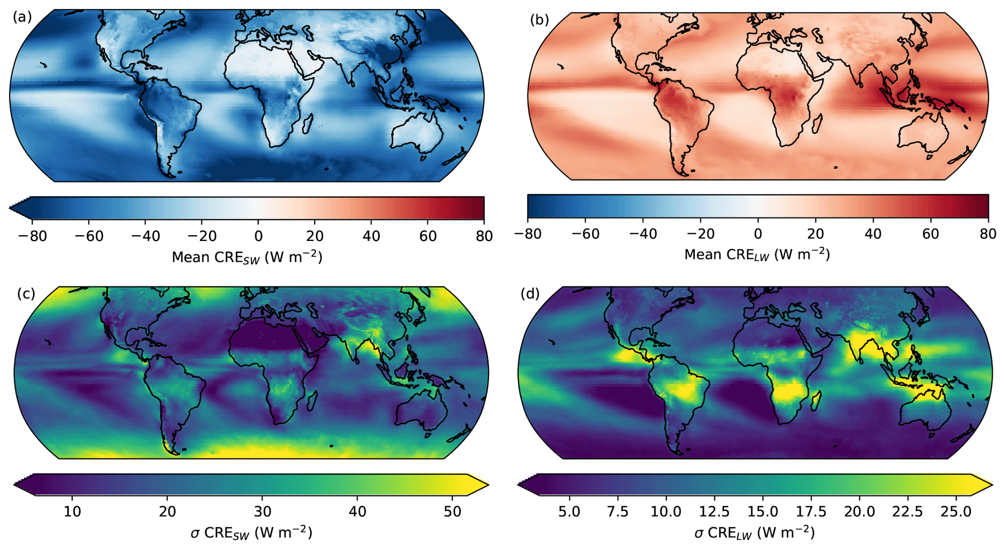
Figure 1 Climatological (2001–2020) mean (a, b) and standard deviation (c, d) of CRE_SW (a, c) and CRE_LW (b, d) from the CERES EBAF data. Pointy ends of the color bars indicate that the entire value range is not shown in the figure to improve its clarity.

Information on meteorological CCFs is taken from ERA5 (Hersbach et al., 2020), the newest reanalysis product from the European Center for Medium-Range Weather Forecasts (ECMWF). The following data are used from the surface layer of the reanalysis: sea surface temperature (SST), wind speed at 10 m (WS10), mean surface latent and sensible heat fluxes (MSLHF, MSSHF), and mean sea level pressure (MSL) (Wood, 2012; Fuchs et al., 2018; Scott et al., 2020). Data from pressure levels at 925, 700, 500, and 300 hPa are used for information on relative humidity (RH), air temperature (T), and the U, V, and vertical pressure velocity (ω) components of wind (Andersen et al., 2017; Fuchs et al., 2018; Ge et al., 2021; Grise and Kelleher, 2021; Kärcher, 2018; Kelleher and Grise, 2019; Patnaude et al., 2021). Data from pressure levels are referred to as X_zzz in this paper, where X is the abbreviation of the variable name, and _zzz is the pressure level (e.g., T₉₂₅ for air temperature at 925 hPa). In addition to these CCFs, information on estimated inversion strength (EIS; Wood and Bretherton, 2006) and horizontal temperature advection at the surface (T_adv; Scott et al., 2020) is derived from ERA5 reanalysis data. The set of CCFs therefore expands upon those traditionally used for cloud-regime-specific analyses (e.g., low clouds; see Scott et al., 2020) by including information on surface fluxes, vertically resolved proxies for dynamics (three-dimensional winds), and temperature and humidity profiles to account for mechanisms controlling different cloud types and altitudes. It is assumed that the observed cloud radiative effects are a response to the CCFs chosen, even though clouds can also feed back to contribute to CCF variability (e.g., Myers et al., 2018). All data are downloaded as monthly means at the native resolution of $\mathrm{0.25}{}^{\circ }\times \mathrm{0.25}{}^{\circ }$. T_adv is the exception to this rule, as using the monthly means of the U- and V-wind components at 10 m (U₁₀, V₁₀) would lead to an underestimation of the temperature advection (because U and V can be positive and negative and a temporal average is thus closer to 0). Due to this, T_adv is calculated from hourly U₁₀, V₁₀, and SST data at a spatial resolution of $\mathrm{2.5}{}^{\circ }\times \mathrm{2.5}{}^{\circ }$ (which corresponds to the length scale of 5^∘ as centered differencing is used for the calculation of the gradients) and then averaged to monthly means.

As satellite-retrieved aerosol proxies are not great proxies for CCN at cloud base (Stier, 2016) and feature the retrieval biases close to clouds discussed above, aerosol information from the MERRA-2 reanalysis is also used. The MERRA-2 aerosol reanalysis corrects the MODIS aerosol optical depth used for assimilation in the reanalysis for retrieval biases in humid environments and near clouds (Randles et al., 2017). From MERRA-2, sulfate aerosol concentrations (s) are used as in McCoy et al. (2017), McCoy et al. (2018), and Wall et al. (2022) by calculating monthly averages from the 3-hourly mean s at 910 hPa. The data are available at a spatial resolution of $\mathrm{0.5}{}^{\circ }\times \mathrm{0.626}{}^{\circ }$. As aerosol–cloud relationships tend to be linear at log scales, the base-10 logarithms of s, AOD, and AI are used in the statistical model (Wall et al., 2022).

2.2 Ridge regression

CRE_SW and CRE_LW anomalies are regressed on n (here: n=28) predictors so that each can be expressed as a linear combination of the local standardized CCF anomalies $X_i^{\prime }$:

$${\text{CRE}}^{\prime }=\sum _{i=\mathrm{1}}^n\left({\displaystyle \frac{\mathit{\delta }\text{CRE}}{\mathit{\delta }{X}_i}}\right)\times X_i^{\prime }+\text{Res},$$

with Res describing a catch-all mean-zero random error term. A major challenge when using a high number i of predictors X_i (in particular when considering a relatively small number of samples) to predict a target variable can be collinearity among predictors. In classical statistical techniques (e.g., OLS), collinearity frequently leads to high variance in the regression parameters (i.e., overfitting). Model variance can be reduced with regularization, which in the case of linear models is done by shrinking model coefficients towards zero by penalizing their size (Hastie et al., 2001). Ridge regression is a specific regularized linear model that has been shown to perform particularly well in the case of collinearity among the predictors (Dormann et al., 2013). Ridge regression makes use of the L2 penalty: the squared magnitude of the coefficient (β, here: $\frac{\mathit{\delta }\text{CRE}}{\mathit{\delta }{X}_i}$) value is added to the loss function, where the shrinkage is controlled by a value λ.

$${\text{Loss}}_{\mathrm{ridge}}=\text{Error}\left(Y-\widehat{Y}\right)+\mathit{\lambda }\sum _{\mathrm{1}}^n{\mathit{\beta }}_i^{\mathrm{2}}$$

Tuning the parameter λ involves a direct trade-off between a more flexible regression model (small penalty, i.e., low λ value) that may suffer from high-variance issues and a less flexible regression model (high penalty, high λ) that may have a larger bias. When λ is set to 0, the penalty is 0 as well so that the ridge regression is essentially an ordinary least-squares regression (James et al., 2021). A λ greater than 0 helps deal with collinearity by reducing model variance and in the case of many predictors thus provides more robust sensitivity estimates. Here, the optimal λ value is derived through leave-one-out cross-validation by probing 1000 evenly spaced λ values on a log scale between −3 and 5 in each $\mathrm{5}{}^{\circ }\times \mathrm{5}{}^{\circ }$ grid box. Leave-one-out cross-validation is the default cross-validation strategy for ridge regression, as it is extremely cost-efficient for least-squares regression (James et al., 2021) and has been found to reliably find the optimal level of regularization in the case of ridge regression (Patil et al., 2021). The λ values that lead to the best model performance in the cross-validation are shown in Fig. 2. To end up with a consistent regularization, the median λ value chosen in all cross-validations (median λ=12 for both CRE_SW and CRE_LW) is fixed. This means that the final regularized models are not optimized locally but that a representative λ value is chosen from the cross-validations to achieve comparable model coefficients across all regions. The differences between the predictive skill in the locally optimized and λ=12 settings have been found to be negligible, even in regions where optimal λ has been found to be >50. The data are split into a training (2001–2015) and a test (2016–2020) set. Cross-validation and training are done based on the training data, and the model performance is evaluated based on the test data. While the skill to predict CREs in the test is only marginally improved when using ridge regression instead of an ordinary least-squares regression (OLS), the OLS tends to fit very large, spatially noisy coefficients that are physically inconsistent (see Fig. A1).

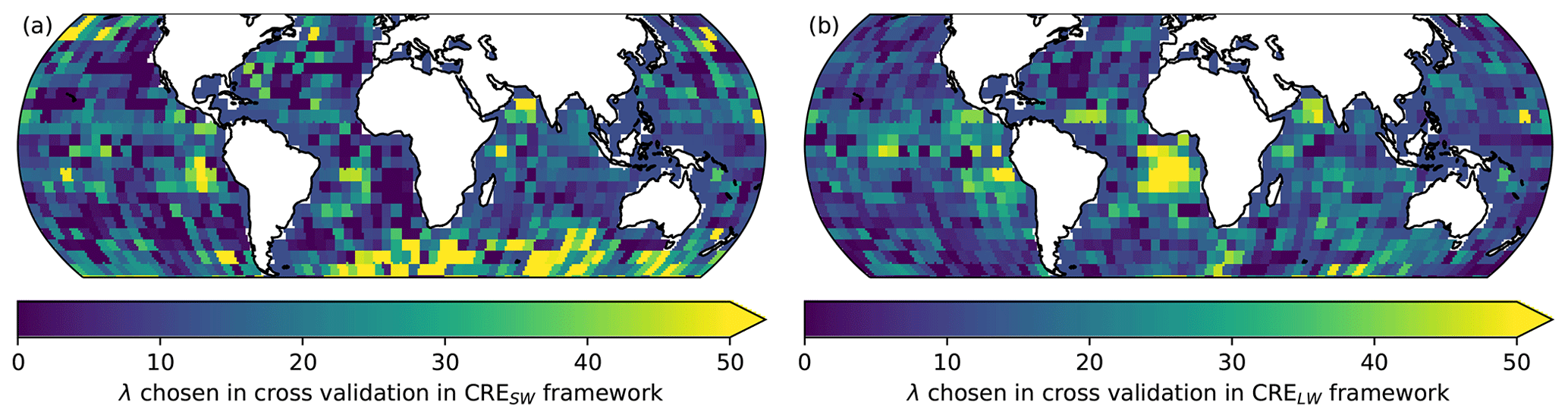
Figure 2 Spatial patterns of the λ chosen in the cross-validation at each grid box. The spatial median of λ is chosen as the regularization strength for each grid box in the final model training. To achieve comparable sensitivity estimates across different regions, the median λ value of 12 is chosen for the following analysis.

Three separate CCF frameworks are trained for CRE_SW and CRE_LW using a different aerosol parameter each time. The meteorological sensitivities presented in this study refer to those derived from the log ₁₀s setup. The regression coefficients of the ridge regression represent the sensitivity of CREs to a 1 standard deviation change in the local monthly anomalies in each CCF with all other local meteorological conditions held fixed and are thus given as W m⁻² σ⁻¹ (for sensitivity). As total CREs are used as a predictand (rather than specific cloud properties or CREs of a specific cloud type), the sensitivities are a top-down estimate of the total radiative response by all clouds to changes in CCFs within each grid box. In general, positive CRE_SW sensitivities mean that an increase in a CCF is connected to a reduction in the shortwave cooling effect of clouds from reflected solar radiation (e.g., by reducing cloud amount or reflectivity), whereas positive CRE_LW sensitivities relate the increase in a CCF to a stronger longwave warming effect of clouds (more clouds or higher and/or colder clouds that effectively trap more longwave (LW) radiation from surfaces below than they emit). As such, one can expect that CRE_SW and CRE_LW sensitivity patterns are generally anticorrelated. Sensitivities of radiative effects of undetected very thin clouds and the transition zone between aerosols and clouds obviously cannot be captured though (Eytan et al., 2020; Jahani et al., 2022).

2.3 Cloud regimes

While the regression models are trained to predict CREs with the same set of CCFs independently of the region (and thus dominant cloud regime) considered, climatological cloud regime regions are used to analyze the resulting sensitivities specifically for four regions: stratocumulus (Sc), trade cumulus (Tc), tropical ascending (Ta), and midlatitudes (Ml). This is done to summarize sensitivities in climate regimes with similar cloud types, which are expected to be driven by different mechanisms and related to different cloud feedbacks (e.g., low-cloud feedback mainly in Sc vs. high-cloud feedback in Ta). The cloud regimes are defined based on climatological (2001–2020) EIS and ω₇₀₀ thresholds similar to Scott et al. (2020), based on Medeiros and Stevens (2011). The thresholds are given in Table 1 and lead to the cloud regime regions shown in Fig. 3.

Table 1 Thresholds to determine the cloud regime regions shown in Fig. 3.

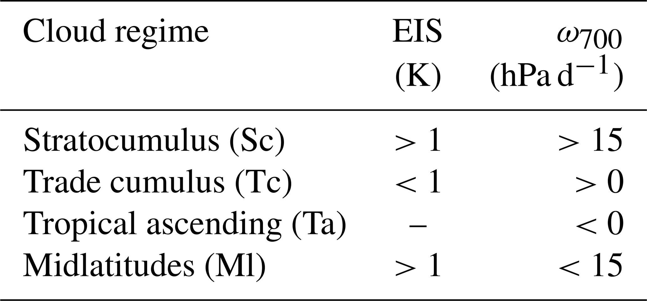
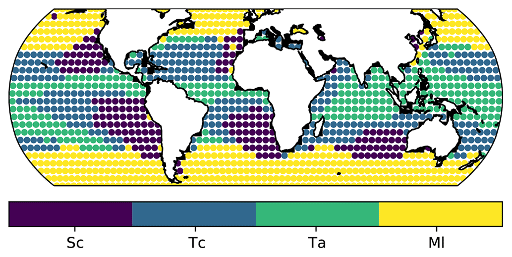
Figure 3 Cloud regimes derived from the EIS and ω₇₀₀ thresholds described in Table 1.

3 Results and discussion

3.1 Skill of the regression models

Figure 4 shows the skill of the ridge regression models to predict CRE_SW (left) and CRE_LW (right) in the independent test data (2016–2020). The models are able to capture about two-thirds of the temporal variability in CRE anomalies in the independent test data, with slightly better model performance for predicting CRE_LW than CRE_SW (global weighted average R² of 0.72 vs. 0.63, standard deviation of 0.13 and 0.21, respectively). The skill is thus markedly higher than the low-cloud frameworks from Scott et al. (2020) (0.37, or 0.51 when information on upper-level clouds is included) and Wall et al. (2022) (0.42). This shows that the added CCFs increase the predictive performance of the model, could indicate that they may help capture processes relevant to determine CREs, and may therefore allow for tighter constraints for cloud feedbacks and aerosol–cloud interactions than prior studies. The spatial pattern in the prediction skill of CRE_SW shows particularly good skill in the regions of the ascending tropical cloud regime (mean R²=0.81) and poorer performance in the midlatitudes (mean R²=0.40), especially over the Southern Ocean. The comparably poor skill in the Southern Ocean is notable, as numerical models also have large uncertainties and biases in modeling radiative fluxes and clouds here (Gjermundsen et al., 2021; McFarquhar et al., 2021). The poor model performance may be linked to the low quality of reanalysis data sets found in this region due to the limited number of measurements available for the assimilation (Mallet et al., 2023). A second possible reason for the low skill in this region may be that the CCFs may not adequately capture the influence of the large day-to-day variability of synoptic-scale dynamics on clouds of this region (Kelleher and Grise, 2019) at the monthly timescale. This is supported by findings from Jia et al. (2023), who use a machine learning framework to predict marine low cloud cover with a similar set of predictors at a daily timescale and achieve notably high skill over the Southern Ocean. In the Sc regime the average prediction skill of CRE_SW is 0.55, which seems to be markedly higher than in Scott et al. (2020) and Wall et al. (2022), even though the exact regime-specific skill is not reported in their studies. The skill in predicting CRE_LW is also highest in the tropics (mean R²=0.79) and trade cumulus regions (mean R²=0.77) and lower in the stratocumulus and Southern Ocean regions. This makes sense, as there is little CRE_LW variability in those regions due to the dominance of low clouds and hence only a small signal for the regression model to learn (see Fig. 1). Over the Southern Ocean, the assumed lower quality of the reanalysis data and the large influence of transient weather systems not being captured adequately at the monthly timescale may also contribute to the lower skill.

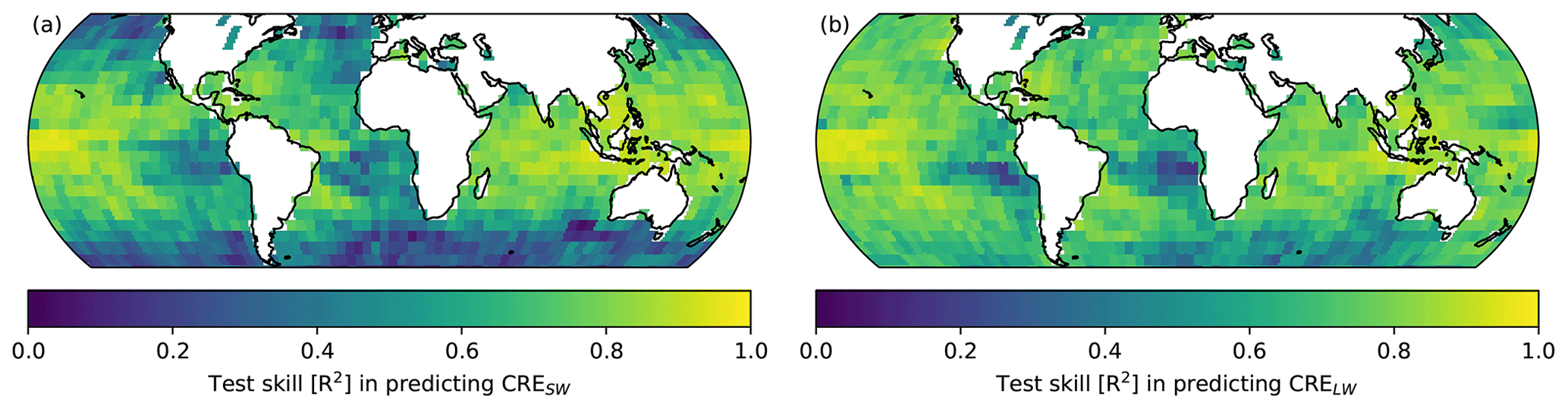
Figure 4 Skill (R² score) of the ridge regression models to predict CRE_SW (a) and CRE_LW (b) in the independent test data (2016–2020).

There is a significant (p value <0.01) negative correlation between the prediction skill of the ridge models (Fig. 4) and the regularization strength λ chosen in cross-validation (−0.34 for CRE_SW and −0.31 for CRE_LW). The regularization strength that optimizes model performance is higher in regions where model performance is comparatively low. This is an indication that in these regions where the predictors do not explain the CRE variability well, the regression coefficients are less certain, model variance is higher, and the increase in the model bias when the coefficients are nudged towards 0 (thereby predicting less CRE variability) is relatively small. Coefficients of selected CCFs estimated by the ridge regression are described in the following, with the focus on (1) SST and EIS as well-known low-cloud CCFs important for the low-cloud feedback, (2) three-dimensional winds at different pressure levels for information on large-scale dynamics that are often not part of CCF frameworks, and (3) aerosol proxies as a way of analyzing aerosol–cloud interactions in a CCF framework.

3.2 Sensitivity of CRE_SW and CRE_LW to SST and EIS

SST and EIS are the two main drivers of the marine low-cloud feedback (Myers and Norris, 2016; Myers et al., 2021; Klein et al., 2017; Cesana and Del Genio, 2021) and are thus discussed first. Figure 5 shows the spatial patterns of the sensitivity of CRE_SW (left) and CRE_LW (right) to SST (top) and EIS (bottom). The overall sensitivity of CREs to SST is dominated by the positive sensitivity of CRE_SW (global weighted mean 1.11 $\mathrm{W}{\mathrm{m}}^{-\mathrm{2}}{\mathit{\sigma }}^{-\mathrm{1}}$ compared to −0.12 $\mathrm{W}{\mathrm{m}}^{-\mathrm{2}}{\mathit{\sigma }}^{-\mathrm{1}}$ for CRE_LW). The CRE_SW sensitivity is particularly high in the stratocumulus regime (1.64 $\mathrm{W}{\mathrm{m}}^{-\mathrm{2}}{\mathit{\sigma }}^{-\mathrm{1}}$), which is to be expected, as these clouds are more strongly coupled to surface processes than, e.g., cumulus clouds in the trades (Wood, 2012; Cesana et al., 2019; Scott et al., 2020; Cesana and Del Genio, 2021). SST can influence low clouds via different mechanisms. Surface latent heat fluxes increase with SST, which enhances the buoyancy within the marine boundary layer and deepens it, leading to an increased entrainment of dry free-tropospheric air and thus evaporation of cloud water (Rieck et al., 2012; Qu et al., 2015). Also, increases in SST can lead to a stronger vertical moisture gradient, making dry-air entrainment more efficient in evaporating cloud (as the entrained air is relatively drier compared to the marine boundary layer air; Qu et al., 2015; van der Dussen et al., 2015), which has been shown to be the main cause of the recent decrease in low clouds off the coast of California (Andersen et al., 2022) where the SST–CRE_SW sensitivity is found to be largest. These findings generally agree with those of Scott et al. (2020), who specifically analyze low-cloud induced changes in radiative fluxes, although their average sensitivity estimate is lower and not positive in all regions, which may point to an underestimation of the positive low-cloud feedback found by Myers et al. (2021). CRE_LW sensitivities are in general negligible for the stratocumulus cloud regime, as their warm cloud tops only induce a minor CRE_LW. There is a systematic negative CRE_LW–SST sensitivity in the Tc regime (−0.29 $\mathrm{W}{\mathrm{m}}^{-\mathrm{2}}{\mathit{\sigma }}^{-\mathrm{1}}$), which is outweighed by the positive CRE_SW–SST sensitivity in that regime though (1.08 $\mathrm{W}{\mathrm{m}}^{-\mathrm{2}}{\mathit{\sigma }}^{-\mathrm{1}}$). Still, a negative CRE_LW–SST sensitivity in the Tc regime suggests that the overall (weak) low-cloud feedback in the Tc regime might be further reduced by the longwave effect partly balancing the shortwave effect. In the tropics, there is a band of moderate positive CRE_LW–SST sensitivity, indicative of more frequent or higher-reaching convection in cases of higher SSTs. As the CRE_SW sensitivity is only slightly negative in some of these regions, the results suggest that most of this positive CRE_LW sensitivity is driven by cloud altitude and temperature and not high cloud cover. While such local effects of SST on deep convection have been noted in the past (Zhang, 1993), non-local pattern effects of SST on deep convective CREs (Fueglistaler, 2019) cannot be captured with our approach.

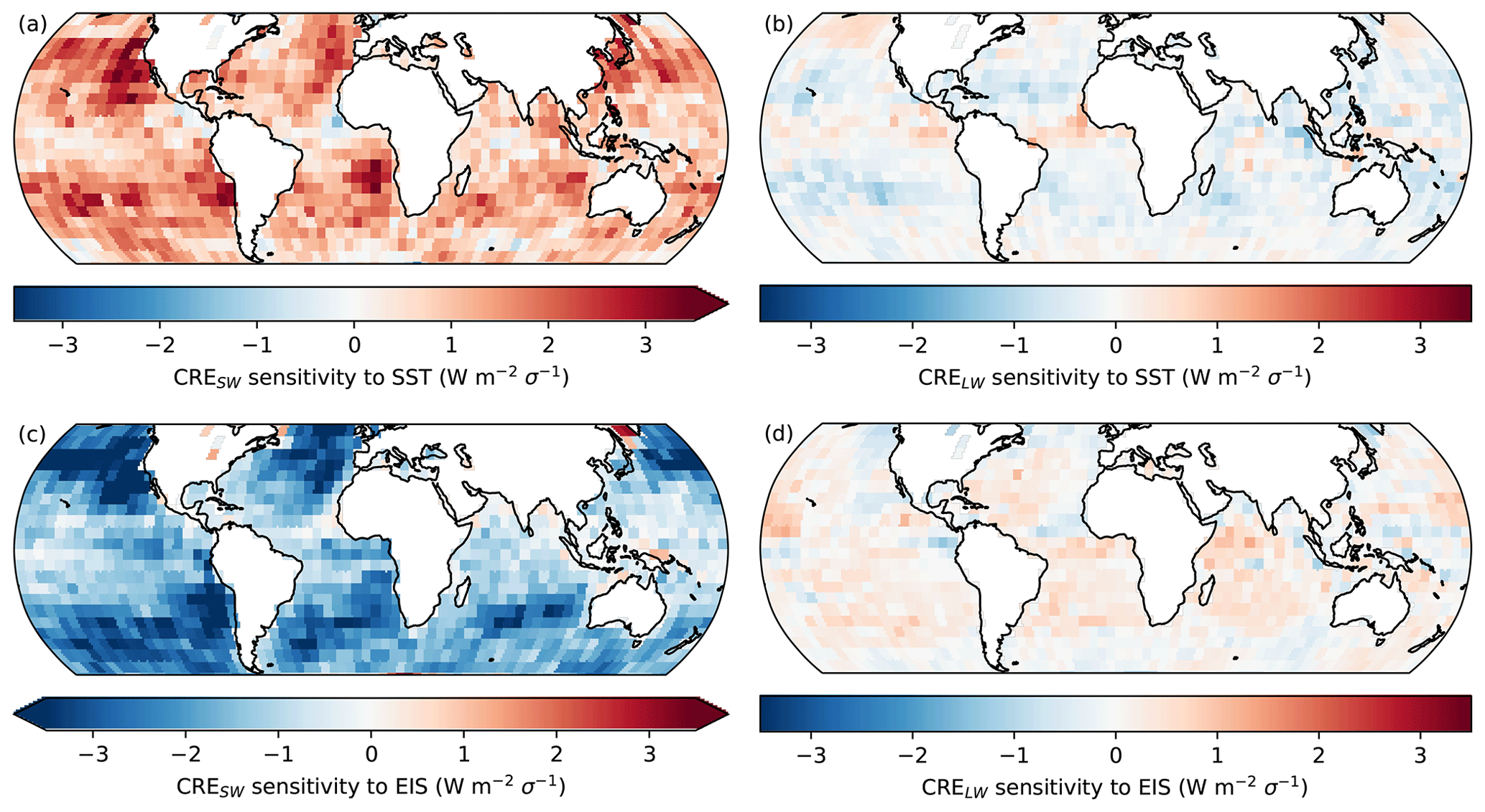
Figure 5 Sensitivity of CRE_SW (a, c) and CRE_LW (b, d) to SST (a, b) and EIS (c, d).

The sensitivity of CREs to EIS is dominated by the negative CRE_SW sensitivity (global weighted mean −1.57 $\mathrm{W}{\mathrm{m}}^{-\mathrm{2}}{\mathit{\sigma }}^{-\mathrm{1}}$), which is also particularly strong in the Sc regime (−2.33 $\mathrm{W}{\mathrm{m}}^{-\mathrm{2}}{\mathit{\sigma }}^{-\mathrm{1}}$) and the Ml (−1.97 $\mathrm{W}{\mathrm{m}}^{-\mathrm{2}}{\mathit{\sigma }}^{-\mathrm{1}}$) and smallest for the Ta regime (−0.91 $\mathrm{W}{\mathrm{m}}^{-\mathrm{2}}{\mathit{\sigma }}^{-\mathrm{1}}$). The results agree remarkably well with those found by Scott et al. (2020) in both overall magnitude and spatial as well as regime patterns. EIS modifies low clouds by controlling the amount of dry entrainment from the free troposphere into the marine boundary layer, where a strong inversion limits this entrainment and leads to a shallower marine boundary layer effectively trapping moisture. This has been observed particularly in the Sc and Southern Ocean regimes (Klein and Hartmann, 1993; Wood and Bretherton, 2006; Kelleher and Grise, 2019; Scott et al., 2020). There is only a limited, mainly positive sensitivity of CRE_LW to EIS, which is largest in the Tc regime (0.24 $\mathrm{W}{\mathrm{m}}^{-\mathrm{2}}{\mathit{\sigma }}^{-\mathrm{1}}$). This is due to the moderate LW warming exerted by an increase in Tc clouds. The overall low magnitude of the CRE_LW–sensitivity to EIS is expected, as, similar to SST, EIS mainly drives low-cloud variability.

3.3 Sensitivity of CRE_SW and CRE_LW to large-scale circulation

Variability in large-scale circulation and dynamics is mainly approximated by anomalies in the three-dimensional winds at different pressure levels (300, 500, 700, and 925 hPa). The sensitivity of CREs to variations in the vertical pressure velocity ω is largest at 300 hPa, which is the strongest predictor for CREs in general in the ascending tropics (Fig. 6). The sensitivity of CRE_SW and CRE_LW is nearly balanced for ω₃₀₀, but less so for ω₉₂₅, where ω within the boundary layer mostly influences low clouds and thus CRE_SW. In the free troposphere at 700 hPa, ω is only a minor control of CRE variability. The sensitivity patterns of CRE_SW and CRE_LW to ω₃₀₀ (Fig. 7) closely follow the regions of tropical ascent and reach maximum values in the tropical warm pool region. In the Ta regime, ω₃₀₀ anomalies are shown to lead to a strong cooling from the CRE_SW (2.51 $\mathrm{W}{\mathrm{m}}^{-\mathrm{2}}{\mathit{\sigma }}^{-\mathrm{1}}$) that is nearly completely balanced by a strong warming from the CRE_LW (−2.01 $\mathrm{W}{\mathrm{m}}^{-\mathrm{2}}{\mathit{\sigma }}^{-\mathrm{1}}$) by the increase in upper-level clouds. While the nearly exact opposite mirroring of the CRE sensitivity patterns to ω₃₀₀ (correlation coefficient −0.86 globally and −0.81 in the Ta regime) can partly be explained by the overall balance of CRE_SW and CRE_LW in this region (Fig. 1), it is noteworthy, since the cancellation of CRE_SW and CRE_LW is the result of a mixing of various cloud types with very specific CRE signatures (Hartmann and Berry, 2017; Wall et al., 2019). This seems to confirm that ω₃₀₀ is a strong predictor for the occurrence of most (deep) convective and cirrus clouds that dominate the CREs in the Ta regime (Ge et al., 2021).

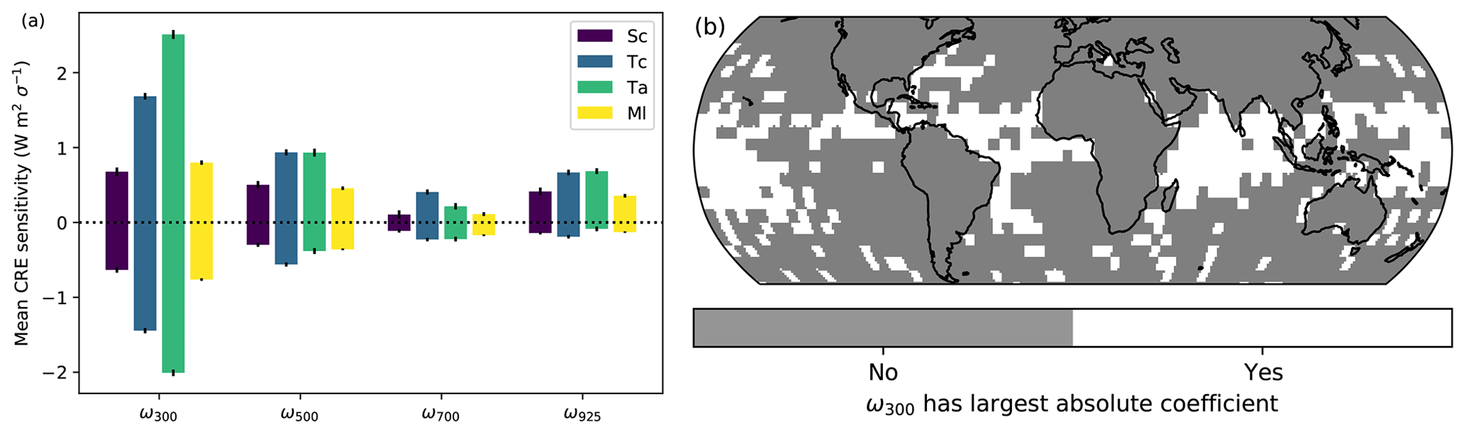
Figure 6 (a) Mean CRE sensitivity to ω at different pressure levels and for different cloud regime regions (denoted by the color). CRE sensitivities that are positive are always from CRE_SW, and negative ones are from CRE_LW. The error bars denote the standard error of the mean value ($\mathit{\sigma }/\sqrt{n}$), with n= being the sample size. (b) Map showing the regions where ω₃₀₀ has the largest absolute coefficient for CRE_SW.

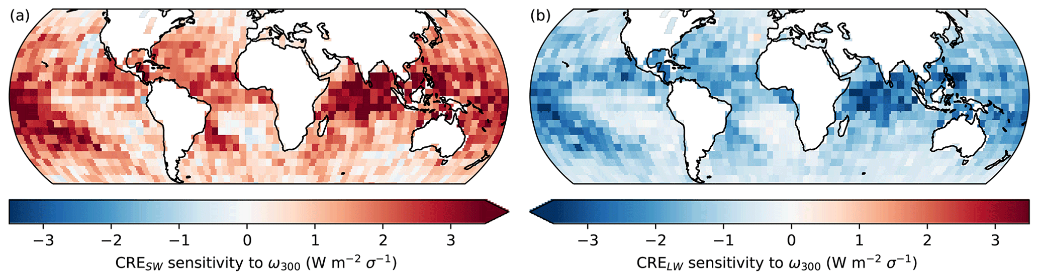
Figure 7 Sensitivity of CRE_SW (a) and CRE_LW (b) to ω₃₀₀.

CRE sensitivity to variability in zonal and meridional winds is most pronounced at 700 hPa and in the subtropics. The sensitivities to U₇₀₀ and V₇₀₀ anomalies (Fig. 8) are not trivial to understand, as they can be related to a change in wind speed or direction, dependent on the sign and climatological average of the wind component. In the following, these controlling factors are therefore explored in more detail.

Figure 8 Sensitivity of CRE_SW and CRE_LW to U₇₀₀ (a and b, respectively) and V₇₀₀ (c, d). Note the smaller sensitivity range in the color bar when compared to Figs. 5 and 7 (−2.5 to 2.5 vs. −3.5 to 3.5).

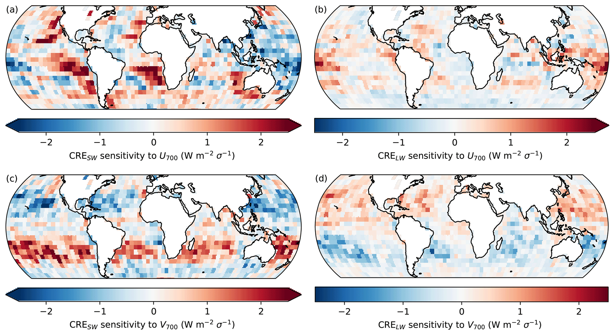
CRE_SW is markedly sensitive to U₇₀₀ in the core stratocumulus regions (mean Sc 1.05 $\mathrm{W}{\mathrm{m}}^{-\mathrm{2}}{\mathit{\sigma }}^{-\mathrm{1}}$), where clouds are typically below that level (Zuidema et al., 2009). As the stratocumulus clouds do not have a marked CRE_LW, this pattern only exists for the CRE_SW. In these regions, a positive U₇₀₀ CRE_SW sensitivity suggests a decrease in cloudiness with a westerly anomaly of the wind at 700 hPa. The opposite is the case over a trade wind cumulus region of the tropical Pacific, even though the sensitivity is less pronounced. In the following, a composite analysis is used to better understand what drives variability of local U₇₀₀ and how that may be related to CREs in an exemplary subtropical low-cloud region. Figure 9 shows the composite of anomalies in CCFs when U₇₀₀ anomalies in the southeastern Atlantic at 17.5^∘ S and 2.5^∘ E (black x) are >1σ. Figure 9a shows the observed CRE_SW anomalies in these situations, which feature a region of marked positive anomalies (less clouds) with an anomaly of 5.41 W m⁻² locally at 17.5^∘ S and 2.5^∘ E. The top center panel shows MSL anomalies which feature a high-pressure anomaly over the midlatitudinal Atlantic that strongly modifies the free-tropospheric winds (i.e., drives the U₇₀₀ anomaly). As the climatological mean boundary layer flow in the southeastern Atlantic is from a southeasterly direction, a northwesterly anomaly in the free-tropospheric flow tends to increase the vertical wind shear at the top of the boundary layer (U-wind shear between 700 and 925 hPa shown panel c of Fig. 9). In a stratocumulus-topped boundary layer an increased vertical wind shear is known to cause additional turbulence at the cloud top and lead to stronger entrainment of dry air into the cloudy marine boundary layer. Stronger dry-air entrainment would then dissolve the clouds from the top (Kopec et al., 2016; Zamora Zapata et al., 2021), possibly explaining the observed reduction in clouds in these situations. The boundary layer humidity (RH₉₂₅) is markedly increased in the composite along the southwestern African coastline (panel d), which would presumably lead to an increase in cloudiness (contrary to what is observed). While synoptically driven destabilization (reduced EIS) has also been reported to influence low-level clouds in this region (de Szoeke et al., 2016; Fuchs et al., 2017) and can be observed here (panel e), the anomaly is not spatially collocated with the CRE anomaly (bottom center) and is thus unlikely to explain it. Panel (f) shows the average ridge regression contributions of the most important CCFs to the predicted local CRE_SW anomaly of the composite analysis (multiplying the average standardized anomaly of the composite times the coefficients at the marked X location). Overall, the observed local CRE_SW anomaly of these situations of 5.41 W m⁻² can be reproduced fairly well by the ridge regression model, even though it is somewhat underestimated (3.85 W m⁻²). It is clear that in these situations, U₇₀₀ has the largest contribution (4.51 W m⁻²) to the predicted CRE_SW anomaly, which cannot be explained by the other CCFs. The observed humidification of the boundary layer in these situations only partly balances the strong contribution from U₇₀₀ (contribution of RH₉₂₅: −2.22 W m⁻²). While vertical wind shear was not originally considered to be a CCF in the model, at this location in the southeastern Atlantic, vertical wind shear and U₇₀₀ are strongly correlated (−0.90), which is also the case in all stratocumulus regions (average correlation for the Sc regime: −0.74), so in these regions, U₇₀₀ can be thought of as a proxy for vertical wind shear. Based on the results presented here, the wind-shear-induced turbulence at cloud top leading to entrainment and low-cloud dissipation is likely the main cause for the observed decrease in cooling from low clouds associated with the conditions of the composite analysis and for the observed sensitivity of CRE_SW to U₇₀₀ anomalies in the Sc regime. As such, vertical wind shear is recommended to be further explored in CCF analysis, especially for low-cloud frameworks.

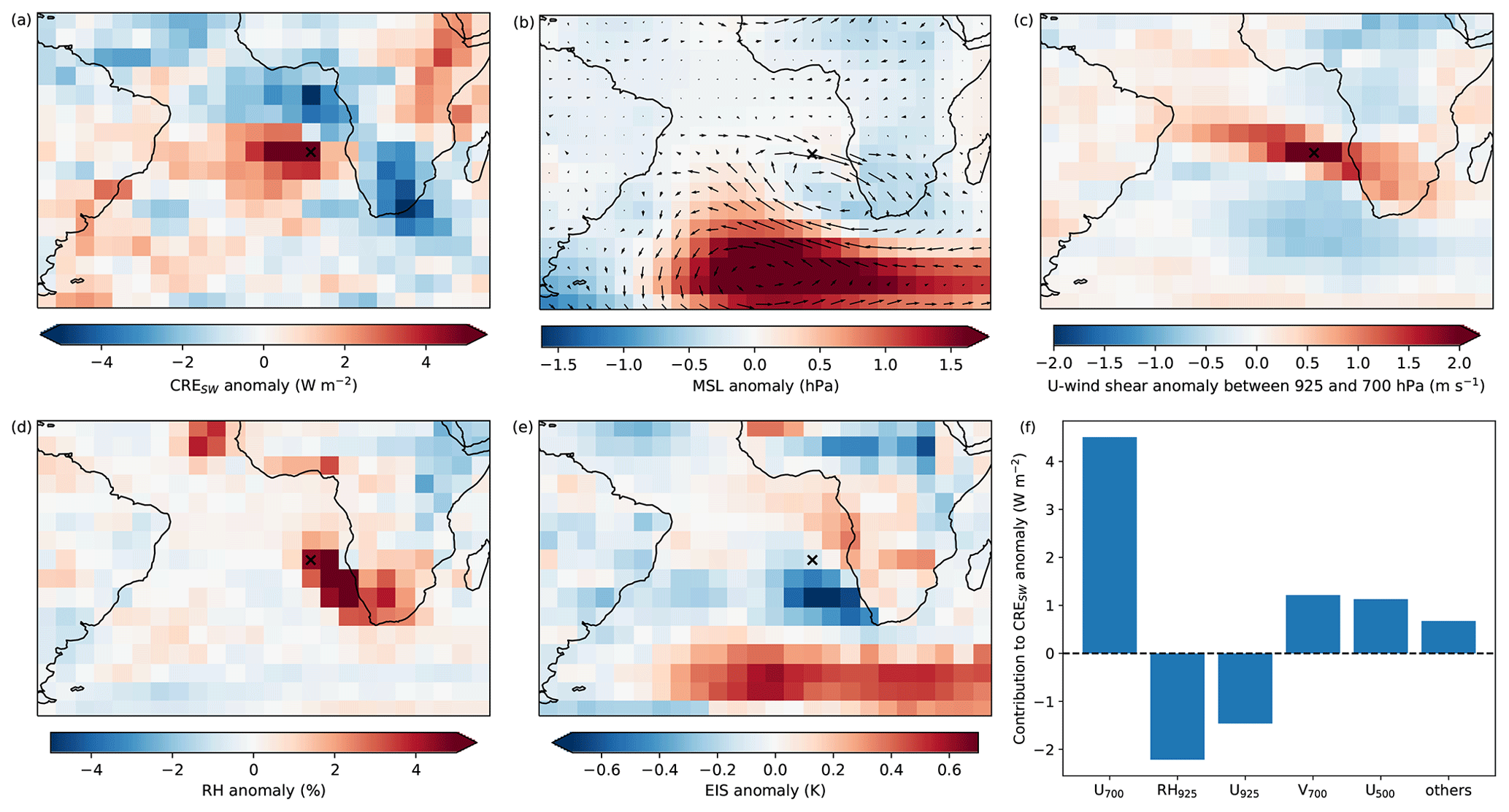
Figure 9 Composite analysis of anomalies in CCFs and CRE_SW when U₇₀₀ anomalies in the southeastern Atlantic at 17.5^∘ S and 2.5^∘ E (black x) >1σ. Panel (a) shows the observed CRE_SW anomalies in these situations. Panel (b) shows the MSL anomalies and wind anomalies at 700 hPa, and panel (c) shows the wind shear anomaly of the U component between the boundary layer (925 hPa) and the free troposphere (700 hPa). Panel (d) shows the RH anomaly in the boundary layer (925 hPa), and panel (e) shows EIS anomalies. Panel (f) shows the ridge-regression-quantified contributions of selected CCFs and the sum of all others to the predicted CRE_SW.

There is a coherent subtropical belt of a marked sensitivity of CREs to V₇₀₀ between ≈15 and 35^∘ with maximum sensitivity values between 20 and 25^∘ in each hemisphere (Fig. 8, bottom). The sensitivity has opposite signs depending on the hemisphere and the radiative effect considered and describes an increase in the cooling (CRE_SW) or warming (CRE_LW) effect of clouds connected to a poleward anomaly of the winds at 700 hPa. The zonal structure of the CRE_SW and CRE_LW sensitivities to V₇₀₀ is clearly visible in Fig. 10a. Figure 10b and c show a clear connection of poleward V₇₀₀ anomalies with large-scale ascent at the same pressure level and an increase in shortwave cooling from clouds (and vice versa). To give this finding more context, two composite analyses of situations with V₇₀₀>1σ in the South Atlantic and South Pacific regions are discussed in the following.

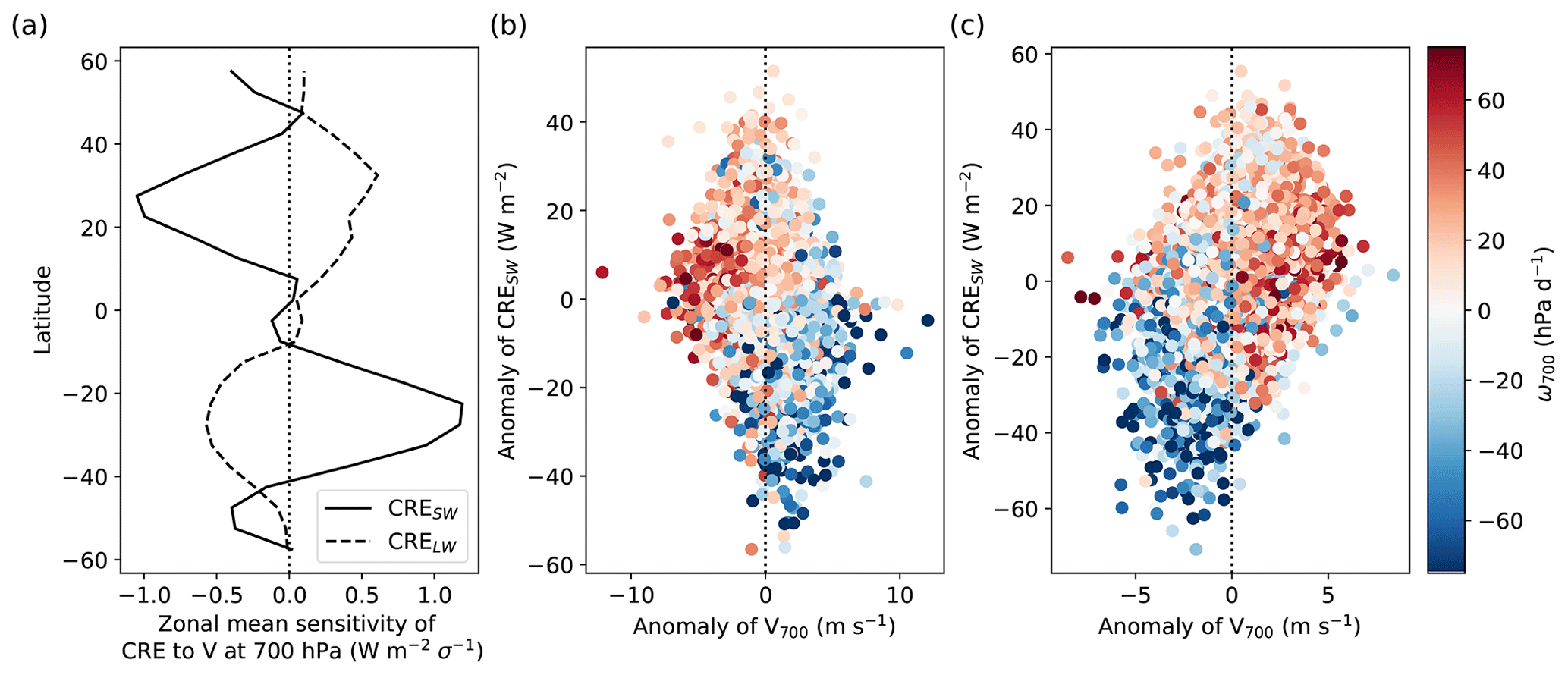
Figure 10 Summary of the CRE sensitivity to V₇₀₀ anomalies. (a) Zonal mean sensitivities of CRE_SW (solid line) and CRE_SW (dashed line) point to strong sensitivities in the subtropics. (b–c) The CRE_SW anomaly against the V₇₀₀ anomalies in the Northern (b) and Southern (c) Hemisphere where the absolute value of the sensitivity exceeds 1.5 $\mathrm{W}{\mathrm{m}}^{-\mathrm{2}}{\mathit{\sigma }}^{-\mathrm{1}}$, with the color showing ω₇₀₀ (blue: ascent, red: subsidence).

Figure 11 shows a connection of the conditions with V₇₀₀ anomalies >1σ to a subtropical low-pressure anomaly that is linked to a midlatitude synoptic-scale disturbance. The local poleward flow anomaly is clearly connected to a large-scale ascent anomaly which is causing an increase in humidity and clouds as well as a decrease in CRE_SW, confirming the observed correlations between V₇₀₀, ω₇₀₀, and CRE_SW presented in Fig. 10. While it is generally known that ascending air is the main mechanism by which air is saturated and clouds form, a positive association between low clouds and free-tropospheric ascent has also been found in subtropical regions of climatological subsidence (Myers and Norris, 2013). The results from this exemplary composite analysis are indicative of the poleward and upward vertical velocity phases of synoptic waves as well as midlatitude cyclones and the associated increase in cloudiness. The ridge regression can reproduce the local CRE_SW anomalies for these composites well (observed vs. predicted: Atlantic −7.37 W m⁻² vs. −6.36 W m⁻², Pacific −12.74 W m⁻² vs. −12.28 W m⁻²), and the quantified contributions to the predicted CRE_SW anomalies (bottom panels g and h) show that, indeed, the largest contributions come from ω and RH at different levels in the free troposphere and from V₇₀₀. There are two possible explanations for the CRE sensitivity to V₇₀₀: (1) the physical explanation is that the enhanced poleward winds on the eastern side of the midlatitude cyclones could be related to increased warm and moist advection, which increases cloudiness. (2) The statistical explanation is that V₇₀₀ anomalies are correlated with large-scale ascent, which is causing the clouds to form and additionally have a high signal-to-noise ratio for such midlatitude synoptic variability. By capturing this synoptic variability, V₇₀₀ anomalies would then encapsulate changes in a number of relevant CCFs (not only ω₇₀₀) related to the synoptic forcing and thereby be assigned the observed sensitivities. In this regard, it should be noted that an anomaly pattern similar to that of ω₇₀₀ can also be found for ω at 500 and 300 hPa, showing that the disturbance leads to vertically extended large-scale ascent. The question is to what degree the V₇₀₀ sensitivity and resultant contributions are the result of a physical connection between V₇₀₀ and CRE_SW in the subtropical belts or of the correlation of V₇₀₀ with ascending motion that is driving cloudiness. This question cannot directly be answered with this approach, highlighting the challenge of trying to untangle causality with statistical models and correlated inputs. The coherent association of V₇₀₀ anomalies and ω₇₀₀ (see Fig. 10) suggests that the composite analyses are likely representative for other regions in the subtropical V₇₀₀ sensitivity belt as well.

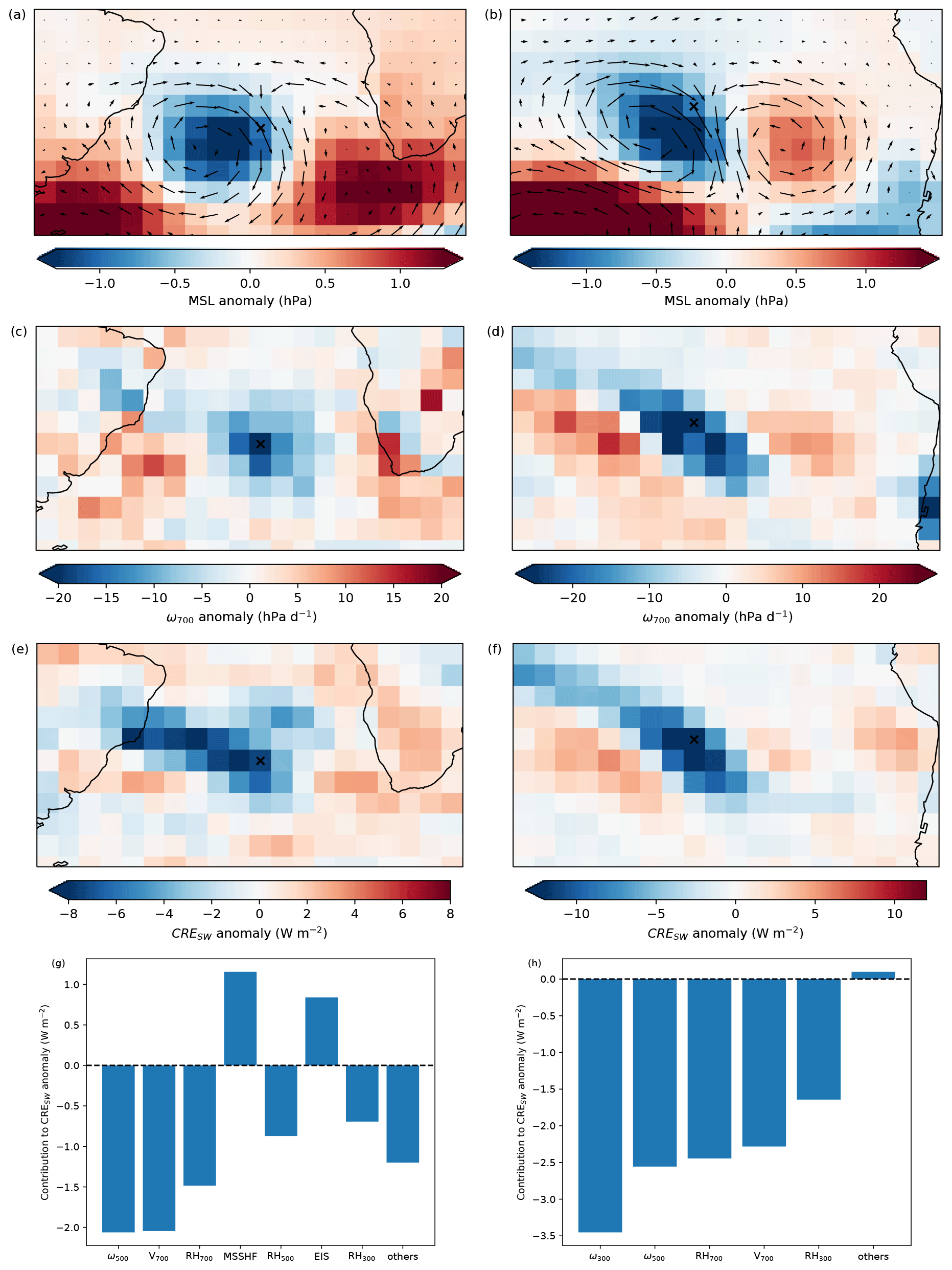
Figure 11 Composite analysis of anomalies in CCFs and CRE_SW when V₇₀₀ in the southeastern Atlantic (left: at 27.5^∘ S and 12.5^∘ W) and in the South Pacific (right: at 22.5^∘ S and 127.5^∘ W) >1σ. From top to bottom, the panels show MSL anomalies and wind anomalies at 700 hPa, ω₇₀₀ anomalies, observed CRE_SW anomalies, and ridge-regression-quantified contributions to the predicted CRE_SW anomaly.

3.4 Sensitivity patterns of CRE_SW and CRE_LW to aerosol proxies

CRE sensitivities to three different aerosol proxies (log ₁₀s, log ₁₀AI, and log ₁₀AOD) are described in the following. It should be noted that changing a CCF (here: the aerosol proxy) slightly changes other sensitivities as well. The magnitude of these changes depends on the aerosol proxies compared. Figure 12 shows the correlation of spatial sensitivity patterns among individual CCFs for different aerosol proxy combinations. It can be seen that when the two satellite-derived aerosol proxies are compared, all other sensitivity patterns stay nearly constant (average correlation 0.99 and 0.98 for CRE_SW and CRE_LW, respectively), and the derived spatial sensitivity patterns of log ₁₀AOD and log ₁₀AI are fairly strongly correlated as well. This is not surprising, as AOD and AI are directly related. In sensitivity estimates that use log ₁₀s as an aerosol proxy correlations amongst the other CCF sensitivity patterns are lower (on average ≈ 0.92–0.93), and the CRE log ₁₀s sensitivities are not strongly correlated with those of the satellite-derived aerosol proxies (0.21–0.31). When comparing the sensitivity patterns of the aerosol proxies in the following, the different nature of the aerosol data sets should be kept in mind: the satellite-derived AOD and AI are columnar retrievals, do not focus on a specific aerosol species, and suffer from retrieval biases close to clouds (especially the AOD), while the sulfate concentration from the aerosol reanalysis focuses on a single species at a level close to cloud base (for clouds forming in the marine boundary layer) and is expected to have reduced biases typical of satellite retrievals. However, the aerosol reanalysis may introduce different model-based biases, which are not well known. Findings from McCoy et al. (2017) indicate that the variable spatial emissions of diffuse natural sources of sulfate (e.g., marine biogenic dimethylsulfide) are not as well captured by MERRA-2 as emissions from anthropogenic source regions, leading to a spatial variability in the quality of the MERRA-2 sulfate data. While sulfate aerosols dominate the aerosol optical depth signal in many regions of anthropogenic emissions, continental outflow regions, and natural sources, they are not the main contributor in other regions (e.g., Southern Ocean; Li et al., 2022). In the regions where sulfate does not dominate CCN, log ₁₀s is not expected to be a good proxy for CCN at cloud base.

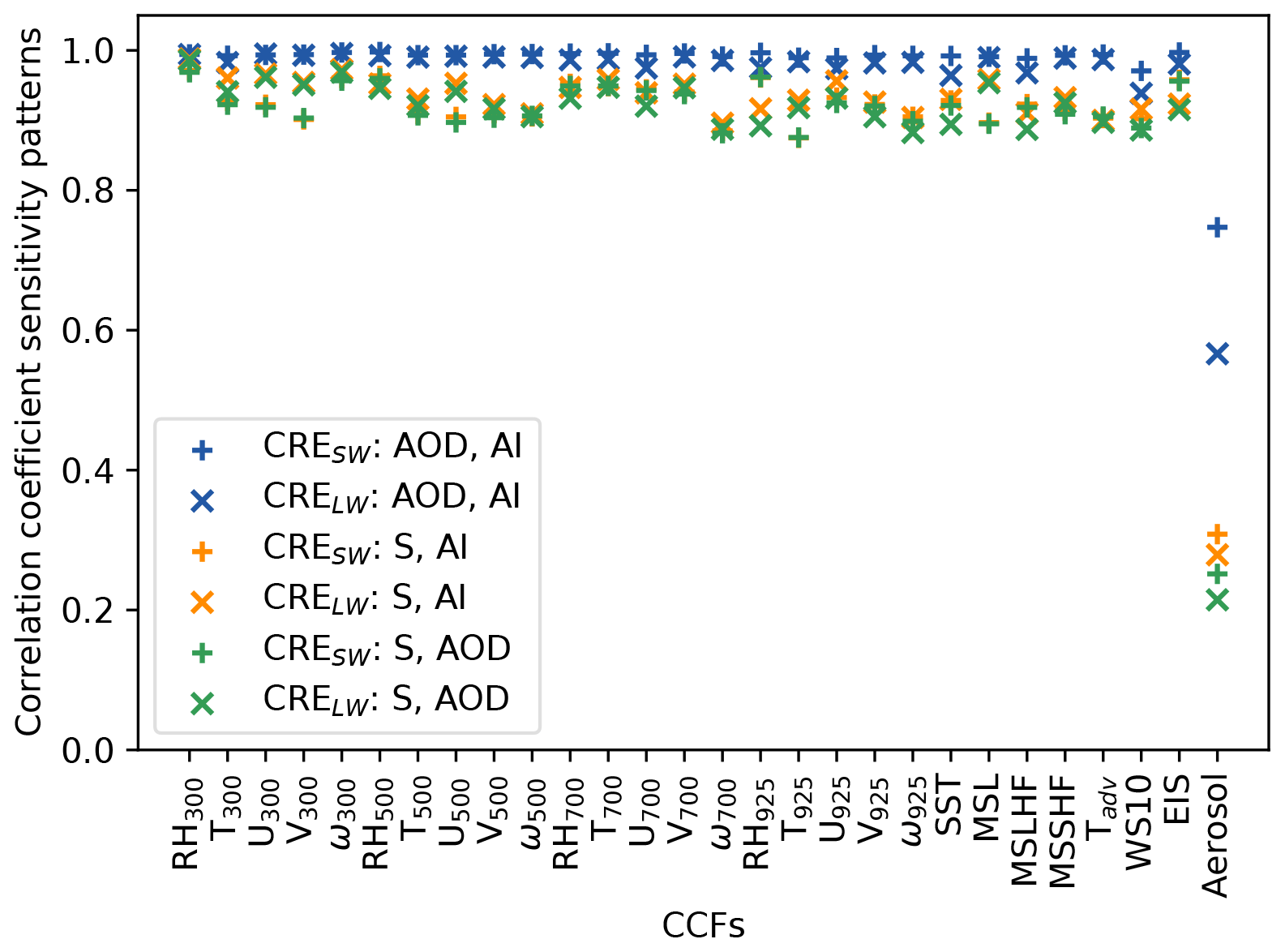
Figure 12 Correlation of spatial sensitivity patterns of all individual CCFs estimated by ridge regression models for different aerosol proxy pairs as noted in the legend. In this study only CRE sensitivities to meteorological CCFs from the log ₁₀s are shown.

The left-hand column of Fig. 13 shows CRE_SW sensitivity to the three aerosol proxies. It is apparent that all aerosol proxies feature a negative global weighted average sensitivity, with that of log ₁₀s being markedly smaller in magnitude (−0.17 $\mathrm{W}{\mathrm{m}}^{-\mathrm{2}}{\mathit{\sigma }}^{-\mathrm{1}}$) than those of log ₁₀AI (−0.25 $\mathrm{W}{\mathrm{m}}^{-\mathrm{2}}{\mathit{\sigma }}^{-\mathrm{1}}$) and log ₁₀AOD (−0.34 $\mathrm{W}{\mathrm{m}}^{-\mathrm{2}}{\mathit{\sigma }}^{-\mathrm{1}}$). Similar to the recent study by Wall et al. (2022), who explored the effects of log ₁₀s in a low-cloud-specific CCF framework, and other recent global studies (e.g., Hasekamp et al., 2019; Toll et al., 2019; Jia et al., 2021) sensitivities are strongest in the Sc regime with CRE_SW sensitivity to log ₁₀s of −0.43 $\mathrm{W}{\mathrm{m}}^{-\mathrm{2}}{\mathit{\sigma }}^{-\mathrm{1}}$, to log ₁₀AOD of −0.70 $\mathrm{W}{\mathrm{m}}^{-\mathrm{2}}{\mathit{\sigma }}^{-\mathrm{1}}$, and to log ₁₀AOD of −0.66 $\mathrm{W}{\mathrm{m}}^{-\mathrm{2}}{\mathit{\sigma }}^{-\mathrm{1}}$. A marked difference between the derived sensitivity patterns is that in the Ta regime: the CRE_SW sensitivity to log ₁₀s is negligible (−0.06 $\mathrm{W}{\mathrm{m}}^{-\mathrm{2}}{\mathit{\sigma }}^{-\mathrm{1}}$), whereas it is substantial for log ₁₀AI (−0.27 $\mathrm{W}{\mathrm{m}}^{-\mathrm{2}}{\mathit{\sigma }}^{-\mathrm{1}}$) and even larger for log ₁₀AOD (−0.50 $\mathrm{W}{\mathrm{m}}^{-\mathrm{2}}{\mathit{\sigma }}^{-\mathrm{1}}$). In general, the finding of a stronger sensitivity for the satellite-derived aerosol proxies is expected, in particular in the case of AOD, due to the retrieval issues discussed in Sect. 2.1. While the ridge regression does control for the large-scale meteorology, the sensitivity is still likely to be confounded for the satellite-derived aerosol proxies, as aerosol swelling can be expected to affect aerosol retrievals at much smaller scales. Another reason for the weaker sensitivity of CRE_SW to log ₁₀s in the Ta regime, especially the tropical Pacific, could be that in this region sulfate aerosols may not dominate the total CCN budget as sea salt particles also make a large contribution (Shinozuka et al., 2004) and that in such remote oceanic regions the diffuse natural sources of sulfate are unlikely to be perfectly represented in the aerosol reanalysis, potentially leading to spatially inaccurate emissions and concentrations (McCoy et al., 2017).

The right-hand column of Fig. 13 shows the sensitivity patterns of CRE_LW to the different aerosol proxies, with a positive global weighted mean sensitivity for all proxies (log ₁₀s: 0.05 $\mathrm{W}{\mathrm{m}}^{-\mathrm{2}}{\mathit{\sigma }}^{-\mathrm{1}}$, log ₁₀AI: 0.03 $\mathrm{W}{\mathrm{m}}^{-\mathrm{2}}{\mathit{\sigma }}^{-\mathrm{1}}$, and log ₁₀AOD: 0.44 $\mathrm{W}{\mathrm{m}}^{-\mathrm{2}}{\mathit{\sigma }}^{-\mathrm{1}}$). While the CRE_LW sensitivity is much smaller than the CRE_SW sensitivity for log ₁₀s and log ₁₀AI, this is not the case for log ₁₀AOD, especially in the Ta regime, where the sensitivity is large (0.87 $\mathrm{W}{\mathrm{m}}^{-\mathrm{2}}{\mathit{\sigma }}^{-\mathrm{1}}$). This is likely due to the (largely spurious) relationships between AOD and cloud fraction (Gryspeerdt et al., 2016; Andersen et al., 2017; Christensen et al., 2017) as well as cloud-top temperature (Gryspeerdt et al., 2014) that dominate the CRE_LW signal. It is notable that while log ₁₀AI produces a similar overall sensitivity pattern (correlation 0.57; see Fig. 12), the magnitude is lower by a factor of 17 in the Ta regime. Overall, CRE_LW sensitivity to aerosol proxies is large where the CRE_SW is large as well (correlations are −0.49 for log ₁₀s, −0.53 for log ₁₀AI, −0.69 for log ₁₀AOD), indicating that a large fraction of the quantified aerosol sensitivity is from the cloud adjustments that influence both CRE_SW and CRE_LW. In that sense it is expected that the correlation between the CRE_SW and CRE_LW sensitivity is particularly large for log ₁₀AOD, as it is particularly sensitive to aerosol swelling (thus spuriously relating AOD and cloud fraction). In the future, to better understand the differences in aerosol proxy–CRE relationships, a decomposition into cloud amount and radiative property changes in clouds may be helpful.

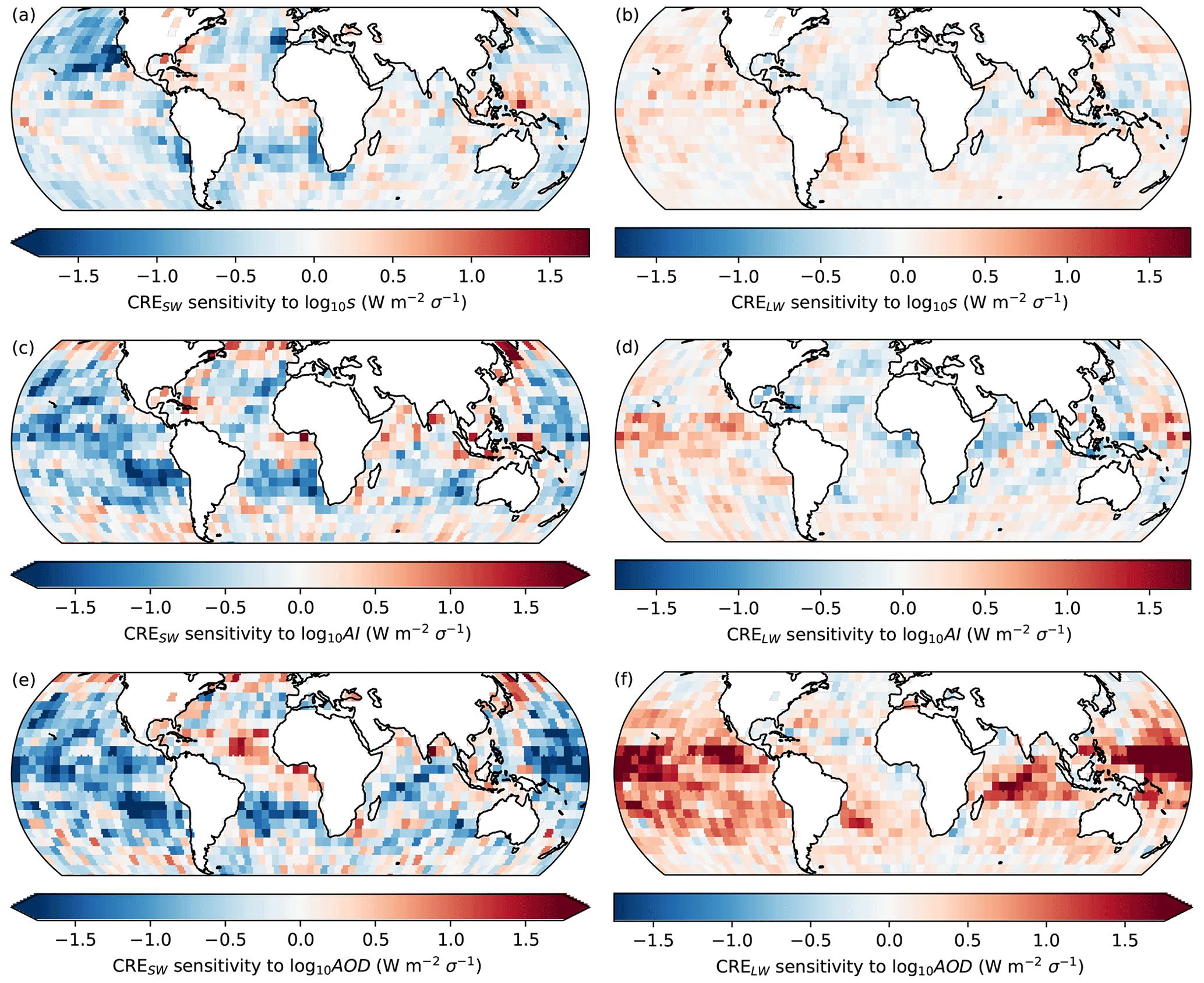
Figure 13 Sensitivity of CRE_SW (a, c, e) and CRE_LW (b, d, f) to log ₁₀s (a, b), log ₁₀AI (c, d), and log ₁₀AOD (e, f). Note that a smaller sensitivity range is shown compared to the other sensitivity maps.

4 Summary and conclusions

In this study, a regime-independent CCF framework was presented to predict near-global CRE_SW and CRE_LW. A regularized linear statistical learning technique (ridge regression) was used to quantify sensitivities of CRE_SW and CRE_LW to 28 CCFs, including three different aerosol proxies. The quantified sensitivities are investigated for selected CCFs and in regions of four broad cloud regimes. The most relevant findings are described in the following.

1. The statistical models are shown to be able to skillfully predict CRE_SW (global average R²=0.63) and CRE_LW (R²=0.72) in independent test data. Model skills are highest in the tropics and lower at high latitudes, in particular the Southern Ocean.

2. The sensitivity of CREs to the two most dominant low-cloud controls, SST and EIS, is most pronounced in the shortwave. It is strongest in regions where stratocumulus clouds dominate and largely consistent with other studies, suggesting an increase in low clouds with increasing EIS and decreasing SST. However, the sensitivity of CRE_SW to changes in SST is more spatially uniform than found in Scott et al. (2020), suggesting a possible underestimation of low-cloud feedback with planetary warming by Myers et al. (2021).

3. In the tropics, ω₃₀₀ is the most important CCF, influencing CRE_SW and CRE_LW in such a way that the effects of ω₃₀₀ nearly cancel out.

4. Zonal winds in the free troposphere are shown to be important proxies for synoptic variability relevant for subtropical CREs. U₇₀₀ anomalies are shown to be a good proxy for changes in vertical wind shear between the boundary layer and the free troposphere and thus the generation of turbulence at cloud top, leading to the depletion of low clouds. Vertical wind shear should thus be included and explored in CCF frameworks, in particular in low-cloud studies.

5. CRE is shown to be sensitive to V₇₀₀ in the subtropics, where poleward V₇₀₀ anomalies are linked to increased cooling from clouds. It is unclear, though, to what degree the V₇₀₀ sensitivity is related to warm, moist meridional advection that may increase cloudiness or may be driven by the correlation of V₇₀₀ with large-scale ascent in the region, which may lead to nonphysical statistical associations.

6. The CRE sensitivities to the three aerosol proxies (log ₁₀s, log ₁₀AI, and log ₁₀AOD) share the average sign (negative for CRE_SW and positive for CRE_LW) and have some qualitative similarities (CRE_SW sensitivity strongest in the stratocumulus regime). However, CREs are much more sensitive to log ₁₀AI and log ₁₀AOD in the tropics than to log ₁₀s. Differences between the sensitivities of CRE to the three aerosol proxies can be explained by retrieval biases (confounded relationships) and the varying contributions of log ₁₀s to CCN globally.

The statistical framework suggested here and the derived sensitivity patterns can be used in future cloud feedback analyses and to compare relationships between CCFs and CREs in global climate model output.

Appendix A

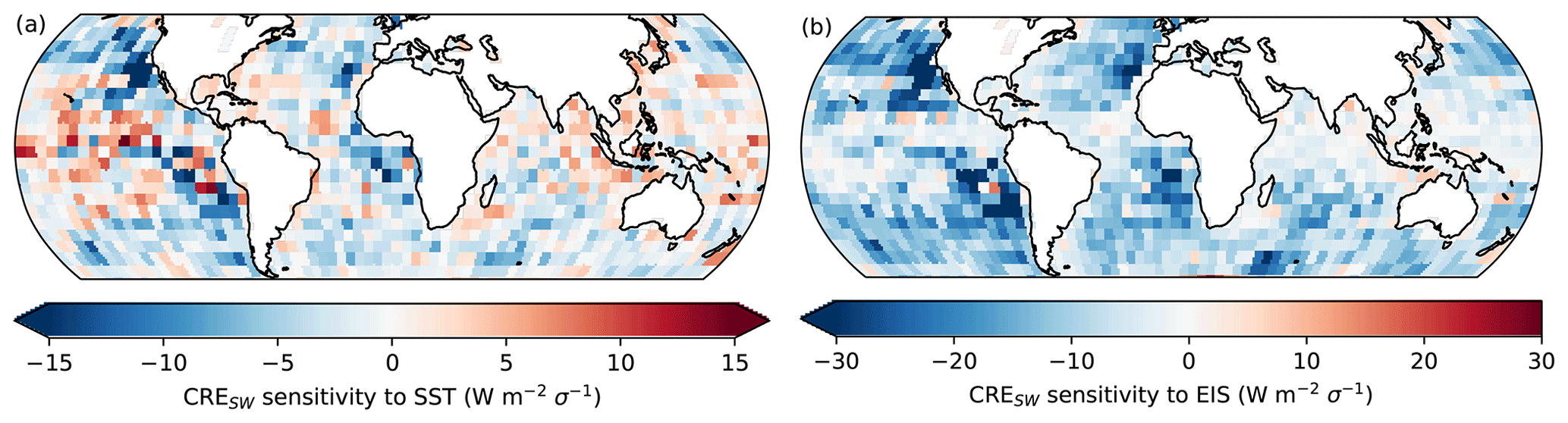
Figure A1 Sensitivity of CRE_SW to SST (a) and EIS (b) with λ set to 0 (OLS). The regression models are overfitting to the training data, resulting in much larger, noisy, and (in the case of SST) physically inconsistent sensitivity patterns.