Distinct regional meteorological influences on low-cloud albedo susceptibility over global marine stratocumulus regions

Marine stratocumuli cool the Earth effectively due to their high reflectance of incoming solar radiation and persistent occurrence. The susceptibility of cloud albedo to droplet number concentration perturbations depends strongly on large-scale meteorological conditions. Studies focused on the meteorological dependence of cloud adjustments often overlook the covariability among meteorological factors and their geographical and temporal variability. We use 8 years of satellite observations sorted by day and geographical location to show the global distribution of marine low-cloud albedo susceptibility. We find an overall cloud brightening potential for most marine warm clouds, which is more pronounced over subtropical coastal regions. A weak cloud darkening potential in the annual mean is evident over the remote SE Pacific and SE Atlantic. We show that large-scale meteorological fields from the ERA5 reanalysis data, including lower-tropospheric stability, free-tropospheric relative humidity, sea surface temperature, and boundary layer depth, have distinct covariabilities over each of the eastern subtropical ocean basins where marine stratocumuli prevail. This leads to a markedly different annual cycle in albedo susceptibility over each basin. Moreover, we find that basin-specific regional relationships between key meteorological factors and albedo susceptibilities are absent in a global analysis. Our results stress the importance of considering the geographical distinctiveness of temporal meteorological covariability when scaling up the local-to-global response of cloud albedo to aerosol perturbations.

1 Introduction

Marine warm (liquid) clouds cover about one-third of the global ocean surface in annual mean (Chen et al., 2014). They prevail over low-latitude to mid-latitude oceans and more pronouncedly over the eastern subtropical oceans where the Earth's major semi-permanent marine stratocumulus decks form (Klein and Hartmann, 1993; Wood, 2012). These bright and blanket-like stratiform clouds reflect a good fraction of the incident solar radiation (ranging from 0.35 to 0.42 in annual mean; Bender et al., 2011) that would otherwise (in the absence of these clouds) be largely absorbed by the dark ocean (∼ 94 %), effectively cooling the Earth (e.g., Stephens et al., 2012). For warm clouds exhibiting constant macrophysical properties (e.g., liquid water path (LWP) and cloud cover), their brightness or cloud albedo (A_c), quantified as the ratio of the reflected shortwave flux to the incoming solar radiation at the top of atmosphere, is particularly sensitive to the droplet concentration (N_d) such that higher N_d accompanied by smaller drops makes the cloud more reflective (cloud brightening; Twomey, 1974, 1977). However, cloud macrophysical properties do change with time as the cloud system evolves, through precipitation, evaporation, and/or entrainment mixing processes (Wood, 2012). Microphysical changes in N_d and droplet sizes induced by aerosol perturbations can substantially modulate the rate and efficiency of these processes and thereby cause further adjustments in macrophysical properties and cloud albedo (e.g., Boucher et al., 2013; Ackerman et al., 2004; Bretherton et al., 2007; Jiang et al., 2006).

In nature, the responses of cloud macrophysical properties to N_d perturbations are always complicated by the variability driven by local meteorology, and for decades, the stated challenge and focus have been to untangle aerosol effects from covarying meteorological conditions (Stevens and Feingold, 2009). Simulations of marine boundary layer (MBL) clouds, in which meteorology can be easily controlled, indicate a bidirectional LWP adjustment to increasing N_d. For precipitating clouds, an increase in N_d induces smaller droplets that suppress condensate removal, eventually leading to an increase in LWP (brighter clouds; Albrecht, 1989). In the case of non-precipitating clouds, the reduced droplet sizes lead to weaker sedimentation fluxes at cloud tops (Bretherton et al., 2007) and faster evaporation (Wang et al., 2003; Xue and Feingold, 2006), which both cause stronger entrainment mixing that reduces cloud LWP, resulting in less reflective clouds.

Observations of cloud adjustments following anthropogenic aerosol perturbations confirm the bidirectional LWP responses (e.g., Chen et al., 2012; Trofimov et al., 2020), while the aggregated response remains uncertain (Malavelle et al., 2017; Toll et al., 2019; Christensen et al., 2022). This means that cloud LWP responses to increased N_d can either enhance or offset the microphysical brightening depending on the meteorological conditions. Progress has been made over the years towards establishing fundamental knowledge of the environmental state and regime dependence of cloud adjustments to aerosol perturbations. For inversion-capped MBL clouds, the budget of cloud condensate is regulated mainly by entrainment drying at cloud tops and the fraction of precipitation that reaches the surface, which are strongly dependent on the humidity in the free troposphere and the lower-tropospheric stability (Ackerman et al., 2004; Chen et al., 2014; Gryspeerdt et al., 2019). In part related to the atmospheric stability, clouds exhibit a much more negative LWP response to increased N_d in deep MBLs than those that reside in shallower MBLs (e.g., Possner et al., 2020; Toll et al., 2019). Furthermore, Dagan et al. (2015) show that the direction in which the cloud condensate responds to an increase in aerosol depends on an optimal aerosol concentration which is determined by thermodynamic conditions (temperature and humidity). Wood (2007) shows that cloud-base height is the key determinant of whether cloud thickness changes will enhance or offset the Twomey brightening.

Clearly, the spatiotemporally scaling up (e.g., local-to-global and/or transient-to-climatology) of cloud albedo responses to aerosol perturbations depends crucially on the frequency of occurrence of the environmental states that characterize cloud adjustments. However, the spatiotemporal distribution of the covariability between meteorological and aerosol conditions is understudied and often ignored in “untangling” studies. Mülmenstädt and Feingold (2018) state the need for a shift in attention from untangling aerosol effects from covarying meteorology towards embracing and understanding the covariabilities between them. The focus of this study is exactly on this point.

Using 8 years of satellite observations and the ERA5 reanalysis dataset (introduced in Sect. 2), we characterize the geographical distribution of marine warm cloud albedo susceptibility over global oceans from 60^∘ S to 60^∘ N (Sect. 3). We show that similar free-tropospheric and boundary layer conditions lead to different albedo susceptibilities in different stratocumulus basins (Sect. 4), attributed to the distinct temporal covariabilities among large-scale meteorological conditions (Sect. 5.1). We find distinct monthly evolutions of albedo susceptibility in different stratocumulus basins, covarying with each basin's low-cloud frequency of occurrence and aerosol conditions (Sect. 5.2). We conclude that a frequency-weighted global aggregation of albedo-susceptibility–meteorology relationships obscures regionally distinct features and thus provides a biased view on the environmental dependence of albedo susceptibility.

2 Data and methods

We obtain coincident marine low-cloud properties, including cloud optical depth (τ), cloud-top effective radius (r_e), low-cloud fraction (f_c), cloud LWP, cloud-top height (CTH), and top-of-atmosphere (TOA) shortwave (SW) fluxes from the Moderate Resolution Imaging Spectroradiometer (MODIS) (Platnick et al., 2003) and the Clouds and the Earth's Radiant Energy Systems (CERES; Wielicki et al., 1996) sensors on board the Terra and Aqua satellites (overpass ∼ 10:30 and ∼ 13:30 local time, respectively), which are integrated into the CERES Single Scanner Footprint (SSF) product edition 4 (level 2) with a footprint resolution of 20 km (Su et al., 2015). N_d is calculated following Zhang et al. (2022) for all CERES footprints with cloud effective temperature greater than 273 K, CTH less than 3 km, τ>3, r_e>3 µm, solar zenith angle $<\mathrm{65}{}^{\circ }$, and f_c>0.8 in order to minimize retrieval biases (Grosvenor et al., 2018; Painemal et al., 2013; Grosvenor and Wood, 2014). Footprint cloud properties are aggregated to 1^∘ spatial resolution, using only the above-mentioned cloudy footprints where N_d is retrieved, to match susceptibilities calculated for individual 1^∘ × 1^∘ satellite snapshots. At this scale, the confounding effect of meteorology on footprint (i.e., sub-1^∘) cloud properties is negligible (Goren and Rosenfeld, 2012, 2014). Therefore, linear least-squares log–log regressions of footprint properties are used to calculate albedo susceptibility $S_{\mathrm{0}}=\mathrm{d}\ln \left(A_{\mathrm{c}}\right)/\mathrm{d}\ln \left(N_{\mathrm{d}}\right)$ and radiative susceptibility $F_{\mathrm{0}}=\mathrm{d}\left(A_{\mathrm{c}}\right)/\mathrm{d}\ln \left(N_{\mathrm{d}}\right)\times f_{\mathrm{c}}\times {\mathrm{SW}}_{\mathrm{dn}}$; for both metrics, positive values indicate more reflected sunlight and thereby cooling, following Zhang et al. (2022). Note that since we are interested in the overall response of A_c to N_d perturbations, including both micro- and macro-physical adjustments, we do not stratify by LWP when calculating S₀. The result is that we obtain susceptibilities that account for both the Twomey effect and adjustments of cloud LWP. This differentiates our method from that of Painemal (2018) and Rosenfeld et al. (2019). Moreover, calculating S₀ from individual satellite snapshots enables us to associate the derived S₀ to the mean meteorological and cloud states of individual cloud scenes at a given space and time. The logarithmic transformation alleviates the dependence of S₀ on the absolute value of N_d, minimizing the impact of the remaining N_d retrieval biases (e.g., due to the adiabatic assumption). We do, however, use absolute values of A_c in the F₀ expression to obtain flux responses in units of watts per square meter (W m⁻²) instead of percentage responses.

Meteorological conditions, including sea surface temperature (SST), lower-tropospheric temperature, humidity, and wind profiles, are obtained from the European Centre for Medium-Range Weather Forecasts (ECMWF) fifth-generation atmospheric reanalysis (ERA5; Hersbach et al., 2020) and are interpolated and aggregated to the Terra and Aqua overpass times at 1^∘ spatial resolution. Lower-tropospheric stability (LTS) is calculated as the difference in potential temperature between 700 and 1000 hPa. Free-tropospheric relative humidity (RH_ft) is defined as the mean relative humidity between inversion top (defined as the level of the strongest gradient in temperature and humidity) and 700 hPa, following Eastman and Wood (2018).

The datasets span 60^∘ S to 60^∘ N, covering global oceans, from 2005 to 2012 (8 years). We screen for cloudy satellite scenes over open water when only single-layer liquid cloud (SLLC) is present. Aqua and Terra observations are analyzed separately, instead of collectively, in order to assess the robustness of our findings (qualitatively) and to explore the role of the diurnal cycle (quantitatively). Analyses using the Aqua observations are shown in the main text, and those using the Terra observations are shown in the Supplement, given the similarity between Aqua and Terra results. Regional annual maxima in SLLC fractional coverage and frequency of occurrence are used to identify five major marine stratus/stratocumulus regions (20^∘ × 20^∘; Fig. S1 in the Supplement, magenta boxes).

3 Global distribution of marine low-cloud albedo susceptibility

3.1 Annual mean

The climatology of the geographical distribution of marine low-cloud S₀ (Fig. 1a) is represented by an aggregation of susceptibilities derived from individual satellite snapshots over the 8-year period, taking into account the frequency of occurrence of different cloudy scenes and meteorological regimes. It is clear that over most parts of the global ocean (60^∘ S to 60^∘ N), low clouds have a positive S₀ (brightening) in the annual mean, which is more pronouncedly off the coast of continental land masses, although N_d is climatologically higher (Fig. S2) and the MBL is shallower (Fig. S3) compared to those over remote oceans. Only over the remote subtropical SE Pacific and SE Atlantic regions do the data show weak darkening potential (negative S₀) in the annual mean. The darkening potential means that the brightening of the clouds via the Twomey effect – i.e., more particles lead to more droplets and brighter clouds – is more than compensated for by liquid water losses.

Figure 1 Geographical distribution of marine single-layer low-cloud (a) albedo susceptibility (S₀) and (b) radiative susceptibility (F₀) weighted by the frequency of occurrence of single-layer liquid cloud (SLLC). Spatial-temporal averages of 5^∘ × 5^∘ areas are shown. Only areas with an SLLC frequency of occurrence greater than 0.1 are shown in (a). Magenta boxes in (a) indicate five 20^∘ × 20^∘ marine stratocumulus regions analyzed further in this study.

One can then translate the S₀ map into an annual flux perturbation potential map (Fig. 1b), which highlights the high annual cooling potential over subtropical stratocumulus regions even more by taking into account the cloud fraction and frequency and amount of incoming solar radiation at a given geographical location. In the remote parts of the subtropical stratocumulus decks, warmer SSTs deepen the MBL and encourage the entrainment of subsiding free-tropospheric air at cloud tops (Fig. S3; Bretherton, 1992; Wyant et al., 1997), favoring entrainment-feedback-driven LWP decreases with increasing N_d (Bretherton et al., 2007; Wang et al., 2003). The location where this MBL condition prevails is consistent with the location where we observe cloud darkening potential offsetting the Twomey brightening potential in the annual mean, resulting in a net warming potential over the SE Pacific and SE Atlantic (Fig. 1b).

3.2 Brightening versus darkening regimes

The LWP–N_d variable space has been shown as a useful framework to infer process-level understanding of aerosol–cloud interactions, using satellite observations (e.g., Zhang et al., 2022) or cloud-resolving simulation outputs (e.g Glassmeier et al., 2019; Hoffmann et al., 2020). Here we show S₀ in the LWP–N_d variable space for the five major stratocumulus regions (Fig. 2), similar to Fig. 3 in Zhang et al. (2022), where three clearly separated susceptibility regimes are evident. Note that, although S₀ is shown for each LWP–N_d bin, the calculation of S₀ applied to individual Terra/Aqua snapshots is not stratified by LWP (see details in Sect. 2), and thereby, both LWP adjustments (shown in Fig. S4) and the Twomey effect contribute to these albedo susceptibilities at different LWP–N_d states. The three regimes are as follows.

1. Precipitating–brightening. This regime consists of clouds with larger droplets (i.e., high cloud liquid water but low droplet number, i.e., to the left of the 12 µm isolines) that are likely to precipitate (Gerber, 1996; vanZanten et al., 2005). A positive susceptibility (brighter clouds with higher N_d) is consistent with the Twomey effect (microphysical adjustment; Twomey, 1974, 1977) and the precipitation-suppression-induced lifetime effect (macrophysical adjustment; Albrecht, 1989). Both effects contribute to the cloud brightening potential of this regime, and we do not attempt to separate them, as “untangling” is not the goal of this study. The focus on high-f_c scenes removes scenes with heavy precipitation, which is desirable since precipitation represents a cloud and/or rain effect on aerosol rather than an aerosol effect on cloud albedo.

2. Darkening. For clouds that are not heavily precipitating, cloud-top entrainment drives a negative tendency in cloud LWP that can overcome the positive tendencies driven by longwave (LW) cooling and surface fluxes and lead to cloud thinning and/or breakup (Hoffmann et al., 2020). A decrease in r_e and increase in N_d (assuming constant LWP when clouds respond microphysically to aerosol perturbations) lead to an increase in the overall droplet surface area, enhancing droplet evaporation; meanwhile, sedimentation fluxes at cloud tops reduce with smaller droplets. Enhanced evaporation and reduced sedimentation at cloud tops cause stronger entrainment mixing which further enhances evaporation and reduces sedimentation, creating positive feedback loops, termed the entrainment–evaporation feedback (EEF; Wang et al., 2003; Xue and Feingold, 2006) and the sedimentation–entrainment feedback (SEF; Bretherton et al., 2007), respectively. Moreover, SW heating during daytime, which can also be enhanced by increasing N_d and decreasing r_e, contributes to cloud thinning and/or breakup as well (Petters et al., 2012). Cloud states showing both negative LWP adjustment (Fig. S4) and negative S₀ (darker clouds with higher N_d) are evident in four of the five stratocumulus regions for thicker clouds (LWP >50 g m⁻²) with a higher droplet number concentration (N_d>50 cm⁻³) (Fig. 2b–d, f). This indicates that the Twomey effect is more than compensated for by these cloud-thinning processes that can be enhanced by a reduction in droplet sizes. Here we exclude the possibility of aerosol direct and semi-direct effects driving the cloud darkening, as the S₀ shown in this study is calculated at 1^∘ resolution, a scale at which we expect overlying absorbing aerosols to be spatially homogeneous.

3. Non-precipitating–brightening. For thinner non-precipitating clouds (LWP <50 g m⁻²), cloud-top entrainment efficiency is much reduced compared to thicker clouds (Hoffmann et al., 2020), and LW cooling surpasses SW heating at cloud tops (Petters et al., 2012), making it easy for the Twomey effect to overcome the cloud-thinning processes and dominate the A_c response. Moreover, weak positive correlations between LWP and N_d are observed for these non-precipitating thin clouds (Fig. S4). Although this contributes to the overall brightening potential, it does not necessarily represent an LWP adjustment to N_d changes. In fact, LWP may be the driver of this relationship when entrainment processes take a minor role in regulating LWP. In such a case, clouds with higher LWP generate stronger cooling and turbulence at cloud tops, which helps activate more cloud droplets. As a result, values of S₀ and F₀ in this regime might be slightly overestimated, making these satellite estimates an upper-bound of the true susceptibilities.

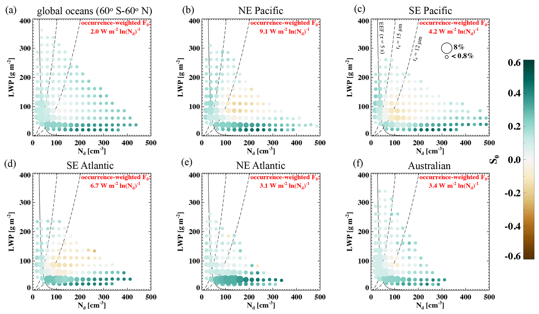
Figure 2 Cloud albedo susceptibility (S₀, colored filled circles) in LWP–N_d variable space, as bin means (bin size of 25 g m⁻² and 25 cm⁻³), for (a) global oceans (60^∘ S–60^∘ N) and 20^∘ × 20^∘ boxes over (b) NE Pacific, (c) SE Pacific, (d) SE Atlantic, (e) NE Atlantic, and (f) Australian stratocumulus regions. The size of the circles indicates the frequency of occurrence of an LWP–N_d bin (reference circle sizes with corresponding occurrence are indicated in panel c). Bins with less than 0.01 % frequency of occurrence (or fewer than 25 samples) are not shown. Isolines of evaporation–entrainment feedback (EEF; phase relaxation timescale of 5 s) and isolines of r_e of 12 and 15 µm based on an adiabatic condensation rate of 2.14 × 10⁶ kg m⁻⁴ (dashed black; commonly used measures of precipitation) are indicated in panel (c). Mean radiative susceptibility (F₀) weighted by the frequency of occurrence of each LWP–N_d bin and the effective cloud frequency (freq_eff, defined in Eq. 1) is printed in red (named occurrence-weighted F₀).

Although different stratocumulus basins have different cloud state distributions in the LWP–N_d variable space, the non-precipitating–brightening and the precipitating–brightening regimes remain rather persistent – that is cloud states to the left of the 12–15 µm isolines and cloud states with LWP <50 g m⁻², respectively. In contrast, cloud states associated with a darkening potential vary from basin to basin, from being almost absent over the NE Atlantic (occurring ∼ 2 % of the time) to occurring ∼ 32 % of the time over the SE Atlantic and ∼ 34 % over the SE Pacific (Fig. 2). This sensitivity of the darkening regime to the ocean basin (discussed further in the following sections) is consistent with a dependence of LWP adjustment on meteorological conditions (e.g., Zhang et al., 2022; Gryspeerdt et al., 2019; Possner et al., 2020). When all marine low clouds are combined in the LWP–N_d space (Fig. 2a), one may conclude a predominant cloud brightening potential and a lack of cloud darkening potential, which is not the case for three of the Earth's major semi-permanent stratocumulus decks (Fig. 2b–d).

To learn how these susceptibility regimes constitute the overall albedo susceptibility of each geographical location, we quantify the frequency of occurrence (Fig. 3) of each susceptibility regime and their contributions to the overall F₀ (Fig. 4) for 5^∘ × 5^∘ oceanic areas globally, based on the sign of S₀ and an r_e of 12 µm (above which clouds are more likely to drizzle) as manifested in the LWP–N_d variable space. Clearly, the three susceptibility regimes have distinct geographical preferences (Figs. 3 and 4). The non-precipitating–brightening regime occurs the most frequently over the shallow, often polluted, stratus/stratocumulus off the coast of continents and tends to dominate the F₀ therein (Figs. 3a and 4a). The precipitating–brightening regime, although occurring over 50 % of the time over most parts of the remote clean oceans and the equatorial eastern Pacific (Fig. 3c), contributes little to the overall F₀ (Fig. 4c) due to the low areal coverage of these often precipitating clouds (disorganized or open-cellular form). In between the geographical preferences of the above two regimes lies the region where the darkening regime (mostly non-raining) becomes the leading contributor to the overall F₀, especially over the SE Pacific and SE Atlantic (Figs. 3b and 4b), where net warming potentials are observed (Fig. 1).

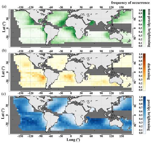
Figure 3 Geographical distribution of the frequency of occurrence of the three susceptibility regimes: (a) non-precipitating–brightening, (b) darkening, and (c) precipitating–brightening. The three regimes are separated based on the sign of S₀ and a r_e of 12 µm in the LWP–N_d variable space for 5^∘ × 5^∘ areas, similarly to Zhang et al. (2022). Only areas with an SLLC frequency of occurrence greater than 0.1 are shown.

Figure 4 As in Fig. 3 but showing radiative susceptibility (F₀).

3.3 Scale-up of the F₀ assessment

The radiative susceptibility derived in this study, F₀, which represents a TOA SW flux response to a unit change in ln (N_d), is equivalent to the radiative sensitivities shown in Bellouin et al. (2020). In order to compare the values from both studies, we scale the aggregated (in LWP–N_d space) F₀ (derived from high-f_c liquid cloud scenes) by an effective cloud frequency (freq_eff) term that takes into account the spatial covariability between F₀ and the frequency of occurrence of high-f_c scenes (scene_freq), which takes the form

$$\begin{array}{}\text{(1)}& {\mathrm{freq}}_{\mathrm{eff}}={\displaystyle \frac{\langle {\mathrm{scene}}_{\mathrm{freq}}\times F_{\mathrm{0}}\rangle }{\langle F_{\mathrm{0}}\rangle }},\end{array}$$

where angle brackets denote spatial averaging. This freq_eff-scaled F₀, which we call the occurrence-weighted F₀, is denoted in Figs. 2 and S6 for global marine low clouds and individual stratocumulus/stratus basins using Aqua and Terra observations, respectively. For global marine low clouds, we obtain an occurrence-weighted F₀ of 2.0 W m⁻² ln(N_d)⁻¹ (freq_eff being 0.061) using Aqua observations and 3.1 W m⁻² ln(N_d)⁻¹ (freq_eff being 0.082) using Terra observations. These are within the bounds provided in Bellouin et al. (2020) based on multiple lines of evidence when one sums up their radiative sensitivities for the Twomey effect (S_𝒩c_𝒩) and the rapid adjustment in LWP (${\mathit{\beta }}_{\ln }\left(\mathcal{L}\right)-\ln \left(\mathcal{N}\right)S_{\mathcal{L},\mathcal{N}}{c}_{\mathcal{L}}$) (using their notations). Bellouin et al. (2020) obtain a cooling sensitivity of ∼ 3.8 W m⁻² ln(N_d)⁻¹ when central values from their Table 4 are used. The difference with the results shown here likely stems from the focus of our study on marine-only high-f_c scenes, whereas Bellouin et al. (2020) integrate evidence from both modeling and satellite studies that cover global warm clouds. When comparing to Bellouin et al. (2020), we do not include the rapid adjustment in cloud cover term, as our study does not consider cloud fraction changes due to N_d perturbations. Also, note the difference in sign convention between the two studies.

4 Distinct distributions of S₀ in two-variable meteorological space at regional scale

Local adjustments of low clouds to aerosol perturbations are strongly dependent on the depth of the stratocumulus-topped MBL (approximated by CTH; e.g., Possner et al., 2020; Toll et al., 2019), the strength of the capping inversion (indicated by LTS), and RH_ft (e.g., Chen et al., 2014; Gryspeerdt et al., 2019). Figures 5–6 show S₀ under different MBL and free-troposphere (FT) states as a function of CTH, LTS, and RH_ft. Globally (60^∘ S–60^∘ N), positive S₀ is found everywhere across the CTH–RH_ft space, with less susceptible conditions occurring under drier FT and intermediate MBL depth (∼ 1.5 km; Fig. 5a). This is consistent with the SW heating and the entrainment feedback arguments (point 2 in Sect. 3.2), in which reduced droplet sizes lead to stronger SW heating and entrainment mixing at cloud tops (Petters et al., 2012; Bretherton et al., 2007; Xue and Feingold, 2006), which is further facilitated by the deeper MBL and the drier air above cloud tops. As clouds become even deeper (> 2 km), the likelihood of precipitation increases, and the cloud brightening potential overwhelms the darkening potential (Fig. 5). Similarly, weak brightening and darkening potential are associated with intermediate MBL depth and high-LTS conditions over global oceans (Fig. 6), as expected, given that LTS anti-correlates with RH_ft over subtropical oceans where large-scale free-tropospheric subsidence prevails.

Figure 5 Mean S₀ under different meteorological conditions, namely free-tropospheric relative humidity (RH_ft; x axis) and cloud-top height (CTH; y axis; a proxy for the marine boundary layer depth), for (a) global oceans (60^∘ S–60^∘ N) and (b) NE Pacific, (c) SE Pacific, (d) SE Atlantic, (e) NE Atlantic, and (f) Australian stratocumulus regions. Bin sizes for CTH and RH_ft are 0.2 km and 10 %, respectively. The size of the square indicates the frequency of occurrence of a meteorological state. Bins with less than 0.1 % frequency of occurrence (or fewer than 100 samples) are not shown.

Figure 6 As in Fig. 5 but for CTH and lower-tropospheric stability (LTS).

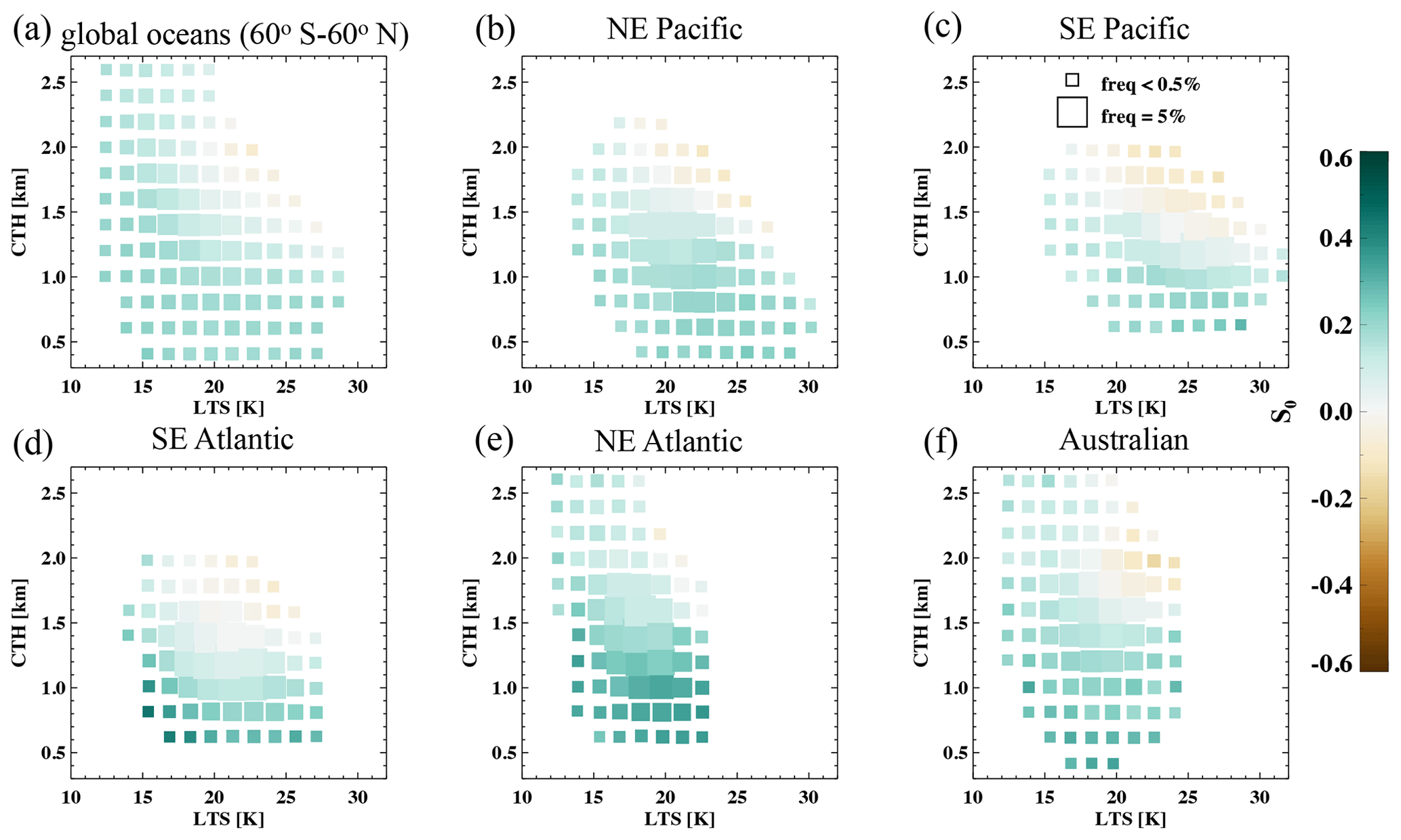
When the stratocumulus regime is singled out (Figs. 5b–f and 6b–f), the S₀ distribution in the two meteorological states is in qualitative agreement with the global analysis; however, cloud darkening (negative S₀) appears under the deep-MBL and dry-FT atmospheric states and more pronouncedly over the SE Pacific stratocumulus deck (Fig. 5c), while weak brightening potential is observed under those conditions over the NE Atlantic (Fig. 5e). This is likely because of the lack of high-LTS conditions over the NE Atlantic (Fig. 6e). The prevalence of weak capping inversions allows the clouds to deepen and potentially precipitate as opposed to entraining and drying with subsiding dry free-tropospheric air, evident over the other four basins (Fig. 6b–d, f). The “disappearance” of the darkening regime over the NE Atlantic, evident both in the LWP–N_d space (Fig. 2) and in the meteorological spaces (Figs. 5–6), is consistent with the findings in Manshausen et al. (2022), where a slight increase in cloud LWP is found in “invisible” ship tracks, which are often identified under weaker cloud-top inversions compared to their surroundings.

Distinct “fingerprints” of S₀, characterized by the sign of S₀ (indicated by the colors) and the frequency of occurrence of meteorological states (indicated by the square sizes), in the large-scale meteorological factor spaces are evident when individual basins are being compared (Figs. 5–6). This manifests in two ways. First, the frequency of occurrence of the FT and MBL conditions varies from basin to basin. For example, deep MBL (>2 km) or humid FT conditions rarely occur under the large-scale subsidence-dominated regions (Fig. 5b–d), compared to the NE Atlantic or the Australian basins (Fig. 5e–f) where high-LTS conditions rarely occur (Fig. 6e–f). Second, different S₀ values, at least in magnitude and in some cases even in sign, are observed across basins under similar conditions (e.g., CTH–RH_ft; Fig. 5). This suggests that cloud states are not necessarily the same under the same CTH–RH_ft conditions, implying that other meteorological factors co-evolve with MBL and FT states differently from region to region, leaving distinct imprints on S₀. In the global analysis (Figs. 5a and 6a), these distinct regional “fingerprints” of S₀–meteorology relationships are not discernible due to the merging of different meteorological regimes.

5 Temporal covariabilities: meteorology, albedo susceptibility, and aerosol conditions

5.1 Meteorological covariability

Four key large-scale meteorological factors evolve and covary distinctly across basins (Fig. 7, right column), leading to markedly different monthly evolutions in F₀ (Fig. 7, left column). Even among regions strongly influenced by large-scale subsidence (Fig. 7a–c), large-scale meteorological conditions vary in magnitude and do not covary the same way temporally (e.g., RH_ft tracks SST except over the SE Atlantic, LTS anti-correlates with SST except over the NE Pacific). As a result of the complex and distinct regional covariability in meteorological conditions, the temporal rise and fall of a single meteorological factor leads to markedly different responses in F₀ across basins. For instance, when LTS peaks over the Australian stratus region, F₀ is at its annual maximum (Fig. 7e, January). In contrast, over the SE Atlantic, the peak LTS season (September–October) corresponds to less susceptible conditions, whereas the most-susceptible clouds of this region are found during a transition of large-scale conditions (i.e., SST decreases and LTS increases, June–July; Fig. 7c), during which the non-precipitating–brightening regime occurs the most frequently (Fig. 8c). Taking CTH as another example, high CTHs (deep MBLs) lead to strong precipitating–brightening over the NE Atlantic, whereas deep MBLs over the SE Pacific show very weak brightening potentials due to relatively high stability and dry FT conditions, in striking contrast to the NE Atlantic (Fig. 7b and d). In other words, when F₀ or S₀ peaks, different combinations of large-scale meteorological conditions occur in different basins. Although certain environmental conditions are known to favor susceptible clouds, e.g., a humid free troposphere and/or strong LTS (Chen et al., 2014), one may not be able to find susceptible clouds under such conditions over some regions due to these regionally distinct meteorological covariabilities.

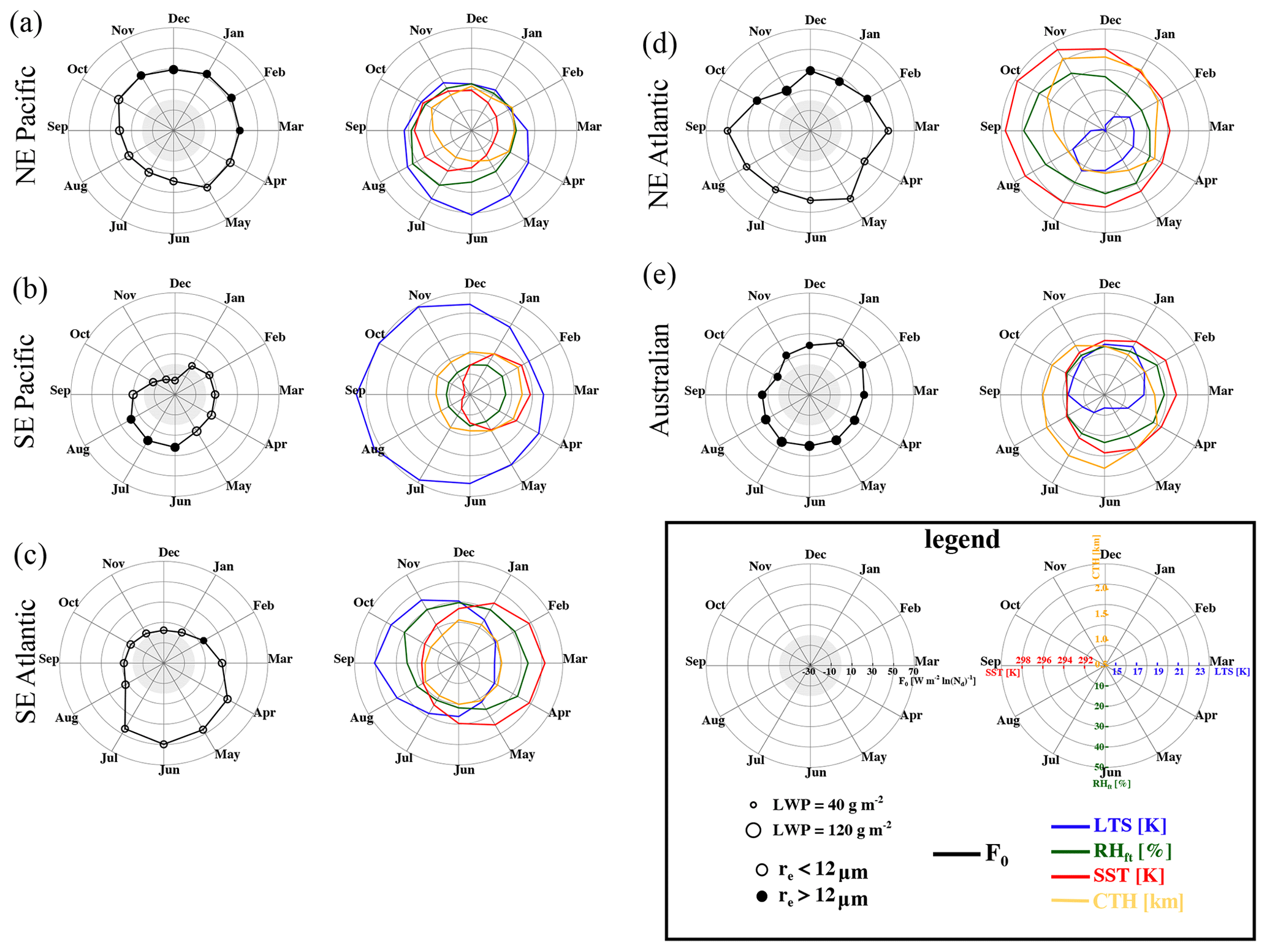
Figure 7 (Left plots of a–e) Monthly mean radiative susceptibility (F₀; black; positive values indicate cooling). The size of the circle indicates monthly mean LWP. Open (closed) circles indicate likely precipitating (non-precipitating) conditions based on r_e=12 µm. (Right plots of a–e) Monthly mean meteorological conditions: LTS (blue), RH_ft (dark green), SST (red), and CTH (orange). Rows (a–e) represent results for the NE Pacific, SE Pacific, SE Atlantic, NE Atlantic, and the Australian stratocumulus regions, respectively.

The covariability among large-scale meteorological factors over the SE Atlantic follows that over the SE Pacific, although the ocean surface is warmer, LTS is weaker, and the FT is moister in general over the SE Atlantic (Fig. 7c). This leads to qualitatively similar F₀ evolutions between the two basins; i.e., high F₀ during austral winter and low F₀ during austral summer. An exception occurs during late fall to winter (June–July), when precipitating clouds over the SE Pacific exhibit relatively weak positive F₀, whereas non-precipitating high-N_d clouds occur and exhibit strong F₀ over the SE Atlantic. This difference can be attributed to an aerosol source that is unique to the SE Atlantic basin in the form of a large amount of biomass burning aerosol that is advected by the co-occurring African easterly jet in the free troposphere during the southern African burning season (June–October; Adebiyi and Zuidema, 2016). The elevated aerosol is likely to be entrained into the MBL during June–July when the FT jet is not yet at its full strength (Zhang and Zuidema, 2021).

Figure 8 Monthly frequency of occurrence of the three susceptibility regimes: precipitating–brightening (blue), darkening (brown), and non-precipitating–brightening (green). Rows (a–e) represent results for the NE Pacific, SE Pacific, SE Atlantic, NE Atlantic, and the Australian stratocumulus regions, respectively.

Among five subtropical stratocumulus/stratus regions, the SE Pacific hosts the least-susceptible conditions overall and is the only basin with monthly mean cloud darkening potential (Fig. 7b). This is consistent with the strongly subsiding (high LTS) and extremely dry free troposphere observed therein, under which entrainment mixing at cloud tops can be extremely effective in reducing cloud LWP (thinning the clouds) and even more so when droplet sizes are reduced due to increasing aerosol. Low clouds over the NE Atlantic indicate the highest cloud brightening potential among the five regions, especially during March–September when the MBL is shallow, and the free troposphere is relatively moist, giving rise to thin, non-precipitating clouds with low LWP and relatively high N_d that exhibit brightening potentials (Fig. 7d). The lowest LTS (weakest subsidence) among the five basins favors cloud deepening (an increase in LWP), leading to the lowest frequency of occurrence of the darkening regime over the NE Atlantic (Fig. 8d). During October–February over the NE Atlantic, when CTH is high (deep MBL), clouds precipitate often, leading to a frequently occurring precipitating–brightening regime (Fig. 8d). Given the deep MBLs, precipitating conditions occur fairly frequently over the Australian stratus region almost throughout the year, except for the January–March period when increasing LTS leads to lower LWP and shallower MBL (Fig. 7e). As a result, the precipitating–brightening regime dominates almost all year round, with the non-precipitating–brightening regime contributing only during austral summer (December–March) (Fig. 8e).

5.2 Albedo susceptibility and aerosol covariability

Albedo susceptibility (S₀), cloud frequency and areal coverage (f_c), incoming solar radiation (SW_dn), and aerosol perturbation (Δln (N_d)) collectively determine the SW flux change at TOA in response to an aerosol perturbation. Mathematically, if these variables covary with each other in time, the temporal mean (indicated by the overbar) of their product,

$$\begin{array}{}\text{(2)}& \mathrm{\Delta }{\mathrm{SW}}_{\mathrm{TOA}}=\stackrel{\mathrm{‾}}{S_{\mathrm{0}}\times f_{\mathrm{c}}\times {\mathrm{SW}}_{\mathrm{dn}}\times \mathrm{\Delta }\ln \left(N_{\mathrm{d}}\right)},\end{array}$$

will be biased if one takes temporal averages before multiplication.

$$\begin{array}{}\text{(3)}& \mathrm{\Delta }{\mathrm{SW}}_{\mathrm{TOA}}^{*}=\stackrel{\mathrm{‾}}{S_{\mathrm{0}}}\times \stackrel{\mathrm{‾}}{f_{\mathrm{c}}}\times \stackrel{\mathrm{‾}}{{\mathrm{SW}}_{\mathrm{dn}}}\times \stackrel{\mathrm{‾}}{\mathrm{\Delta }\ln \left(N_{\mathrm{d}}\right)}\end{array}$$

Deriving S₀ from daily satellite snapshots enables us to resolve these variables temporally, giving us the opportunity to assess the temporal covariability among them and how much it affects the mean (integrated over a long time period) SW flux changes at TOA. This has not been done in previous satellite studies that assess the ERF_aci (effective radiative forcing due to aerosol–cloud interactions; most of them referenced in Bellouin et al., 2020) mainly due to the use of the full temporal span of the dataset to derive a single value (with uncertainty range) for cloud or aerosol susceptibility. Here we assess the impact of temporal covariabilities on time-mean TOA SW flux responses from two perspectives: (a) the ERF_aci per unit anthropogenic emission, equivalent to F₀, and (b) a marine cloud brightening (MCB) experimental scenario in which a prescribed N_d perturbation of 300 cm⁻³ is assumed, a value that might produce sufficient forcing to offset doubled CO₂ according to Wood (2021). We quantify percentage biases, e, calculated as $(\mathrm{\Delta }{\mathrm{SW}}_{\mathrm{TOA}}^{*}-\mathrm{\Delta }{\mathrm{SW}}_{\mathrm{TOA}})/\mathrm{\Delta }{\mathrm{SW}}_{\mathrm{TOA}}$ at each 1^∘ grid point using daily values for each variable and considering a time mean of 8 years (full data temporal range). Note the assessment in (b) is not dependent on the value of the prescribed ΔN_d since percentage biases are being evaluated. Additionally, biases associated with using monthly mean values in $\stackrel{\mathrm{‾}}{S_{\mathrm{0}}\times f_{\mathrm{c}}\times {\mathrm{SW}}_{\mathrm{dn}}\times \mathrm{\Delta }\ln \left(N_{\mathrm{d}}\right)}$ are also evaluated, given that global climate model (GCM) intercomparison projects store monthly mean outputs.

5.2.1 ERF_aci per unit anthropogenic emission

In the first case, the Δln (N_d) term is often estimated by the difference between present-day and historical (pre-industrial) sulfate loading in the MBL (e.g., McCoy et al., 2017; Wall et al., 2022), which is not temporally resolved. Consequently, we only assess the bias associated with the covariability among S₀, f_c, and SW_dn, whose product is essentially F₀. Thus, $F_{\mathrm{0}}=\stackrel{\mathrm{‾}}{S_{\mathrm{0}}\times f_{\mathrm{c}}\times {\mathrm{SW}}_{\mathrm{dn}}}$ and $F_{\mathrm{0}}^{*}=\stackrel{\mathrm{‾}}{S_{\mathrm{0}}}\times \stackrel{\mathrm{‾}}{f_{\mathrm{c}}}\times \stackrel{\mathrm{‾}}{{\mathrm{SW}}_{\mathrm{dn}}}$, where overbars indicate temporal averaging. Globally, $F_{\mathrm{0}}^{*}$ overestimates F₀ by 15 % (i.e., less cooling potential at TOA when covariability is considered by using temporally resolved variables), with the bias non-systematic geographically ($\langle e{\rangle }^{\mathrm{2}}/\langle e^{\mathrm{2}}\rangle \sim \mathrm{0}$) (Table 1). For the five stratocumulus/stratus regions, the overestimation by $F_{\mathrm{0}}^{*}$ is less but varies greatly from basin to basin, 1 % over the NE Atlantic to 14 % over the SE Pacific, suggesting that the degree of covariability among S₀, f_c, and SW_dn varies across basins. It is worth noting that the degree of geographically systematic bias also differs from basin to basin such that 63 % of the grid points over the NE Pacific show a consistent sign in the bias, whereas non-systematic biases are found over the SE Pacific and SE Atlantic. This indicates that S₀, f_c, and SW_dn temporally covary more systematically over the NE Pacific than the other basins. When monthly mean values are used for individual terms in $\stackrel{\mathrm{‾}}{S_{\mathrm{0}}\times f_{\mathrm{c}}\times {\mathrm{SW}}_{\mathrm{dn}}}$, biases decrease globally and at each basin compared to that when 8-year means are used (Table 1), which suggests that monthly means are able to capture some degree of the temporal covariability among these variables. Interestingly, in three of the five basins (SE Pacific, SE and NE Atlantic), the sign of monthly mean biases flips compared to that of 8-year means. This likely indicates that the temporal covariabilities among S₀, f_c, and SW_dn are more pronounced at the monthly timescale. There is no noticeable difference in the degree of geographical systematic bias when monthly mean values are used compared to that when 8-year means are used. Overall, comparing to the other uncertainties associated with estimating ERF_aci, e.g., uncertainties in satellite retrievals and the historical N_d level (Bellouin et al., 2020), biases associated with using monthly means or climatological means do not pose a pressing concern (Table 1).

Table 1 Percentage bias (e) in time-mean F₀ due to temporal covariabilities among S₀, f_c, and SW_dn. e is calculated as $(F_{\mathrm{0}}^{*}-F_{\mathrm{0}})/F_{\mathrm{0}}$. $F_{\mathrm{0}}^{*}$ is calculated using monthly mean and 8-year mean values. Mean of bias, 〈e〉, and the ratio between the squared mean bias, 〈e〉², and the mean squared bias, 〈e²〉, are shown for global oceans and the five stratocumulus regions. Angle brackets denote spatial averaging. Grid points with fewer than 30 samples and outside the 10th and 90th percentiles of e are excluded from the spatial averaging to remove highly uncertain bias calculations.

Figure 9 Same as in Fig. 7 left column and overlaid with monthly mean N_d in blue.

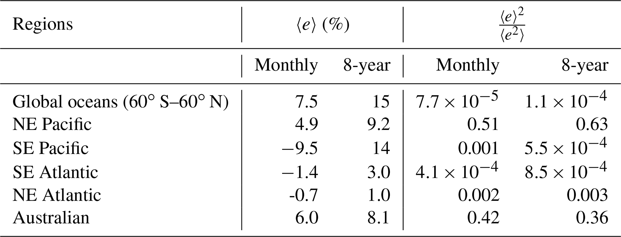
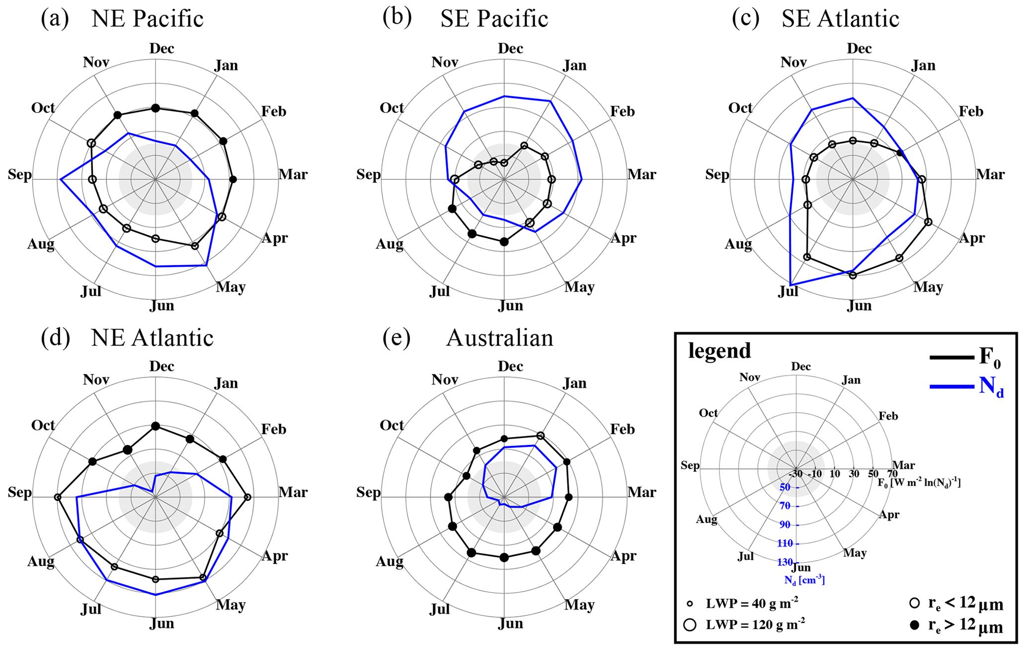
Table 2 As in Table 1 but with the percentage bias, e, calculated as $(\mathrm{\Delta }{\mathrm{SW}}_{\mathrm{TOA}}^{*}-\mathrm{\Delta }{\mathrm{SW}}_{\mathrm{TOA}})/\mathrm{\Delta }{\mathrm{SW}}_{\mathrm{TOA}}$. $\mathrm{\Delta }\ln \left(N_{\mathrm{d}}\right)=\mathrm{\Delta }{N}_{\mathrm{d}}/N_{\mathrm{d}}$, where N_d is temporally resolved and ΔN_d is prescribed to be 300 cm⁻³. Note the value of prescribed ΔN_d does not affect the results as percentage biases are evaluated.

5.2.2 MCB experimental scenario

However, this is not the case when an MCB experimental scenario is considered; here the temporal covariability between radiative susceptibility (F₀) and aerosol conditions (indicated by N_d; Fig. 9) substantially increases the bias in ΔSW_TOA if climatological values of each variable in Eq. (2) are used (Table 2). This covariability is evident in the annual cycles (monthly evolutions) of F₀ and N_d of each stratocumulus basin (Fig. 9). For instance, highly susceptible conditions (indicated by high F₀) co-occur with high background N_d, e.g., over the NE Pacific during May, over the SE Atlantic during July, over the NE Atlantic during May–July, and over the Australian basin during January (Fig. 9). This could lead to a muted ΔSW_TOA, as the higher the background N_d, the lower the Δln (N_d) when a constant ΔN_d is sustained by injecting aerosol particles into the MBL at a fixed rate if such an MCB experiment were attempted. That said, $\mathrm{\Delta }{\mathrm{SW}}_{\mathrm{TOA}}^{*}$ actually underestimates ΔSW_TOA by 35 % globally (Table 2), meaning a stronger TOA SW flux perturbation is expected if the temporal covariability between albedo susceptibility and aerosol is considered. The reason is that, although examples of high-susceptibility high-background-N_d time periods are evident, the overall covariability is dominated by the fact that low-background-N_d conditions (high Δln (N_d)) are usually found under precipitating conditions where clouds exhibit precipitating–brightening potentials (Fig. 9). However, whether sustaining a constant ΔN_d (e.g., 300 cm⁻³) is practical, especially under precipitation prevalent conditions, is outside the scope of this study, and one might need to resolve the diurnal cycle of these variables in order to study that.

Regionally, $\mathrm{\Delta }{\mathrm{SW}}_{\mathrm{TOA}}^{*}$ underestimates ΔSW_TOA as well, ranging from −18 % over the NE Atlantic to −59 % over the SE Pacific. Clearly, biases are much higher in magnitude when the background N_d-dependent Δln (N_d) term is included (Table 2). As mentioned above, percentage biases calculated here are not affected by the prescribed ΔN_d value. When monthly mean values are used, again, the magnitude of bias decreases globally and at each basin (except over the SE Atlantic) compared to that when 8-year means are used (Table 2). Nevertheless, substantial biases (more than 40 %) associated with using monthly means are found over the three major stratocumulus decks. It is worth noting that biases are much more geographically systematic, indicated by the higher $\langle e{\rangle }^{\mathrm{2}}/\langle e^{\mathrm{2}}\rangle$ values, regardless of the degree of averaging (i.e., 8-year or monthly) compared to when Δln (N_d) is not temporally resolved (Table 1). This suggests that temporal covariabilities are more geographically coherent at each basin.

These results stress, first, the necessity of taking the temporal covariability between albedo susceptibility and aerosol condition into account when the background N_d becomes an influencing factor, e.g., for an MCB experimental scenario. Second, the temporal covariability among variables that determine ΔSW_TOA is basin specific, as biases vary in sign and magnitude across basins (Tables 1 and 2). Regardless of the perspectives (ERF_aci or MCB), the most pronounced bias is found over the SE Pacific, suggesting a strong temporal covariability among S₀, f_c, SW_dn, and background N_d therein, whereas the NE Atlantic has the least of such covariability.

6 Discussion

6.1 Diurnal cycle

S₀ and F₀, including the three susceptibility regimes, derived from the morning observations (Terra; Figs. S5–S8) have very similar geographical distributions as those observed in the afternoon (Aqua; Figs. 1–4) except a general shift towards positive S₀, as the darkening regime weakens, and the precipitating–brightening regime is enhanced, with clouds occurring more frequently at higher-LWP states (Fig. S6). One may find more noticeable differences in the cloud-frequency-weighted F₀ geographical distribution (Fig. S5b), especially over the remote part of the SE Pacific stratocumulus deck. This points to another layer of complexity in characterizing and quantifying albedo susceptibility – that is the role of the low-cloud diurnal cycle such that the higher occurrence of low clouds in the morning over the SE Pacific (Garreaud and Muñoz, 2004) enhances the overall brightening potential therein. As a result, Terra observations indicate a slightly higher global mean occurrence-weighted F₀ of 3.1 W m⁻² ln(N_d)⁻¹ (Fig. S6a) compared to 2.0 W m⁻² ln(N_d)⁻¹ for Aqua observations (Fig. 2a). While the qualitative distributions of S₀ in the CTH–RH_ft and the CTH–LTS state spaces remain the same, regardless of the observing time, the morning observations (Figs. S9–S10) indicate a general shift towards positive S₀ as well, which replaces the cloud darkening potentials related to the deep-MBL, dry-FT, and high-LTS conditions (Figs. 5–6) with a weak brightening potential. This, again, stresses the importance of cloud diurnal evolution for S₀ in that the same meteorological conditions may lead to opposing susceptibility regimes (i.e., brightening versus darkening) depending on the time of the day. Except for generally higher cloud LWP and higher F₀, the characterized meteorological covariabilities and the covariability among N_d and F₀ for each stratocumulus basin using the Terra observations (Figs. S11–S13) agree well with those using the Aqua observations (Figs. 7–9). Although the seasonal trend in F₀ is the same between Aqua and Terra observations, the role of the diurnal cycle is manifested in the timing when monthly F₀ peaks (e.g., a lag of a month over the NE Pacific and the SE Atlantic; Figs. S13 and 9).

6.2 Implications

Our work is highly relevant for assessments of the radiative effect of aerosol–cloud interactions for climate applications. The approach we took enables us to reveal distinct S₀–meteorology–aerosol temporal covariabilities over five major subtropical marine stratocumulus/stratus decks while yielding an integrated F₀ that is within the range of the multi-evidence assessment of ERF${}_{\mathrm{aci}}/\mathrm{\Delta }\ln \left(N_{\mathrm{d}}\right)$ in Bellouin et al. (2020) (see Sect. 3.3).

In addition, our findings have direct implications for marine cloud brightening, which has been proposed as a way to mitigate the worst effects of the ongoing global warming crisis by creating more reflective (in the SW) MBL clouds, ideally with expanded areal coverage and prolonged lifetime, through deliberate aerosol injections (Latham et al., 2012). The bright, linear cloud features seen in satellite images, referred to as ship tracks (Coakley et al., 1987), are examples of ideal outcomes of an MCB experiment, and the conditionality of such an outcome on meteorological conditions is one of the key issues underpinning the viability of MCB. This study underscores two key points for the MCB community: (1) understanding or evaluating the impact of meteorology on cloud albedo susceptibility needs to be done at local/regional scales, where meteorological covariability is accounted for; (2) when scaling up the flux perturbation, it is crucial to consider the natural covariability between meteorology and aerosol, to which TOA SW flux responses to aerosol perturbation are sensitive. The latter point stresses the importance of shifting our attention from finding the most-susceptible clouds to finding susceptible clouds that co-occur with favorable conditions (e.g., low background N_d; Fig. 9), as the amount of cooling at TOA due to cloud brightening depends strongly on both the albedo susceptibility and the background N_d (e.g., Wang et al., 2011; Hu et al., 2021).

Although it is quite straightforward nowadays for one to assess how much of an aerosol perturbation is needed to achieve a certain increase in reflective SW using cloud-resolving simulation experiments (e.g., Wang et al., 2011; Chun et al., 2022), these modeling experiments are often state and scale specific (i.e., sensitive to the initial conditions of the simulations) and do not consider the frequency of occurrence of environmental conditions nor the background aerosol concentrations, both of which are crucial for scaling up the responses. Therefore, long-term satellite estimates of albedo susceptibility and flux perturbation that cover the full spatiotemporal frequency of occurrence of environmental conditions worldwide are an important asset for MCB research.

Another key implication of this study is that on the path towards understanding the influence of meteorology on aerosol–cloud interactions, efforts have been made to analyze the entire low-cloud population collectively (globally) (e.g., Chen et al., 2014), while our study suggests such global analyses (e.g., Figs. 2a and 5a) do not always represent what happens regionally. In other words, while certain combinations of meteorological conditions appear to favor susceptible conditions in a global analysis, one may not be able to find such combinations at a given geographical location of interest owing to the regionally distinct meteorological covariability, and it is also likely that a different combination of meteorological conditions hosts the most-susceptible clouds of that location.

7 Concluding remarks

Marine warm cloud albedo susceptibility is derived from satellite-retrieved cloud microphysical properties and radiative fluxes and is sorted by day and geographical location. Geographical distributions of albedo susceptibility and the contributions from three susceptibility regimes (non-precipitating–brightening, darkening, precipitating–brightening) are shown over global oceans (60^∘ S to 60^∘ N). Monthly evolutions in cloud radiative susceptibility, meteorological conditions (from ERA5 reanalysis), and cloud states (LWP and N_d) are shown for five major eastern subtropical stratus/stratocumulus regions (20^∘ × 20^∘) to illustrate the covariability among them and its impact on the response of TOA SW flux. The key findings are as follows.

1. An overall cloud brightening potential (positive S₀) is found in the 8-year means for most global marine warm clouds – most pronounced over subtropical coastal regions, where shallow marine stratocumuli prevail along with relatively high annual mean N_d, and over the equatorial eastern Pacific, where clouds rain more often (Fig. 1).

2. Cloud darkening associated with entrainment-driven negative LWP adjustments offsets the cloud brightening potential over remote parts of the stratocumulus regions where deeper MBLs favor cloud-top entrainment, especially over the SE Pacific and SE Atlantic where darkening overcomes brightening in the 8-year means (Figs. 1 and 3–4).

3. The distinct regional “fingerprints” of S₀ in the LWP–N_d and CTH–RH_ft–LTS variable spaces are indiscernible in the global analysis because different low-cloud and meteorological regimes are merged in a global analysis (Figs. 2 and 5–6).

4. Meteorological conditions have distinct regional covariabilities, leading to markedly different monthly evolutions in F₀ (Fig. 7).

5. The SE Pacific, a region with the driest free-tropospheric conditions and the highest LTS, hosts the least-susceptible clouds exhibiting cloud darkening potential over several months during austral winter. Frequently occurring non-precipitating low-LWP, high-N_d clouds, found in shallow MBLs (March–September) over the NE Atlantic, represent the highest potential radiative responses to N_d perturbations among the five stratocumulus regions (Figs. 7–9).

6. While the qualitative agreement between Terra and Aqua underscores the robustness of our findings, their quantitative disagreement points to the important role of cloud diurnal evolution in determining albedo susceptibility (Figs. S5–S13).

7. Not only do various spatial-temporal averages applied in satellite-based approaches lead to biased S₀ (Feingold et al., 2022), non-negligible biases also exist in ΔSW_TOA estimates, when the regionally distinct temporal covariability between S₀ and background N_d is ignored by using long-term mean values for each variable (Table 2).

8. In the search for the best targets for MCB, should such efforts be attempted, decisions should be made based not only on meteorological regimes, season, and time of day that produce the most-susceptible clouds but also on the background N_d (aerosol loading), which covaries spatiotemporally with the susceptibility of the clouds (Fig. 9).

When the influence of meteorological conditions on low-cloud S₀ is studied, it may seem tempting to try to disentangle effects of individual meteorological factors on S₀ by controlling for the others. Our results, however, indicate that this may not be the best approach since it is the natural covariability among meteorological conditions that dictates the regionally distinct temporal evolution in S₀. These results convey the importance of spatiotemporal variability in S₀ as a basis both for understanding the limitation in scaling up the meteorological influences on the radiative effect of aerosol–cloud interactions from regional to global and for making decisions regarding when, where, and if marine cloud brightening efforts should be attempted.