Biogenic isoprene emissions, dry deposition velocity, and surface ozone concentration during summer droughts, heatwaves, and normal conditions in southwestern Europe

At high concentrations, tropospheric ozone (O₃) deteriorates air quality, inducing adverse effects on human and ecosystem health. Meteorological conditions are key to understanding the variability in O₃ concentration, especially during extreme weather events. In addition to modifying photochemistry and atmospheric transport, droughts and heatwaves affect the state of vegetation and thus the biosphere–troposphere interactions that control atmospheric chemistry, namely biogenic emissions of precursors and gas dry deposition. A major source of uncertainty and inaccuracy in the simulation of surface O₃ during droughts and heatwaves is the poor representation of such interactions. This publication aims at quantifying the isolated and combined impacts of both extremes on biogenic isoprene (C₅H₈) emissions, O₃ dry deposition, and surface O₃ in southwestern Europe.

First, the sensitivity of biogenic C₅H₈ emissions, O₃ dry deposition, and surface O₃ to two specific effects of droughts, the decrease in soil moisture and in biomass, is analysed for the extremely dry summer 2012 using the biogenic emission model MEGANv2.1 and the chemistry transport model CHIMEREv2020r1. Despite a significant decrease in biogenic C₅H₈ emissions and O₃ dry deposition velocity, characterized by a large spatial variability, the combined effect on surface O₃ concentration remains limited (between +0.5 % and +3 % over the continent).

The variations in simulated biogenic C₅H₈ emissions, O₃ dry deposition, and surface O₃ during the heatwaves and agricultural droughts are then analysed for summer 2012 (warm and dry), 2013 (warm), and 2014 (relatively wet and cool). We compare the results with large observational data sets, namely O₃ concentrations from Air Quality (AQ) e-Reporting (2000–2016) and total columns of formaldehyde (HCHO, which is used as a proxy for biogenic emissions of volatile organic compounds) from the Ozone Monitoring Instrument (OMI) of the Aura satellite (2005–2016).

Based on a cluster approach using the percentile limit anomalies indicator, we find that C₅H₈ emissions increase by +33 % during heatwaves compared to normal conditions, do not vary significantly during all droughts (either accompanied or not by a heatwave), and decrease by −16 % during isolated droughts. OMI data confirm an average increase in HCHO during heatwaves (between +15 % and +31 % depending on the product used) and decrease in HCHO (between −2 % and −6 %) during isolated droughts over the 2005–2016 summers. Simulated O₃ dry deposition velocity decreases by −25 % during heatwaves and −35 % during all droughts. Simulated O₃ concentrations increase by +7 % during heatwaves and by +3 % during all droughts. Compared to observations, CHIMERE tends to underestimate the daily maximum O₃. However, similar sensitivity to droughts and heatwaves are obtained. The analysis of the AQ e-Reporting data set shows an average increase of +14 % during heatwaves and +7 % during all droughts over the 2000–2016 summers (for an average daily concentration value of 69 µg m⁻³ under normal conditions). This suggests that identifying the presence of combined heatwaves is fundamental to the study of droughts on surface–atmosphere interactions and O₃ concentration.

1 Introduction

Tropospheric ozone (O₃) plays a critical role in maintaining the oxidative capacity of the troposphere. However, as a high oxidant, it also deteriorates air quality at high concentrations, inducing adverse effects on human and ecosystem health. Both short- and long-term O₃ exposure significantly increase the risk of morbidity and mortality from cardiovascular or respiratory causes (e.g. Jerrett et al., 2009; Nuvolone et al., 2018). It also causes visible damage on plant epidermis and photosynthesis inhibition, thereby seriously threatening vegetation growth (Anand et al., 2021) and crop yields (De Andrés et al., 2012). Tai et al. (2014) estimate that O₃ pollution enhanced by global warming (Representative Concentration Pathway 8.5) could lead to a global crop yield reduction of 3.6 % in 2050.

Tropospheric O₃ is a secondary air pollutant formed by photochemical reaction chains initiated by the oxidation of volatile organic compounds (VOCs) in the presence of nitrogen oxides (NO_x). The VOC $/$ NO_x emission ratio determines the chemical regime of O₃ production at the local scale in a highly nonlinear relationship (Jacob, 1999). Methane (CH₄) and carbon monoxide (CO) are also O₃ precursors in background conditions.

Meteorological conditions are a key driver for O₃ formation and transport (Mertens et al., 2020). Indeed, O₃ production is favoured by warm and sunny conditions, and O₃ peaks therefore occur mainly during summer. The overall objective of this paper is to quantify the variation in surface O₃ concentrations over the Euro–Mediterranean area during extreme weather events of heatwaves and droughts. The Euro–Mediterranean region is often affected by both heatwaves (Russo et al., 2015) and droughts (Spinoni et al., 2015). The intensity and frequency of such events have increased over the last few decades in the region. According to projections based on climate models, these trends could last and worsen over the 21st century (Perkins-Kirkpatrick and Gibson, 2017; Spinoni et al., 2018).

Heatwaves are often associated with high O₃ concentration. For example, Vautard et al. (2005) show that the persistent heatwave of August 2003 led to high O₃ concentration over western Europe for several days (daily maximum above 150 µg m⁻³; spatially averaged). Jaén et al. (2021) report hourly values of O₃ exceeding 250 µg m⁻³ during a shorter heatwave (28–29 June 2019) at a local scale (Barcelona). These values are well above the European Union (EU) recommendation of an 8 h average maximum of 120 µg m⁻³.

Porter and Heald (2019) highlight that, despite a strong correlation between surface temperature and O₃ concentration identified in Europe, this relationship is nonlinear and complex, as it depends on several mechanisms including precursor emissions, reaction rates, and lifetimes in the atmosphere. High temperatures favour emissions of biogenic VOCs (BVOCs), which can induce an increasing formation of O₃ in the case of a NO_x-limited regime, which is found in many areas in the Mediterranean Basin (Richards et al., 2013). Persistent and intense solar radiation also allows long photochemical episodes (Jaén et al., 2021). Since heatwaves in the Mediterranean are often related to a blocking situation of atmospheric systems, stagnant anticyclonic conditions lead to the accumulation of both precursors and O₃ (Otero et al., 2022). Moreover, extreme temperature and high O₃ concentration can cause stomatal closure, thus reducing the dry deposition of O₃, as highlighted by Gong et al. (2020) with the O₃–vegetation feedback.

Droughts also significantly impact atmospheric chemistry through biosphere and atmospheric cycle perturbation (Wang et al., 2017). Drought impact on air pollutants and, more specifically, O₃ is difficult to investigate for several reasons. It is, firstly, related to their characterization. Due to their multiscalar character, droughts can last on timescales ranging from days to months, making their extent difficult to assess (Vicente-Serrano et al., 2010). Moreover, drought definition depends on the type considered (Svoboda and Fuchs, 2016). Meteorological droughts correspond to a rainfall deficit or an excess of evapotranspiration, agricultural ones to soil water shortage for plant growth (soil dryness), and hydrological ones to surface and/or underground flow decrease. Another difficulty is that droughts affect not only the atmosphere but also the land biosphere through soil dryness and plant activity decline (e.g. Vicente-Serrano, 2007; Vicente-Serrano et al., 2013). The variability in O₃ concentration is generally not well represented in chemistry transport models (CTMs) compared to observations, partially because of the lack of interactions between the meteorology, terrestrial biosphere, and atmospheric chemistry (Wang et al., 2017). Uncertainties related to BVOC emission modelling could lead to a BVOC-derived O₃ uncertainty estimated at about 50 % in Europe (Curci et al., 2010). Another major cause of uncertainties concerns the simulation of meteorological conditions.

Meteorological conditions specific to droughts are low relative humidity and low or absent precipitation and cloud cover. The latter leads to an increase in downward solar radiation. Temperature can also be higher during droughts than during normal conditions. Wang et al. (2017) found that drought periods in the United States over 1990–2014 were characterized by temperatures up to 2 ^∘C hotter and radiation 12.4 W m⁻² higher. Their analysis of surface measurements shows a mean enhancement in O₃ concentration of 3.5 ppbv (parts per billion by volume; 8 %), which is explained by enhanced precursor emissions and photochemistry. Finally, large number of O₃ precursors emitted during biomass burning enhanced by droughts and heatwaves can contribute to O₃ pollution peaks (e.g. Hodnebrog et al., 2012).

The development of droughts and heatwaves can be linked (Miralles et al., 2019). For example, through the soil moisture–temperature feedback, droughts can increase heatwave intensity due to a decrease in evapotranspiration and an increase in sensible heat (e.g. Zampieri et al., 2009). It is therefore important to integrate such interactions for the simulation of droughts and heatwaves.

Through soil moisture deficit, droughts can induce considerable adverse effects on the biosphere, leading not only to a decrease in the overall biomass but also of the BVOC emission activity. Guion et al. (2021) report an averaged decrease of ∼ 10 % in leaf area index (LAI) observed by satellite during droughts in southern Europe. Areas of low altitude and vegetation with short root systems are more sensitive. Based on simulations from the Model of Emissions of Gases and Aerosols from Nature (MEGAN; Guenther et al., 2006, 2012) and using MODIS (Moderate Resolution Imaging Spectroradiometer) LAI between 2003 and 2018, Cao et al. (2022) find that vegetation biomass variability in China is a major controlling factor of the interannual variation in BVOC emissions. Furthermore, Emmerson et al. (2019) simulated (also with MEGAN) a reduction in C₅H₈ emissions of 24 %–52 % over southeastern Australia due to soil dryness in summer.

Dry deposition velocity in the Mediterranean depends on both stomatal and non-stomatal conductance (Lin et al., 2020; Sun et al., 2022). Stomatal conductance that can be considerably affected under hot and dry conditions depends on several parameters. As identified by Kavassalis and Murphy (2017), the leaf-to-air vapour pressure deficit that depends on both temperature and relative humidity is a key variable regulating the stomatal conductance. Extreme hot and dry conditions can cause stomatal closure to reduce transpiration. Moreover, the lack of rainfall prevents wet deposition, and plant water stress slows dry deposition. However, there are still large uncertainties about the relationship between the soil moisture and the gas dry deposition (e.g. Clifton et al., 2020b).

Considering the difficulty for models in simulating soil moisture accurately (Cheng et al., 2017) and the uncertainties about plant and BVOC species response to water stress (Bonn et al., 2019), the impact of soil moisture is often dismissed in biogenic emissions and dry deposition schemes used in CTMs. Therefore, knowledge about the respective effect on O₃ remains limited. To evaluate the effects of droughts and heatwaves on surface O₃ in southwestern Europe, the variation in both BVOC emissions and dry deposition as a function of meteorological and hydrological conditions are analysed in this paper including the soil dryness effect.

Agricultural droughts and heatwaves are identified based on the coupled meteorological and land surface vegetation regional model RegIPSL (regional Earth system model of Institute Pierre Simon Laplace) for the 1979–2016 period (Guion et al., 2021). Summers are less affected by drought events (33 % of them) than by heatwaves (97 %). Nevertheless, drought periods are generally much longer than heatwaves (22.3 d vs. 5.8 d). Those two types of extreme weather events can be considerably correlated over the western Mediterranean (temporal correlation R between 0.4 and 0.5).

Atmospheric chemistry is simulated using the regional CHIMERE CTM (Menut et al., 2021) over three selected summers (2012, 2013, and 2014), including the online calculation of biogenic emissions from the MEGANv2.1 model. Simulations are analysed in conjunction with surface O₃ observations from the European surface network Air Quality e-Reporting (https://www.eea.europa.eu/data-and-maps/data/aqereporting-9, last access: 30 July 2021). Concentrations of formaldehyde (HCHO) are used as a proxy for BVOC emissions. HCHO is produced in high yield during the oxidation of hydrocarbons. As an intermediate product of the oxidation of most VOC and being characterized by a short lifetime (about a few hours), HCHO has been used in many studies to infer VOC emissions (e.g. Millet et al., 2006, 2008; Curci et al., 2010). Observations of HCHO total column by the Ozone Monitoring Instrument (OMI) aboard the Aura satellite (Levelt et al., 2006) are used.

The observations and models used for this research are presented in Sects. 2 and 3, respectively. The RegIPSL, CHIMERE, and MEGAN models, as well as the different modelling experiments undertaken, are detailed. Validation of surface O₃, NO₂, and 2 m temperature are presented in Sect. 4. The results (see Sect. 5) are divided into three parts. First, the sensitivity of C₅H₈ emissions, O₃ dry deposition, and surface O₃ concentration to drought effects (biomass decrease and soil dryness) is assessed in Sect. 5.1. Second, the variation in observed and simulated O₃, integrating drought and heatwave effects, is analysed with respect to the variation in troposphere–atmosphere interactions during extreme weather events (see Sect. 5.2). Finally, the number and distribution of days exceeding the EU air quality standard are presented (see Sect. 5.3).

2 Observations

2.1 European surface network of O₃ and NO₂ concentration

The in situ measurements of surface O₃ and NO₂ provided by the European Environment Agency are used (EEA; https://www.eea.europa.eu/data-and-maps/data/aqereporting-9). The Air Quality (AQ) e-Reporting project gathers air quality data provided by EEA member countries as well as European collaborating countries. Merging with the statistics of the AirBase v8 project (2000–2012), AQ e-Reporting offers a multiannual time series of air quality measurement data until 2021, categorized by station types and zones across Europe. Only measurements from stations classified as background and rural are considered for this study.

Thunis et al. (2013) quantify the various sources of uncertainty for O₃ measurements (e.g. linear calibration and ultraviolet photometry) and estimated a total uncertainty of 15 %, regardless of concentration level. There are also considerable uncertainties in the measurements of NO₂. Lamsal et al. (2008) emphasize that the chemiluminescence analyser, the measurement technique primarily found in air quality stations, is subject to significant interference from other reactive species containing oxidized nitrogen (e.g. PAN and HNO₃). This can lead to an overestimation of measured NO₂ concentrations.

2.2 Satellite observations of HCHO total column

The HCHO total column retrieved from the observations of the backscatter solar radiation in the ultraviolet (306 and 360 nm) by the OMI/Aura instrument are used as a quantitative proxy for BVOC emissions. OMI has an Equator-crossing time at 13:45 LT (local time)​​​​​​​ on the ascending node, about 14.5 revolutions per day, and a swath width of 2600 km, allowing daily global coverage (Levelt et al., 2006, 2018).

Uncertainties in the HCHO retrieval are significant, varying between 30 % (pixels with high concentrations) and 100 % (with low concentrations), mainly due to cloud and aerosol scattering along the field of view (González Abad et al., 2015). Satellite retrievals of HCHO have been shown to have systematic low mean bias (20 %–51 %) compared to aircraft observations (Zhu et al., 2016).

For this reason, we chose to focus on the relative difference in total HCHO during droughts and heatwaves (no correction factor has been applied). In order to quantify the uncertainty in the HCHO anomalies obtained, the analysis has been performed using two products. We primarily use the OMHCHOd level 3 product (Chance, 2019), which provides the HCHO total column with a spatial resolution of 0.1^∘ × 0.1^∘. For comparison, the level 2 retrieval by the Belgian Institute for Space Aeronomy (BIRA) is also used (De Smedt et al., 2015, hereafter referred to as OMI-BIRA). Both products are included in the intercomparison conducted by Zhu et al. (2016).

Only observations with a cloud fraction less than 0.3, a solar zenith angle less than 70^∘, and a vertical column density within the range of −0.8 × 10¹⁵ and 7.6 × 10¹⁵ molec. cm⁻² are selected in order to minimize OMI row anomalies, following Zhu et al. (2017). For a suitable comparison with model simulations, HCHO data were regridded on the Med-CORDEX (Coordinated Regional Climate Downscaling Experiment over the Mediterranean) domain using a bilinear method.

2.3 In situ observations of 2 m temperature, C₅H₈ surface concentration, and O₃ dry deposition flux

To complete the validation of our simulations, several observational data sets are added to our study. First, in situ observations of temperature at 2 m above the surface (T_2 m) from the E-OBS data set (Cornes et al., 2018) are used to validate the simulated temperature by the Weather Research and Forecasting (WRF) model (Skamarock et al., 2008). The E-OBS gridded product, with a resolution of 0.25^∘ × 0.25^∘, was regridded to the Med-CORDEX domain (see Sect. 3.1.1).

Second, flux measurements are used for comparison with the different modelling experiments carried out to analyse the sensitivity of biogenic C₅H₈ emissions and O₃ deposition to the effects of biomass decrease and soil dryness. However, there are few flux measurements available that cover at least several weeks during summer 2012. The Ersa station (FR0033R), located at Cape Corsica in France (42.97^∘ N, 9.38^∘ E), is used to assess the surface concentration of C₅H₈ measured by a steel canister instrument at 4.0 m above the surface. The data are provided by the EBAS infrastructure (https://ebas.nilu.no/, last access: 14 April 2022).

Dry deposition flux measurements of O₃ are also used at one station. This is the Castel Porziano station (IT-Cp2), located in the Lazio region of Italy (41.70^∘ N, 12.36^∘ E), measuring at 14.9 m above the surface (eddy covariance technique). A full description of the measurement data is provided in Fares et al. (2013). The data were downloaded from the European Fluxes Database Cluster (EFDC; http://www.europe-fluxdata.eu/, last access: 16 October 2022).

3 Models

3.1 RegIPSL (WRF-ORCHIDEE)

3.1.1 Model description

The regional WRF-ORCHIDEE model (RegIPSL) couples the land surface model of ORCHIDEE (ORganising Carbon and Hydrology In Dynamic EcosystEms; Maignan et al., 2011) and the meteorological model WRF. ORCHIDEE is composed of three modules, namely SECHIBA, which simulates the water and energy cycle, STOMATE, which resolves the processes of the carbon cycle, allowing therefore an interactive phenology, and, finally, LPJ, which computes the competition between the plant functional types (PFTs). However, the LPJ module is not used for this research.

The RegIPSL model has been used following the recommendation of the Med-CORDEX initiative (Ruti et al., 2016). On a Lambert conformal projection, the domain covers the Euro–Mediterranean region with a spatial resolution of 20 km. The full description of the configuration used with RegIPSL is presented in Guion et al. (2021).

The performed Med-CORDEX simulations over the 1979–2016 period have been evaluated against surface observations of temperature and precipitation, demonstrating that it is suitable for research on droughts and heatwaves (Guion et al., 2021).

3.1.2 Indicators of drought and heatwave

Based on simulations performed by the RegIPSL model, we identified heatwaves and agricultural droughts over the Euro–Mediterranean region using indicators of extreme weather events (Guion, 2022; data access: https://thredds-x.ipsl.fr/thredds/catalog/HyMeX/medcordex/data/Droughts_Heatwaves_1979_2016/catalog.html, last access: 14 April 2022).

Following the approach of Lhotka and Kyselý (2015), we computed the percentile limit anomalies (PLAs) of temperature 2 m above the surface (PLA_T2 m), for heatwave detection, and of soil dryness (PLA_SD), for agricultural drought detection. The soil dryness is computed as the complement of the soil wetness index, which is described in ORCHIDEE as the ratio between the soil moisture and the accessible water content.

For each cell of longitude (i) and latitude (j) of the domain, the monthly distribution of the 2 m temperature/soil dryness is normalized, and the 75th percentile is computed (p=0.75). The daily ${\mathrm{PLA}}_{T\mathrm{2}\mathrm{m}/\mathrm{SD}}$ indicator (Eq. 1) is equal to the daily deviation ($\mathrm{d}{X}_{i,j,d}$) between the reference variable ($X_{i,j,d}$) and the corresponding monthly percentile ($X_{i,j,m}^p$). A heatwave/drought is identified when the daily ${\mathrm{PLA}}_{T\mathrm{2}\mathrm{m}/\mathrm{SD}}$ is positive for 3 consecutive days.

$$\begin{array}{}\text{(1)}& \mathrm{d}{X}_{i,j,d}=X_{i,j,d}-X_{i,j,m}^p.\end{array}$$

The chosen percentile for the detection of extreme weather events is generally higher, between the 80th and 95th percentile (e.g. Stéfanon et al., 2012). We chose the 75th percentile in this study for a larger population. As a result, events detected here cover not only extreme events but also periods that are significantly drier and warmer than normal conditions.

PLA_T2 m was calculated based on 2 m temperature observations (E-OBS data set) in Guion et al. (2021). Although the intensity of the heatwaves was slightly overestimated with the Med-CORDEX simulations (+0.16 ^∘C for the mean bias and +0.50 ^∘C for the maximum bias), their temporal correlation with observations was high (R coefficient of about 0.9 over the whole Mediterranean).

3.1.3 Soil water stress for plants

The soil water stress (SWS) calculated by RegIPSL is used to describe the water stress for plant transpiration and photosynthesis (de Rosnay et al., 2002). It is an index varying between 0 (plants fully stressed) and 1 (not stressed) that takes into account the water transfer between the soil layers along root profiles (11 layers in the version of ORCHIDEE used here). For each PFT (p), soil class (s), and soil layer (v), it is computed as follows:

$$\begin{array}{}\text{(2)}& {\mathrm{SWS}}_{p,s}={\displaystyle \frac{{\mathrm{SM}}_{p,s,v}-{\mathrm{SMw}}_{p,s,v}}{{\mathrm{SMnostress}}_{p,s,v}-{\mathrm{SMw}}_{p,s,v}}}\times {\mathrm{nroot}}_{p,s,v},\end{array}$$

where SM is the soil moisture (liquid phase), SMw is the level at wilting point, SMnostress is the level at which SWS reaches 1, and nroot is the normalized root length fraction in each soil layer (between 0 and 1). There are three soil classes to avoid competition for water uptake, namely bare soil, soil with short root systems, and soil with long ones.

3.2 CHIMERE

3.2.1 Model description and configuration

The CHIMERE v2020r1 Eulerian 3-dimensional regional CTM (Menut et al., 2021) computes gas-phase chemistry and aerosol formation, transport, and deposition. It can be guided by precalculated meteorology (offline simulation) or used online with the WRF regional meteorological model (Skamarock et al., 2008), including the option with the direct and indirect effects of aerosols. In this study, we chose to use the online version of CHIMERE but without any aerosol effects in order to reduce the calculation time and to isolate possible feedbacks.

Here, the reduced scheme MELCHIOR2 (Derognat, 2003) is used for gas-phase chemistry (44 species; almost 120 reactions). The aerosol module includes aerosol microphysics, secondary aerosol formation mechanisms, aerosol thermodynamics, and deposition, as detailed in Couvidat et al. (2018) and Menut et al. (2021). The photolysis rates are calculated online using the Fast-JX module version 7.0b (Bian and Prather, 2002), which accounts for the radiative impact of aerosols.

The WRF model used with CHIMERE, which has a different configuration from the RegIPSL model (Guion et al., 2021), has 15 vertical layers, from 998 up to 300 hPa. The physics interface for the surface is provided by the Noah land surface model. The aerosol-aware Thompson scheme (Thompson and Eidhammer, 2014) is used for the microphysics parameterization. Horizontal and vertical advection are based on the scheme of Van Leer (1977). The reanalysis meteorological data for the initial and boundary conditions are provided by the National Centers of Environmental Prediction (NCEP). The physical and chemical time steps are, respectively, 30 and 10 min.

The simulations have been performed for June, July, and August (JJA, with a 5 d spinup) of the years 2012, 2013, and 2014 over two nested simulation domains (Fig. 1). The large domain covers northern Africa and Europe at 60 km horizontal resolution (EUMED60; 164 × 120 cells), and the small domain is close to that of Med-CORDEX but smaller; it covers the western Mediterranean region at 20 km horizontal resolution (Med-CORDEX; 222 × 93 cells). The area studied in more detail in the following is southwestern Europe (35–46^∘ N, 10^∘ W–20^∘ E).

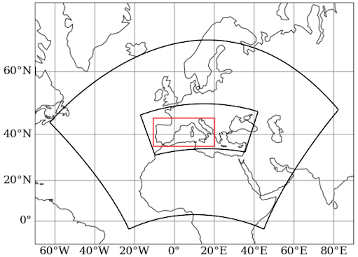
Figure 1 Domains used for the CHIMERE simulations. EUMED60 at 60 km resolution is the large domain, and the smaller nested domain is Med-CORDEX at 20 km resolution. The southwestern Europe region studied here is shown in red.

Chemical boundary conditions for the larger domain are provided by the climatology from the global CTM LMDZ4-INCA3 (Hauglustaine et al., 2014), for trace gases and non-dust aerosols, and from the GOCART model (Chin et al., 2002), for dust.

The biogenic emissions are calculated online by the MEGAN model (see Sect. 3.2.2). Sea salts and dimethyl sulfide marine emissions are calculated online using the scheme of Monahan (1986) and Liss and Mervilat (1986), respectively. Mineral dust emissions are also calculated online (Marticorena and Bergametti, 1995; Alfaro and Gomes, 2001). Consistent with the WRF model, the land cover classification used for the calculation of biogenic and dust emissions is from the United States Geological Survey (USGS) land cover database (http://www.usgs.gov, last access: 14 April 2022). The biomass burning emissions from the APIFLAME v2.0 model (Turquety et al., 2020) are used. The anthropogenic surface emissions are derived from the European Monitoring and Evaluation Programme (EMEP) database at 0.1^∘ × 0.1^∘ resolution (https://www.ceip.at/webdab-emission-database, last access: 14 April 2022) for the year 2014. The inventory was preprocessed by the emiSURF program in order to calculate hourly emissions fluxes on the CHIMERE grid and the period of simulations (https://www.lmd.polytechnique.fr/chimere/2020_getcode.php, last access: 14 April 2022).

3.2.2 MEGAN and the soil moisture factor

BVOC emissions were computed using the MEGAN model v2.04 (Guenther et al., 2006), including several updates from the version 2.1 (Guenther et al., 2012). It is used online in the CHIMERE model at an hourly time step. Emission fluxes are calculated based on emission factors at canopy standard conditions that are defined as 303 K for the air temperature (T), 1500 µmol m⁻² s⁻¹ for the photosynthetic photon flux density (PPFD) at the top of the canopy, 5 m² m⁻² for the LAI, and a canopy composed of 80 % mature, 10 % growing, and 10 % old foliage. Environmental conditions are taken into account using activity factors (γ) that represent deviations from the canopy standard conditions, so that the emission rate (ER; µg m⁻² h⁻¹) for a given species i is calculated in each model grid cell as follows:

$$\begin{array}{}\text{(3)}& {\mathrm{ER}}_i={\mathrm{EF}}_i\cdot {\mathit{\gamma }}_{\mathrm{LAI}}\cdot {\mathit{\gamma }}_{\mathrm{PPFD},i}\cdot {\mathit{\gamma }}_{T,i}\cdot {\mathit{\gamma }}_{\mathrm{Age},i}\cdot {\mathit{\gamma }}_{\mathrm{SM},i}\cdot {\mathit{\gamma }}_{{\mathrm{CO}}_{\mathrm{2}},i}\cdot {\mathit{\rho }}_i,\end{array}$$

where EF is the emission factor (µg m⁻² h⁻¹) provided by the MEGAN model, and ρ is the production/loss term within canopy that is assumed to be equal to 1.

γ_LAI is the activity factor based on LAI observations from the MODIS MOD15A2H product (Myneni et al., 2015) improved by Yuan et al. (2011) (http://globalchange.bnu.edu.cn/research/lai, last access: 14 April 2022). This improvement is undertaken with a two-step integrated method, where (1) the modified temporal spatial filter is used to fill the gaps and replace low-quality data with consistent ones, and (2) the TIMESAT (a program for analysing the time series of satellite sensor data) Savitzky–Golay filter is applied to smooth the final product. The temporal resolution is 8 d.

γ_PPFD, γ_T, and γ_Age are the activity factors accounting for light, temperature, and leaf age, respectively. They are calculated in MEGAN using meteorological variables from the WRF model. The activity factors accounting for the soil moisture (γ_SM) and CO₂ concentration (${\mathit{\gamma }}_{{\mathrm{CO}}_{\mathrm{2}}}$) are applied on C₅H₈ species only. ${\mathit{\gamma }}_{{\mathrm{CO}}_{\mathrm{2}}}$ is fixed (CO₂ concentration at 395 ppm – parts per million), and γ_SM depends on the deviation between the soil wetness and a fixed wilting point, which is computed as follows:

$$\begin{array}{}\text{(4)}& \left\{\begin{array}{ll}{\mathit{\gamma }}_{\mathrm{SM}}=\mathrm{1}& \text{if }\mathit{\theta }>{\mathit{\theta }}_{\mathrm{1}}\\ {\mathit{\gamma }}_{\mathrm{SM}}=\frac{(\mathit{\theta }-{\mathit{\theta }}_{\mathrm{w}})}{\mathrm{\Delta }{\mathit{\theta }}_{\mathrm{1}}}& \text{if }{\mathit{\theta }}_{\mathrm{w}}<\mathit{\theta }<{\mathit{\theta }}_{\mathrm{1}}\\ {\mathit{\gamma }}_{\mathrm{SM}}=\mathrm{0}& \text{if }\mathit{\theta }<{\mathit{\theta }}_{\mathrm{w}},\end{array}\right.\end{array}$$

where θ is the soil wetness (volumetric water content; in m³ m⁻³), θ_w is the wilting point (level from which plants cannot extract water from the soil; in m³ m⁻³), Δθ₁ is equal to 0.04 (empirical parameter), and θ₁ is the sum of θ_w and Δθ₁. θ values (third layer; 60 cm depth) are provided by the WRF-Noah land surface model (Ek et al., 2003; Greve et al., 2013). θ_w values are computed over the domain (Fig. S1 in the Supplement) using tabulated values from Chen and Dudhia (2001) that are soil type specific and parameterized on Noah soil wetness values. These values are spatialized using the soil texture map provided by the USGS (STATSGO-FAO product). However, emission response to drought is very sensitive to the wilting point (Müller et al., 2008). Y. Wang et al. (2021) computed a relative difference in biogenic emissions varying between 50 % and 90 %, depending on the wilting point values.

Based on a comprehensive data set of in situ measurements of C₅H₈ emissions, Bonn et al. (2019) computed an activity factor of soil moisture as a function of the soil water availability. The fitted function is in relatively good agreement with the γ_SM algorithm in MEGAN.

As an alternative, Jiang et al. (2018) propose using an activity factor of soil moisture that integrates the soil water stress for plant photosynthesis. Below a critical value (fixed here at 0.5), the activity factor using SWS from RegIPSL (γ_SWS) decreases linearly as follows:

$$\begin{array}{}\text{(5)}& \left\{\begin{array}{ll}{\mathit{\gamma }}_{\mathrm{SWS}}=\mathrm{2}\mathrm{SWS}& \text{if }\mathrm{SWS}\le \mathrm{0.5}\\ {\mathit{\gamma }}_{\mathrm{SWS}}=\mathrm{1}& \text{if }\mathrm{SWS}>\mathrm{0.5}.\end{array}\right.\end{array}$$

The different soil wetness functions presented here will be subject to dedicated simulations for comparison.

Soil NO emissions are also included in the different simulations. Emission factors are based on the European soil emission inventory (Stohl et al., 1996), which includes contributions from both forests and agricultural soils. Due to the strong temperature dependence, activity factors of soil NO are processed as for biogenic emissions in the MEGAN model. However, no dependence on soil moisture was parameterized.

3.2.3 Dry deposition scheme

Dry deposition in CHIMERE is resolved online using a canopy resistance approach, based on the scheme of the EMEP model (Wesely, 1989; Emberson et al., 2000; Simpson et al., 2003, 2012). Canopy resistance is calculated (Eq. 6) from stomatal conductance (g_sto), which increases proportionally with LAI, and the bulk non-stomatal conductance (G_ns). g_sto varies between a maximum (g_max) and minimum (g_min) daytime stomatal conductance (mmol O₃ m⁻² s⁻¹), depending on a series of meteorological conditions represented by factors of relative conductance (f). The parameters used to calculate these factors vary with the land cover (lc) and the seasonality. Because the land cover classes used in the dry deposition scheme are different from the one used in CHIMERE (USGS), a matrix of conversion is applied.

$$\begin{array}{}\text{(6)}& \begin{array}{rl}{g}_{\mathrm{sto}}& =g_{\max ,\mathrm{lc}}\cdot f_{\mathrm{phen},\mathrm{lc}}\cdot f_{\mathrm{light},\mathrm{lc}}\\ & \cdot max\left(g_{\min ,\mathrm{lc}},(f_{\mathrm{temp},\mathrm{lc}}\cdot f_{\mathrm{VPD},\mathrm{lc}}\cdot f_{\mathrm{SWS},\mathrm{lc}})\right),\end{array}\end{array}$$

where f_X are factors of relative conductance determined by the leaf/needle age (X=phen), irradiance (X=light), temperature (X=temp), leaf-to-air vapour pressure deficit (X=VPD), and the soil moisture (X=SWS). Environmental variables required for f_X factors are from the WRF model, except for f_SWS that is based on SWS from RegIPSL. f_SWS, for which the calculation is the same as γ_SWS, follows the parameterization suggested by Simpson et al. (2012) for the stomatal conductance.

G_ns depends on three resistances, namely the external leaf uptake, the ground surface, and the in-canopy resistance. The external leaf uptake resistance is fixed at 2500 s m⁻¹, the ground surface resistance is estimated from tabulated values (PFT specific), and the in-canopy resistance varies with the surface area index which is expressed in terms of LAI. The LAI used in the dry deposition scheme is parameterized (with no interannual variation). Information on phenology and biomass variation for each land cover type was collected from several studies in Emberson et al. (2000).

3.3 Modelling experiments

The years 2012, 2013, and 2014 were selected for the large diversity of hydroclimatic conditions and the availability of O₃ observations over the study area. During summer 2012, southwestern Europe was affected by severe droughts (PLA_SD>0.1 of soil dryness) and heatwaves (PLA_T2 m>1.5 ^∘C; Fig. S2). The summer of 2013 was wet in the Iberian Peninsula, while summer 2014 was wet in Italy and the Balkans. A few heatwaves occurred in summer 2013 over southern France, northern Italy, and northern Spain. Summer 2014 was colder (PLA_T2 m of −4.0 ^∘C) for the entire study area. The analysis method we propose here is divided into two steps.

Table 1 Name, description, and aim of the simulations launched with the CHIMERE model on the nested Med-CORDEX domain for the summers of 2012, 2013, and 2014.

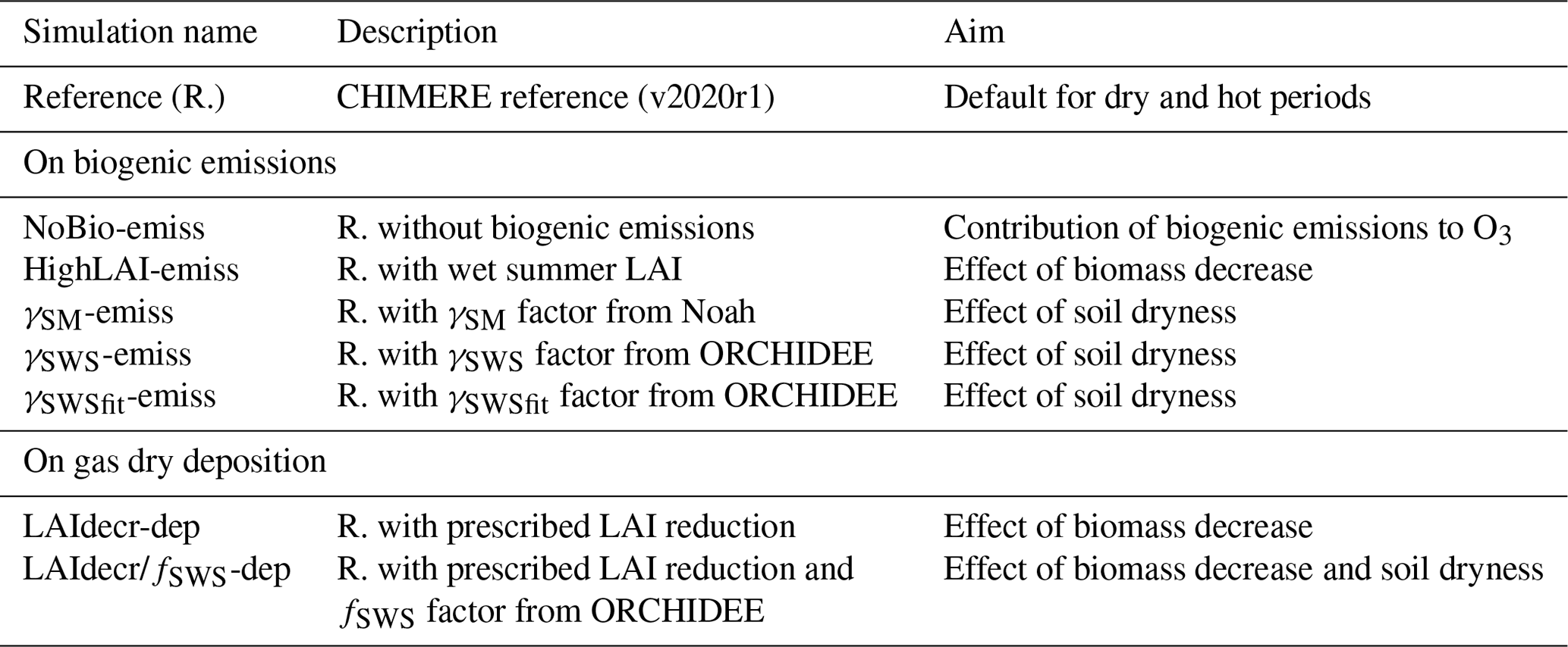
First, the focus is on drought effects (biomass decrease and soil dryness) that are generally poorly represented in modelling experiments over summer 2012. Several experiments are conducted on the Med-CORDEX domain in order to analyse the sensitivity of simulated C₅H₈ emissions, O₃ dry deposition, and surface O₃ concentration to drought effects. Table 1 summarizes the CHIMERE simulations conducted. The “Reference (R.)” simulations include all the emissions as defined in Sect. 3.2.1 but without accounting for the soil moisture factor in the emission scheme of MEGAN and deposition one of CHIMERE. A simulation with no biogenic emissions is also performed (“NoBio-emiss”) to estimate their relative contribution to O₃ concentration.

The LAI used in the emission scheme of MEGAN is year dependent (MODIS observations). To evaluate the effect of biomass decrease by droughts, a simulation with LAI corresponding to a wet summer was used (“HighLAI-emiss”). Summer 2012, which was affected by an important biomass decrease over most of the study area (Fig. S3), has been simulated with the LAI of the wet summer of 2014 (higher than the 2012–2014 mean).

The LAI database used in the dry deposition scheme of CHIMERE does not vary with the year, so the biomass decrease during the summer 2012 is not reflected. In order to evaluate the importance of this effect, a simulation (“LAIdecr-dep”) with a LAI decrease of 5 % for forests and 20 % for grass and crops (close to the variations observed in 2012; Fig. S3) has been conducted.

The effect of soil dryness for the BVOC emissions is evaluated using the following three different approaches:

• γ_SM from WRF-Noah in MEGAN (“γ_SM-emiss” experiment),

• γ_SWS from RegIPSL in MEGAN (“γ_SWS-emiss” experiment), and

• γ_SWSfit from RegIPSL in MEGAN (“γ_SWSfit-emiss” experiment). The fitted function of Bonn et al. (2019) is applied on the SWS as follows:

  $$\begin{array}{}\text{(7)}& \begin{array}{rl}{\mathit{\gamma }}_{\mathrm{SWSfit}}& =\exp \left(-\exp \left(\mathrm{0.056}\cdot \exp \left(\mathrm{1}\right)\right.\right.\\ & \left.\left.\cdot \left(-\mathrm{2.3}-\mathrm{SWS}\right)+\mathrm{1}\right)\right).\end{array}\end{array}$$

The soil dryness effect on the dry deposition is evaluated using the f_SWS from RegIPSL in CHIMERE (“f_SWS-dep” experiment).

Second, based on a simulation configuration integrating all drought and heatwave effects (γ_SWSfit-emiss and LAIdecr/f_SWS-dep in the same experiment, hereafter called the “all-emiss-dep” experiment), the variation in C₅H₈ emissions, O₃ dry deposition velocity, and surface O₃ concentration is analysed over the summers of 2012, 2013, and 2014. In order to compare isolated and combined extreme events with normal conditions, we used a cluster approach based on the PLA_T2 m and PLA_SD indicators.

4 Validation of surface O₃, NO₂, and T_2 m

Simulated surface O₃ and NO₂ concentrations by CHIMERE were compared to the EEA observations, while simulated T_2 m by the WRF model was compared to the E-OBS observations (Cornes et al., 2018). Table 2 presents the mean validation scores of the reference simulations over southwestern Europe for summer 2012. Validation scores of O₃ and NO₂ are very similar for the summers of 2013 and 2014.

Table 2 Comparisons between observed and simulated surface O₃ concentration, NO₂ concentration, and 2 m temperature, averaged over southwestern Europe during summer 2012, for the reference CHIMERE simulation.

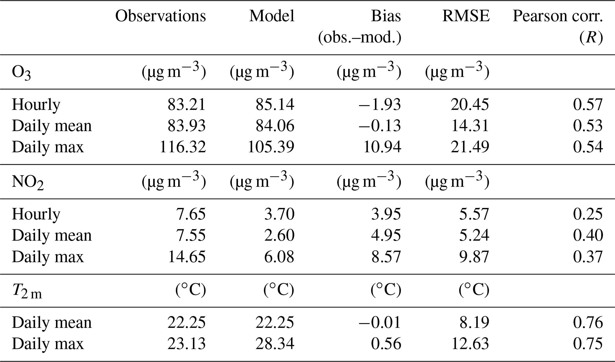
The simulated surface O₃ is slightly higher than the observations for hourly and daily mean values (observation–model, or obs.–mod, bias of −1.93 and −0.13 µg m⁻³) and lower for the daily maximum values (+10.94 µg m⁻³). The simulated diurnal cycle is lower than the observed one because CHIMERE overestimates the daily minimum and underestimates the maximum. The temporal correlation (R, Pearson's coefficient) varies between 0.53 in the daily mean and 0.57 in the hourly mean. The spatial distribution of bias and the correlation scores of the daily maximum values for each summer is shown in the Supplement (Fig. S4). The highest bias (> +25 µg m⁻³) and lowest correlations (R of about 0.2) are obtained near large urban areas (e.g. Madrid and Milan), which may be less well represented in the model, even if the stations are classified as rural background. There are substantial uncertainties related to the NO_x $/$ VOC emissions in (peri-)urban areas.

These O₃ scores show an overall agreement with those calculated by Gaubert et al. (2014) and Menut et al. (2021) over Europe. The averaged daily maximum bias and correlation coefficients computed are slightly higher and lower, respectively, in this study mainly because the area is limited to southwestern Europe. Due to the multiple sources of O₃ precursors and favourable temperature and light conditions, the Mediterranean is identified as a region of important uncertainty for modelling O₃ concentration (Richards et al., 2013).

Validation scores are also computed for the surface NO₂ using the EEA observations, with a different distribution of stations that for O₃. In agreement with the results of Menut et al. (2021), CHIMERE underestimates NO₂ concentrations (+4.95 µg m⁻³ in the daily mean and +8.57 µg m⁻³ in the daily maximum) compared to the EEA observations. Interference from other oxidized nitrogen species in the chemiluminescence analyser (e.g. Lamsal et al., 2008) may explain the constant underestimation compared to observations. The mean temporal correlation coefficients do not exceed 0.4. These low validation scores may also be linked to the emission inventory used in addition to the meteorological conditions (boundary layer height representation in particular). As a major O₃ precursor, part of the uncertainty in this study is directly related to NO₂ emissions and concentrations.

Finally, as a critical variable for simulating diurnal and seasonal O₃ concentrations, T_2 m values have been compared to the E-OBS observations. Averaged over southwestern Europe, the bias is close to 0 ^∘C ,while the RMSE is significant (8.19 ^∘C in the daily mean and 12.63 ^∘C in the daily maximum). The spatial distribution of the bias presents large variations (Fig. S4). The daily maximum T_2 m is overestimated in the southern Mediterranean (up to 5 ^∘C), compared to observations, while it is underestimated in the northern part (up to 5 ^∘C). Nevertheless, the averaged scores of the temporal correlation are high (around 0.75). Even if such validation scores are close to those found in the scientific literature (e.g. Panthou et al., 2018), the temperature uncertainties significantly contribute to those of the O₃ simulated by CHIMERE.

5 Results

5.1 Sensitivity to soil dryness and biomass decrease effects

The sensitivity analysis to soil dryness and biomass decrease effects is focused on summer 2012, as droughts mainly occurred during this year (over the 2012–2014 period). Most of southwestern Europe was affected by a biomass decrease in 2012 (compared to the wet summer of 2014), except for eastern Spain. The LAI difference between summer 2012 and 2014 can reach −30 % over central Italy (Apennines region), corresponding to a mean decrease of 0.5 m² m⁻² (Fig. S3).

C₅H₈ is the main contributor to the total mass of BVOCs emitted (70 %) in our study area, followed by the model species APINEN (13 %, including, e.g., α-pinene and sabinene).

5.1.1 C₅H₈ emissions

Figure 2a shows the daily mean C₅H₈ emissions in southwestern Europe for summer 2012 simulated by the MEGAN model (reference simulation). The spatial distribution of C₅H₈ over the Mediterranean is heterogeneous, ranging from areas of zero or low emissions ($\sim \mathrm{1}\times {\mathrm{10}}^{-\mathrm{3}}$ g m⁻² h⁻¹) to high-emitting areas ($\sim \mathrm{1.5}\times {\mathrm{10}}^{-\mathrm{3}}$ g m⁻² h⁻¹), such as in the Balkans, Apennines, Sierra Morena, Sardinia, and central Portugal. Similar spatial distributions were found for APINEN model species. Differences in spatial patterns among species depend on the variation in emission factors over the land cover classes.

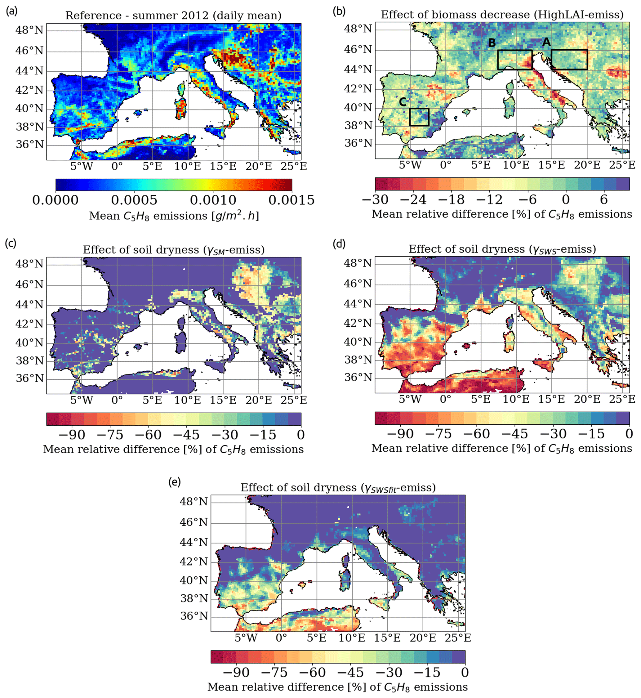
Figure 2 Summer mean (June–August, JJA) of the daily mean C₅H₈ emissions (g m⁻² h⁻¹) for 2012 from the reference simulation (a). Mean relative difference (%) in C₅H₈ emissions due to the biomass decrease and soil dryness. The relative difference is computed between the reference and HighLAI-emiss simulation to quantify the biomass decrease effect (b) and the γ_SM-emiss (c), γ_SWS-emiss (d), and γ_SWSfit-emiss (e) simulation to quantify the soil dryness effect (for each configuration). For diagnostic purposes, areas of interest are designated within the dashed rectangles in panel (b), which are the Balkans (A), Po Valley (B), and central Spain (C).

The effect of biomass decrease and soil dryness on C₅H₈ emissions during the dry summer 2012 is also shown in Fig. 2. The biomass decrease averaged over June, July, and August is characterized by negative differences in emissions over most of the southern part of the region, reaching −20 % in northern Spain and −25 % in northern Italy (Fig. 2b).

The impact of soil dryness is assessed with the γ_SM-emiss, γ_SWS-emiss, and γ_SWSfit-emiss MEGAN simulations (Fig. 2c, d, and e, respectively). The quantified impact can vary considerably between them. In the γ_SM-emiss experience, C₅H₈ emissions stay constant as long as the soil moisture is above the wilting point (θ_w). Once this point is reached (water is missing), it is assumed that plant cannot synthesize C₅H₈ anymore, and the emissions decrease steeply. θ_w is constant and depends only on the soil type. For instance, silty soil is characterized by lower θ_w than clayey soil, so that soil dryness is more quickly reached for the latter. Due to the high spatial variability in soil type, the difference induced by γ_SM-emiss is also characterized by large variability. Within a same region (e.g. central Italy), the difference sharply varies between −50 % and 0 %, while the region is affected all over by an agricultural drought, according to the PLA_SD indicator (Fig. S2).

For the alternative approach based on the dynamical SWS function, the relative difference in C₅H₈ emissions (reference vs. γ_SWS-emiss experiment) is more spatially homogeneous than γ_SM-emiss, and the overall reduction is larger. The strongest stress values are located in plains and for plants with short root systems, which is in agreement with the sensitivity analysis performed by Vicente-Serrano (2007) about drought effects on vegetation. Semi-arid regions (e.g. Andalusia) are strongly affected, as the water budget is almost permanently in deficit (high solar radiation and low/no precipitation). Having adapted to recurrent droughts, some plant species (e.g. Arundo donax in a Moroccan ecotype) can reduce the C₅H₈ synthesis as the result of pressure selection to preserve their viability (Haworth et al., 2017). However, the emission reduction could be overestimated, as irrigation is largely used in many semi-arid areas (e.g. García-Vila et al., 2008). A specific analysis should be undertaken to cover the diversity of responses to drought stress in both natural and human-influenced systems within such regions.

The third experiment, γ_SWSfit-emiss, presents the same areas of C₅H₈ decrease as γ_SWS-emiss but to a lesser extent. C₅H₈ emissions decrease when SWS values are the lowest. Semi-arid regions are also more affected (−50 %) than others (e.g. −20 % in central Italy).

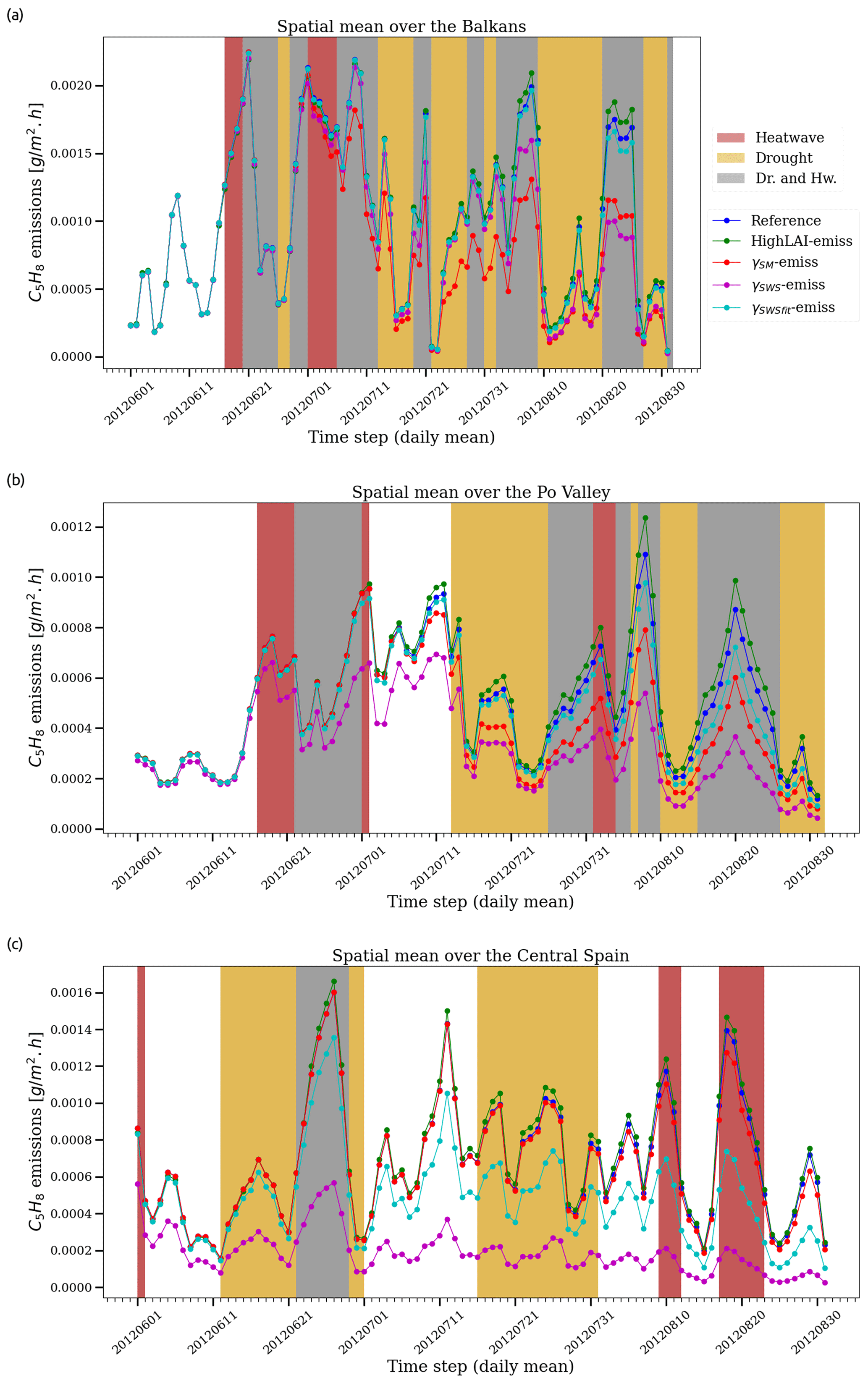
Figure 3 Daily mean C₅H₈ emissions (g m⁻² h⁻¹) during summer 2012, spatially averaged over the Balkans (a), Po Valley (b), and central Spain (c), for the different MEGAN experiments. The coloured bands highlight periods of droughts and heatwaves.

Three areas of high emissions are analysed more specifically (see the boxes in Fig. 2b), namely the Balkans, the Po Valley, and central Spain. Their temporal evolution of C₅H₈ emissions during summer 2012 for the different experiments is shown in Fig. 3. Droughts and heatwaves occurred over the three regions. Droughts do not negate the dependence on light and/or temperature, and emission peaks are driven by heatwaves with higher 2 m temperature and solar radiation (Fig. S6). However, the peak values are reduced if LAI decrease and soil dryness are accounted for. When averaged over the three regions, the biomass decrease induces a 3 % decrease in the total summer amount of C₅H₈ emitted. The soil dryness parameter induces difference of −12 % for γ_SM-emiss, −39 % for γ_SWS-emiss, and −13 % for γ_SWSfit-emiss. Based on experimental measurements over three summers (2012, 2013, and 2014) in a Mediterranean environment (Observatoire de Haute-Provence; Quercus pubescens plant species), Saunier et al. (2017) identified a 35 % emission decrease due to severe droughts. In California, Demetillo et al. (2019) measured a C₅H₈ concentration reduction of 50 % during severe droughts (2014 and 2015). These values are close to, and even above, the range of the simulated experiments. The γ_SWS-emiss experiment is considered here to be the upper limit of the reduction range of C₅H₈ emissions due to dry conditions, with SWS being included in the calculation of the emissions rate as soon as soil water stress for plant stress is below 0.5.

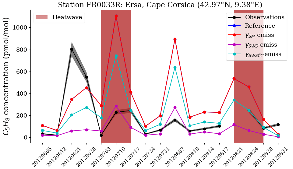
Figure 4 Observed surface C₅H₈ concentration (pmol mol⁻¹) during summer 2012 at the Ersa station (FR0033R; Cape Corsica) from the EBAS data set, compared to the different simulated experiments undertaken by the MEGAN-CHIMERE model. The shaded curve in black represents the precision range of the measurements. The reference and γ_SM-emiss experiments here have equal values. Maximum PLA_T2 m and PLA_SD are +3.2 ^∘C and −0.02 of soil dryness index, respectively.

In addition, the different simulated experiments from the MEGAN-CHIMERE model have been compared to observations of surface C₅H₈ concentrations from EBAS data set (Fig. 4). The Ersa station, having an almost complete time series for summer 2012, is kept. Based on the PLA indicator, northern Corsica was affected by two heatwaves but no drought. However, we detected soil dryness conditions close to the drought limit (mean PLA_SD of −0.09). The temporal correlation between simulated and observed C₅H₈ concentrations is similar for each experiment (R coefficient around 0.68). Averaged over the summer, the lowest mean bias with the observations is obtained with γ_SWSfit-emiss (−28 pmol mol⁻¹) and the largest one with γ_SM-emiss (−151 pmol mol⁻¹). Over July and August, the γ_SWS-emiss experiment presents the lowest mean bias (+56 pmol mol⁻¹). The reference and γ_SM-emiss experiments have equal values, as the soil wetness from WRF-Noah is above the local wilting point. However, this comparison with observations is made at a single station. It would be valuable to carry out the same exercise at several locations (including areas representative of a semi-arid environment) and over several summers.

Finally, biogenic emission models (such as MEGAN) consider a reduction in emissions in general when drought episodes occur only for isoprene (C₅H₈). However, there is a lot of uncertainty regarding how plant activity reacts to water stress. In the case of C₅H₈ species, the response to water stress could occur in two phases, i.e. a state of increasing emissions due to leaf temperature stimulation during the drought onset, followed by a state of C₅H₈ synthase limitation (Potosnak et al., 2014). For monoterpenes, the response to water stress may be different, depending on the species (Bonn et al., 2019). For instance, sabinene emissions (experimentally measured) from the European beech (Fagus sylvatica) decrease strongly with decreasing soil water availability, while trans-β-ocimene emissions (from the same plant species) remain constant.

5.1.2 O₃ dry deposition velocity

Figure 5a presents the daily mean dry deposition velocity ranging from 1.0 to 1.8 cm s⁻¹ within our areas of interest. The mean effect of biomass decrease (relative difference between the reference and the LAIdecr-dep experiment; Fig. 5b) over summer 2012 does not exceed −8 % and is lower over the forested areas (as it was prescribed in our experiment).

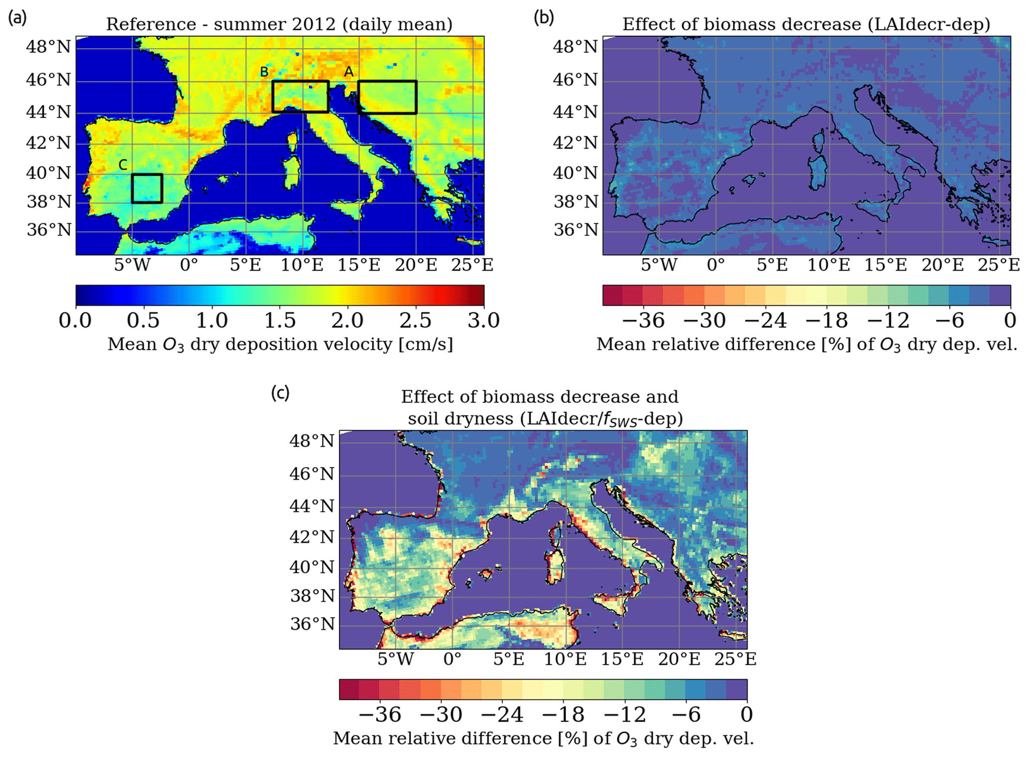
Figure 5 Summer mean (JJA) of the daily mean O₃ dry deposition velocity (cm s⁻¹) for 2012 from the reference simulation (a). The mean relative difference (%) of the O₃ dry deposition velocity is due to biomass decrease and soil dryness. The relative difference is computed between the reference and LAIdecr-dep simulation to quantify the biomass decrease effect (b) and LAIdecr-dep/f_SWS-dep to quantify the combined biomass decrease and soil dryness effect (c).

The cumulative effects of biomass decrease and soil dryness are included in the LAIdecr-dep/f_SWS-dep experiment (Fig. 5c). The soil dryness effect is much larger than that of the biomass decrease. Values range from 0 % to −35 %. Central Italy and the Iberian Peninsula are the most affected regions.

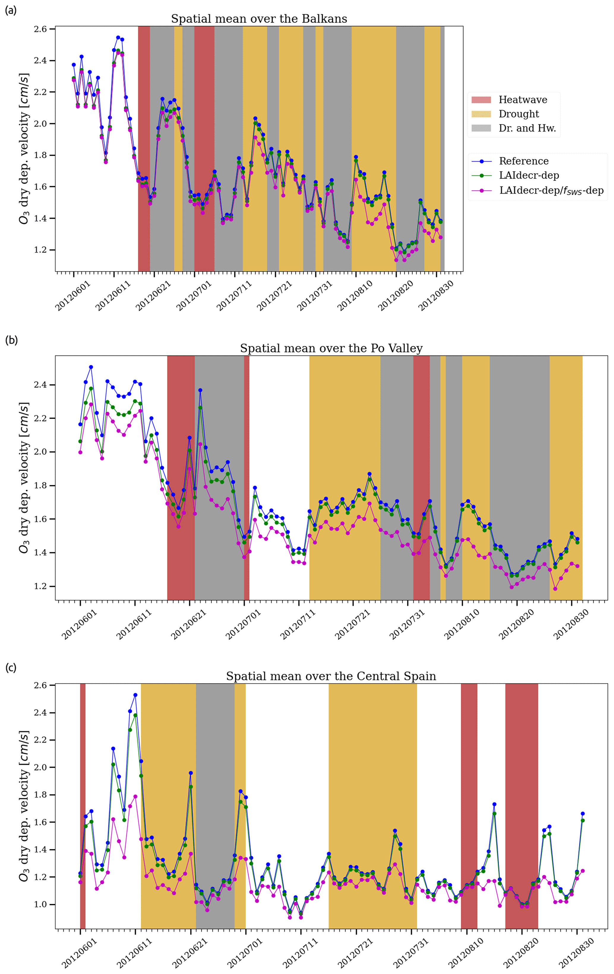
Figure 6 Daily mean O₃ dry deposition velocity (cm s⁻¹) during summer 2012, spatially averaged over the Balkans (a), Po Valley (b), and central Spain (c) for the different CHIMERE experiments.

The temporal evolution of O₃ dry deposition velocity for the three areas of interest is shown in Fig. 6. The biomass decrease effect is larger (e.g. −9 % over the Po Valley) during the first half of the summer. It is close to −1 % at the end of the summer. This is explained by the LAI decrease prescribed from mid-July in the dry deposition scheme. In addition to that, the dry deposition velocity is characterized by a decreasing trend over summer imposed by the fixed phenology factor (f_phen).

Regarding the soil dryness, its effect is almost constant during the summer (e.g. −12 % over the Po Valley). Based on measurements over central Italy, Lin et al. (2020) computed a relative difference of about −50 % between August 2004 (wet summer; ∼ 0.8 cm s⁻¹) and August 2003 (dry summer; ∼ 0.4 cm s⁻¹). However, summer 2003 was characterized by considerable heatwaves in Italy (positive PLA_T2 m), which might intensify the decrease. We emphasize that dry deposition velocity generally decreases during heatwaves (Fig. 6), as the near-surface temperature is above the optimal temperature of stomatal conductance. Both effects related to droughts and (the most intense) heatwaves lead to a reduction in O₃ deposition. The sensitivity of the dry deposition velocity to soil moisture can be considerably different from one deposition scheme to another. Using the same deposition scheme as in the present study, Anav et al. (2018) calculated an average decrease of 10 % over Europe in dry O₃ deposition.

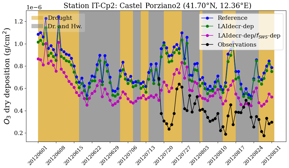
Figure 7 Observed O₃ deposition flux (g cm⁻²) during summer 2012 at the Castel Porziano station (IT-Cp2; Lazio region) from the EFDC database, compared to the different simulated experiments undertaken by the CHIMERE model. The maximum PLA_T2 m and PLA_SD are +3.88 ^∘C and +0.09 of soil dryness index, respectively.

To the best of our knowledge, there is no study yet in the scientific literature that fully assess the O₃ dry deposition of CHIMERE against observations or its sensitivity to different meteorological forcings. Therefore, we have compared our results to the measured data available for summer 2012 at the Castel Porziano station from the European Eddy Fluxes Database Cluster (Fig. 7). Based on the PLA indicator, the Lazio region was affected by a severe drought throughout the summer (mean PLA_SD of +0.05). All simulated experiments overestimate O₃ deposition compared to observations. The LAIdecr-dep/f_SWS-dep experiment has the smallest average bias (−0.19 × 10⁻⁶ g cm²) and the highest correlation (R coefficient of 0.40). Such overestimation has also been calculated for models whose gas deposition scheme is based on the description in Wesely (1989) of the big leaf parameterization (e.g. Michou et al., 2005; Huang et al., 2022). As the canopy conductance increases proportionally with the prescribed LAI (Emberson et al., 2000), this could be explained by an overestimation of the LAI that is almost 2 times larger than the mean LAI reconstructed from MODIS over this area. The importance of representing processes dynamically (as opposed to fixed parameters, especially for the non-stomatal conductance) is also highlighted in order to better simulate the diurnal deposition cycle and the daily average values (Huang et al., 2022).

Finally, identifying soil dryness as a major driver of interannual variability in O₃ deposition velocity, Lin et al. (2019) emphasize that the error in modelling the deposition may considerably rely on the ability of the models to accurately simulate the precipitation distribution. They assessed the sensitivity of their deposition velocity scheme (Geophysical Fluid Dynamics Laboratory, LM3.0/LM4.0) to two different meteorological forcings and found a factor of 2 over northern Europe.

5.1.3 O₃ surface concentration

Figure 8a maps the mean surface O₃ concentration simulated by CHIMERE (reference experiment) over summer 2012. High concentrations (between 100 and 110 µg m⁻³) are located in the eastern part of the study area (e.g. the Balkans and Italy). The spatial distribution of the mean surface O₃ shows similar patterns to the distribution of PLA_T2 m (Fig. S2), highlighting the critical role of the temperature. Surface O₃ remains high above the sea due to transport and the absence of deposition in the canopy (e.g. 120 µg m⁻³ over the Adriatic sea). The contribution of BVOC emissions on surface O₃ is also presented (Fig. 8b). BVOC emissions are known to be significant precursors of O₃ production in the Mediterranean region. It varies between 4 % (e.g. Iberian Peninsula) and 22 % (e.g. northern Italy) in our study, and that is included in the range of values reported in the scientific literature (e.g. Mertens et al., 2020). Finally, our areas of interest are located in rural regions mostly characterized by a low-NO_x regime (Fig. S7).

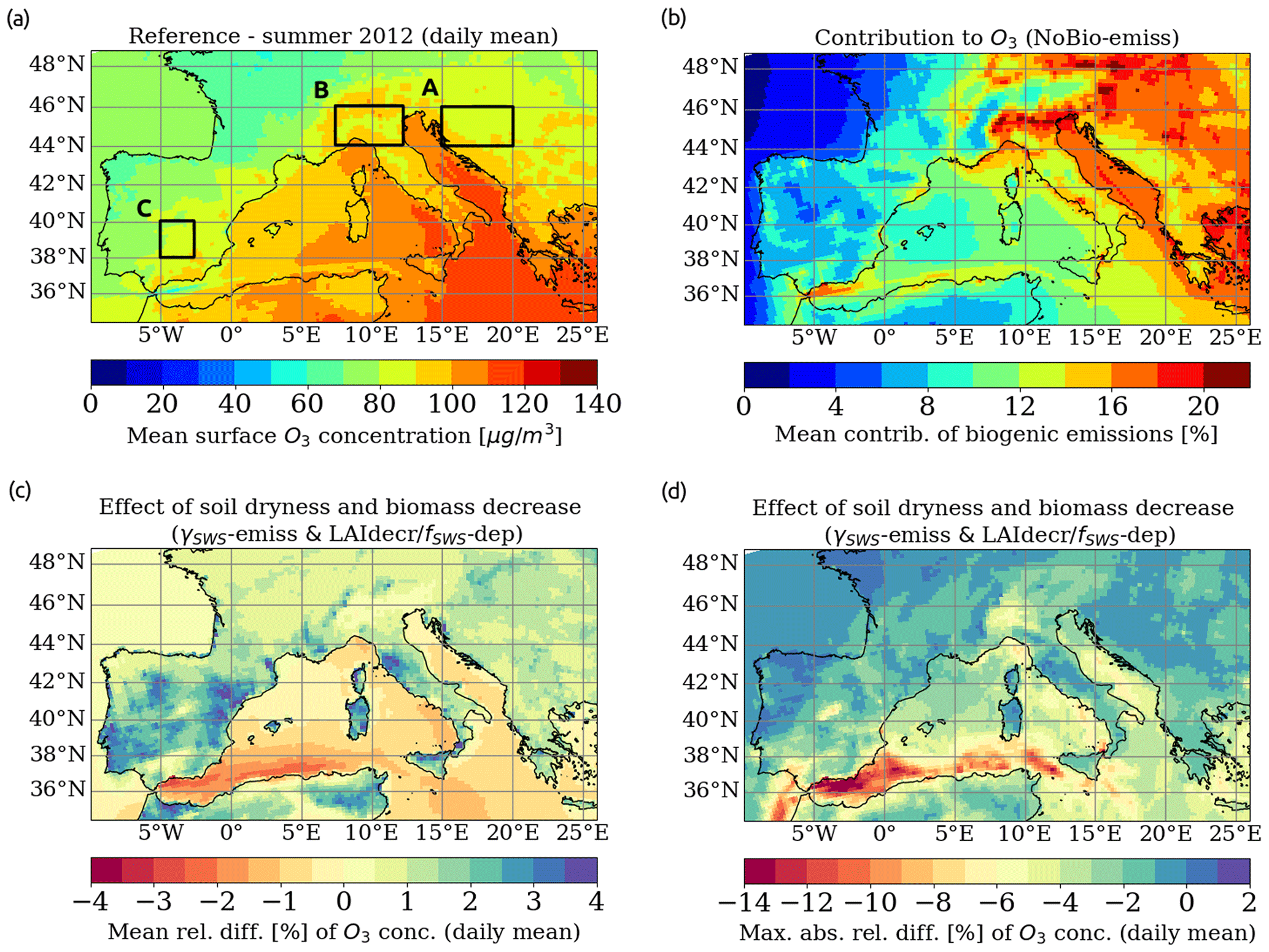
Figure 8 Summer mean (JJA) of daily mean O₃ surface concentration (µg m⁻³) for 2012 from the reference simulation (a). The mean contribution of biogenic emissions to O₃ surface concentration is based on the NoBio-emiss experiment (b). The mean (c) and maximum absolute (d) relative difference (%) of the O₃ surface concentration due to the biomass decrease and soil dryness. The relative difference is computed between the reference and γ_SWS-emiss and LAIdecr-dep/f_SWS-dep simulation from CHIMERE.

A simulation including drought effects on both C₅H₈ emissions and O₃ dry deposition has been conducted with MEGAN-CHIMERE (γ_SWS-emiss and LAIdecr/f_SWS-dep experiment). The resulting effect on surface O₃ is shown in Fig. 8. On average, during the summer (Fig. 8c), the O₃ concentration is slightly higher over the continent (between +0.5 % and +3.0 %) due to the decrease in O₃ deposition as a dominant effect, while it is slightly lower (between −1 % and −1.5 %) over the sea and ocean due to the lower transport of O₃ precursors, compared to the reference experiment. However, the O₃ increase over the Iberian Peninsula may be overestimated, as the LAI reduction we applied to the whole domain (e.g. −20 % for grass PFTs) is larger compared to the variation in MODIS LAI in this specific region (Fig. S3).

Drought effects on surface O₃ induced by the C₅H₈ emission reduction is not constant. It is largest during combined heatwaves (i.e. when the biogenic contribution is high). As a result, drought effects on C₅H₈ emissions can be dominant (compared to the effects on O₃ deposition) during simultaneous droughts and heatwaves, inducing a decrease in O₃ peaks by a few micrograms per cubic metre (µg m⁻³) over both the continent and sea/ocean. The maximum absolute relative difference (Fig. 8d) reaches −5 % over the Po Valley and −14 % along the Strait of Gibraltar. O₃ formation over the latter is favoured by large NO_x shipping emissions.

Conducting a similar modelling experiment based on the γ_SM from MEGANv3, Jiang et al. (2018) simulated a maximum absolute relative difference in surface O₃ of about −4 % in August 2010. O₃ reduction (−10 % on average) due to severe droughts was also measured in California over the period 2002–2015 (Demetillo et al., 2019). This was identified as being related to a steep decrease in C₅H₈ concentrations.

Figure 9 Daily mean O₃ surface concentration (µg m⁻³) during summer 2012 that is spatially averaged over the Po Valley from the EEA observations and the different CHIMERE experiments.

For each area of interest, the temporal evolution of surface O₃ based on the different CHIMERE experiments and the EEA observations (AQ e-Reporting) is presented (Fig. 9 for the Po Valley and Fig. S8 in the Supplement for the Balkans and central Spain). Since the resulting effects of biomass decrease and soil dryness on surface O₃ are less than the bias between model and observations in our study (see Sect. 4), no simulation can be designated with certainty as the best fit.

5.2 Statistical variation during droughts and heatwaves

In this result section, a statistical analysis is performed using CHIMERE simulations and several observational data sets. The all-emiss-dep experiment has been chosen for simulating summers 2012–2014 because it includes drought and heatwave effects in the most comprehensive way. Moreover, the C₅H₈ emission approach γ_SWSfit-emiss has shown a good performance compared to observations (Fig. 4), remaining rather conservative and not being in the upper limit of the C₅H₈ reduction range.

Clusters of droughts and heatwaves (isolated or combined) are constructed based on the PLA_T2 m and PLA_SD indicators, allowing the analysis of the statistical variation in simulated C₅H₈ emissions, O₃ stomatal conductance, and O₃ surface concentration for the summers of 2012–2014. We performed the same analysis on observations of HCHO total column for the summers of 2005–2016 and O₃ the summers of 2000–2016. Using those indicators, the following conditions were defined and grouped into the following clusters: (1) heatwaves, (2) droughts, (3) heatwaves or droughts, (4) heatwaves and droughts, (5) heatwaves and not droughts, and (6) droughts and not heatwaves. Normal conditions are defined as (7) no drought and no heatwave.

5.2.1 C₅H₈ emissions

Figure 10 shows the distribution of C₅H₈ emission rates over the southwestern Mediterranean for clusters of extreme weather events. On average, the daily maximum C₅H₈ emission is significantly higher (t test; p<0.01) during isolated and combined heatwaves than normal conditions (no heatwave nor drought), with a mean value of $\mathrm{0.16}\times {\mathrm{10}}^{-\mathrm{2}}$ against $\mathrm{0.12}\times {\mathrm{10}}^{-\mathrm{2}}$ g m⁻² h⁻¹. However, emissions during droughts have the same mean value as in normal conditions. During isolated droughts (cluster drought and not heatwave), the mean daily maximum C₅H₈ emission rate is lower than normal conditions ($-\mathrm{0.02}\times {\mathrm{10}}^{-\mathrm{2}}$ g m⁻² h⁻¹; non-significant difference). These results are in general agreement with the observed HCHO total column by satellite instrument, used as proxy for BVOC emissions variation (see Sect. 5.2.2). Weather conditions are considerably different between the droughts combined with heatwaves and those which are not (Fig. S9). The combined (respectively, isolated) droughts are characterized by a 2 m temperature of 23.9 ^∘C (respectively, 22.6 ^∘C), a shortwave radiation of 342.2 W m⁻² (respectively, 296.0 W m⁻²), and a cloud cover of 1.8 % (respectively, 3.1 %). Those weather variables are used for the computation of the activity factors γ_P and γ_T, thus directly affecting emissions. During isolated droughts, γ_LAI (0.48) and γ_SWS (0.76) are smaller than for normal conditions (0.51 and 0.89, respectively, with a significant difference for both). Nevertheless, this negative signal is not large enough for a significant variation in the emission rates (compared to normal conditions). Gathering worldwide data from experimental measurements of biogenic emissions under different climate drivers, the scientific review presented by Feng et al. (2019, based on 74 articles) estimated a +53 % emission change in C₅H₈ during warm conditions and a −15 % change during dry conditions. Those variations are close to what we simulated (+35 % and −13 %, respectively).

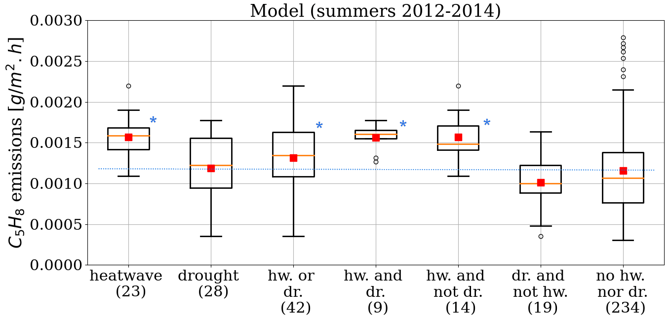
Figure 10 Daily maximum C₅H₈ emission rate (g m⁻² h⁻¹) simulated by the MEGAN model (γ_SWSfit-emiss experiment) over southwestern Europe, clustered by identified extreme weather events (PLA_T2 m and PLA_SD indicators from RegIPSL). The number of days is indicated in parentheses. The analysed period is June–August in 2012, 2013 ,and 2014, covering a total of 276 d. The red squares show the mean of the distribution, and the black circles are the outliers. The blue dotted line indicates the mean value of the normal conditions (no hw. nor dr. cluster), and the blue stars show if the mean value of the considered cluster is significantly different (t test; at least p<0.1) from the normal conditions. The box covers the interquartile range (IQR) between Q1 (25th percentile) and Q3 (75th percentile). The lower whisker is limited to a statistical minimum (Q1 − 1.5 × IQR) and the upper one to a statistical maximum (Q3 + 1.5 × IQR).

5.2.2 HCHO total column

HCHO is a product of the oxidation of VOCs. Based on the reference and NoBio-emiss CHIMERE simulations, we computed that biogenic emissions contribute between 60 % and 80 % of the HCHO concentration over southwestern Europe. Variations in the HCHO concentration may therefore be used as indicator of BVOC emission variations during droughts and heatwaves. This allows us to use satellite observations of HCHO, which is particularly interesting due to the lack of in situ data. Observations of the HCHO total column from the OMI instrument are used.

Table 3 Variation in HCHO total atmospheric column (molec. cm⁻²) (ΔHCHO) due to heatwaves, droughts, and isolated droughts in comparison to normal conditions (norm. cdt.; no heatwaves nor droughts) for the summers (JJA) between 2005–2016 (measurements at 13:00 LT, local time). Summer 2012 is compared with CHIMERE simulations. Results are computed for each pixel and averaged over the following areas of interest: the Balkans, central Italy, and central Spain. The asterisks mean that the difference with normal conditions is statistically significant (t test; p<0.1).

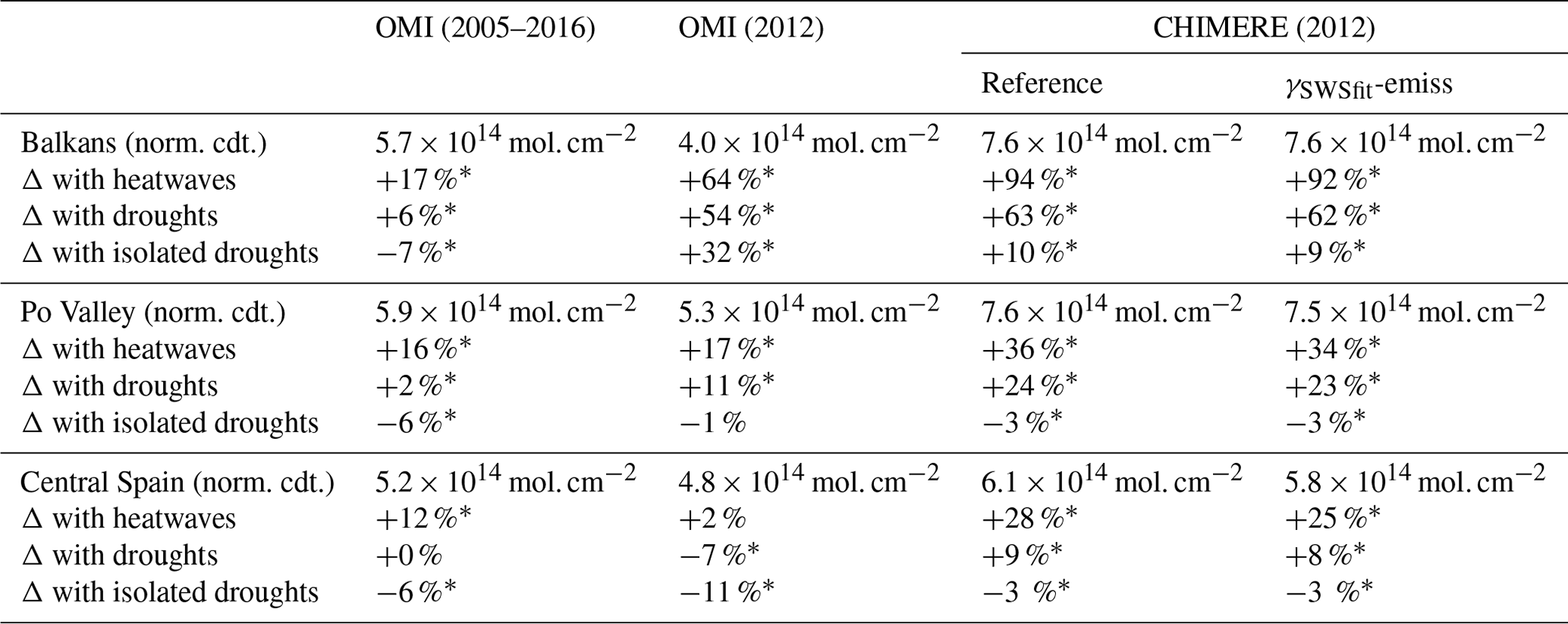
Table 3 presents the average difference in HCHO (ΔHCHO) during extreme events compared to normal conditions (no heatwave nor drought), based on the OMHCHOd product. Over the summers of 2005 to 2016, HCHO is significantly higher during heatwaves for the Balkans, Po Valley, and central Spain (+15 % on average). ΔHCHO is also positive during droughts but to a lesser extent (+3 % on average, non-significant for central Spain only). However, isolated droughts induce a significant decrease for the Balkans (−7 %), Po Valley (−6 %), and central Spain (−6 %). Those results are consistent with the variation in C₅H₈ emissions simulated by MEGAN when a soil moisture parameter is considered (see Sect. 5.2.1). P. Wang et al. (2021) also report a significant HCHO column decrease (up to −30 %) induced by a prolonged drought in a forested area in China.

The observed and simulated HCHO total columns have been compared for the γ_SWSfit-emiss experiment over summer 2012. The time series showing the HCHO evolution for the three areas of interest are shown in the Supplement (Fig. S11). Simulated HCHO columns are generally higher than those from the observations, especially for the Balkans. As mentioned in Sect. 2.2, uncertainty in the observations is large (between 30 % and 100 %), with a large spatial variability (about a factor of 2 larger than in CHIMERE). HCHO products from OMI also present high uncertainty and, in particular, a systematic low mean bias (20 %–51 %; Zhu et al., 2016).

HCHO differences could be due to incorrect specifications of land cover and, thus, of the EF of C₅H₈ (e.g. Curci et al., 2010). Temperate tree PFTs are characterized by high C₅H₈ emission rates (respectively, 10 000 and 600 µg m⁻² h⁻¹ for broadleaf and needleleaf types) compared to grassland (800 µg m⁻² h⁻¹) or cropland (1 µg m⁻² h⁻¹; Guenther et al., 2012). After the aggregation of the USGS land cover classes, the vegetation type assumed in CHIMERE in the Balkans, for instance, is 57 % forest cover, 9 % grassland, and 33 % cropland. Using the MODIS MCD12 product (Friedl et al., 2010), we find a different distribution, with 30 % forest cover, 25 % grassland, and 31 % cropland (Fig. S10). The choice and the temporal evolution of the land cover database are crucial for the calculation of C₅H₈ emissions (Chen et al., 2018). Despite the use of satellite data for land cover, significant uncertainties remain in the calculation of C₅H₈ emissions due to the classification of vegetation types and species (Opacka et al., 2021).

The comparison of the HCHO total column variations for CHIMERE and OMI during droughts and heatwaves relies on a limited number of cases. It is therefore difficult to support conclusions with a sufficient level of certainty. Nevertheless, results suggest that CHIMERE simulations are more sensitive to temperature than the OMHCHOd OMI observations (+52 % and +28 % during heatwaves, respectively, averaged over the three areas of interest). Since the summer 2012 was affected by long agricultural droughts, the inclusion of a soil dryness parameter in CHIMERE (γ_SWSfit-emiss experiment) reduces the simulated HCHO peaks (Fig. S11). However, the mean simulated ΔHCHO during heatwaves and droughts is similar in the γ_SWSfit-emiss and reference experiments (decrease of −2 % and −1 %, respectively). The temporal correlation does not vary significantly either (e.g. R coefficient around 0.5 for the Balkans).

Finally, the observed variations in total HCHO over the summers of 2005–2006 and the three areas considered here were also computed with OMI-BIRA retrieval. During heatwaves, both show a significant increase, i.e. +31 % for OMI-BIRA (and +15 % for OMHCHOd). The increase is lowers by +13 % (and +3 %) during drought. The variation becomes slightly negative during isolated droughts, i.e. −2 % (and −6 %). This comparison not only highlights the uncertainty in the satellite observations but also that the general behaviour is consistent in both retrievals and similar to what was obtained for 2012 using CHIMERE.

5.2.3 O₃ stomatal conductance

Surface weather conditions are critical for the stomatal conductance and therefore influence the dry deposition velocity. Figure 11 shows the maximum daily stomatal conductance of O₃ (LAIdecr/f_SWS-dep CHIMERE experiment) clustered by simulated extreme weather events and averaged over the western Mediterranean. The same analysis has been performed on the dry deposition velocity, and the signals induced by extreme weather events are similar.

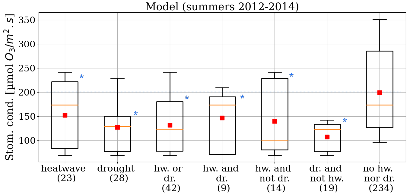
Figure 11 Same as Fig. 10 with the simulated O₃ stomatal conductance (µmol O₃ m⁻² s⁻¹) by the CHIMERE model (LAIdecr/f_SWS-dep experiment).

Droughts and heatwaves (isolated or combined) induce a significant decrease in the O₃ stomatal conductance, quantified at −25 % for heatwaves and −35 % for droughts, compared to normal conditions. The activity factors mainly affected by droughts and heatwaves are f_temp, f_VPD, and f_SWS.

The variation in f_temp during heatwaves depends on the magnitude of the events and also on their location, since the percentile of the PLA indicator is defined for each grid cell. Over the Po Valley and Balkans, for instance, most heatwaves are characterized by temperatures close to optimal values of stomatal conductance that are fixed around 24 ^∘C (Fig. S6). However, for those occurring in central Spain (between 30 and 32 ^∘C), f_temp decreases by 7 % compared to normal conditions. The temperature limit before complete stomatal closure is set at 40 ^∘C. Therefore, exceptional heatwaves occurring in southern Spain, for instance, could quickly lead to an accumulation of O₃ at the surface. f_VPD that depends both on temperature and relative humidity significantly decreases during droughts and heatwaves (e.g. −6 % averaged over southwestern Europe). Finally, f_SWS is the factor dominating the signal of variation in stomatal conductance. At the scale of southwestern Europe, this factor is the lowest during isolated droughts, with a mean decrease of −35 %.

5.2.4 O₃ surface concentration

Figure 12 shows the distribution of the observed (summers 2000–2016 and 2012–2014) and simulated (summers 2012–2014) daily maximum surface O₃ concentrations over southwestern Europe for each cluster of extreme events. Observed O₃ (Fig. 12a) is significantly (t test; p<0.01) higher during heatwaves (+18 µg m⁻³) and droughts (+9 µg m⁻³) than during normal conditions. Considering all droughts over the United States of America, Wang et al. (2017) also computed a mean increase in surface O₃ (+17 % compared to the average). During isolated droughts in our study area, the daily maximum O₃ is larger (+4 µg m⁻³), but the difference is non-significant.

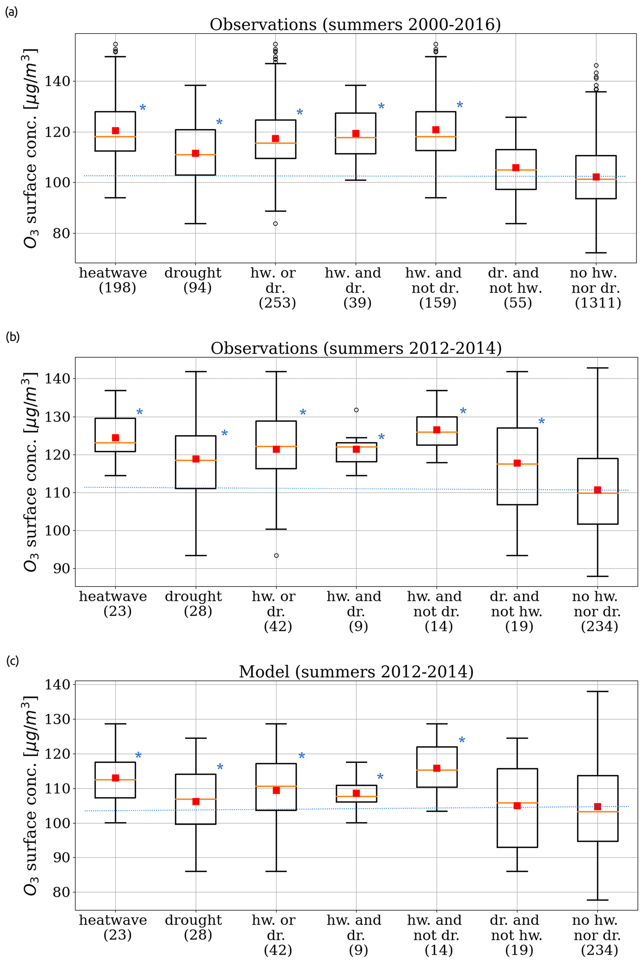
Figure 12 Same as Fig. 10 with the observed surface O₃ concentration (µg m⁻³) over the summers of 2000–2016 (a) and 2012–2014 (b) and with the simulated surface O₃ (all-emiss-dep experiment) over the summers of 2012–2014 (c).

The distribution of the simulated surface O₃ (all-emiss-dep experiment) by extreme events over the period 2012–2014 (Fig. 12c) presents similar signals, but of lower magnitude, with +9 µg m⁻³ during heatwaves, +3 µg m⁻³ during droughts, and a non-significant difference during isolated droughts compared to normal conditions. Based on the results discussed above, the difference between the heatwave and isolated drought cluster could be explained by the different conditions of biogenic emissions, dry deposition, temperature, and light. However, observations over the same period (Fig. 12b) present a significant increase in the daily maximum O₃ during isolated droughts (+9 µg m⁻³), unlike what we simulated. The C₅H₈ emission reduction effect during such an extreme event could be counterbalanced to a larger extent by the O₃ dry deposition decrease. It could also be explained by an underestimated impact of the enhanced photochemistry in the simulations, as we simulated favourable weather conditions during both combined and isolated droughts.

In summary, the variation in canopy–troposphere interactions (simulated by the MEGAN and CHIMERE models) during droughts and heatwaves is characterized by a consistent signal with respect to O₃ observations (except for the isolated droughts over summers 2012–2014). Meteorological conditions are critical for the O₃ budget, especially during summer droughts and heatwaves. In addition to uncertainties in the modelling of precursor emissions and O₃ deposition (as mentioned above), differences between observations and simulations may also rely on meteorological uncertainties, such as the diurnal temperature cycle (see Sect. 4) and the planetary boundary layer height (PBLH). The nighttime representation of the PBLH is often misrepresented in the WRF model (e.g. Chu et al., 2019).

5.3 Threshold level exceedance of O₃

In the European Union, the air quality standard for O₃ exposure is set at a daily maximum concentration of 120 µg m⁻³ (8 h average; EEA, 2020). Figure 13 shows the number of days above this threshold based on the AQ e-Reporting observations and the CHIMERE all-emiss-dep simulations for the summers of 2012, 2013, and 2014. The summers of 2012 and 2013 present a large number of days exceeding the standard concentration. Even if exceedances occur in similar regions for observations and simulations, the number of days is generally larger in the observations. This is due to the overall underestimated daily maximum in CHIMERE compared to observations (see Sect. 4). For example, in the Po Valley that is the most affected region in southwestern Europe, around 60 exceeding days were observed and 50 d were simulated over summer 2012. This region is known for its highly polluted air (O₃ and its precursors) due to high anthropogenic emissions and unfavourable topographic and meteorological conditions for pollutants dispersion (e.g. Bigi et al., 2012). Other regions affected by O₃ peaks can be highlighted, southeastern France, central Spain, and central Italy, for the summers of both 2012 and 2013.

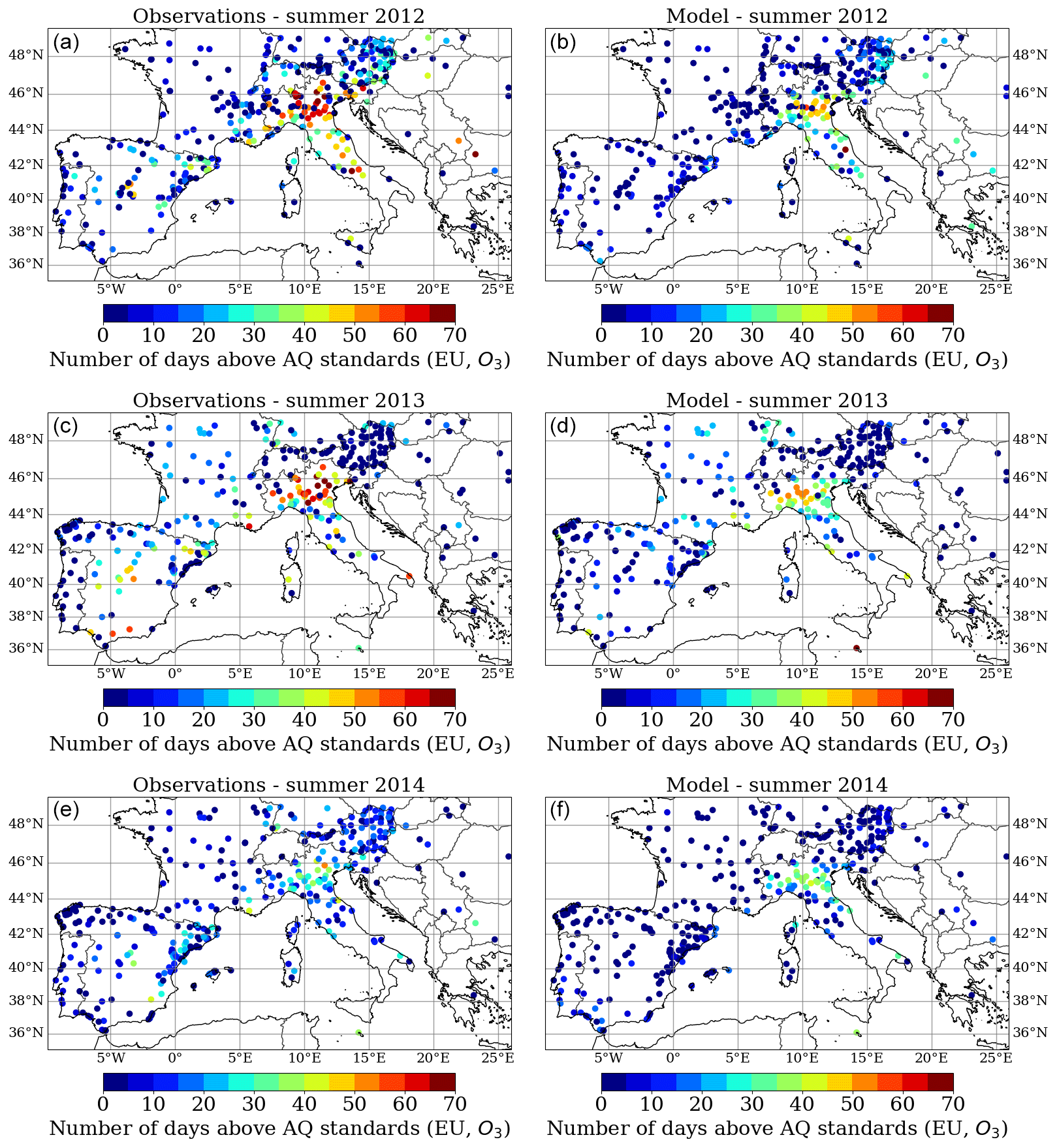
Figure 13 Number of days above the air quality threshold value from the European Union for surface O₃ (maximum daily 8 h mean of 120 µg m⁻³) over the summers of 2012, 2013, and 2014 (JJA; 92 d in total). EEA observations (left column) are compared to CHIMERE (all-emiss-dep) simulations (right column).

Table 4 Average percentage of stations with at least 1 exceedance day (first row) regarding EU standard during summer (JJA). Considering only those stations, the second row shows the average number of exceeding days (exc. days) per station and the lower rows the average distribution of days above the EU standard as a function of extreme weather events. The mean exceedance concentration is indicated in parenthesis.

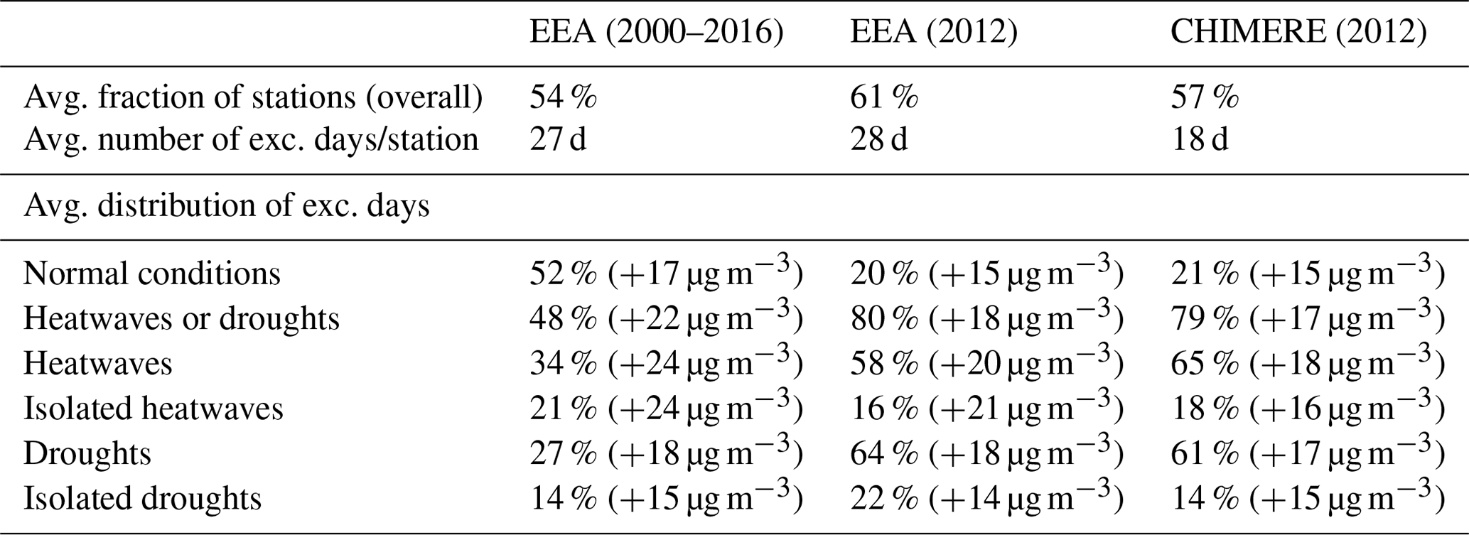
Table 4 presents the distribution characteristics of stations with at least 1 d above the EU standard during summer period. On average, over 2000–2016, that concerns 54 % of EEA stations over the western Mediterranean. The average number of exceedance days per station is 27 d (almost a third of the summer period). Summer 2012 is above the 2000–2016 average, with 61 % of stations affected and 28 d on average per station. For the same year, co-located values from CHIMERE simulations (all-emiss-dep experiment) are lower, i.e. 57 % of stations and 18 d on average.

Over all the summers between 2000 and 2016, 34 % of the exceeding days occurred during heatwaves (with a mean exceeding value of 24 µg m⁻³) and 27 % during droughts (+18 µg m⁻³). The number of days decreases by 13 % if we consider only the isolated droughts (14 %; +15 µg m⁻³). Summer 2012 was affected by exceptional droughts and heatwaves, resulting in high O₃ pollution. Around 80 % of the days above the EU threshold occurred during heatwaves or droughts for both observations and simulations.

6 Discussion and conclusions

The analyses presented in this study were organized around two main objectives. The first one was to assess the sensitivity of biogenic emissions, O₃ dry deposition, and surface O₃ to the biomass decrease and soil dryness effect in a CTM model. The extremely dry summer of 2012 was chosen, and simulations were performed using the MEGAN v2.1 and CHIMERE v2020r1 model. We showed that the soil dryness parameter is critical during drought events, decreasing the C₅H₈ emissions and O₃ dry deposition velocity considerably. This effect has a larger impact than the biomass decrease. However, the resulting effect on surface O₃ remains limited.

In addition to the soil moisture activity factor used in MEGAN v2.1 that is mainly based on the wilting point (γ_SM), we proposed an innovative activity factor based on a soil water stress function (γ_SWS) simulated by the land surface and vegetation model ORCHIDEE. The latter induces a larger reduction in C₅H₈ emissions with more homogeneous patterns that follow the drought indicator. Furthermore, we adjusted this factor with a function fitted (γ_SWSfit) from experimental measurements in Bonn et al. (2019). By comparing the simulated surface concentration of C₅H₈ with observations at the Ersa measurement site (Corsica), γ_SWSfit showed promising results. However, such an evaluation should be carried out over several sites and several years in order to determine the added value of this approach with more certainty.

The second objective of this study was to quantify the variation in surface O₃ over southwestern Europe during agricultural droughts when combined, or not, with heatwaves. Those extreme weather events were identified based on the RegIPSL model using the PLA indicator. During the 2000–2016 period, 59 % of summer drought days were not accompanied by heatwaves (isolated droughts). For the summers of 2012–2014, analysed more specifically in this study, the 2 m temperature is on average 5.5 % lower during isolated droughts compared to all droughts, the shortwave radiation is 13.5 % lower, and the cloud fraction is 42 % higher. As a result, not only surface O₃ but also BVOC emissions and O₃ dry deposition velocity are substantially different if the drought considered is accompanied by a heatwave or not.

Based on a cluster approach using the PLA indicator, we showed that observed surface O₃ (summers of 2000–2016) is larger by +18 µg m⁻³ in the daily maximum during heatwaves and by +9 µg m⁻³ during droughts, compared to normal conditions. Despite a difference of several micrograms per cubic metre (µg m⁻³), CHIMERE correctly simulates the variations in O₃ concentration between the clusters of extreme events. The overall increase in surface O₃ during both heatwaves and droughts would be explained by the O₃ precursor emission enhancement, O₃ dry deposition decrease, and favourable weather conditions, so that all of these mechanisms lead to an accumulation of O₃. However, we simulated a decrease in C₅H₈ emissions during isolated droughts, resulting in a non-significant difference in surface O₃ compared to normal conditions (from both observations and simulations). Despite a significant bias between the HCHO total columns simulated by CHIMERE and observed by OMI, the satellite data confirm an average increase in HCHO (+3 % to +13 %, depending of the product considered) over our three regions of interest for all droughts and a decrease (−2 % to −6 %) for isolated droughts.

Finally, almost half of the summer days (2000–2016 period) exceeding the EU standard of O₃ for air quality in southwestern Europe occurred during droughts or heatwaves. However, this percentage can increase (up to 80 %) for exceptionally dry and hot summers, as in 2012. Only 14 % of the exceedance days occurred during isolated droughts.

The implementation of the dynamical effects of droughts in the MEGAN-CHIMERE model contributes to a better representation of biosphere–atmosphere interactions. However, comparisons between simulated and observed surface O₃ still show large discrepancies. Important uncertainties appear to be related to BVOC emissions (especially due to the land cover classification), to NO_x concentrations, for which CHIMERE presents limited performance scores of validation, to O₃ deposition, and, finally, to meteorological conditions (e.g. temperature and PBLH). For instance, the simulated daily maximum temperature that is underestimated in the northern Mediterranean, compared to observations (see Sect. 4), may induced a decrease in O₃ precursors, especially as the emission–temperature relationship of BVOCs is exponential, with an optimal temperature for C₅H₈ species (Guenther et al., 1993). Such uncertainties need to be addressed to improve the simulation of O₃ during the summer, especially over southwestern Europe.

In addition, the critical role of soil NO emissions in O₃ production is increasingly studied (e.g. Romer et al., 2018), especially in rural areas (e.g. Sha et al., 2021). As hydroclimatic conditions are critical for soil NO emissions, the O₃ budget during droughts and heatwaves is likely to be significantly influenced by soil NO emissions. In this study, the dependence on soil dryness for NO emissions is not included. Emission pulses can occur when rain follows a drought, and emission factors are higher with dry soil than with wet soil (Steinkamp and Lawrence, 2011; Weng et al., 2020).

Some recent knowledge on fundamental processes that allow a better representation of surface–atmosphere interactions during extreme weather events is not yet integrated by much, if not all, of the modelling community. Among the many examples is the increased emission of monoterpenes and sesquiterpenes during the development of drought (e.g. Bonn et al., 2019; Peron et al., 2021) or the in-canopy chemistry that is ignored or approximated by the big leaf model approach (e.g. Clifton et al., 2020a). Several studies show that non-stomatal conductance in the Mediterranean counts as much as stomatal conductance in the O₃ sink budget (e.g. Gerosa et al., 2009; Sun et al., 2022). Moreover, non-stomatal conductance also seems to be significantly affected during droughts and heatwaves. In contrast to stomatal conductance, droughts and heatwaves should have opposite effects, i.e. an increase in non-stomatal conductance during heatwaves and a decrease during droughts (Wong et al., 2022). However, such changes are not taken into account in the EMEP deposition scheme implemented in CHIMERE. There is a real need for a better representation of stomatal conductance in deposition schemes.

In conclusion, we provide in this paper a detailed analysis of the drought and heatwave effects on modelled biosphere–troposphere interactions controlling surface O₃ concentration, and our findings are supported by several observational data sets. Heatwaves, and droughts to a lesser extent, induce a significant increase in the surface O₃. Soil dryness and biomass decrease, as specific effects of droughts, are critical for the variation in C₅H₈ emissions and O₃ dry deposition over southwestern Europe. We emphasize the need for a more dynamical representation of interactions between vegetation, meteorology, and atmospheric chemistry in models in order to improve the simulation of summer O₃.