Morphological features and water solubility of iron in aged fine aerosol particles over the Indian Ocean

Atmospheric transport of iron (Fe) in fine anthropogenic aerosol particles is an important route of soluble Fe supply from continental areas to remote oceans. To elucidate Fe properties of aerosol particles over remote oceans, we collected atmospheric aerosol particles over the Indian Ocean during the RV Hakuho Maru KH-18-6 cruise. After aerosol particles were collected using a cascade impactor, particles of 0.3–0.9 µm aerodynamic diameter on the sample stage were analyzed using transmission electron microscopy (TEM) with an energy-dispersive X-ray spectrometry analyzer. The particle shape and composition indicated that most particles collected north of the Equator were composed mainly of ammonium sulfate. Regarding the particle number fraction, 0.6 %–3.0 % of particles contained Fe, which mostly co-existed with sulfate. Of those particles, 26 % of Fe occurred as metal spheres, often co-existing with Al or Si, regarded as fly ash; 14 % as mineral dust; and 7 % as iron oxide aggregates. Water dialysis analyses of TEM samples indicated Fe in spherical fly ash as being almost entirely insoluble and Fe in other morphological-type particles as being partly soluble (65 % Fe mass on average). Global model simulations mostly reproduced observed Fe mass concentrations in particulate matter with a diameter of less than 2.5 µm (PM_2.5) collected using a high-volume air sampler, including their north–south contrast during the cruise. In contrast, a marked difference was found between the simulated mass fractions of Fe mineral sources and the observed Fe types. For instance, the model underestimated anthropogenic aluminosilicate (illite and kaolinite) Fe contained in matter such as fly ash from coal combustion. Our observations revealed multiple shapes and compositions of Fe minerals in particles over remote ocean areas and further suggested that their solubilities after aging processes differ depending on their morphological and mineral types. Proper consideration of such Fe types at their sources is necessary for accurately estimating atmospheric Fe effects on marine biological activity.

1 Introduction

Iron (Fe) is recognized as an essential micronutrient for ocean primary productivity. The addition of water-soluble Fe into remote oceans, designated as high-nutrient and low-chlorophyll regions, stimulates phytoplankton blooms. Iron can thereby change the marine environment, alter biological diversity, and influence the global carbon cycle (Martin and Fitzwater, 1988; de Baar et al., 1995; Harrison et al., 1999; Jickells et al., 2005; Tsuda et al., 2003, 2007; Iwamoto et al., 2009). Transport and deposition of atmospheric aerosol particles constitute an important route supplying Fe to remote ocean areas (e.g., Uematsu et al., 1983; Jickells and Moore, 2015; Ito et al., 2019). Chief sources of soluble Fe in the atmosphere are Fe-containing mineral dust and Fe emitted from anthropogenic combustion and biomass burning (combustion Fe) (e.g., Guieu et al., 2005; Mahowald et al., 2009). Mineral dust is borne aloft mainly as coarse particles by dust storms occurring in arid and semi-arid continental areas (Zhang et al., 2003; Zhao et al., 2010; Mahowald et al., 2014). In contrast, combustion Fe is emitted as both fine and coarse particles through evaporation of metals at higher temperatures in thermal sources and condensation processes that occur with diffusion and cooling (Markowski and Filby, 1985; Liu et al., 2018; Ohata et al., 2018). Although many earlier studies have implicated mineral dust as an important source of soluble Fe transferred to oceans (e.g., Uematsu et al., 1983; Mahowald et al., 2005; Iwamoto et al., 2011), anthropogenic Fe has also attracted increasing attention recently as a source supplying water-soluble Fe, steadily and efficiently, by long-range transport (Chuang et al., 2005; Sedwick et al., 2007; Luo et al., 2008; Takahashi et al., 2013; Ito, 2015; Matsui et al., 2018b).

Recent sophisticated global aerosol modeling studies have evaluated global climatic effects of anthropogenic Fe (e.g., Scanza et al., 2018; Matsui et al., 2018b; Rathod et al., 2020). Matsui et al. (2018b) demonstrated that the atmospheric burden of anthropogenic combustion Fe is 8 times greater than earlier estimates had suggested. Simulations conducted using a soluble Fe mechanism designed for Earth system models by Scanza et al. (2018) have incorporated consideration of changes in Fe solubility that occur with atmospheric processes that affect Fe in dust and combustion aerosols. Those simulations indicated that, in many remote ocean regions, sources of Fe from combustion and dust aerosols are equally important. Moreover, Rathod et al. (2020) released a revised emission inventory of anthropogenic combustion Fe that was produced using a technology-based methodology. However, the accuracy of current model-based estimates remains unclear because of the lack of information related to the mineral composition, morphological structure, and solubility of actual Fe-containing particles in the atmosphere, especially in remote ocean areas.

Actually, Fe is emitted as aerosol particles having various morphologies, with their mineralogy and size distributions according to their sources (e.g., Jeong et al., 2014; Ingal et al., 2018; Umo et al., 2019; Ohata et al., 2018; Rathod et al., 2020). In addition, changes in Fe solubility with particle aging processes depend on many factors such as Fe mineralogy and size, atmospheric and meteorological conditions, and particle acidity (Wiederhold et al., 2006; Journet et al., 2008; Cwiertny et al., 2008; Shi et al., 2009, 2015; Ito and Feng, 2010; Li et al., 2017; Sakata et al., 2022). This earlier knowledge about relations between solubility, Fe mineral species, and aging processes has usually been based on bulk sample measurements, laboratory experiment findings, and simulation results. To evaluate model results, Fe mass concentrations and solubilities measured during numerous observation studies and chemical analyses of bulk samples have been used (Mahowald et al., 2009; Wang et al., 2015; Myriokefalitakis et al., 2018; Rathod et al., 2020). Nevertheless, data of bulk samples alone do not provide adequate information about the source, mineralogy, atmospheric aging, or solubility of individual Fe-containing particles. Enhancing our understanding of the roles and effects of atmospheric Fe on marine environments necessitates the elucidation of details of atmospheric Fe properties in remote areas far from the Fe sources.

Compared with major aerosol components such as sea salt and sulfates, Fe is a trace element that accounts for only a small fraction among components, especially in remote, weakly affected areas that are from the source (Seinfeld and Pandis, 2006). This relative scarcity of Fe makes it difficult to find and investigate Fe-containing particles in aerosol samples. Nevertheless, some observations made in leeward areas of polluted regions have revealed trace metals in individual particles (Hidemori et al., 2014; Li et al., 2017). For instance, Li et al. (2017) investigated individual Fe-containing particles aged for 1–2 d using single-particle analysis of samples collected under polluted air over the East China Sea. Using scanning transmission electron microscopy (STEM) and nanoscale secondary ion mass spectrometry, they found the presence of iron sulfate in a sulfate coating around iron oxide (FeO_x) as evidence of Fe aging. Sample collection leeward of polluted regions and recent microscopic techniques have made it possible to identify small amounts of Fe in aged particles. As a microscopic analysis technique, water dialysis is a powerful tool for investigating ratios of water-soluble and insoluble materials, even in individual particles (Okada, 1983; Miki et al., 2014; Ueda et al., 2018). This method includes a comparison of morphological observations made before and after water dialysis of aerosols. Combined with energy-dispersive X-ray spectrometry (EDS), the method can quantify water-soluble elements in individual particles (Ueda et al., 2022).

For this study, we conducted sampling to investigate aged Fe-containing particles over the Indian Ocean during the RV Hakuho Maru KH-18-6 cruise in November 2018. Even today south Asian regions have severe air pollution, attributable to anthropogenic and natural sources (Guttikunda et al., 2014; Chen et al., 2020; Dhaka et al., 2020; Kanawade et al., 2020; Ojha et al., 2020; Takigawa et al., 2020). Sea areas around the KH-18-6 cruise route are not areas with Fe limitations on primary production by marine microorganisms (Mahowald et al., 2018) but are suitable for catching aerosols in long-range-transported polluted air from south Asia. Transmission electron microscopy (TEM) analysis with EDS and water dialysis were used for examination of samples of fine particles that can contain combustion aerosols. Specifically, we investigated Fe-containing particles' morphological features related to the particle origin and atmospheric aging processes. As basic data for aerosols, bulk aerosol sampling of particulate matter with a diameter of less than 2.5 µm (PM_2.5) was conducted to measure ions and metals. After describing the methods used for this study (Sect. 2), the mass concentration and number fraction of Fe and their relation with other major aerosol components co-existing internally and externally with Fe are presented, based on analyses of bulk samples and TEM observations (Sect. 3.1 and 3.2). Then, typical morphological features of Fe-containing particles are explained in terms of their relation to the Fe source (Sect. 3.3). Additionally, this paper describes global model simulations for each Fe source and comparison with results obtained from observations (Sect. 3.4). Finally, differences in measured solubility for morphologically categorized Fe are presented with a discussion of their relation to atmospheric aging, along with implications posed by these Fe simulation results (Sect. 3.5).

2 Methods

2.1 Atmospheric observations on board and air-mass backward trajectories

Atmospheric observations were conducted over the Indian Ocean during the RV Hakuho Maru KH-18-6 cruise of 6–28 November 2018. Figure 1 portrays ship tracks of the RV Hakuho Maru cruise, rain site, 5 d air-mass backward trajectories, and sampling locations of TEM samples. The backward trajectories were computed using the Hybrid Single-Particle Lagrangian Integrated Trajectory (HYSPLIT) model developed by the National Oceanic and Atmospheric Administration (NOAA) Air Resources Laboratory (ARL) (Stein et al., 2015; Rolph et al., 2017). The settings of the trajectory duration, starting height, vertical-mode calculation method, and dataset were chosen, respectively, as 5 d, 500 m above sea level, model vertical velocity, and Global Data Assimilation System meteorological data. Air masses of the northern Indian Ocean (6–16 November 2018) originated from India. Those around the Equator arrived from the east (17–19 November 2018); those of the southern Indian Ocean were from the sea around Western Australia, moving counterclockwise to the observation sites (20–28 November 2018). During observation periods, precipitation of less than 6 mm h⁻¹ was observed on 11 and 12 November 2018.

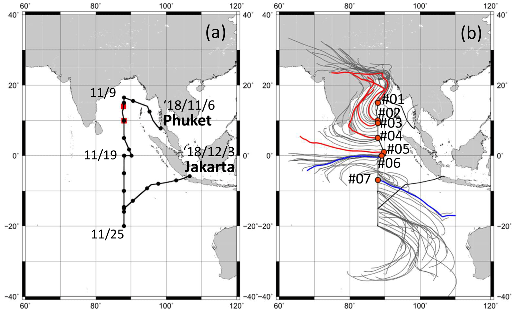
Figure 1 Ship tracks of the KH-18-6 cruise of the RV Hakuho Maru as well as the rain site (a) and 5 d horizontal air-mass backward trajectory (b). The black dots in (a) represent 00:00 of each day at universal time. The red squares in (a) represent sites where rain was observed. Air-mass backward-trajectory calculations started from 500 m a.s.l. above the site. The thin gray lines show trajectories of every 6 h. The orange circles in (b) represent TEM sampling sites. The red and blue lines show the trajectories for TEM sampling.

2.2 Chemical composition of PM_2.5

We collected PM_2.5 samples on Teflon filters (WP500-50; Sumitomo Electric Fine Polymer, Inc.) and prebaked (900 ^∘C for 3 h) quartz fiber filters (QR-100; Advantec Toyo Kaisha Ltd.) using two high-volume samplers (HV-700F; Shibata Science Co. Ltd.) with a custom-made particle-size separator at about 12 or 24 h intervals at a flow rate of 500 L min⁻¹ on the compass deck located at about 14 m altitude from sea level. Collection of particles from the ship exhaust (the ship's funnel was located at the rear of the sampling position) was avoided carefully: the pumping of aerosol samplers was controlled automatically using a wind sector to operate only when the relative wind direction was −80 to 80^∘ of the bow and when the relative wind speed was higher than 3 m s⁻¹. After collection, the Teflon and quartz fiber filter samples (for ionic species and trace metals) were stored before chemical analyses, respectively, at 4 and −18 ^∘C. Mass concentrations of water-soluble ionic species (Cl⁻, NO${}_{\mathrm{3}}^{-}$, SO${}_{\mathrm{4}}^{\mathrm{2}-}$, Na⁺, NH${}_{\mathrm{4}}^{+}$, K⁺, Mg²⁺, and Ca²⁺) on quartz fiber filter samples (12 samples collected during 8–28 November 2018) were analyzed using ion chromatography. Non-sea-salt (nss) concentrations of SO${}_{\mathrm{4}}^{\mathrm{2}-}$, K⁺, and Ca²⁺ were estimated from Na⁺ concentrations in the samples using the bulk seawater ratios described by Wilson (1975). Metals in PM_2.5 (Na, Al, K, Ca, Ti, V, Mn, Fe, Ni, and Zn) were analyzed using inductively coupled plasma mass spectrometry (ICP-MS, 7700X, G3281A; Agilent Technologies, Inc.) with microwave-assisted extraction in a mixture of nitric acid, hydrofluoric acid, and hydrogen peroxide using the Teflon filter sample (14 samples collected during 8–30 November 2018).

2.3 Individual particle analyses using an electron microscope

2.3.1 Observation and elemental analysis

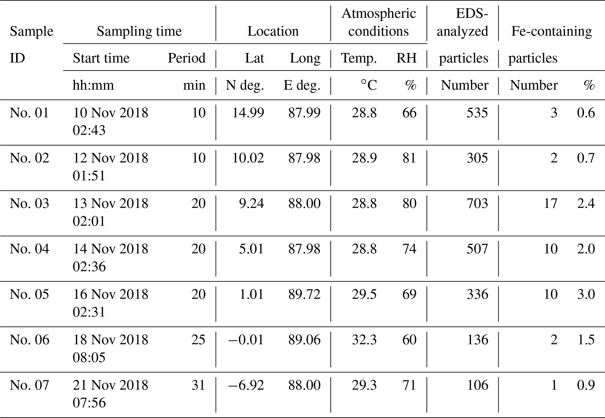
After diffusion drying, aerosols were collected on carbon-coated nitrocellulose (collodion) films using cascade impactors. Then the morphologies and compositions of particles were analyzed using TEM. The aluminum cascade impactor designed by the authors has three impaction stages, each with a single jet nozzle. The respective nozzle diameters for stages 1, 2, and 3 were 1.2, 0.8, and 0.4 mm. The 50 % cutoff diameters at a flow rate of 1.0 L min⁻¹ were, respectively, 1.6, 0.9, and 0.3 µm, as calculated based on Eq. (5.28) presented by Hinds and Zhu (2022). Aerosol samples were collected on the compass deck at the upwind side of the ship for 10–30 min. About one to two TEM samples were taken per day. They were stored under dry conditions at room temperature (about 25 ^∘C) until TEM analyses were conducted at Nagoya University. For this study, seven samples (nos. 01–07) of stage 3 were used for analyses. Sample collection sites and 5 d backward trajectories are presented in Fig. 1b. Sample details are presented in Table 1.

Table 1 TEM samples used for this study, analyzed particles, and Fe-containing particle numbers.

Particles collected on the collodion film were photographed using TEM (200 keV, JEM-2100 Plus; JEOL Ltd.) at 1200 × and 6000 × magnifications. To measure the heights of individual particles on the collection surface, particles were coated with a $\mathrm{Pt}/\mathrm{Pd}$ alloy at a shadowing angle of 26.6^∘ (arctan 0.5) before being micrographed. The $\mathrm{Pt}/\mathrm{Pd}$ coating thickness was about 7 Å. The EDS analyses were conducted using TEM operated in STEM mode at 200 keV. The EDS hyperspectral imaging (HSI) data were sampled at greater than 20 000 magnification for 10–30 frames (20 s per frame) and were kept for each dot of 256×256 pixels using software (NSS3; Thermo Fisher Scientific Inc., Hampton, NH, USA). The dot size was 26×26 nm in the observed field at 20 000 magnification. Although estimating the mass of each element from EDS analysis is difficult, software can estimate the mass fraction (MF_X) of an element X of all analyzed elements from measurement results of X-ray counts as values relative to detected elements. Elemental analyses were conducted fundamentally for C, N, O, Na, Mg, Al, Si, P, S, Cl, K, Ca, Ti, V, Mn, Fe, Cu, Zn, Pd, and Pt. Although the software can identify other elements automatically if EDS spectra have specific X-ray peaks, other elements were detected only rarely. The X-ray count sensitivity when detected using an EDS analyzer depends on the analytical conditions for analyses, such as the frame number and adjustment of the electron beam and detector. Because some conditions can change, evaluating the X-ray count values as absolute values is difficult for samples analyzed on different days or under different settings. Although estimating the mass of each element is not possible, analyzing EDS spectra using software can estimate the mass fraction (MF) of each element from measurement results of X-ray counts as values relative to the selected elements. The mass fraction of element X is described as shown below.

$$\begin{array}{}\text{(1)}& {\mathrm{MF}}_X={\displaystyle \frac{m_X}{m_{\mathrm{total}}}}\end{array}$$

Therein, m_X and m_total, respectively, represent the mass of an element X in a selected area and the mass of all analyzed (selected) elements in the area. For this study, TEM samples were coated uniformly by $\mathrm{Pd}/\mathrm{Pd}$ using the shadowing method before water dialysis. Usually, Pd is not included in general aerosols. Sample nos. 01–07 were vapor deposited by $\mathrm{Pt}/\mathrm{Pd}$ at one time. Therefore, the MF_X value standardized by MF_Pd, $X/\mathrm{Pd}$, can be regarded as a value that is independent from m_total, which changes according to the aerosol composition, collodion film thickness, and distance from the Cu grid.

$$\begin{array}{}\text{(2)}& X/\mathrm{Pd}={\displaystyle \frac{{\mathrm{MF}}_X}{{\mathrm{MF}}_{\mathrm{Pd}}}}={\displaystyle \frac{m_X}{m_{\mathrm{Pd}}}}\end{array}$$

To obtain the elemental compositions of individual particles, the MF_X of each element was obtained manually for selected areas according to the particle shape and size. Background noise effects were eliminated using X/Pd. If the difference between the X/Pd value of a particle area and that of a near background area was greater than 3 standard deviations of multiple background spectra in the same sample, then the value was treated as a significant spectrum of the particle.

2.3.2 Water dialysis and estimation of the water-soluble Fe fraction (f_WSFe)

For samples collected from the Indian Ocean (sample nos. 01–05) north of the Equator, a water dialysis technique (Mossop, 1963; Okada, 1983; Okada and Hitzenberger, 2001; Ueda et al., 2011a, b) was applied to observe and estimate the volume fraction of water-soluble and water-insoluble materials in particles. The TEM grid with particle samples was floated on an ultrapure water drop (approximately 0.3 mL) on a Petri dish at about 25 ^∘C for 3 h with the collection side upward. After water dialysis, some areas were photographed again. Unfortunately, a large part of the collodion film tore during water dialysis. For sample no. 03 only, some EDS analysis data for Fe-containing particles were obtained from the same particle area after water dialysis.

For this study, we expanded the water dialysis technique and EDS analysis to quantify changes in the fraction of water-soluble Fe to total Fe in individual Fe-containing particles. Because Pd is a water-insoluble material coated onto the top surface of samples for this study, the mass of Pd for a selected area after water dialysis (m_{Pd_after}) can be regarded as equivalent to that for the same area before water dialysis (m_{Pd_before}).

$$\begin{array}{}\text{(3)}& m_{\mathrm{Pd}\mathrm{\_}\mathrm{before}}=m_{\mathrm{Pd}\mathrm{\_}\mathrm{after}}\end{array}$$

The fraction of the water-insoluble Fe (WIFe) mass to the total Fe mass in a particle, f_WIFe, can be represented as

$$\begin{array}{}\text{(4)}& f_{\mathrm{WIFe}}={\displaystyle \frac{m_{\mathrm{WIFe}}}{m_{\mathrm{Fe}}}}\times \mathrm{100}\left[\mathit{\%}\right]={\displaystyle \frac{m_{\mathrm{Fe}\mathrm{\_}\mathrm{after}}}{m_{\mathrm{Fe}\mathrm{\_}\mathrm{before}}}}\times \mathrm{100}\left[\mathit{\%}\right],\end{array}$$

where m_{Fe_before} and m_{Fe_after}, respectively, denote the Fe mass before and after water dialysis for an Fe-containing particle. Under Eq. (3), Eq. (4) can be described using $\mathrm{Fe}/\mathrm{Pd}$ before and after water dialysis of the same area for an Fe-containing particle (respectively, $\mathrm{Fe}/\mathrm{Pd}$_before and $\mathrm{Fe}/\mathrm{Pd}$_after), which is based only on measurable values.

$$\begin{array}{}\text{(5)}& f_{\mathrm{WIFe}}={\displaystyle \frac{\mathrm{Fe}/{\mathrm{Pd}}_{\mathrm{after}}}{\mathrm{Fe}/{\mathrm{Pd}}_{\mathrm{before}}}}\times \mathrm{100}\left[\mathit{\%}\right]\end{array}$$

Finally, the fraction of water-soluble Fe to total Fe in a particle, f_WSFe, can be estimated as presented below.

$$\begin{array}{}\text{(6)}& f_{\mathrm{WSFe}}=\mathrm{100}-f_{\mathrm{WIFe}}\left[\mathit{\%}\right]\end{array}$$

2.4 Global model simulation of Fe

We conducted global model simulations using the Community Atmosphere Model version 5 with the Aerosol Two-dimensional bin module for foRmation and Aging Simulations (CAM–ATRAS), with modifications for particulate iron (Matsui et al., 2014, 2018a; Matsui and Mahowald, 2017; Matsui, 2017; Liu and Matsui, 2021a, b; Liu et al., 2022). The model setting for this study was described by Liu et al. (2022). Briefly, the model incorporates emissions, gas-phase chemistry, condensation or evaporation of inorganic and organic species, coagulation, nucleation, activation of aerosols and evaporation from clouds, aerosol formation in clouds, dry and wet deposition, aerosol optical properties, aerosol–radiation interactions, and aerosol–cloud interactions. Aerosol particles were resolved with 12 size bins from a 0.001 to 10 µm dry diameter. The model was run with horizontal resolution of 1.9^∘ × 2.5^∘ and 30 vertical layers from the surface to approximately 40 km. The near-surface layer of model results was used for this study.

The model explicitly treats Fe from biomass burning and anthropogenic combustion. Five Fe sources and minerals (biomass burning and four anthropogenic Fe sources (magnetite (Fe₃O₄), hematite (Fe₂O₃), kaolinite (Al₂Si₂O₅(OH)₄), and illite ((K, H₃O)(Al,Mg,Fe)₂(Si, Al)₄O₁₀)) are considered in addition to eight other aerosol species: sulfate, nitrate, ammonium, dust, sea salt, primary and secondary organic aerosol, black carbon, and water. The anthropogenic Fe emission inventory developed by Rathod et al. (2020) with the update by Liu et al. (2022) for southern Africa was used to model global-scale atmospheric iron concentrations. The size distribution of anthropogenic Fe was referred from observation results reported by Moteki et al. (2017) from aircraft measurements using a single-particle soot photometer for magnetite over eastern Asia. Iron emissions from combustion from open biomass burning were calculated based on a report by Luo et al. (2008). Dust Fe was not treated in our model, but we assumed a constant iron content of 3.5 % in natural dust (Duce and Tindale, 1991; Jickells et al., 2005; Shi et al., 2012).

3 Results and discussion

3.1 Horizontal variation in PM_2.5 components

Figure 2 shows horizontal distributions of the mass concentrations of nss SO${}_{\mathrm{4}}^{\mathrm{2}-}$, NH${}_{\mathrm{4}}^{+}$, and Fe in PM_2.5. The values are shown as mass mixing ratios (the measured mass concentration divided by the atmospheric density (1.18–1.21 kg m⁻³) calculated using the daily average of temperature and atmospheric pressure measured on board), with the same unit of model output, as discussed later (Sect. 3.4). The 25th percentile and the 75th percentile mass concentrations of ions and metals north and south of the Equator at 87–90^∘ E are presented, respectively, in Tables 2 and 3. Scatterplots showing concentrations of Fe and the other elements are presented in Figs. S1 and S2 in the Supplement. Among the measured ions in PM_2.5, the sum of the mass fractions of nss SO${}_{\mathrm{4}}^{\mathrm{2}-}$, NH${}_{\mathrm{4}}^{+}$, Na⁺, and Cl⁻ was larger than 84 % of the total ion mass concentration. North of the Equator, the nss SO${}_{\mathrm{4}}^{\mathrm{2}-}$ and NH${}_{\mathrm{4}}^{+}$ concentrations were especially high. These mass fractions were, respectively, 70 %–76 % and 18 %–22 %, except for data of 11 November 2018, when nss SO${}_{\mathrm{4}}^{\mathrm{2}-}$ and NH${}_{\mathrm{4}}^{+}$ were less around rain event occurrences (Fig. 1a). The values of nss K⁺ also tended to be higher north of the Equator. South of the Equator, the nss SO${}_{\mathrm{4}}^{\mathrm{2}-}$ and NH${}_{\mathrm{4}}^{+}$ concentrations were lower. Consequently, the fractions of sea salt components (i.e., Na⁺ and Cl⁻) were higher. The PM_2.5 ionic amounts in equivalent concentrations of total cations without H⁺ were comparable to or greater than 75 % of that of total anions (Fig. S1a). For non-sea-salt components, the relations between the doubled nss SO${}_{\mathrm{4}}^{\mathrm{2}-}$ molar concentration and the NH${}_{\mathrm{4}}^{+}$ plus nss K⁺ molar concentration were usually between 1:1 and 2:1 (Fig. S1b), suggesting that nss SO${}_{\mathrm{4}}^{\mathrm{2}-}$ originated from ammonium sulfate, ammonium bisulfate, and potassium sulfate rather than from sulfuric acid.

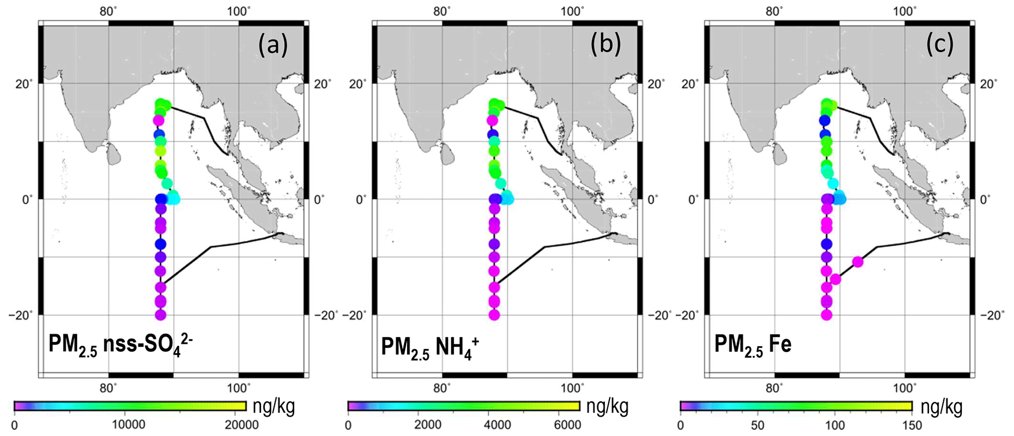
Figure 2 Horizontal variations in mass concentrations of (a) nss SO${}_{\mathrm{4}}^{\mathrm{2}-}$, (b) NH${}_{\mathrm{4}}^{+}$, and (c) Fe in PM_2.5. Each sample was collected continuously for 12 or 24 h under control by the wind sector. Data are shown at averaged locations for latitude and longitude during the sampling period.

Table 2 Average values of PM_2.5 ion mass concentrations at 87–90^∘ E.

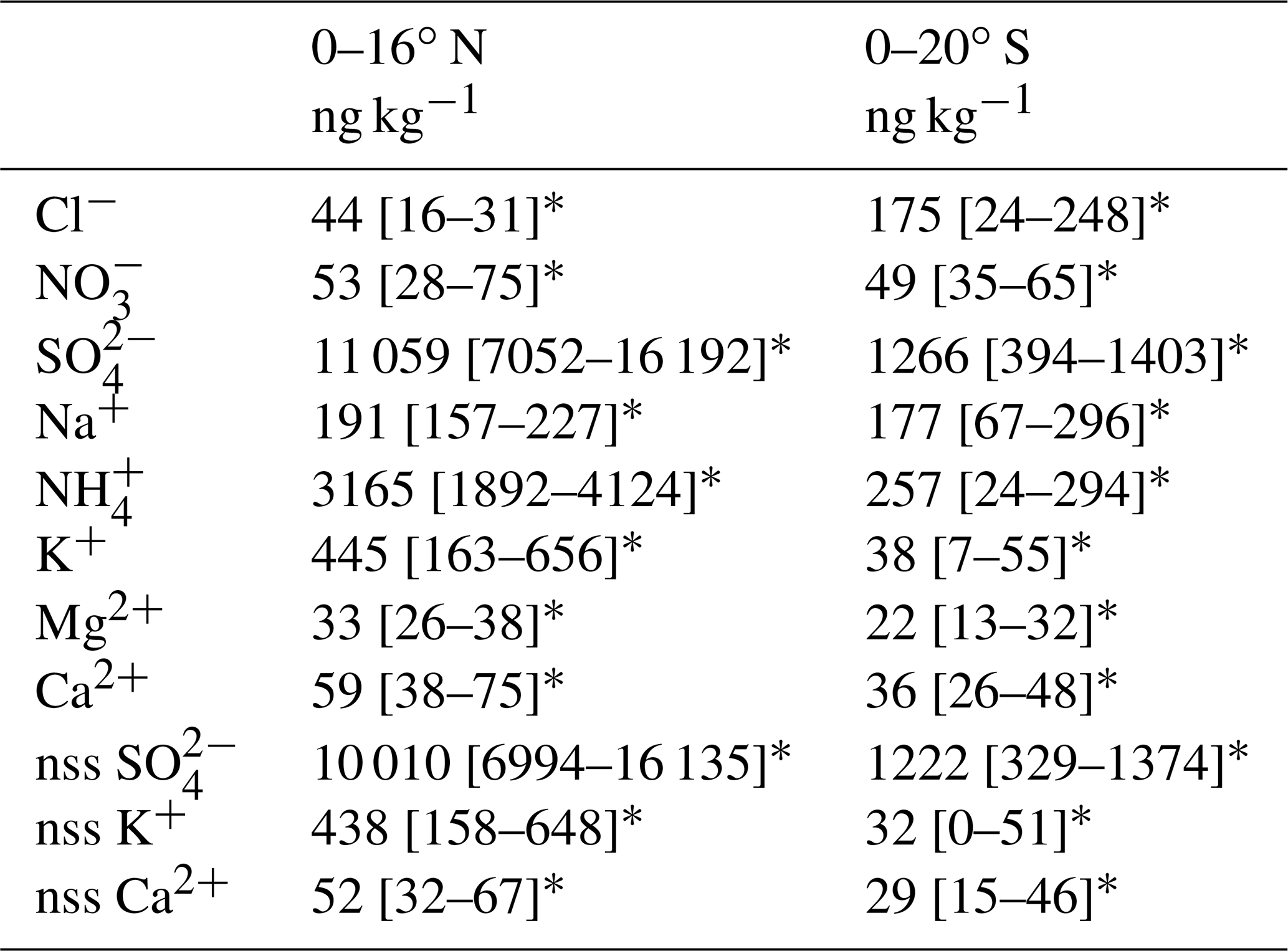
^∗ Values in square brackets are 25th and 75th percentile value ranges.

Table 3 Average values of PM_2.5 metal mass concentrations at 87–90^∘ E.

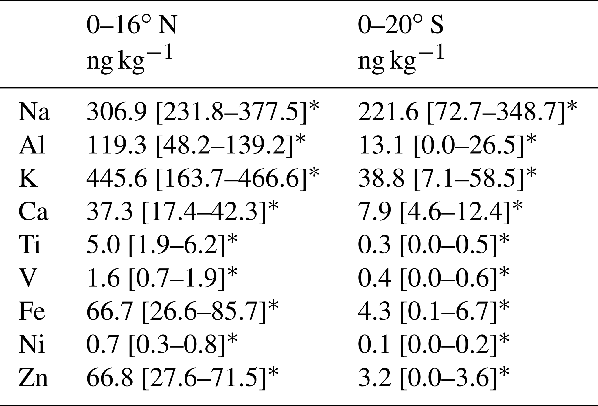
^∗ Values in square brackets are 25th and 75th percentile value ranges.

Among metals measured using ICP-MS, the Na and K mass concentrations were high: 57–1077 ng kg⁻¹ and 5–1023 ng kg⁻¹, respectively. The Fe concentrations were high (10–137 ng kg⁻¹) north of the Equator but low (< 19 ng kg⁻¹) south of the Equator. The Fe mass concentrations were positively well correlated with nss K⁺ (R²=0.95), nss SO${}_{\mathrm{4}}^{\mathrm{2}-}$ (R²=0.93), and Ca (R²=0.90) mass concentrations (Fig. S2). The concentrations of V and Ni, which originate from heavy oil combustion by ships, were closely correlated (R²=0.96). However, their correlations with Fe concentration (R² values of 0.69 and 0.83, respectively) were weaker than the correlation between V and Ni or the correlations of Fe found with nss K⁺, nss SO${}_{\mathrm{4}}^{\mathrm{2}-}$, and Ca. These results suggest that a large fraction of the observed Fe had been transported from around the continental atmosphere with dust, nss K⁺, and nss SO${}_{\mathrm{4}}^{\mathrm{2}-}$. However, good correlation with continental elements implies that Fe was transported together with the continental air mass. It does not imply that emission sources for each element are the same. Therefore, details of the composition and morphological features of individual Fe-containing particles were investigated as described hereinafter in the text.

3.2 Individual particle features and co-existing states with Fe of sulfate and soot

Photographs of all samples (nos. 01–07) are presented in Fig. S3. The morphological features of sample nos. 01–06 were similar. Electron microphotographs of samples no. 01 and no. 07 and the number fractions of the morphological types for all samples are presented in Fig. 3. The morphological types were classified based on a report by Ueda et al. (2016) and features of particles on the samples. For sample nos. 01–06, many particles in all samples had a rounded shape (ball) or were clustered into ball shapes (clustered), such as the blue- and white-arrowed particles of sample no. 01 in Fig. 3. Dome-shaped particles have less height to area (dome). Chain aggregation of small globules (ca. 30 nm) is regarded as a particle composed mainly of soot (soot), although they accounted for only a small fraction. For sample no. 07, some particles constructed of cubic parts having a high contrast to an electron beam were also found. They can usually be regarded as sea salt (SS)-shaped.

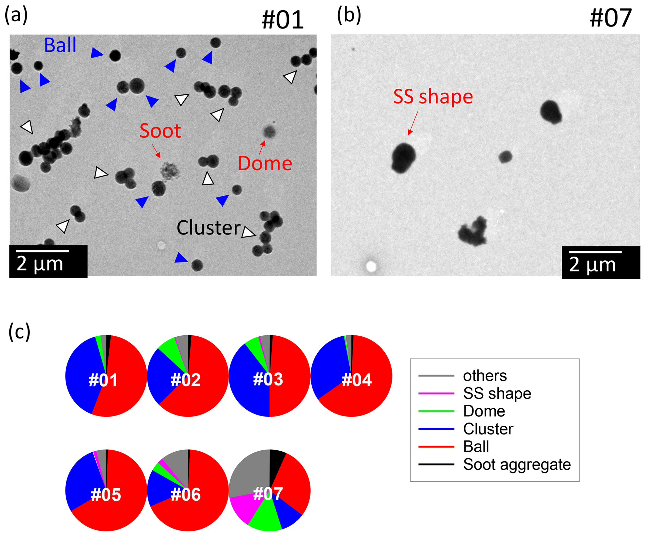
Figure 3 Electron micrographs for sample nos. 01 (a) and 07 (b) and pie charts showing the number fractions of morphological types (c). The blue-arrowed particles are ball-like-shaped particles. The white-arrowed particles are clusters of balls. The red arrows indicate soot as well as dome-shaped and sea-salt (SS)-shaped particles.

Figure 4a portrays a STEM image and EDS mapping of C, O, Al, Si, S, K, Ca, and Fe of an area of sample no. 03 and examples of the X-ray count spectrum for each particle. Ball-like and clustered particles were composed mainly of S, C, and O, indicating sulfate with organic components. K signals in the particles were often found at the same position as the detected S signal. Number fractions of particles detecting each element are depicted in Fig. 5. Moreover, S was detected in > 92 % of all particles for samples collected north of the Equator. K was detected in 16 %–44 % of particles. For other elements, particles containing sea salt (Na, Mg, and Cl) were often detected (in 3 %–48 % of all particles). In addition, Al and Si were detected in about 5 % of particles collected north of the Equator. The findings show that Fe was detected in 1 %–3 % of all particles.

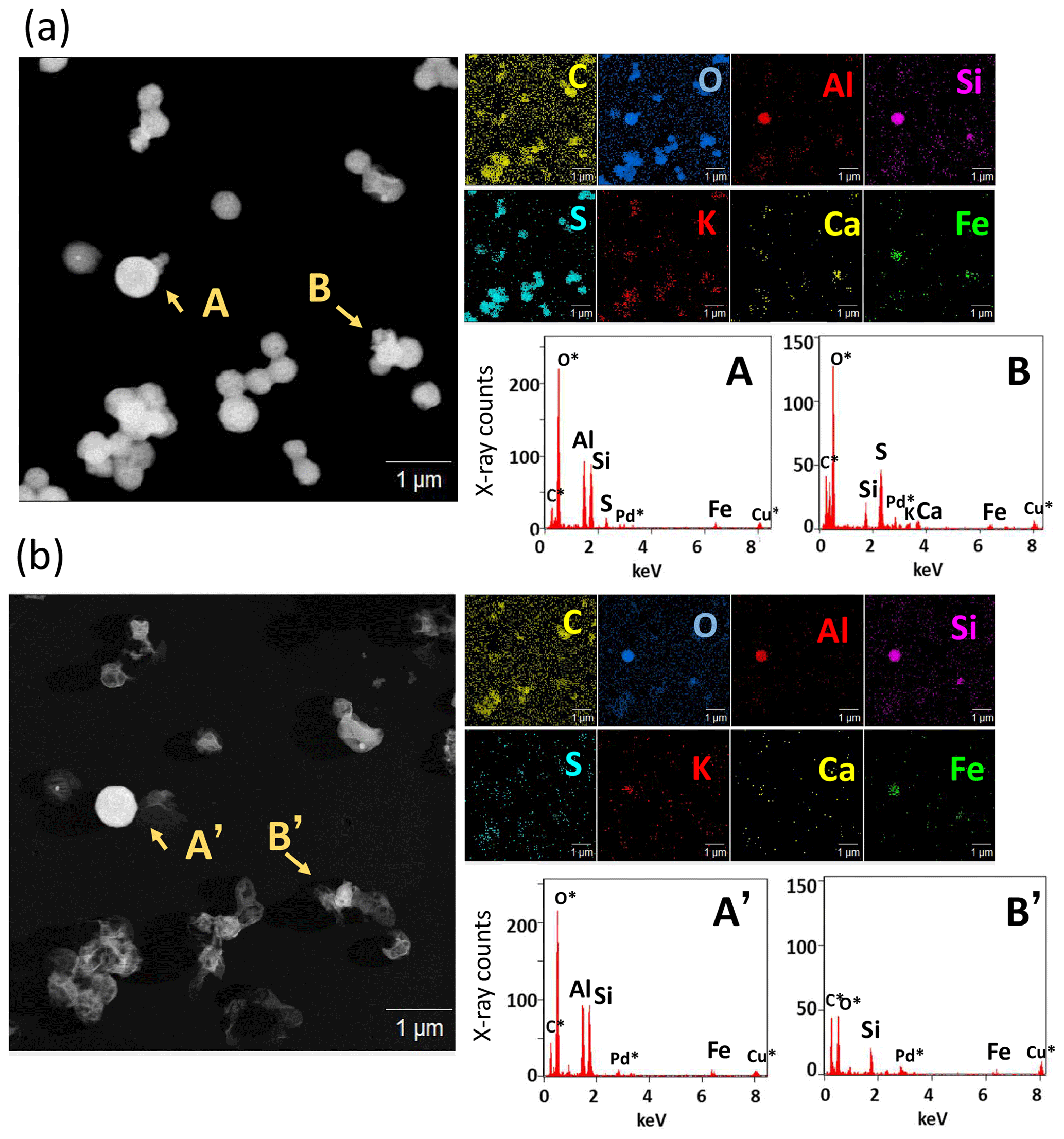
Figure 4 STEM image and an elemental map of sample no. 03 for the same region (a) before and (b) after water dialysis and the extracted X-ray count spectrum for arrowed particles A and B and for the same region after water dialysis (A' and B'). Asterisked (^∗) elements represent elements included in the background area without particles.

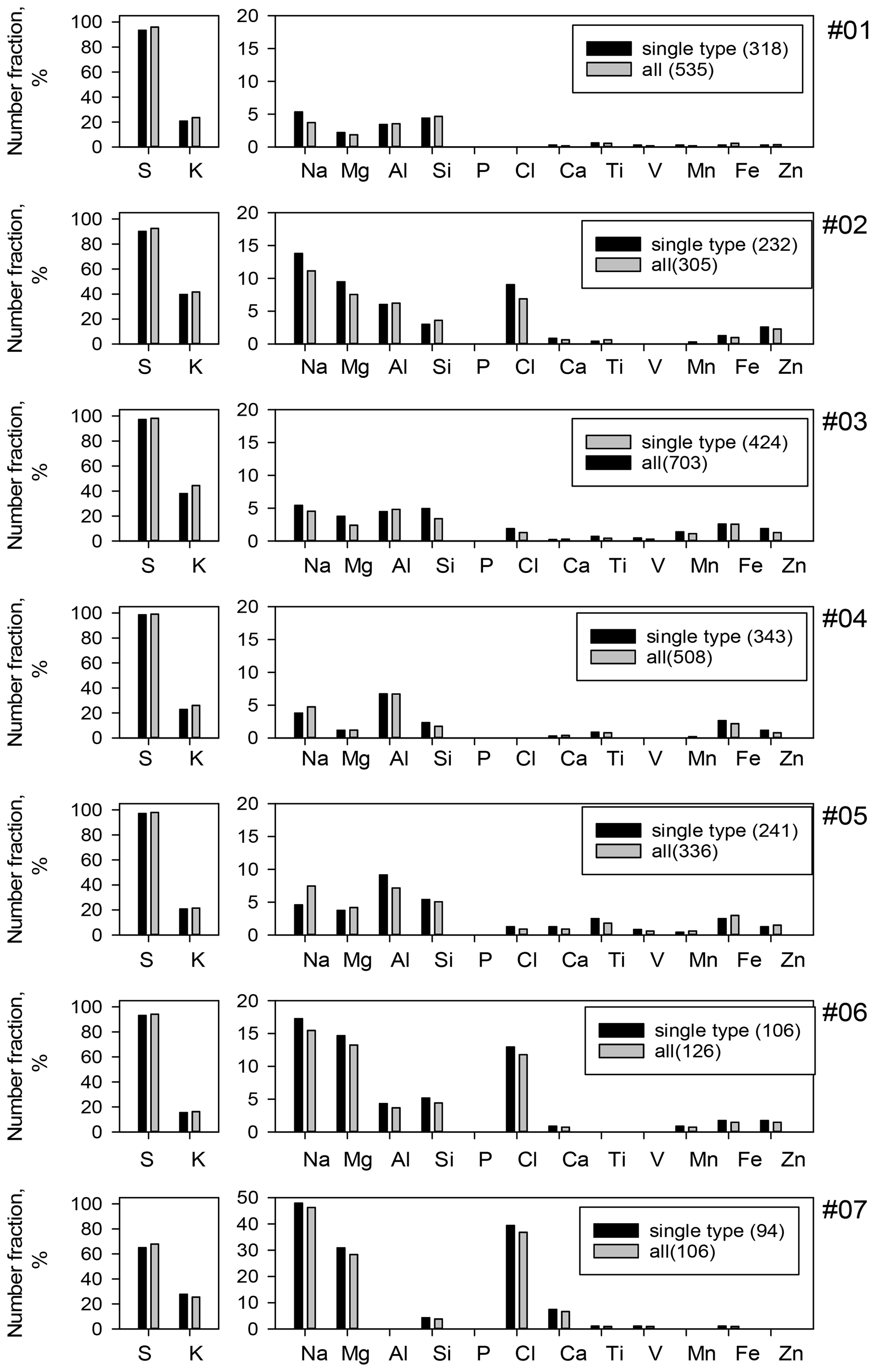
Figure 5 Number fractions of element-containing particles. Single type denotes particles other than cluster-shaped particles. The bracketed numbers in the legend are analyzed particles.

As shown by particles A and B in Fig. 4a, Fe signals were often found from a partial area with attached or coated sulfate. For this study, metal-congested areas containing Fe are designated as Fe-containing parts to distinguish a term from whole particles (Fe-containing particles) such as particles with a co-existing Fe-containing part and sulfate. From some Fe-containing parts, Si, Al, and/or Ca were also detected. Detailed compositions of Fe-containing particles and types of Fe-containing parts are presented hereinafter in the text. Figure 4b shows a STEM image, EDS mapping, and X-ray count spectra after water dialysis for the same area as that portrayed in Fig. 4a. A large part composed of S and K disappeared with dissolution by water dialysis, suggesting that they are water-soluble materials. However, many parts composed of Si, Al, Fe, or C remained on film.

Co-existing Fe-containing parts and sulfate were found from TEM samples. Such sulfates on Fe-containing parts can be formed by condensation from sulfuric gaseous materials or coagulation of sulfate particles. Good correlation between Fe and nss SO${}_{\mathrm{4}}^{\mathrm{2}-}$, as explained in Sect. 3.1, also suggests that a large mass of Fe was transported to the ocean with sulfate particles and their precursor gases. Relations of sulfate particle shapes on samples to their acidity have been reported from some earlier microscopic studies, as explained hereinafter. Acidic sulfate particles such as sulfuric acid (H₂SO₄) and bisulfate (NH₄HSO₄) are usually found as droplets having a satellite structure because of their property of retaining water, even if they were collected after diffusion drying (Waller et al., 1963; Frank and Lodge, 1967; Gras and Ayers, 1979; Bigg, 1980; Ferek et al., 1983). In contrast, particles composed mainly of ammonium sulfate collected after passing the diffusion dryer have been found in the form of ball-like shapes, rectangular regular shapes, and clusters (Ueda et al., 2011b;Ueda, 2021). Most particles of samples examined for this study had a ball-like shape or a cluster. This result indicates that sulfates in the particles were more closely related to neutralized sulfate such as ammonium sulfate than to sulfuric acid, which also corresponds with the result found for PM_2.5, as shown in Sect. 3.1. Particles composed mainly of ammonium sulfate can be present as solid or liquid under a metastable humidity condition between efflorescence and deliquescence humidities, according to their atmospheric humidity experiences. Furthermore, solid ammonium sulfate particles tend to transform to rectangular regular shapes when experiencing metastable humidity conditions (Ueda, 2021). However, rectangular particles were rarely observed in this study, although the atmospheric relative humidity (60 % RH–81 % RH) at the sampling time (Table 1) is usually a metastable condition of ammonium sulfate (35 % RH–80 % RH). Therefore, sulfate particles in our samples are regarded as having existed as droplet particles in the atmosphere.

Based on single soot mass measurement analyses reported by Corbin et al. (2018), much soot originating from combustion of heavy fuel oil in ship engines can include Fe along with V, Na, and Pb. Some soot particles that are less coated by sulfate were also found in our samples. However, metals, including Fe, were not detected from less-coated soot particles in this study, as shown in Fig. S4. For our PM_2.5 result, as explained in Sect. 3.1, Fe was somewhat correlated with V, although the correlation was weaker than that between V and Ni or that between Fe and nss SO${}_{\mathrm{4}}^{\mathrm{2}-}$, nss K⁺, or Ca. In addition to Fe from transport from continental areas, some Fe might have originated in the ship's exhaust, but no strong evidence of ship exhaust contamination was found from our individual particle observations, including analyses of Fe-containing particles presented hereinafter.

3.3 Fe-containing particles: composition and morphological features implying their source

Figure 6a and b portray number fractions of particles containing the respective elements and mixing types with sulfate for Fe-containing particles (42 particles) observed in five samples (nos. 01–05) affected by air masses from south Asia. Most Fe-containing particles were mixed with sulfate (Fig. 6b). Actually, S was detected in 90 % of Fe-containing particles (Fig. 6a). In addition, K was found in half of the Fe-containing particles (Fig. 6a), suggesting that biomass burning affected the Fe-containing particle compositions. However, many K signals were detected from the sulfate coating. Therefore, such a K signal implies secondary formation on Fe-containing parts rather than a source of Fe-containing parts. Both Al and Si were detected in 20 % and 30 % of Fe-containing particles. Very little V originating from heavy oil combustion of ships was detected in Fe-containing particles. Moreover, Na, Mg, Ca, Mn, and Zn were detected in less than 7 %–10 % of Fe-containing particles. Both Ca and Mg can originate from biomass burning in addition to sea salt and mineral dust. Adachi et al. (2022) reported ash-bearing particles found in biomass burning smoke based on TEM analysis of fine (< 2.5 µm) particles. They defined particles containing both Ca and Mg (> 5 weight %) as ash-bearing particles. According to their report, ash-bearing particles from biomass burning smoke commonly exhibit aggregated shapes with complicated compositions, predominantly calcium with other elements (e.g., C, O, Mg, Al, Si, P, S, and Fe). However, in our study, an Fe-containing particle in which both Ca and Mg were detected was only one (2 % of Fe-containing particles). In addition, morphological features of Fe-containing particles were not like those of ash-bearing particles reported by Adachi et al. (2022).

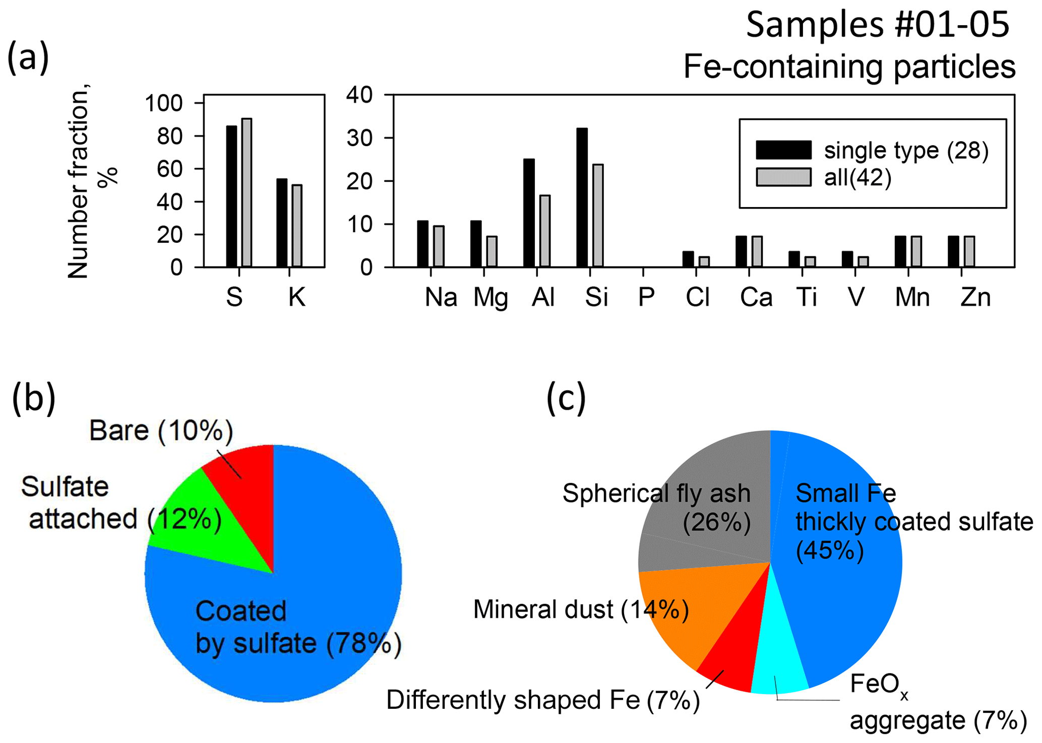
Figure 6 Mixing states and morphological features of Fe-containing particles of samples collected north of the Equator. (a) Number fraction of each element-containing particle in Fe-containing particles. (b) Pie chart of mixing type with sulfate. (c) Pie chart of Fe-containing part types based on constituent elements and morphology. Section 3.3 presents methods of classifying Fe-containing part types. Single type in (a) denotes particles other than cluster-shaped particles.

As shown in Fig. 4a and b, Fe-containing parts had a few different morphological types, such as spherical or irregular shapes and homogeneous or heterogeneous mixing with other elements. Such morphological types can be related to their Fe emission source. Based on the contrast of STEM images and EDS mapping, we divided Fe-containing parts into three morphological types associated with an emission source (spherical fly ash, mineral dust, FeO_x aggregate) and the other two types (differently shaped Fe and small Fe thickly coated by sulfate). The average ± standard deviation values of Fe/Pd for each type above were, respectively, 1.1±2.2, 0.18±0.14, 0.73±0.81, 1.7±0.6, and 0.07±0.05. Number fractions for the morphological types for Fe-containing particles are presented in Fig. 6c. For sample no. 03, the morphological features found after water dialysis were classified. In addition, examples of STEM images, the elemental map, and X-ray spectra for typical Fe-containing particles are portrayed in Fig. 7. Details of the respective morphological types are explained later in Sect. 3.3.1–3.3.4.

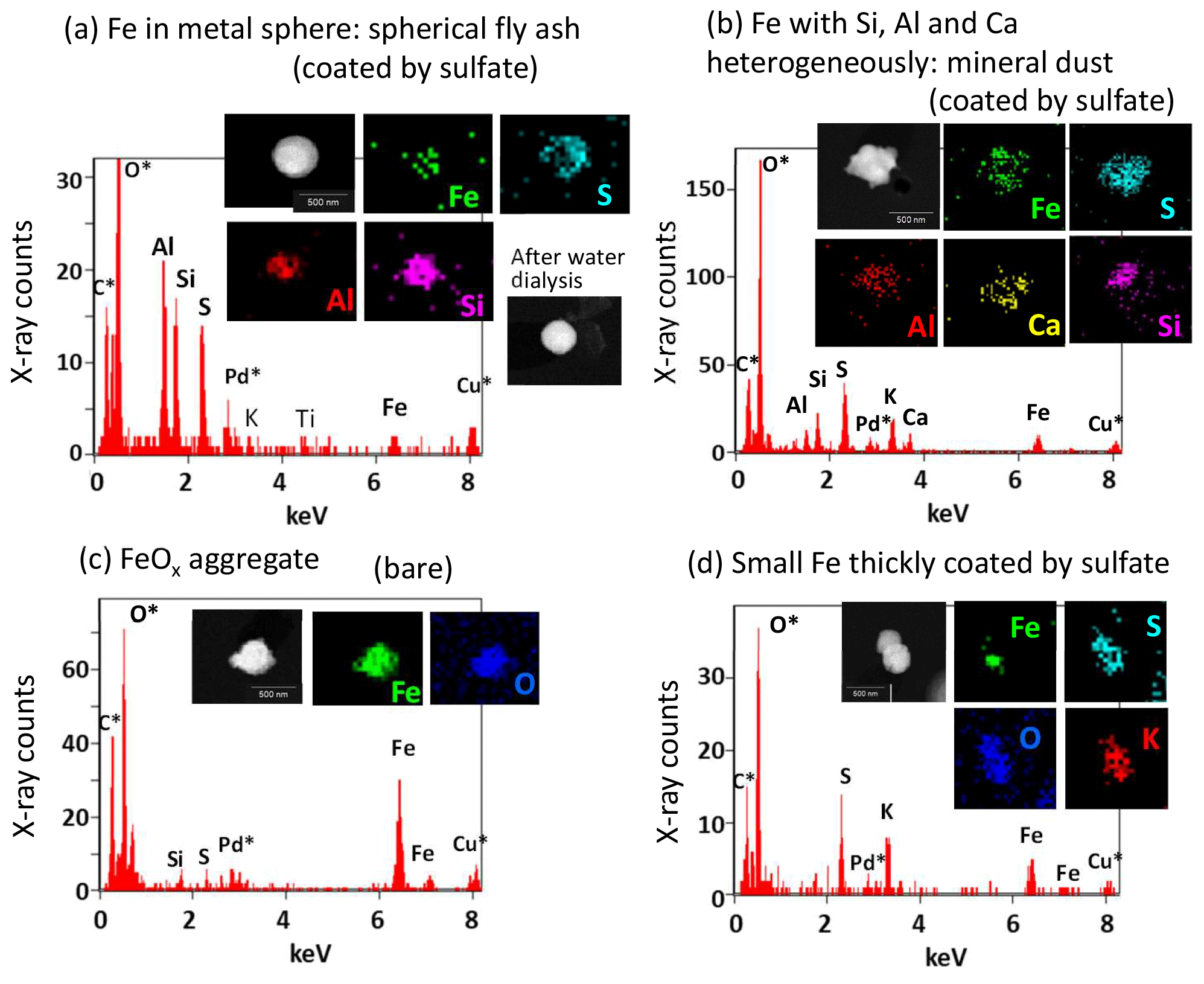
Figure 7 Examples of STEM images, elemental maps, and X-ray count spectra of typical Fe-containing particles. (a) Example of a particle having an Fe-containing part in the metal sphere (spherical fly ash). The metal sphere part of this particle is coated by sulfate. (b) Example of an Fe-containing particle co-existing with Si, Al, or Ca heterogeneously (mineral dust). The Fe, Si, Al, and Ca parts of this particle are coated by sulfate. (c) Example of an FeO_x aggregate particle. (d) Example of a particle having a small Fe-containing part thickly coated by sulfate. Asterisked (^∗) elements in the X-ray count spectrum represent elements included in the background area without particles.

3.3.1 Fe in metal sphere (spherical fly ash)

As shown for particle A in Fig. 4 and for the particle in Fig. 7a, Fe-containing spheres with Al and/or Si were found in nine particles (21 % of Fe-containing particles) from sample nos. 03 and 04, affected by air masses from the eastern coast of India (Table S1 and Fig. 1b). In addition, Fe spheres without Al or Si were found in two particles (5 % of Fe-containing particles) from sample no. 05, affected by air masses from the Maldives. All particles containing metal spheres of both types co-existed with sulfate. In the STEM image, such metal spheres have a high contrast compared with sulfate. Such spheres remained as a residue after water dialysis. Spherical shapes of metals reflect their formation through evaporation at high temperatures and subsequent rapid condensation. Moreover, the shape coincides with often-encountered features of fly ash particles originating from coal combustion at electrical generation facilities (e.g., Fisher et al., 1978; Yao et al., 2015; Umo et al., 2019). For this study, metal spheres composed mainly of Fe, Si, or Al in our atmospheric aerosol samples are designated as spherical fly ash to distinguish them from fly ash related to emission sources that are not classified based on morphological characteristics. In coal, Fe generally exists as pyrite or aluminosilicate (Tomeczek and Palugniok, 2002). Aluminosilicate Fe, such as kaolinite and illite, generally undergoes high-temperature melting and fragmentation, leading to formation to fly ash (Rathod et al., 2020). Although low-temperature combustion processes such as residential uses might not engender Fe volatilization (Flagan and Seinfeld, 2012), power plants can emit large amounts of fly ash (Rathod et al., 2020). Although the mass concentration peak of fly ash emitted from power plants is super-micrometric (1–10 µm), submicrometer fly ash particles are also emitted together. They have been observed and described in the literature (Markowski and Filby, 1985; Liu et al., 2018; Umo et al., 2019).

3.3.2 Fe co-existing with Al, Si, or Ca heterogeneously (mineral dust)

As shown for particle B in Fig. 4 and for the particle in Fig. 7b, some non-spherical parts containing Fe, Si, and Al were also found. Unlike the Fe-containing sphere parts explained earlier, Ca was usually detected from such non-spherical Fe-containing parts. Additionally, they have some domains of different concentrations of Fe, Al, Si, and Ca. The Fe, Al, Si, and Ca are the main elements of silicate minerals. Mineral dust is usually composed of a few different mineral species (Conny, 2013; Jeong and Nousiainen, 2014; Jeong et al., 2014, 2016; Conny et al., 2019; Ueda et al., 2020). Therefore, heterogeneous structures including Fe, Al, Si, Ca, and others imply that they are mineral dusts with no combustion-related origin. Such Fe-containing parts regarded as mineral dust were found in six particles (14 % of Fe-containing particles) in sample nos. 01, 03, 04, and 05 (Table S1). Most particles of this type (five particles) co-existed with sulfate. Based on water dialysis of sample no. 03, Ca in particle B in Fig. 4a dissolved with water dialysis, as portrayed in Fig. 4b. Although calcite in dust is poorly soluble, chemical transformation from calcite into calcium sulfate or calcium nitrate with atmospheric aging can alter its solubility (Okada et al., 1990, 2005; Zhang and Iwasaka, 1999; Matsuki et al., 2005).

3.3.3 FeO_x aggregate

Some aggregate components comprising Fe and O without other metals were found as shown for a particle in Fig. 7c. They are regarded as being FeO_x, such as magnetite and illite. Similar aggregated FeO_x nanoparticles have been reported by several studies applying electron microscopy to the observation of urban atmospheres (Hu et al., 2015; Adachi et al., 2016; Ohata et al., 2018), roadside environments (Sanderson et al., 2016), and polluted remote seas (Li et al., 2017). Aggregated FeO_x co-existing with soot was also found at urban sites (Ohata et al., 2018; Ueda et al., 2022). From the present study, aggregated FeO_x particles (designated as FeO_x aggregates) were found without a C-rich part in three particles (7 % of Fe-containing particles) in sample nos. 02, 03, and 04, affected by air masses from India (Table S1 and Fig. 1). Two FeO_x aggregates co-existing with sulfate were found. As explained in Sect. 3.2, soot-containing metals were also minor. Actually, FeO_x can be emitted from blast furnaces at iron-smelting facilities (Machemer, 2004) and as exhaust from motor vehicles (Kukutschová et al., 2011; Liati et al., 2015). However, considering FeO_x without soot, FeO_x aggregates examined for this study might have originated mainly from the former source.

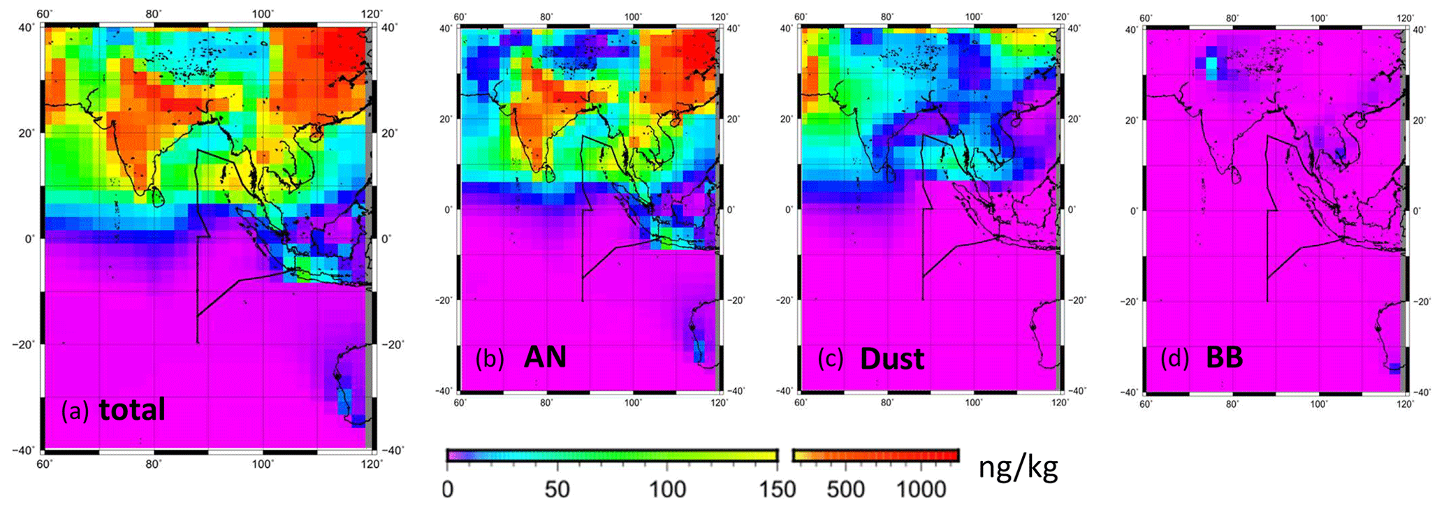
Figure 8 Spatial distributions of PM_2.5 Fe mass concentrations simulated using the CAM–ATRAS model for (a) total, (b) anthropogenic (AN), (c) mineral dust (Dust), and (d) biomass burning (BB) Fe. Values are monthly averaged surface mass concentrations for November 2018.

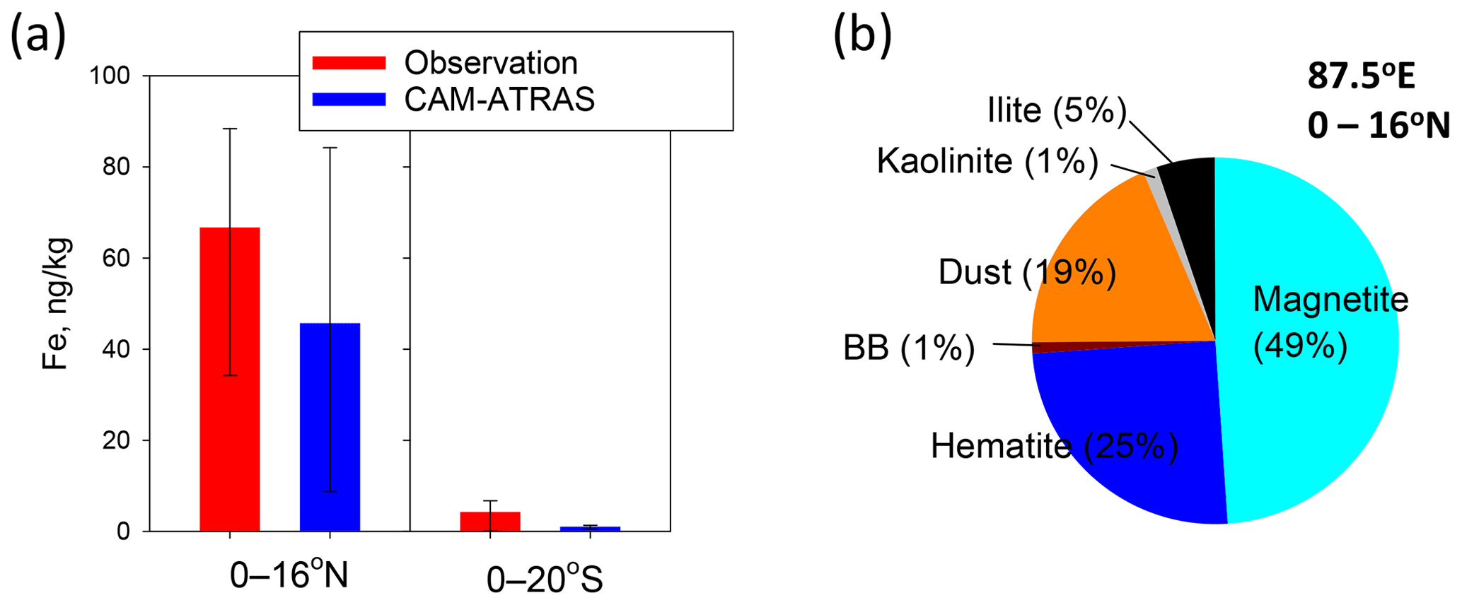
Figure 9 PM_2.5 Fe mass concentrations simulated by CAM–ATRAS. (a) Averaged PM_2.5 Fe simulated value for 87.5^∘ E and observed PM_2.5 Fe of 87–90^∘ E during the KH-18-6 cruise. The lower and upper error bars, respectively, stand for the 25th and 75th percentiles. (b) Pie chart of averaged mass fraction simulated PM_2.5 Fe for each Fe species of 0–16^∘ N at 87.5^∘ E. Simulated values are monthly averaged mass concentrations for November 2018.

3.3.4 Differently shaped Fe and small Fe thickly coated by sulfate

For Fe-containing parts of three particles (7 % of Fe-containing particles), different shapes were found in terms of the features described above: spherical fly ash, mineral dust, and FeO_x aggregates. They were designated as differently shaped Fe. Of those, two particles were without sulfate. For the other 19 Fe-containing particles, discriminating the shapes of Fe-containing parts was difficult because such parts were much smaller than the sulfate coating, as illustrated in Fig. 7d. Such Fe-containing particles were classified as small Fe thickly coated by sulfate separately from differently shaped Fe. The number fraction was 45 % of the Fe-containing particles. However, the Fe/Pd values (0.07±0.05) from such small Fe were usually less than those of the other types.

3.4 Fe simulation for each source by the global model

To elucidate the origins of Fe and the model performance, Fe simulation results obtained using the CAM–ATRAS model were compared with observation results. Figure 8 shows the monthly mean simulated mass concentrations in PM_2.5 for the total Fe and Fe from each source at the surface. The color scale of 0–150 ng kg⁻¹ is the same as that presented for Fig. 2c. The averages of the total Fe mass concentrations for areas north and south of the Equator along the ship tracks (0–16^∘ N and 0–20^∘ S at 87.5^∘ E) are shown in Fig. 9a with the observed values. The averages of observed values and model results were, respectively, 66.7 and 45.7 ng kg⁻¹ at 0–16^∘ N and 4.3 and 1.0 ng kg⁻¹ at 0–20^∘ S. The model simulations reproduce the contrast of the Fe mass that was found north (high concentration) and south (low concentration) of the Equator during the cruise well. Although the simulated Fe mass tends to be lower than the observed Fe mass (Fig. 9a), our simulations using the recent anthropogenic Fe inventory data reported by Rathod et al. (2020) show higher Fe mass concentrations and better agreement with observations than earlier estimates producing older emission inventories (Liu et al., 2022). Large uncertainties exist in Fe emission inventories from all sources, including anthropogenic sources, dust, and biomass burning. Moreover, the different spatial and temporal scales found between observation and models might influence the comparisons presented herein.

The CAM–ATRAS results show that anthropogenic Fe was dominant in the PM_2.5 Fe concentration within the area presented in Fig. 8. The averaged mass fractions of Fe source/mineral types in the model estimated for 0–15^∘ N at 87.5^∘ E are depicted in Fig. 9b. The anthropogenic Fe (magnetite, hematite, illite, and kaolinite), dust Fe, and biomass burning Fe were, respectively, 80 %, 19 %, and 1 % of the mass of PM_2.5 Fe. In particular, anthropogenic Fe around India has a high concentration in Fig. 8, suggesting that the anthropogenic activities taking place in that area affected Fe concentrations over the Indian Ocean.

Anthropogenic Fe was mostly (74 % in mass of PM_2.5 Fe) estimated as FeO_x (magnetite and hematite). The mass fraction of anthropogenic aluminosilicate Fe (illite and kaolinite), which mainly derives from coal combustion, was only 6 % in the model. These simulation results can be expected to underestimate the fraction of aluminosilicate Fe and to overestimate the fraction of FeO_x compared with the TEM results. In the TEM samples, spherical fly ash having sufficient Fe/Pd values was often found (26 % of Fe-containing particles), as depicted in Fig. 6. In addition, most of the fly ash particles (8 in 11 spherical fly ash particles) contained Al and/or Si. The mineralogy of Fe from coal combustion in the emission inventory by Rathod et al. (2020), which is used in our model, was estimated from a reference to mineralogical measurements of bulk samples using Mössbauer spectrometry or from the X-ray absorption near-edge structure. Although fuels and combustion temperatures can affect the mineralogical transformation from fuels to by-products, the Fe contents estimated from mineralogical measurements of coal fly ash at electrical generation facilities tend to include both oxides (such as magnetite and hematite) and clay (such as kaolinite and illite) (Hinckley et al., 1980; Szumiata et al., 2015; Waanders et al., 2003; Oakes et al., 2012; Rathod et al., 2020). However, even if Fe in spherical fly ash in our TEM samples were assumed to be composed of aluminosilicates and equivalent FeO_x, the mass fraction of aluminosilicate Fe inferred from TEM results would be larger than 13 %, which is higher than our model-simulated findings. Multiple factors such as the fossil fuel composition and combustor can affect the chemical composition and size–mass distribution of coal fly ash particles at the source (Markowski and Filby, 1985; Liu et al., 2018). The lack of clarity in assessing those factors can also affect the uncertainty in the simulation for the emissions of Fe originating from coal combustion and transport according to the particle size. Such underestimation of aluminosilicates is expected to be one factor causing the underestimation of the total Fe mass concentration in our model.

3.5 Water solubility of Fe

Figure 10 portrays the relation between Fe/Pd before and after water dialysis (14 particles) for sample no. 03. The symbols were made according to the composition and shape of residues after water dialysis. For particles containing metal sphere residues regarded as fly ash, the values of Fe/Pd after water dialysis presented in Fig. 10a and b correspond well to the values found before water dialysis at a 1:1 ratio. Because the Pd mass after water dialysis can be regarded as equal to that before water dialysis, such a 1:1 relation indicates the Fe in spherical fly ash as almost insoluble in water. For particles aside from metal spheres containing residues, the detected values of Fe/Pd decreased, suggesting that some Fe contents are soluble in water. Figure 11 portrays f_WSFe for Fe-containing particles on sample no. 03. The averages of f_WSFe were 48 %, 6 %, 58 %, and 65 %, respectively, for all Fe-containing particles, spherical fly ash, mineral dust, and Fe-containing particles except spherical fly ash.

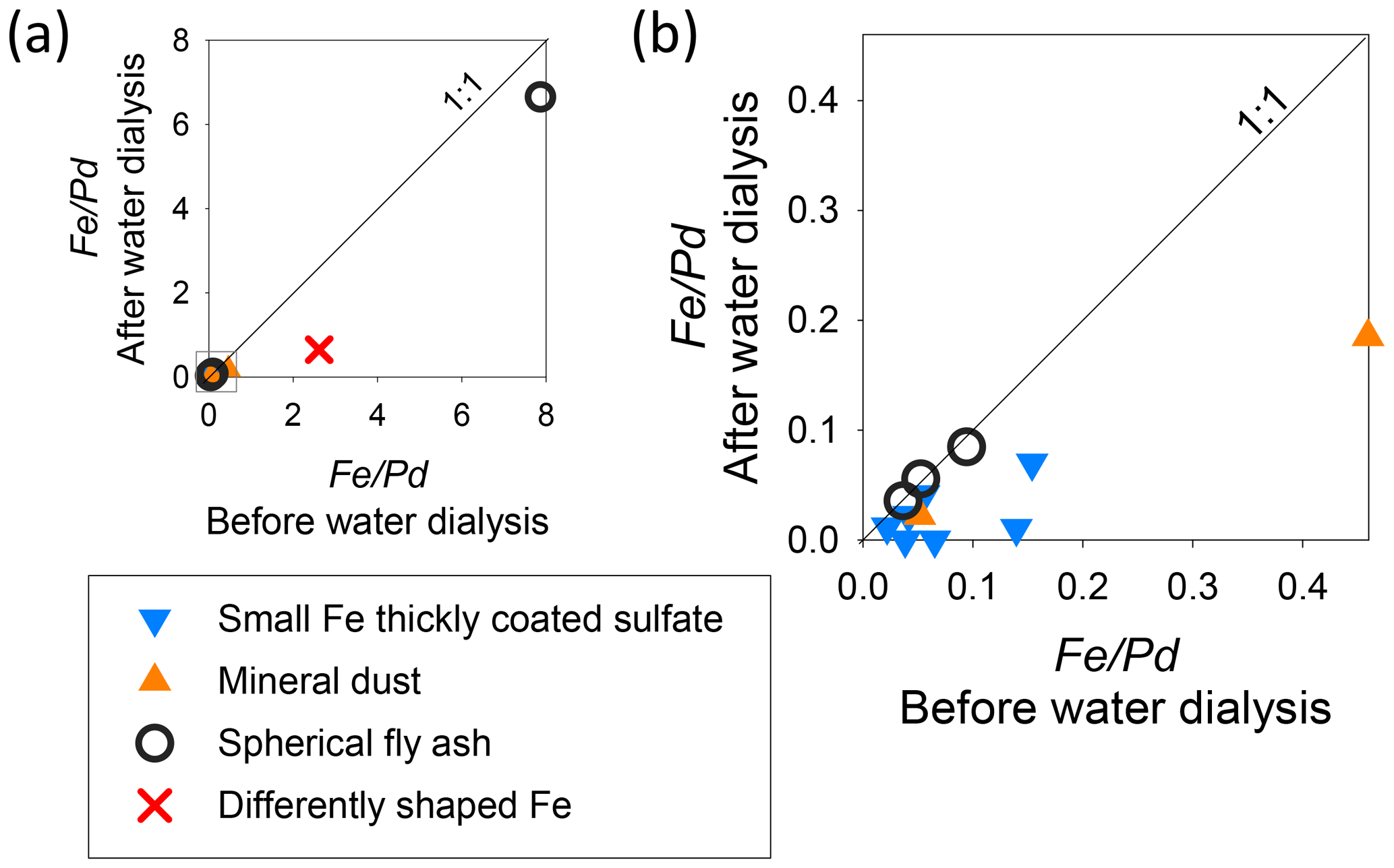
Figure 10 Scatterplot of the $\mathrm{Fe}/\mathrm{Pd}$ before and after water dialysis for Fe-containing particles on sample no. 03. Panel (b) shows an enlarged graph of the light gray square area of panel (a). Pd is a coating material in alloy for giving shadowing to samples.

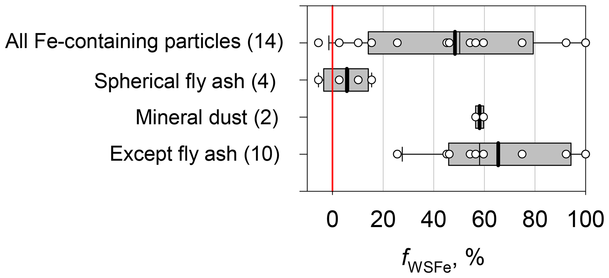
Figure 11 Boxplot of the water-soluble Fe fraction (f_WSFe) of Fe-containing particles for sample no. 03. The lower boundary of the box shows the 25th percentile. The line within the box represents the median. The upper boundary of the box stands for the 75th percentile. The whiskers above and below the box, respectively, show the 90th and 10th percentiles. The white circles show values for the respective particles.

Some measurement-based studies examining bulk aerosol samples have reported fractions of water-soluble Fe in all Fe (Kumar and Sarin, 2010; Baker et al., 2013; Ingall et al., 2018). After Kumar and Sarin (2010) also measured Fe in PM_2.5 at a high-altitude site in a semi-arid region of western India, they reported fractions of water-soluble Fe as 0.06 %–16.1 %. Ingall et al. (2018) measured the water solubility of total Fe in bulk aerosol samples taken from multiple locations in the Southern and Atlantic oceans, Noida (India), Bermuda, and the eastern Mediterranean (Crete). Their fractions of water-soluble Fe were low (< 5 %) under samples influenced by Saharan dust, but the fractions for samples from Noida (3 %–20 %) and samples influenced from Europe were high (17 %–35 %), indicating an anthropogenic contribution of soluble Fe. From measurements taken of the remote ocean, Baker et al. (2013) reported an Fe solubility of 2.4 %–9.1 % for aerosol collected in the Atlantic Ocean during research cruises. Compared with the Fe solubility found from the studies described above, the water-soluble Fe fraction for individual Fe-containing particles in this study tended to be estimated as higher. This finding could be attributed to the fact that our analyzed samples comprised smaller particles (0.3–0.9 µm sample stage diameter) with a greater surface relative to the particle mass and aged particles collected over the remote ocean, as explained below.

The values of f_WSFe found from this study were 20 %–100 % in Fe-containing particles, except for spherical fly ash. Among Fe-containing minerals, the fractions of water-soluble Fe in FeO_x (magnetite, goethite, and hematite) and clays (e.g., kaolinite and illite) are very low (respectively, < 0.01 % and 1.5 %–4 %), but those of ferrous and ferric sulfate are higher (50 %–90 %) (Desboeufs et al., 2005; Journet et al., 2008; Schroth et al., 2009; Rathod et al., 2020). The Fe solubilities for many Fe-containing particles in this study were comparable with those of ferrous and ferric sulfates. Our earlier study found non-/less-sulfate-coated FeO_x in aerosol samples collected in urban Tokyo, for which we applied the same analysis (Ueda et al., 2022). However, few decreases in Fe with water dialysis were found. The difference in Fe solubility found from this urban study can be attributed to atmospheric aging processes because of the coating of secondary aerosol materials and Fe oxidation during transport. Some results of experimentation and simulation studies have shown that Fe in minerals composed of Fe oxide and clays can be oxidized and enhanced in an acidic liquid phase, such as in aerosol droplets and clouds (Shi et al., 2009, 2015; Chen et al., 2012). For the present study, most of the observed Fe-containing particles co-existing with sulfate were regarded as droplets in the atmosphere. Therefore, Fe in particles was regarded as being oxidized in liquid droplet particles in the atmosphere, after which they were collected as water-soluble Fe, such as Fe sulfate. For Fe-containing particles in this study, the number fraction of FeO_x aggregates was smaller, whereas that of categorized particles to small Fe thickly coated by sulfate was higher. The loss of the water-insoluble Fe shape occurring because of the change to water-soluble Fe can be expected to affect this result.

All water-insoluble residues in Fe-containing particles of f_WSFe<15 % were spherical fly ash. Although all of them co-existed with sulfate, water dialysis results indicated that they retained the water insolubility of Fe. Our observed insoluble sphere residues imply structural and morphological features as reasons for the insolubility of the Fe contained in aged fly ash particles. Spherical particles have minimal surface area. In addition, their Fe is distributed in particles with other insoluble materials composed of Si and Al in the sphere. This distribution would physically block the oxidation and dissolution of Fe. However, results of several studies have suggested that Fe in similar spherical fly ash particles can dissolve in acidic particles (Chen et al., 2012; Li et al., 2017). Li et al. (2017) observed similar submicrometer Fe-rich spheres coated by sulfate in samples collected over the Yellow Sea affected by the eastern Asian continental outflow. They used nanoscale secondary ion mass spectrometry and elemental mapping with STEM to analyze sulfate-rich particles containing Fe-rich parts and reported the presence of dispersed FeS⁻ (Fe sulfate) around the FeO⁻ (Fe oxide)-rich part. They concluded that such an Fe sulfate was formed from Fe dissolution of fly ash in an acidic aqueous phase because no other atmospheric source of Fe sulfate or process engenders its formation. Using bulk samples of coal fly ash composed mainly of spherical particles, Chen et al. (2012) also investigated Fe dissolution. Their experiments demonstrated that Fe in coal fly ash can dissolve in H₂SO₄ acidic aqueous solutions of pH 1 and 2. These results of earlier studies suggest that some Fe in fly ash can exist as water-soluble Fe in sulfuric acid particles. However, the results of our experiments have indicated that soluble Fe in spherical fly ash was considerably less present or nonexistent compared with insoluble Fe. From the present study, as explained in Sect. 3.2, sulfate particles were found as neutralized particles such as ammonium. Such atmospheric conditions observed in the present study might not have decreased pH sufficiently to enhance the Fe solubility of fly ash.

Our observation results obtained from these TEM samples suggest fly ash as an important component of fine Fe-containing particles. In addition, water dialysis results suggest that Fe in aged particles over the remote ocean tends to exist as partly or mostly water-soluble Fe, whereas Fe in spherical fly ash can maintain water insolubility. Model simulations have led to estimates that FeO_x is a major component in PM_2.5 Fe of this area and that Fe from anthropogenic aluminosilicates from sources such as coal combustion is minor. Underestimation of the mass fraction of Fe which remained water insoluble during atmospheric transport can be a factor affecting the estimation error in water-soluble Fe deposition. In addition, although Fe mineralogy is often used for the simulation of solubility of anthropogenic Fe in percentage terms in some models, the spherical shape of fly ash particles and the results obtained from water dialysis imply that Fe solubility and the change in the atmosphere depend not only on mineralogical features but also on morphological and structural features of fly ash originating from emission processes. The presence of fly ash in fine aerosols should be noted for model simulations of water-soluble Fe and estimations based on size-segregated samples of Fe concentrations.

4 Summary and conclusions

To elucidate the mixing states and the water solubility of Fe-containing particles in remote marine areas, we conducted shipborne aerosol observations over the Indian Ocean during the RV Hakuho Maru cruise. After TEM samples for individual particle analysis were obtained, they were analyzed using EDS and water dialysis. Most of the particles were composed mainly of sulfate neutralized by ammonium or potassium: the particle number fraction, 0.6 %–3.0 %, of particles on a sample stage of 0.3–0.9 µm diameter contained Fe. They mostly included co-existing sulfate.

Air-mass backward-trajectory analyses suggest that air masses south of the Equator were transported from southern India. Both the correlations of the respective elements measured using chemical analysis for bulk PM_2.5 samples and the absence of V and soot for individual Fe-containing particles imply that the Fe in particles was transported mainly from around the continent rather than from ship exhaust. The Fe in particles was found to include the following: 26 % of metal spheres, often co-existing with Al or Si, regarded as fly ash; 14 % as irregularly shaped heterogeneously co-existing with Si, Al, or Ca, regarded as mineral dust; and 7 % as FeO_x aggregates.

Global model simulations using a recent emissions inventory mostly reproduced the observed PM_2.5 Fe concentrations in the north and south during the cruise. The model simulations suggested that PM_2.5 Fe over the observation site was influenced strongly by anthropogenic Fe emissions around India. In contrast, comparison with the morphological features of observed Fe suggests that the simulations overestimate the fractions of anthropogenic FeO_x and underestimate the fraction of Fe in aluminosilicates originating from coal combustion.

Water dialysis analysis of a TEM sample indicates that about half of the Fe in Fe-containing particles was soluble in water. However, Fe in spherical fly ash particles was almost insoluble in water, even when co-existing with sulfate. Dissolution and oxidation of Fe in spherical fly ash were regarded as having been blocked by the small surface of the sphere and the structure of Fe dispersion in other insoluble aluminosilicates.

Our results obtained from shipboard observations and individual fine aerosol analysis indicate that Fe of various types, such as fly ash, FeO_x, and mineral dust, co-exists with sulfate over the remote Indian Ocean and that the solubility of Fe differs among the materials. Although the model simulations show good agreement with the observed Fe mass concentrations, the results indicate marked differences in the mass fractions of mineral sources of model simulations compared with the observed Fe types. Results of earlier studies have demonstrated that anthropogenic fine Fe tends to be composed mainly of FeO_x, with increased solubility occurring along with aging. However, our results suggest that Fe in spherical fly ash can stand out in fine aerosols over the remote ocean and can retain water insolubility. For an accurate estimation of the effects of atmospheric Fe on marine biogeochemical activity, greater attention must be devoted to morphological and mineral types of Fe depending on its source and especially to insoluble Fe in fly ash.