the Creative Commons Attribution 4.0 License.
the Creative Commons Attribution 4.0 License.
 | 29 Jul 2022
The impacts of wildfires on ozone production and boundary layer dynamics in California's Central Valley
Keming Pan
Ian C. Faloona
We investigate the role of wildfire smoke on ozone photochemical production (P(O3)) and atmospheric boundary layer (ABL) dynamics in California's Central Valley during June–September from 2016 to 2020. Wildfire events are identified by the Hazard Mapping System (HMS) and the Hybrid Single Particle Lagrangian Integrated Trajectory Model (HYSPLIT). Air quality and meteorological data are analyzed from 10 monitoring sites operated by the California Air Resources Board (CARB) across the Central Valley. On average, wildfires were found to influence air quality in the Central Valley on about 20 % of the total summer days of the study. During wildfire-influenced periods, maximum daily 8 h averaged (MDA8) O3 was enhanced by about 5.5 ppb or 10 % of the median MDA8 (once corrected for the slightly warmer temperatures) over the entire valley. Overall, nearly half of the total exceedances of the National Ambient Air Quality Standards (NAAQS) where MDA8 O3 > 70 ppb occur under the influence of wildfires, and approximately 10 % of those were in exceedance by 5 ppb or less indicating circumstances that would have been in compliance with the NAAQS were it not for wildfire emissions. The photochemical ozone production rate calculated from the modified Leighton relationship was also found to be higher by 50 % on average compared with non-fire periods despite the average diminution of j(NO2) by ∼ 7 % due to the shading effect of the wildfire smoke plumes. Surface heat flux measurements from two AmeriFlux sites in the northern San Joaquin Valley show midday surface buoyancy fluxes decrease by 30 % on average when influenced by wildfire smoke. Similarly, afternoon peak ABL heights measured from a radio acoustic sounding system (RASS) located in Visalia in the southern San Joaquin Valley were found to decrease on average by 80 m (∼ 15 %) with a concomitant reduction of downwelling shortwave radiation of 54 Wm−2, consistent with past observations of the dependence of boundary layer heights on insolation.
- Article
(3134 KB) - Full-text XML
- BibTeX
- EndNote


Ozone (O3) pollution poses a threat to public health and the environment. Excessive O3 exposure is known to damage the tissues of the respiratory tract causing a variety of symptoms such as chest pain, coughing, emphysema, and asthma, leading to the need for increased medical care (Rombout et al., 1986). Apart from that, O3 also causes substantial damage to crops, forests, and native plants (Ainsworth, 2017). Tropospheric O3 is produced from the chemical reaction of nitrogen oxides (NOx= NO + NO2) and volatile organic compounds (VOCs) in the presence of sunlight. Figure 1 shows the photochemical formation of O3 in the presence of NOx and VOCs (Jenkin and Hayman, 1999). Reactions (R1)–(R5) are the major reactions in this process where R represents a generalized organic moiety from the initial VOC:
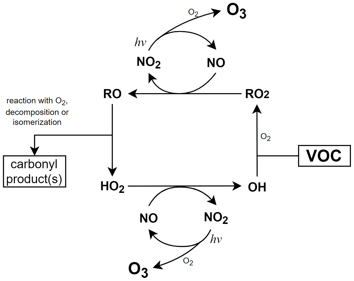
Figure 1The photochemical formation of O3 in the presence of NOx and VOCs (Jenkin and Hayman, 1999).
Wildfires emit large amounts of primary pollutants, like black carbon (BC), carbon monoxide (CO), NOx, and VOCs. Studies of boreal fire emissions show that the NOx concentrations can be doubled, and BC increased by 10 times when influenced by wildfires, even 1–2 weeks downwind in the middle of the Atlantic Ocean (Val Martín et al., 2006). The wildfire impacts on O3 production is a complex process involving various factors, such as fire precursor emissions, altered photochemical reactions, the effect on radiation by aerosols from the smoke plume, and local and downwind meteorological patterns (Jaffe and Wigder, 2012). Previous studies indicate that both NOx and VOCs emissions from wildfires influence the O3 budgets downwind, with enhancements ranging from 5 to 20 ppb (Baylon et al., 2015; Buysse et al., 2019; Jaffe and Wigder, 2012; McClure et al., 2018; Ninneman et al., 2021; Selimovic et al., 2020; Val Martín et al., 2006). When wildfire smoke reaches urban regions, the NOx, and VOCs in the smoke is believed to enhance O3 production (Akagi et al., 2013; Singh et al., 2012) and exacerbate the already problematic O3 pollution levels in many urban areas. Brey and Fischer (2016) found that the mean O3 abundance measured on smoke-impacted days is higher than on smoke-free days and the magnitude varies by location with a range of 3–36 ppbv. Furthermore, they found that the smoke-impacted O3 mixing ratios are most elevated in locations with the highest emissions of NOx.
However, the O3 response can vary from significant to small enhancements and even depletion during different wildfire events (Val Martín et al., 2006). Buysse et al. (2019) and McClure and Jaffe (2018) also report that maximum daily 8 h averaged (MDA8) O3 tends to decrease during heavy smoke influenced periods when PM2.5 (particulate matter with diameters that are smaller than 2.5 µm) exceeds 70 µg m−3. The reasons for this are not fully understood but may be explained by some of the following conjectures in the literature. Alvarado et al. (2010) found that on average 40 % of the NOx was converted to peroxyacetyl nitrate (PAN) within 1–2 h after emission, thus limiting NOx availability and in situ O3 production. The potential loss of O3 due to reaction with organic carbon could decrease O3 concentrations in wildfire plumes. For example, de Gouw and Lovejoy (1998) found that heterogeneous reaction between O3 and organic aerosol can be an important loss for tropospheric O3, particularly if the aerosols contain unsaturated organic material. Fischer et al. (2010) found O3 enhancements of about 20 ppb at a site downwind of a wildfire and estimated that about 8 ppb could be attributed to the decomposition of PAN during adiabatic warming during subsidence. Moreover, Buysee et al. (2019) found lower NO NO2 ratios when sites are influenced by wildfire smoke and suggested several potential reasons including elevated atmospheric oxidants (O3, RO2 and HO2), higher temperature, lower rates of NO2 photolysis due to shading, and increased interference in the NO2 measurements by other nitrogen species present in the wildfire smoke. A recent modeling study investigating a 2013 California wildfire showed that the simulation of near-fire smoke plume transport appears to perform well compared with satellite and aircraft measurements (Baker et al., 2018). While the photolysis rates in that study were also found to be well characterized by the model, the predicted O3, on the other hand, did not compare well with either surface site nor aircraft measurements: O3 was overestimated by the model both aloft and at the surface during periods impacted by wildfires anywhere from 5 to over 50 ppb.
As alluded to already, the vast amounts of absorbing aerosols like brown and black carbon emitted from biomass burning could also influence the amount of radiation that reaches the surface. Airborne studies using aerosol and radiation measurements indicate that a layer of high aerosol loading lying below a temperature inversion could drastically reduce the downwelling solar and UV irradiance, including the surface j(NO2) (Wendisch et al., 1996). Baylon et al. (2018) conducted an investigation of wildfire impacts on O3 production at a high elevation site located on Mt. Bachelor in Oregon and report j(NO2) decreasing by 14 %–21 % at high solar zenith angles when biomass burning plumes were detected, but slightly increasing (0.2 %–1.8 %) at local noon. Furthermore, meteorological factors that may be correlated with wildfires and the conditions that lead to their proliferation, such as temperature and humidity, could potentially affect the reactions associated with O3 production (Lin et al., 2017; Zhang et al., 2014). One study of the temperature dependence of O3 production in the San Joaquin Valley (SJV) (Pusede et al., 2014), for instance, found that the reactivity of total VOCs with OH (s−1) and the HOx production rate (PHOx ppts−1) both increased exponentially with temperature, leading to higher midday O3 concentrations by 1.5–2.0 ppb K−1. Steiner et al. (2010) also reported similar temperature dependencies on maximum 1 h ozone levels while underscoring their decreasing trend over the 25 years of their study, assumed to be a consequence of reducing NOx and VOC emissions across the state.
In the USA, the current National Ambient Air Quality Standards (NAAQS) for ozone is an MDA8 value equal to or exceeding 70 ppb. According to the California Air Resource Board (CARB), O3 concentrations frequently exceed existing health-protective standards in metropolitan areas of California during summer. In addition, the southern part of California's Central Valley (CV), the San Joaquin Valley (SJV), is still one of the two extreme O3 nonattainment areas remaining in the USA (U.S. EPA Green Book, https://www.epa.gov/green-book, last access: 3 February 2022). With the projection of an increasing likelihood of large wildfires in the future across the western USA (Brey et al., 2021; Stavros et al., 2014), it is important to understand how O3 production will change subject to the rising influence of wildfire events in the CV, and it will also be useful for the regulator to predict air quality degradation in the case of wildfire events.
In addition to the impacts of wildfires on air quality, Pahlow et al. (2005) present a proposed phenomenon that the shading effect of wildfire smoke can reduce the solar heating of the ground and lead to a shallower ABL, but the data evinced were only for 3 consecutive days on the US east coast. That study raises the question of whether the attenuation of ABL height due to wildfire shading is a general phenomenon and might it be supported by long-term observations. The strong correlation between downwelling surface solar radiation and ABL height has been described by previous studies. Pal and Haeffelin (2015) implemented a 5-year observational study of ABL height and surface fluxes near Paris in which they found the strongest determinant (r=0.92) of daily maximum ABL height was maximum downwelling shortwave radiation at the surface (SSWD), even more so than the surface heat flux (r=0.5). The strong correlation between SSWD and afternoon ABL height was also verified by Trousdell et al. (2016) in the SJV with a similar dependence of 1.5–1.7 mW−1 m2. The lowest portion of the free troposphere (FT) in the SJV has a complex structure with a “buffer layer” residing between ABL and FT, which is a layer of relatively stagnant air at altitudes between 500 to 2500 m resulting from the onshore wind that impinges on the southern Sierra Nevada mountains on the east side of the SJV (Faloona et al., 2020). This “buffer layer” accumulates the pollutants from the ABL by anabatic sidewall venting during the day but continuously returns some of the air via midday entrainment, with turbulence within the ABL being the key factor that controls the entrainment process. If the shading effect of wildfire smoke can considerably influence the ABL dynamics or ABL height, then it will be important to quantify the amount of ABL height attenuation that results from wildfire smoke and elucidate the impacts on the ventilation of pollutants in the SJV because entrainment has a direct impact on surface level concentrations of most pollutants (Trousdell et al., 2019).
In this paper, we use data from 10 CARB monitoring sites in the CV to quantify the impacts of wildfire smoke during summer (June–September) from 2016 to 2020. Then we use measured O3, NO, and NO2 (corrected approximately for known interferences) in a modified Leighton relationship (Volz-Thomas et al., 2003) to estimate changes to the O3 production rate P(O3), accounting for the observed shading effect of the wildfire smoke on j(NO2), as well as variations in ambient O3, and (rate constant in Reaction R2) due to temperature variations. In this way we are able to identify the specific impacts of wildfire emissions on regional ozone chemistry, whereas past studies have tended to leave these impacts mingled together. We also present the enhancement ratios (ERs) for O3 T, PM2.5 CO, and O3 production efficiency (OPE) during the wildfire-influenced periods in the CV. Then, we discuss the influences of wildfire smoke on surface buoyancy and heat fluxes (, QH, and QE) measured by two AmeriFlux monitoring sites located in the northern part of the SJV. We also use a radio acoustic sounding system (RASS, NOAA's Physical Sciences Laboratory, https://psl.noaa.gov/data/obs/datadisplay, last access: 17 November 2020, NOAA, 2020a) located near Visalia to study wildfire impacts on temperature profiles and ABL heights. Our study aims at using long-term observation data to quantify the differences of O3 concentrations and production rates during the wildfire-influenced periods in the CV and providing insights into the alteration of ABL dynamics that occurs in the presence of wildfire smoke.
2.1 Measurements
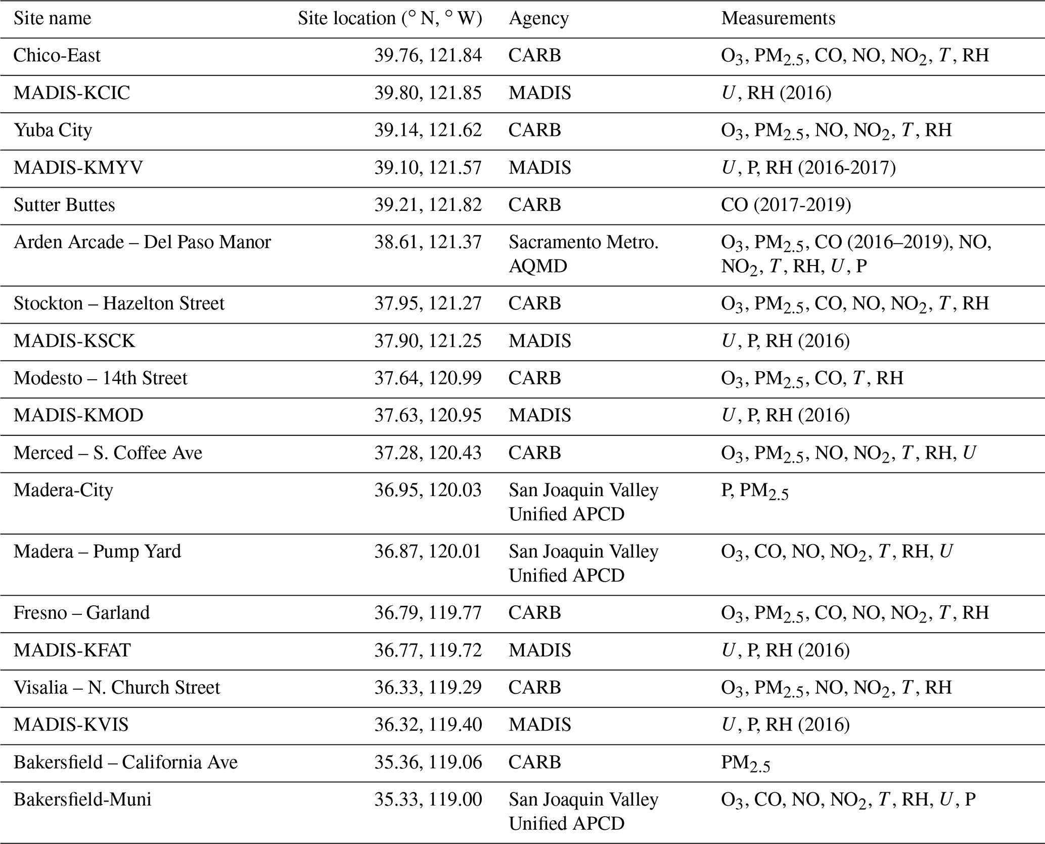
Measurements of hourly PM2.5, O3, nitric oxide (NO), nitrogen dioxide (NO2), and CO are taken from 10 CARB monitoring sites in the CV. Meteorological data, such as temperature, dew point, and pressure, are supplemented when needed from airports nearest each air pollution monitoring site. Figure 2 shows a map (© Google Earth 2020) of the locations of CARB sites as well as the RASS site and AmeriFlux sites used in our study. The locations and other detailed information about the sites can be found in Table 1. All the air pollution and meteorological data were downloaded via the CARB website (https://www.arb.ca.gov/aqmis2/aqmis2.php, last access: 17 February 2022), except for the data on reactive nitrogen compounds (NOy), which was downloaded via AirNow-Tech (http://www.airnowtech.org, last access: 17 February 2022). The CARB gather air quality data for the State of California and ensure the quality of these data, designs, and implemented air models, and sets ambient air quality standards for the state. The standard operating procedures for ambient air monitoring can be found on the CARB website (https://ww2.arb.ca.gov/resources/documents/standard-operating-procedures-ambient-air-monitoring, last access: 17 February 2022). The hourly-averaged data start at the beginning of the reported time. Singular missing hourly measurements are replaced by the average of the hour before and after; otherwise, missing data are disregarded. We found that 1.9 % of the 24 h PM2.5 and 1.5 % of the MDA8 O3 data are not available due to missing or erroneous values. We use temperature and relative humidity data from the CARB monitoring sites if they are available; otherwise, we use measurements from meteorological sites at the nearest airport (downloaded via AirNow-Tech, provided by Meteorological Assimilation Data Ingest system https://madis-data.ncep.noaa.gov, last access: 3 June 2021 (i.e., MADIS). Since relative humidity is a function that strongly depends on temperature, we also calculate specific humidity (q) from pressure measurements at the airport and the Clausius–Clapeyron relationship to eliminate the direct dependence on temperature. Because approximately 80 % of O3 exceedance days in the SJV typically occur between 1 June and 30 September (Trousdell et al., 2019), we focus on this period for each year (2016–2020). We calculate 24 h PM2.5 and MDA8 O3 as daily metrics, and the average of other pollutant concentrations are from 10:00 and 15:00 Pacific standard time (PST) as daytime averages that are most relevant to peak ozone levels.
The conventional measurement of NO2 entails the catalytic conversion of NO2 to NO on a heated molybdenum (Mo) surface and subsequently measured by chemiluminescence after reaction with O3. The drawback of this method is that other oxidized nitrogen compounds, such as PAN and HNO3, can also be converted to NO; thus, the molybdenum conversion method is known to cause overestimation of NO2. Steinbacher et al. (2007) proposed a correction method for overestimated NO2 measurements based on their long-term observations in rural Switzerland via Eq. (1):
where ΔNO2 is the amount of overestimation for NO2, is the measured NO2 concentration, O3 is measured ozone concentration; a, b, c, d, e, and f(month) are constants and f(day) is a binary predictor distinguishing day and night (1 or 0), and ε is a residual noise term that we ignored in our study. Details about those constants can be found in Table C1 in Appendix C. The NO2 at the Sacramento site is measured using a photolytic converter, which should not be affected by the interference from other oxidized nitrogen compounds to a large degree. All the NO2 measurements, except for those from the Sacramento site in this study, are corrected for according to Eq. (1), with the resultant NO2 decreasing on average by about 1.3 ppb (∼ 30 %) after the correction. This is not meant to perfectly eliminate all of the potential interferences in this measurement but is intended to eliminate the bulk of the interferences that are known to exist with this analytical technique. A similar analysis of the interference in the heated Mo technique, relative to a spectral NO2 measurement, was reported by Dunlea et al. (2007) in Mexico City, a very different environment, in which they found the long-term average to be ∼ 22 % in excess. Furthermore, the suburban sites reported in Xu et al. (2013) showed corrections also in line with what we used in this study, which are midday summer values of 25 %–40 %. In general, it is found that the Mo-chemiluminescence interference is proportionally smallest in urban regions, moderate in suburban regions, and highest in remote regions. We believe that the Central Valley of California is somewhere between urban and suburban/rural in its air quality, and therefore the Steinbacher et al. (2007) correction we use from their urban/rural site is reasonably appropriate in order to remove the first-order complications of this widespread chemiluminescence measurement. In Sect. 3.2 we investigate the uncertainty that is introduced into our estimation of the P(O3) due to errors in measurements in NO2.
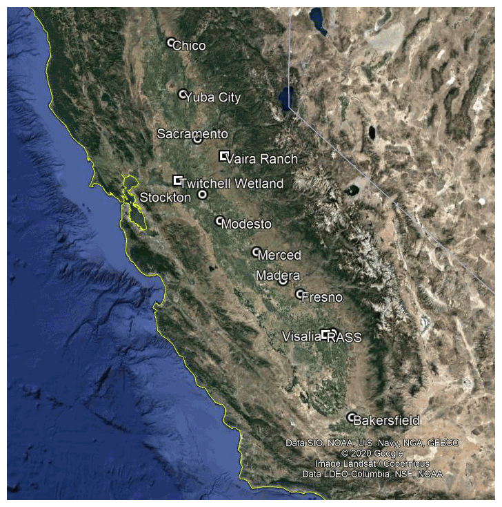
Figure 2A map of the locations of CARB sites (circles), the RASS site, and AmeriFlux sites (squares) used in this study (© Google Earth 2020).
Table 1The locations of measurement sites and detailed information.
2.2 Wildfire identification
We use the NOAA Hazard Mapping System (HMS, https://www.ospo.noaa.gov/Products/land/hms.html, last access: 11 December 2020) Fire and Smoke Product and the Hybrid Single Particle Lagrangian Integrated Trajectory (HYSPLIT) model accessed from AirNow-Tech (https://www.airnowtech.org/index.cfm, last access: 17 February 2022) as an identification tool for wildfire events. The HMS is an interactive environmental satellite image display and graphical system that was developed by the National Environmental Satellite, Data, and Information Service. The HMS is used by trained satellite analysts to generate a daily operational list of fire locations and outline areas of smoke (Brey et al., 2018). The analysts also rely primarily on visible satellite images to confirm that the fire locations are actually producing smoke. Then these detected points of fire locations are used to initiate the HYSPLIT model by NOAA, which is a complete system for computing simple air parcel trajectories, as well as complex transport, dispersion, chemical transformation, and deposition simulations (Stein et al., 2015), to estimate the movement of smoke in the National Weather Service (NWS) smoke forecast (Rolph et al., 2009; Ruminski et al., 2006). The HMS creates a fresh map for North America daily around 07:00–08:00 eastern standard time. For the performance time of the HMS in the CV (04:00–05:00 PST), this may cause a situation wherein the site is not detected by HMS with overhead smoke early in the morning but could be covered by smoke the rest of the day. In addition, because the HMS system is a satellite-based product, it is observed from above; therefore, it cannot differentiate surface wildfire plumes from lofted plumes and may also be limited by any cloud cover. These limitations may cause improper identification of wildfire events; therefore, we use additional methods to verify the presence of wildfire smoke at the surface level. Thus, we also use the HYSPLIT model to analyze the back-trajectories of the air parcels starting at each target site and trace its origin at surface level and within the ABL. By using the HMS and HYSPLIT, the steps for wildfire identification are as follows: first, we use the HMS product to see if any sites are covered by smoke. The target sites that are covered by the HMS smoke are marked according to the category of the HMS product as thin, medium, and thick smoke coverage. Second, we use the HYSPLIT model to calculate 24 h back-trajectories at 12:00 PST starting from the sites that are covered with the HMS wildfire smoke areas. The HYSPLIT model is performed at altitudes of 100, 600, and 1500 m, respectively, with a resolution of 12 km (NAM 12 km), which will provide the transport pattern near the surface, the top of the boundary layer, and in the middle of the “buffer layer” (Faloona et al., 2020) or what is sometimes called the “stable core layer” (Leukauf et al., 2016) of a valley atmosphere. Given that the low-level flow in the CV has a well-characterized diurnal pattern during summer (Zhong et al., 2004), we think that the HYSPLIT back-trajectory performed at three different levels are enough to represent the transport pattern of the air flow near the surface during our periods of study. If the HMS shows overhead smoke coverage and one of the HYSPLIT back-trajectories originated from, or passed by, the area of fire spots detected by the HMS, we define the target site as influenced by wildfire smoke on that day. The purpose of our method involving both the HMS and the HYSPLIT model is to identify cases that contain a significant impact of wildfire smoke at the surface level as accurately as possible. We believe that even if the fire plume is overhead and the back-trajectory ends above the ABL, strong daytime subsidence and entrainment over the valley will likely bring the wildfire effluent into the ABL and affect surface concentrations of air pollutants. Moreover, we also need a baseline to provide the conditions (e.g., pollutant concentrations, ABL height) without the influences of wildfire smoke to use as a control sample. We use images from the true color reflectance of MODIS Aqua and Terra to identify the days that are without cloud coverage and immediately before and after the wildfire-influenced periods as our baseline. In the following paragraphs, we will refer to those as the background or non-fire days. In this way, we are able to identify the wildfire events at each site and then use the baseline from background days to compare with the cases when the wildfire smoke is present at surface level.
2.3 O3 production
The modified Leighton relationship is a method to determine the relative magnitude of the in situ photochemical O3 production rate by measuring the extent to which the O3–NOx cycle is away from the photostationary state. This method represents the photochemical cycle of O3, NOx, HO2, and RO2 (Leighton, 1961). The chemical reactions entailed in this cycle are in Reactions (R1)–(R4), where j(NO2) is the photolysis rate in Reaction (R1), and , , and are reaction rate coefficients for Reactions (R2), (R3), and (R4), respectively. The role of wildfire smoke will include the addition of NOx and VOCs, which results in changing the concentration of HO2 , RO2, NOx, and their ensuing effects on O3 production:
The O3 production rate is derived from the modified Leighton relationship presented in Eq. (2). Reactions (R3) and (R4) determine the limiting rates for O3 production; thus, the production rate of NO2 in Reactions (R3) and (R4) is the effective production rate for “new” O3 that does not belong to the instantaneous photostationary state cycle. This can be expressed as:
where [NO], [NO2], and [O3] are hourly-averaged mixing ratios measured by CARB, and represent the contributions of VOC (and CO) in O3 production. The direct measurements of j(NO2) at ground level are not often available in field studies. Trebs et al. (2009) reported a relationship that can be used to estimate ground level j(NO2) directly from the solar irradiance, which is measured as a standard parameter in most field measurements. In the absence of direct measurement of j(NO2), this method is more reliable than radiative transfer calculations with poorly known input parameters. We use surface solar radiation measurements from the California Irrigation Management Information System (CIMIS, https://cimis.water.ca.gov/WSNReportCriteria.aspx, last access: 17 February 2022) to calculate the hourly j(NO2) by using a second-order polynomial function (Eq. A1) in Trebs et al. (2009) study. This approach is employed to account for the decreased photolysis rates during wildfire events due to the shading effect of the overhead smoke. Moreover, is also adjusted to corresponding hourly-averaged temperature measured at each site to account for the changes in rate coefficients due to temperature change using Eq. (A2) (Lippmann et al., 1980).
2.4 Boundary layer dynamics
We use surface eddy covariance flux data from two AmeriFlux sites located at Twitchell Wetland (Knox et al., 2018) (38.1074∘ N, 121.6469∘ W, −5 m) and Vaira Ranch (Ma et al., 2021) (38.4133∘ N, 120.9507∘ W, 129 m). The Twitchell site, which is located at a 7.4 acre restored wetland on Twitchell Island, has a flux tower equipped to analyze energy, H2O, CO2, and CH4 fluxes since May 2012. The wetland is almost completely covered by cattails and tules by the third growing season. Vaira Ranch site has been established at the lower foothills of the Sierra Nevada on privately owned land since 2000; the site is classified as a grassland dominated by C3 annual grasses. The measurements at the two sites include surface sensible heat flux (QH), latent heat flux (QE), temperature, incoming shortwave radiation, and the mole fraction of water vapor. The time resolution is 30 min, and the measurements are available from 2016 to 2019. The surface buoyancy flux is calculated by Eq. (4), where , , and are direct measurements from the site, and is calculated from the measured mole fraction of water vapor:
We use the same wildfire events identification results from Sect. 2.2 to categorize wildfire days and background days, where Twitchell Island (30 km northwest of Stockton) uses the results of Stockton and Vaira Ranch (50 km southeast of Sacramento) uses the result of Sacramento. Then, we calculate the averaged diurnal profile for , QH, QE, and incoming shortwave radiation for wildfire-influenced and background days at each site.
Radio acoustic sounding systems (RASS) remotely measure the virtual temperature and wind profile up to about 2 km, and their 1 h time resolution has substantial advantages over radiosondes. We use the virtual temperature data measured by the RASS located near the Visalia Municipal Airport. Then, the virtual temperature is converted into virtual potential temperature by the hypsometric and Poisson's equations based on the surface measurements of temperature and pressure. The ABL height is estimated by the first range gate where the vertical virtual potential temperature gradient exceeds 10 K km−1. Then, the estimated ABL heights are also sorted into wildfire-influenced days and background days for comparison. A 5-year monthly averaged diurnal ABL height profile retrieved by this method during June–September from 2016 to 2020 is shown in Fig. B4 in Appendix B. The magnitude and timing of the ABL heights correspond approximately to the diurnal ABL profiles in the SJV measured by Bianco et al. (2011) and Faloona et al. (2020).
3.1 Summary of wildfire events from 2016 to 2020
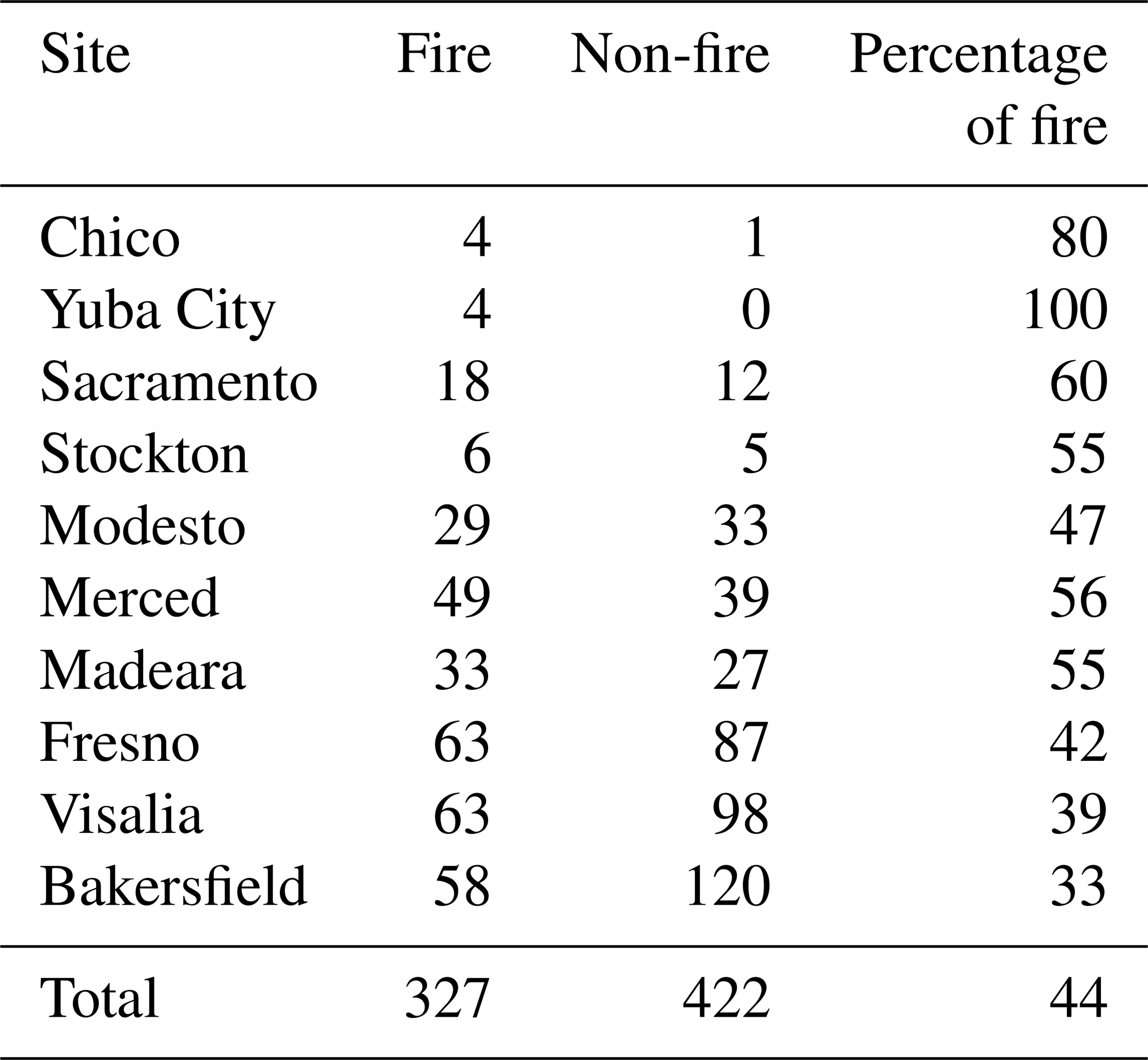
During the summer (June–September) in the CV, wildfires are prone to happen amidst the mountains that surround the valley and spread upslope in general. The yearly acres burned by wildfire in California during the study ranges from 259 148 in 2019 to 1 823 153 in 2018 (National Interagency Coordination Center, https://www.nifc.gov/fireInfo/fireInfo_statistics.html, last access: 11 December 2020). By September 2020, the 2020 fire season in California had become the most intense year of the 18-year fire radiative power measurements collected by satellite (NOAA/NESDIS Hazard Mapping System, https://www.ospo.noaa.gov/Products/land/hms.html, last access: 11 December 2020). The number of wildfire-influenced days at each site are presented in Table C2. Although the wildfire-influenced days vary from site to site, the average total number of the wildfire days are about 120 d out of 600 d (∼ 20 %) from our 5-year data analysis (2016–2020). The composite means of the 500 hPa geopotential height fields are shown in Fig. B5 indicating that the climatological coastal trough is more dominant during the background days, and the high-pressure bulge of the warm southwestern US lower troposphere is more dominant across California during wildfire days leading to higher temperatures and less synoptic ventilation.
We summarize the characteristic value of daily maximum temperature (Tmax), relative humidity (RH), specific humidity (q), scalar-mean windspeed (U), 24 h PM2.5, MDA8 O3, CO, and NOx for wildfire and background days at each site in Fig. 3. The error bars show the interquartile range limited by the 25th and 75th percentiles, and the center mark denotes the median value. For 24 h PM2.5 and CO, concentrations on wildfire days are significantly higher than non-fire days at all sites, since fine particles and CO are major products of biomass burning and are also good tracers of wildfire smoke. On average, the 24 h PM2.5 and CO are 8.7 µg m−3 (∼ 102 %) and 76 ppb (∼ 48 %) higher than background periods, respectively. For most sites, the 25th percentile of the wildfire value is higher than the 75th percentile of non-fire periods. The clear difference in the concentrations of PM2.5 and CO between wildfire and background days suggest that our wildfire identification method using the HMS in conjunction with the HYSPLIT back-trajectory model can appropriately detect the presence of wildfire smoke at surface levels. It also suggests that our identification method has a similar effectiveness compared with methods that use the HMS and background PM2.5 or CO as a threshold (e.g., mean background values plus one standard deviation) for wildfire identification in previous studies (McClure et al., 2018; Briggs et al., 2016). The MDA8 O3 and NOx concentrations are also enhanced during fire days by 6.5 ppb (∼ 12 %) and 0.9 (∼ 32 %) on average. The histograms in Fig. B1 show that about 9 % and 40 % of the wildfire-influenced days exceed the NAAQS of 70 ppb MDA8 O3 vs. only 3 % and 16 % during background periods for SV and SJV, respectively. The numbers and percentages of MDA8 O3 exceedances of 70 ppb at each site are presented in Table C4. Overall, the wildfire events contribute to about 44 % of the total exceedance cases. Using a global chemical transport model Pfister et al. (2008) estimated that the MDA8 O3 increased by about 10 ppb on average for all sites in California during the wildfire events in the fall (September–December) of 2007. Note that our study focuses only on the CV region in the summer months a decade later when the ambient NO2 levels have decreased by approximately 50 % in large urban areas (Simon et al., 2015) in California, and the model of Pfister et al. (2008) exhibits biases in MDA8 O3 of 10–15 ppb in fire and background conditions. Moreover, Fig. 3 shows that the MDA8 O3 has a southward directed gradient, in general, with higher O3 concentration in the SJV than in the SV independent of whether or not wildfire emissions are present. This result is consistent with the EPA Green Book and the study conducted by Trousdell et al. (2019), in which they find that O3 pollution in the SJV is still a problem.
For meteorological factors, all sites except Chico show a higher median value (∼ 0.5 K on average) of Tmax on wildfire-influenced days. The result of higher temperature matches the previous long-term climatology studies on wildfire in the USA from 1971 through 1984 (Potter, 1996), in which they report that wildfire events correspond to positive temperature anomalies. Brey et al. (2018) also show that in Mediterranean California, the temperature is positively correlated with human-ignited burn area and the precipitation and RH are negatively correlated with both, the human-ignited and lightning-ignited areas, though the Pearson correlations are relatively smaller in California than in other regions. The study of Brey et al. (2021) found that in California's mountain regions, using wind speed, RH, and vapor pressure deficit (VPD) as the predictors of wildfire, burn areas yield ubiquitously small coefficients, and that only when RH is excluded as a predictor does the coefficient for summer VPD become appreciable in both historical data and future projections. However, in our study, a consistently higher specific humidity (q) is observed at all sites during wildfire periods by 0.6 g kg−1 on average. Additionally, higher RH values are also detected at most sites except for Merced and Bakersfield. The higher water vapor content observed in the valley ABL during wildfire periods is most likely not attributable to the chemical product of fuel combustion in the wildfires because that contribution would be stoichiometrically similar to CO2 which is only observed to be enhanced by about ∼ 10 ppmv in such environments (Langford et al., 2020). Furthermore, the surface wind speeds show a reduction of about 0.3 m s−1 on average during wildfire periods at most sites except for Madera and Fresno. Thus, we hypothesize that the higher water vapor content and lower wind speeds are the result of weaker ABL entrainment due to the shading effect from wildfire plumes because of the reduced surface heat fluxes. This will be discussed further in Sect. 3.3.
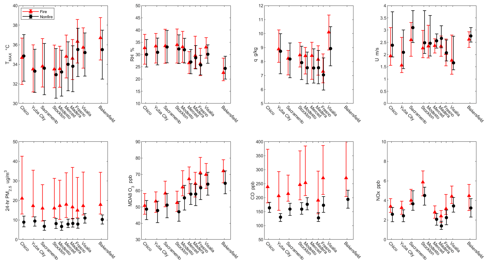
Figure 3Median values for fire (red triangles) and non-fire (black circles) periods at each station; error bars represent 25th and 75th percentile values. RH, q, U, CO, and NOx are 5 h averaged values between 10:00 and 15:00 PST. The interval of station-axis labeling is scaled to the latitude of each site. The number of data points within each group of error bars are the same as the number of wildfire days and background days shown in Table C2, unless there are missing data.
We note that the O3 concentrations have a relatively strong correlation with ambient temperature (Fig. B2); thus, this meteorological variation needs to be considered when we analyze the O3 enhancement (i.e., enhancement ratios for O3 and temperature). According to Pusede et al. (2014), a study of daily maximum temperature vs. daytime (10:00–14:00 local time) O3 concentrations in Bakersfield, California, show the change of O3 concentration with respect to temperature variation (ΔO) to be around 2 ppb K−1. Steiner et al. (2010) report O3-temperature slopes of 2.4 and 1.8 ppb K−1 in SJV and SV, respectively, yet their data are already a decade old, and they found that these slopes had been decreasing over the 30 years of their study. Our study (Fig. B2) shows that ΔO is on average 1.7 ppb K−1 for the background periods in the SJV and 1.3 ppb K−1 in the SV, consistent with a continued decrease in this parameter over time. Moreover, we found that the average slopes increase in the presence of wildfire emissions to 2.2 (SJV) and 1.6 ppb K−1 (SV) also consistent with its dependence on precursor emissions (Sillman and Sampson, 1995). Thus, with an average of 0.5 K increase in temperature (Tmax), we expect that approximately 1 ppb of the observed O3 enhancement is due to the temperature increment during wildfire periods and the rest, 5.5 ppb of O3 enhancement, is due to the influences of wildfire smoke. We also found that the ERs for ΔPMCO have a strong positive correlation at all 10 sites (Fig. B3), indicating that the PM2.5 and CO are well connected to wildfire influence. Our average ER for ΔPMCO (m value in Fig. B3) is 0.12 (± 0.03) µg m−3 ppb−1, which agrees well with the value (0.107) found by Selimovic et al. (2019) in a study from two summers in Missoula, Montana, as well as the value (0.12) reported by McClure and Jaffe (2018) from wildfires in Idaho.
3.2 Wildfire smoke influences on PM and O3 production
In order to investigate the O3 variations and their relationship to the existence of additional PM from wildfire smoke, we plot the binned 24 h PM2.5 vs. corresponding MDA8 O3 in Fig. 4. Since O3 enhancements react differently across the CV, we separate our sites into two geographical categories: Chico, Yuba City, and Sacramento into Sacramento Valley (SV) (Fig. 4b); and the remaining sites to the south into the SJV (Fig. 4c). Generally, MDA8 O3 increases with PM at low 24 h PM2.5 concentrations for both the wildfire and background periods, peaking around 40–55 µg m−3, then becomes independent of PM at higher concentrations (PM2.5 > 55 µg m−3). The slopes of the O3 to PM2.5 relationship (below 40 µg m−3) are higher in the SJV than the SV. The non-linear relationship in our results generally aligns with the results from previous studies (Buysse et al., 2019; McClure et al., 2018) in which an increase in MDA8 O3 with PM is found at low to moderate PM with a peak of MDA8 O3 around 40–55 µg m−3. However, our results do not show a clear decreasing trend of MDA8 O3 at higher PM. The MDA8 O3 does slightly decrease when PM2.5 exceeds 55 µg m−3 in SJV, but it returns to its peak value when PM2.5 > 100 µg m−3.
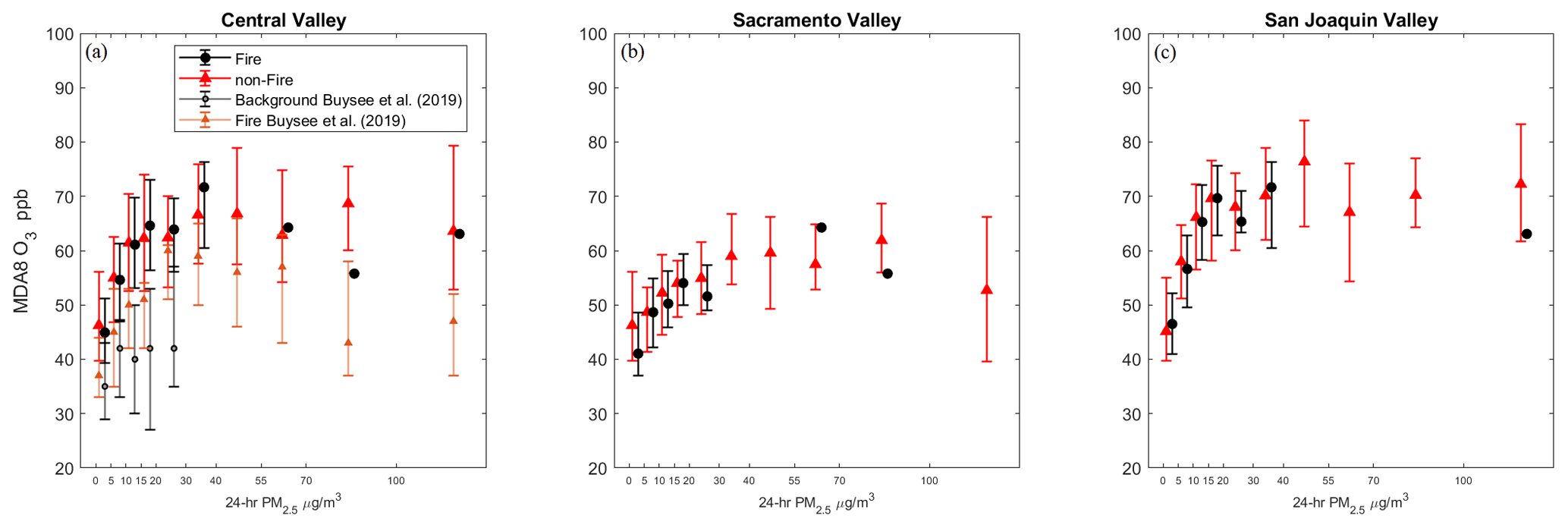
Figure 4Plots for binned 24 h PM2.5 vs. MDA8 O3 for all 10 sites (a). Chico, Yuba City, and Sacramento are in (b) and all other sites in the SJV in (c). Black dots and red triangles denote the median value for the background and wildfire periods, respectively. The error bars denote the 25th and 75th percentile values. The number of data points in each bin can be found in Table C3. The orange (fire) and gray (non-fire) error bars are the results reported by Buysee et al. (2019) for comparison.
The NO levels, estimates of O3 production rates (PO3), and their dependence on the NO2 correction, along with the attenuation of incoming solar radiation, are shown in Fig. 5. The peak value of solar radiation (Fig. 5d) decreases by 7 % on average at all 10 sites during the wildfire periods. The P(O3) (Fig. 5c) estimated from the modified Leighton ratio increases at all sites during the wildfire-influenced periods. Despite the diminution of j(NO2) due to the shading effect of wildfire smoke, and the general enhancements of NO and O3, the P(O3) increases by up to ∼ 50 % (derived as the ratio of the valley-wide P(O3) averages in wildfire vs. background conditions). The uncorrected, fully corrected, and 20 % intermediate stages of NO2 correction are illustrated in Fig. 5b in order to represent the sensitivity of P(O3) to our NO2 correction magnitude separated into background (black) and wildfire (red) data. On average, the P(O3) changes linearly by about 30 ppb h−1 for 1 ppb of NO2 correction, and there is no significant difference in slope between wildfire and background conditions (29.1 vs. 31.0). In the full correction, only one site, Bakersfield, shows a negative median value of P(O3) for background days, but the valley-wide average is 18.7 ppb h−1. We consider this a very noisy measurement, but some meaning can be retrieved in the valley-wide average. In order to contextualize these estimates, we present a summary of the midday P(O3) values that have been reported in the literature for the Southern San Joaquin Valley (SSJV) in Table 2.
Table 2A summary of reported midday ozone photochemical production rates in the southern SJV.
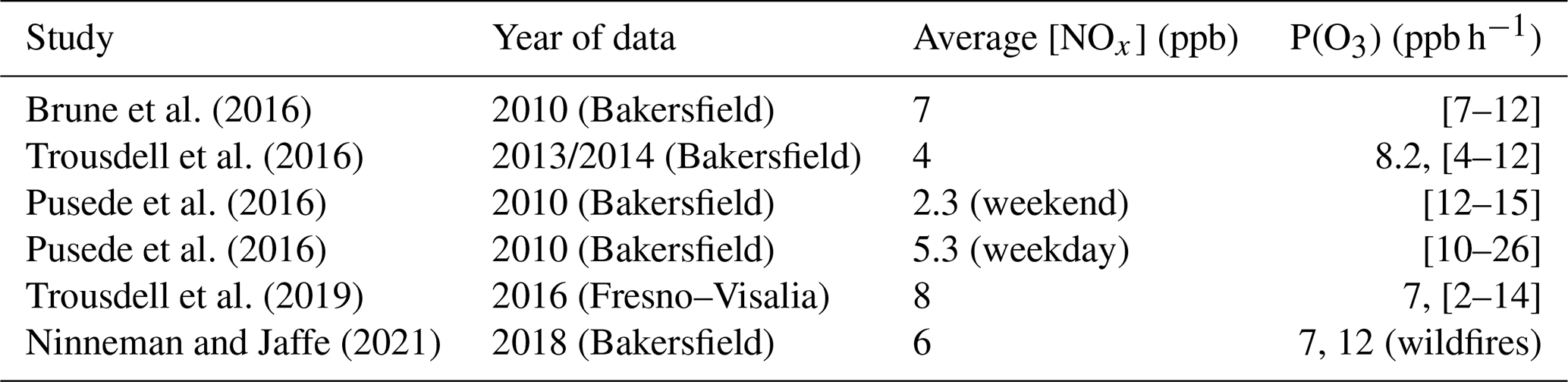
Note: Square brackets in the last column represent the interval of the P(O3) rate.
Realizing that this study found the average NOx to be only ∼ 3 ppb, and that the NO2 NO photostationary state method is known to overestimate P(O3) by about 2.5 times (Mannschreck et al., 2004), we can crudely surmise that the values we estimate should be in the range of about 10–20 ppb h−1, and thus the correction of Steinbacher et al. (2007) is most likely accurate to within ∼ 30 %. Furthermore, assuming that the NO2 corrections in the presence of fire smoke are most likely larger than those used here (from the average conditions of Steinbacher et al., 2007), we infer that the average influence of wildfires in the Central Valley is to enhance in situ ozone production rates by at most 50 % (18.7–28.3 ppb h−1) and consider this to be an upper limit of enhancement. Although we acknowledge the large uncertainty in this modified Leighton method, we do believe that the results are still instructive in analyzing the relative changes in P(O3) during wildfire and background periods indicating that despite the 7 % decrease in photolysis rates and enhancements in O3+ NO reaction rates, ozone production increases up to 50 % in wildfire conditions. Finally, any additional NOy interference that is not fully corrected for by the Steinbacher et al. (2007) formula is likely due to the presence of oxidized nitrogen species originating from the wildfires and thus has contributed to the ozone enhancement somewhere along its path from the fire to the urban monitoring site, even if it is not concurrently increasing the in situ photochemical production rate.
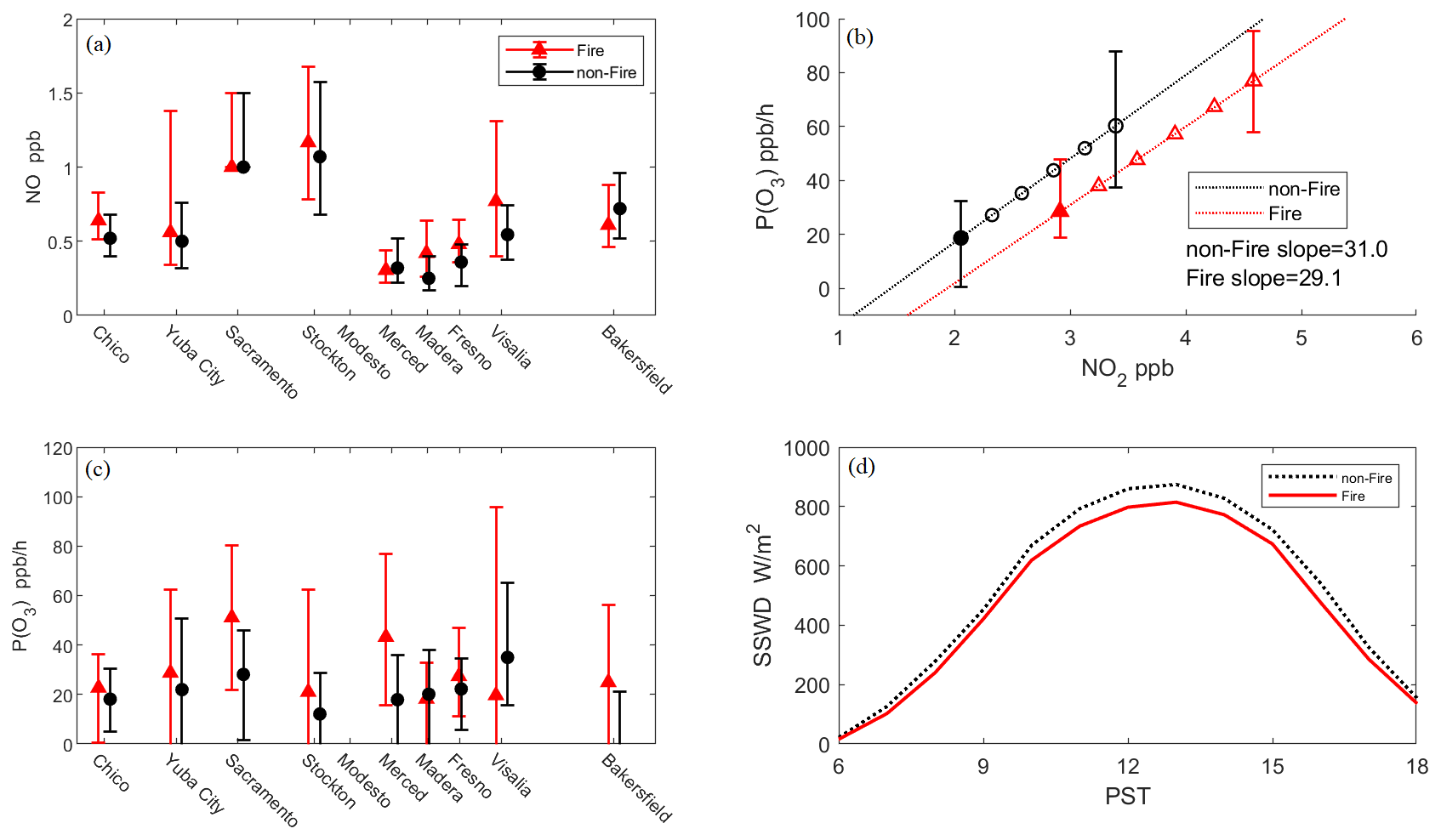
Figure 5Plots of (a) NO measurements, (b) calculated P(O3) (ppb h−1) at each stage of NO2 correction (0 %–20 %–40 %–60 %–80 %, open, and 100 %, solid), (c) calculated median PO3 at each site, and (d) averaged diurnal profiles for SSWD measurements. The error bars in (a), (b), and (c) represent the 25th and 75th percentiles for the 5 h averaged values between 10:00 and 15:00 PST during wildfire days (red) and background days (black).
O3 production efficiency (OPE) is defined as the enhancement of Ox (O3+ NO2) with respect to NOz (NOy–NOx). It describes the amount of O3 that is produced per NOx molecule consumed (Lin et al., 1988; Liu et al., 1987; Olszyna et al., 1994; Trainer et al., 1993). Figure 6 shows scatter plots for Ox vs. NOz in Fresno (SJV) during the 2016–2020 O3 seasons for both wildfire and background data. The slope value (m) is the enhancement of Ox with respect to NOz or OPE. Overall, the OPE does not show significant changes when impacted by wildfires. The OPE is known to monotonically decrease with increasing NOx and increase with VOCs under most conditions (Lin et al., 1988; Sillman, 1999). Thus, the insignificant changes in OPE indicate that the enhanced ozone level in SJV are likely due to the concomitant presence of additional VOCs ROx and NOx in approximately comparable measures.
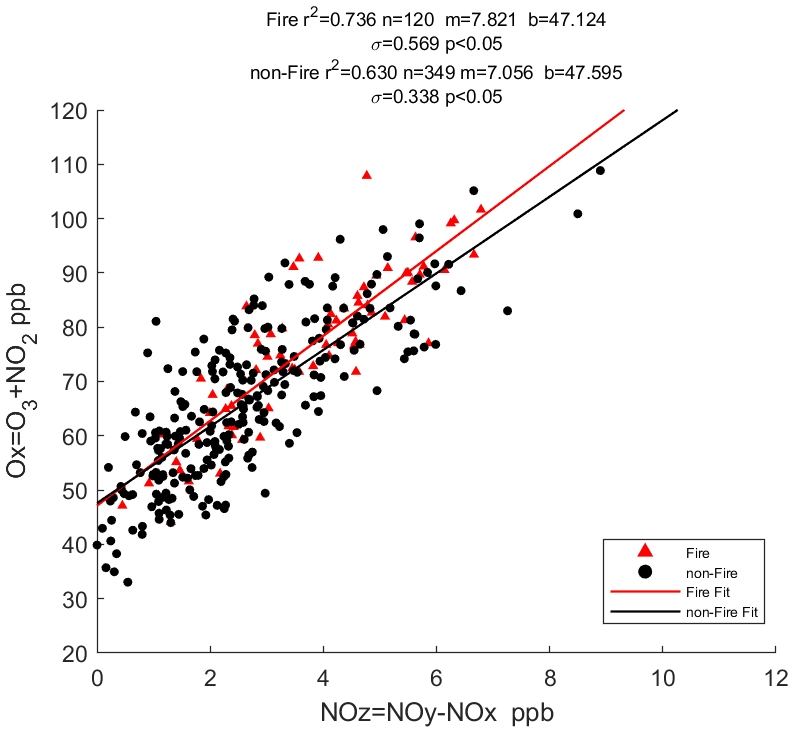
Figure 6Scatter plot of Ox vs. NOz at Fresno. The slope of the linear regression (m) represents the OPE; n is the number of data points in the scatter plot, σ is the standard error for the linear regression, and p is the P value that represents the rejection of the null hypothesis. In this case, the P values are less than 0.05, which we interpret as the regressions being statistically significant.
3.3 Wildfire smoke's influence on boundary layer dynamics
Measurements of surface heat fluxes (QH, QE, and ) and SSWD at Twitchell Wetland (bottom) and Vaira Ranch (top) are shown in Fig. 7. Both the sensible heat flux QH and buoyancy flux decrease during the wildfire periods, especially at Twitchell Wetland, where and QH are only about half as large on background days. The peak value of QE at Vaira Ranch decreases by 20 W m−2 but increases by 20 % on average at Twitchell Wetland. Note that, due to the difference in land types, the soil moisture is significantly higher in Twitchell than Varia, which explains the significantly smaller QE in Vaira Ranch compared with Twitchell Wetland with a Bowen ratio of 11.7 and 0.6, respectively. Furthermore, the augmented latent heat fluxes at Twitchell Wetland, despite the reduced SSWD during wildfire conditions, is consistent with an “oasis effect” observed at the site wherein horizontal advection of warmer/drier air enhances evapotranspiration (Baldocchi et al., 2016). Across all sites, the reduced SSWD , QH, and below wildfire plumes will weaken the turbulent mixing within the ABL, reducing the ABL growth rate and height, which in principle would enhance the specific humidity and weaken the surface wind speed because a reduced buoyancy source of turbulent kinetic energy (TKE) will reduce the entrainment fluxes of dry, higher momentum air across the inversion. Our results are consistent with the LES study of aerosol loading in the ABL by Liu et al. (2019), which showed that as aerosol optical depth (AOD) increases, less solar radiation reaches the surface, reducing the surface buoyancy flux and weakening the entrainment.
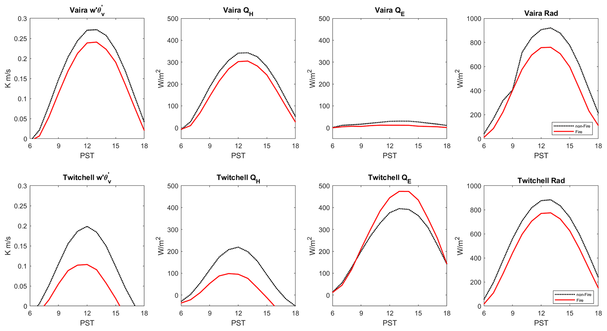
Figure 7Measurements of buoyancy flux (), sensible heat flux (QH), latent heat flux (QE), and incoming solar radiation (SSWD) at Vaira Ranch (top row) and Twitchell Wetland (bottom row). Solid red lines are averaged profiles during wildfire periods (June–September) from 2016 to 2019. Dashed black lines are the averaged profile for non-fire days.
In order to visualize the condition of a polluted ABL during wildfire-influenced periods, Fig. 8 presents the daily averaged aerosol backscatter profiles during wildfire days (a) and background days (b) observed during the California Baseline Ozone Transport Study (Faloona et al., 2020; Langford et al., 2020). The aerosol backscatter profiles are measured by a Tunable Optical Profiler for Aerosol and Ozone lidar (TOPAZ) that was located in Visalia, California. During the wildfire periods, the backscatter is seen to be much greater in and above the ABL compared with the background days. We also show the averaged afternoon (13:00–15:00 PST) vertical profiles of backscatter in Fig. 8c, where the aerosol load (i.e., backscatter β) is nearly doubled within the ABL (typically found up to ∼ 600 m) during wildfire days. Figure 9a shows the profiles of virtual potential temperature (θv) measured by the RASS located in Visalia. The profile is averaged from 13:00 to 15:00 PST during the summers of 2016–2020 for wildfire days (red) and background days (black) because daily maximum ABL height usually occurs around 14:00 in SJV (Bianco et al., 2011). The θv within the entire ABL is consistently about 1–2 K higher during wildfire days, and the warming is also apparent well above the ABL, which implies that aerosols within the lower valley atmosphere from wildfire plumes absorb solar radiation and warm the ABL and the buffer layer above it without appreciably influencing the stability per se. Liu et al. (2019) also simulate a warmer ABL with aerosols present in their LES and potential temperature increasing with AOD. While we cannot be certain that the warmer lower troposphere under wildfire influence is solely due to shortwave absorption, as opposed to simply climatological differences between wildfire and non-wildfire periods, we do know that surface SSWD and surface heat fluxes are reduced, so the enthalpy difference would likely be found in the lower troposphere. Assuming the 54 Wm−2 difference was fully absorbed in the lower 2 km of the valley atmosphere over the course of 8 h, this would lead to a heating of ∼ 0.8 K. Furthermore, a study by David et al. (2018) shows that over a 6-year period in northern California wildfire smoke systematically lowers the SSWD by about 120 Wm−2 and raises the surface air temperature by about 1 K for each increase in AOD of 1. The 5-year averaged diurnal ABL height comparison between wildfire periods and background days is shown in Fig. 9b with SSWD comparison shown in Fig. 9c. The midday ABL height is reduced by 80 m and the SSWD by about 54 W m−2 on average. Pal and Haeffelin (2015) reported the slope for SSWD vs. daily maximum ABL height to be 1.73 mW−1 m2 from an observatory outside of Paris, and Trousdell et al. (2016) reported a similar slope of 1.51 mW−1 m2 in the SJV. In this study, the observed reduction in ABL height and SSWD due to the wildfire shading effects shown in Fig. 9 (80 m/54 Wm−2 = 1.48 mW−1 m2) is quantitatively similar to the relationship between ABL height and SSWD in these other studies. It is also worth noting that the altitude of the highest backscatter gradient, which is another indicator of ABL height apart from the inversion of θv (Hennemuth et al., 2006), is actually lower during wildfire days (∼ 550 m) than on background days (∼ 650 m). The lowered backscatter inversion also illustrates that the ABL height is stunted due to the shading effect of the wildfire smoke plume. Since the wildfire plumes will weaken the entrainment at the ABL top and lower the ABL height, the rate of dilution from the buffer layer into the ABL and the volume for pollutant dispersion will also be reduced. Thus, the phenomenon of higher water content and lower wind speed described in Sect. 3.1 could also be the consequence of weaker turbulent mixing within the ABL and the lower ABL heights observed during the wildfire days.
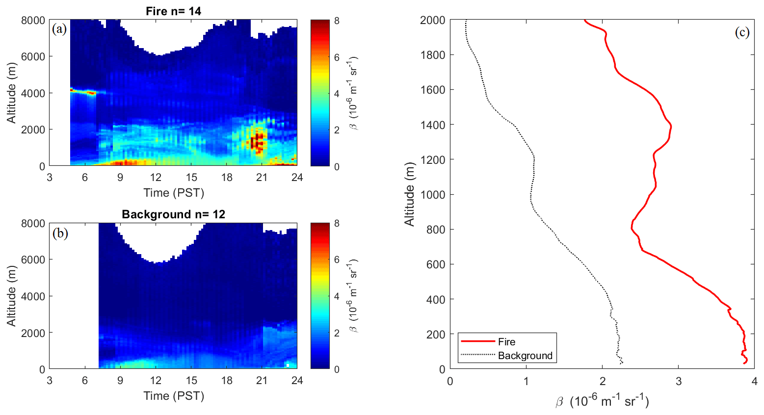
Figure 8Aerosol backscatter profile for TOPAZ during CABOTS 2016. The plots are the averaged diurnal profile for wildfire days (a) and background days (b) during 18 July to 7 August 2016. Averaged vertical backscatter profiles for wildfire days (red) and background days (black) between 13:00 and 15:00 PST are in (c). The n is the number of days in each plot. The TOPAZ produces a vertical profile for every 12 min with a resolution of 5 m.
Therefore, the wildfire smoke plays two distinct roles in influencing the ABL dynamics and scalar budgets. First, by attenuating surface insolation the smoke reduces the surface heat fluxes weakening ABL entrainment thereby decreasing the maximum ABL height, decreasing ABL wind speeds, and increasing water vapor mixing ratios. The weakened entrainment will likely affect other scalars, such as methane, N2O, and CO2, that are strongly influenced by entrainment dilution (Trousdell et al., 2019), all else being equal; however, these trace gases are likewise influenced by wildfire emissions, so the impacts are more complex. Second, the smoke absorbs solar radiation warming the air in the ABL (and above) thereby offsetting the reduced surface and entrainment heat fluxes in terms of its impact on air temperature.

Figure 9Averaged virtual potential temperature (θv) profile between 13:00 and 15:00 PST (a), diurnal profile for daytime ABL height (b), and diurnal SSWD profile (c) at Visalia during wildfire days (red) and background periods (black) from 2016 to 2020.
O3 pollution is still an issue in California's urban regions during summer seasons when wildfires are also prone to happen, and which are becoming larger and more frequent. The wildfires cannot only emit primary pollutants like CO, NOx, black carbon, volatile organic compounds, and fine particles, but also provide reactants for the production of secondary pollutants like O3. We used data from 10 sites in California's Central Valley region during the summers from 2016–2020 and identified wildfire events by the HMS and HYSPLIT modeling. On average, the wildfire-influenced days in the CV added up to about 20 % of the entire summer (∼ 120 d out of 600 d). During these periods we found that MDA8 O3 increases by 6.5 ppb on average with about 5.5 ppb (+10 %) being attributable to the wildfires after correcting for the bias in temperature for wildfire conditions. Furthermore, NOx concentrations during daytime increase by up to 0.9 ppb (∼ 32 %) and CO is higher on average by 76 ppb (48 %). The MDA8 O3 increases with 24 h PM2.5 at low to moderate concentrations, peaks at 40–55 µg m−3, and is more or less independent of PM2.5 at higher concentrations. From our 5-year data analysis, the probability of exceeding the NAAQS of 70 ppb MDA8 O3 is more than doubled (9 % and 40 %) during wildfire-influenced periods compared with background periods (3 % and16 %) for SV and SJV, respectively. The wildfire events contribute to about 44 % of the total exceedance cases. Daily maximum temperature and specific humidity show enhancement at most sites (averages of +0.5 K and +0.6 g kg−1), whereas midday windspeed is slightly decreased. The in situ P(O3) exhibits enhancement at all stages of NO2 correction, and by an average of up to ∼ 50 %, despite j(NO2) being reduced due to the shading effect of the wildfire plumes. The analysis indicates that P(O3) would change significantly with the uncertainties of NO2 measurement (∼ 30 ppb h−1 P(O3) ppb−1 NO2), which suggests that accurate measurements of NO2 are crucial to accurately estimating P(O3) by using the modified Leighton relationship. Nevertheless, our results still show distinctive differences of the P(O3) between wildfire and background periods, even with relatively large uncertainties in the NO2 measurements. The OPE has insignificant changes in the SJV despite the increase in NOx during wildfire influence from which we conclude that both the VOCs and their oxidation products, and NOx from wildfire plumes, contribute to increasing O3 production.
We analyzed surface heat flux measurements from two AmeriFlux sites located in the northern SJV and ABL temperature profiles and ABL heights from a RASS site near Visalia. We found that the surface buoyancy flux decreases by an average of 30 % when overhead wildfire plumes are detected. We also found that the midday ABL height decreases by 80 m on average with an attenuation of 54 W m−2 in SSWD. Despite the decreased surface buoyancy fluxes, the θv measurements from RASS show that the ABL becomes 1–2 K warmer on average during wildfire-influenced periods. This implies that the ABL dynamics will change due to the presence of wildfire plumes and are the net result of two factors: first, the shading effect of the wildfire plumes decreases the SSWD, surface heat fluxes, and consequently reduces the ABL height. Second, the additional aerosols in the ABL absorb solar radiation and warm the ABL as well as the “buffer layer” above it. Since the turbulent entrainment mixing into the ABL and the height itself have critical impacts on the concentration budgets of constituents (e.g., pollutants, water vapor), the weakened turbulent mixing and lowered ABL height will serve to make an already polluted ABL even worse.
The equation for j(NO2) calculation from surface solar radiation measurements (Trebs et al., 2009):
where and W−1 m2 s−1 are polynomial coefficients and G is solar radiation measurement.
Equation (A2) is the Arrhenius function to calculate based on temperature T, and the result derived from the function fits the experiment result extremely well through the common temperature range of 283–364 K (Lippmann et al., 1980).
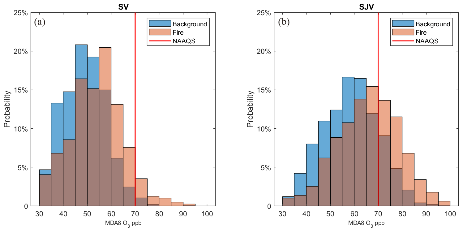
Figure B1Histograms of MDA8 O3 for wildfire periods (orange) overlaid on background periods (blue) during summer (June–September) from 2016 to 2020. The sites are sorted into SV (a) and SJV (b). During wildfire periods, about 9 % and 40 % of the days exceed the NAAQS of 70 ppb MDA8 O3 (red line) vs. only 3 % and 16 % during background periods for SV and SJV, respectively.

Figure B2Scatter plot and linear regression for daily maximum temperature vs. MDA8 O3 at each site for wildfire periods (red) and background periods (black). The R2 above each figure is the coefficient of determination, m is the slope or enhancement ratio, n is the number of data points in the regression, σ is the standard error for the linear regression, and p is the P value that represents the rejection of null hypothesis.
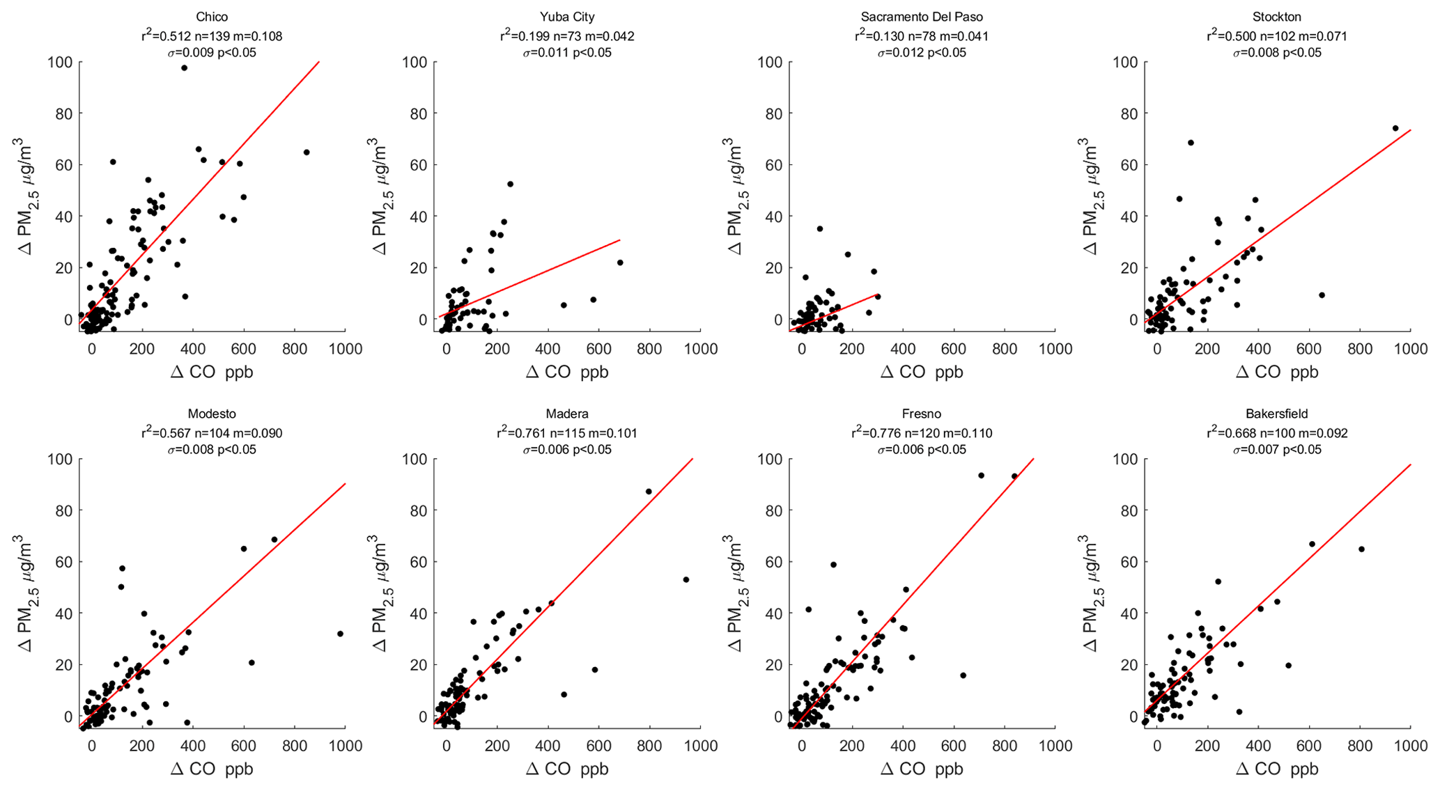
Figure B3Scatter plot and linear regression for ΔPM2.5 vs. ΔCO at each site. Enhancements are the differences in afternoon (10:00–15:00 PST) mean values between wildfire and background periods. The m is the slope or enhancement ratio, n is the number of data points in the regression, σ is the standard error for the linear regression, and p is the P value which represents the rejection of null hypothesis.


Figure B5The composite means of 500 mb geopotential height for wildfire days (left) and background days (right) during summer 2016–2020 (NOAA Physical Sciences Laboratory, https://psl.noaa.gov/cgi-bin/data/getpage.pl, last access: 20 April 2022).
Table C1Constants in Eq. (1) for NO2 correction (Steinbacher et al., 2007). The result is from the multiple linear regression model at the Taenikon site.
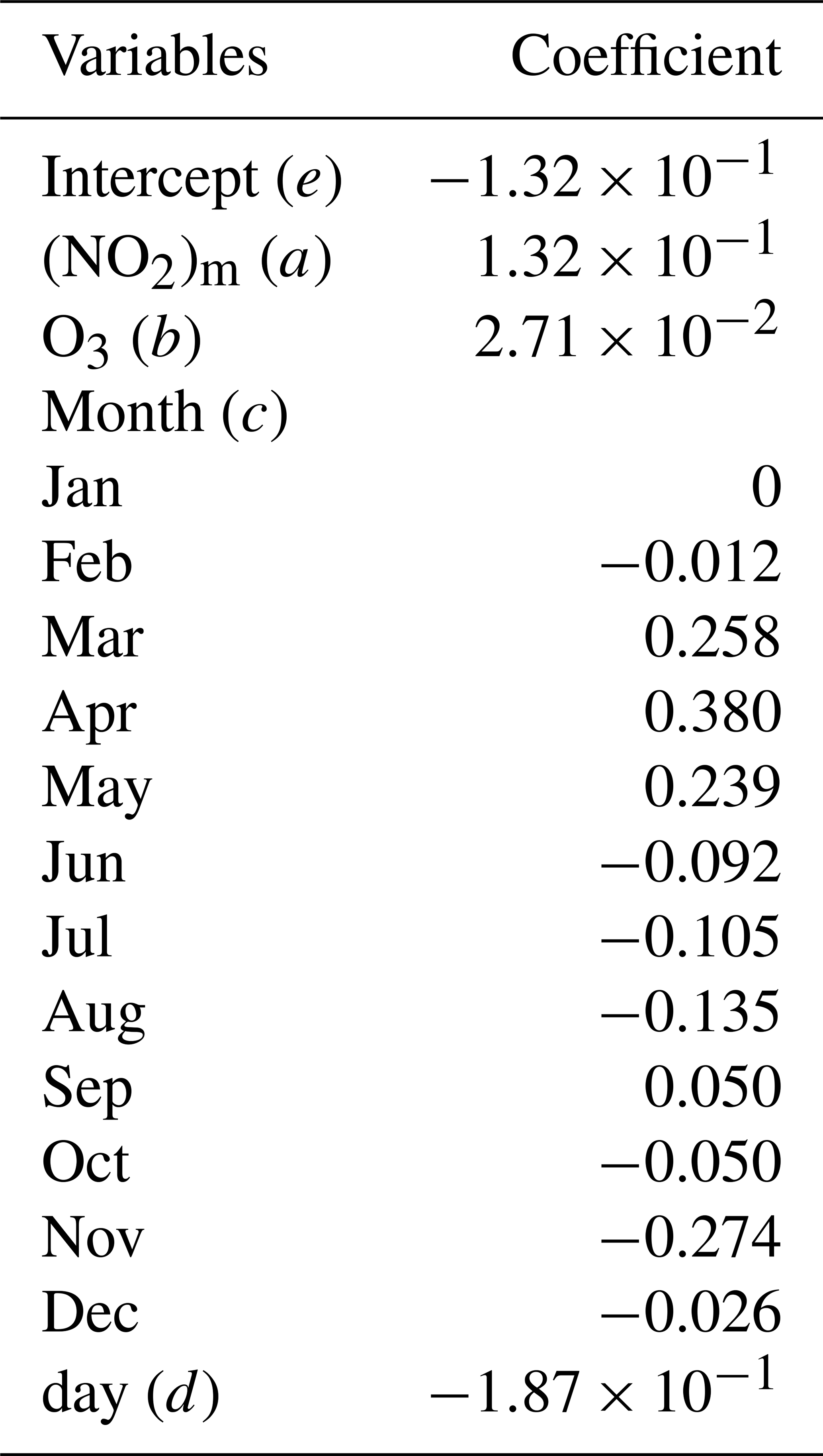
Table C2Number of wildfire-influenced and background days at each site during summer (June–September) from 2016 to 2020.

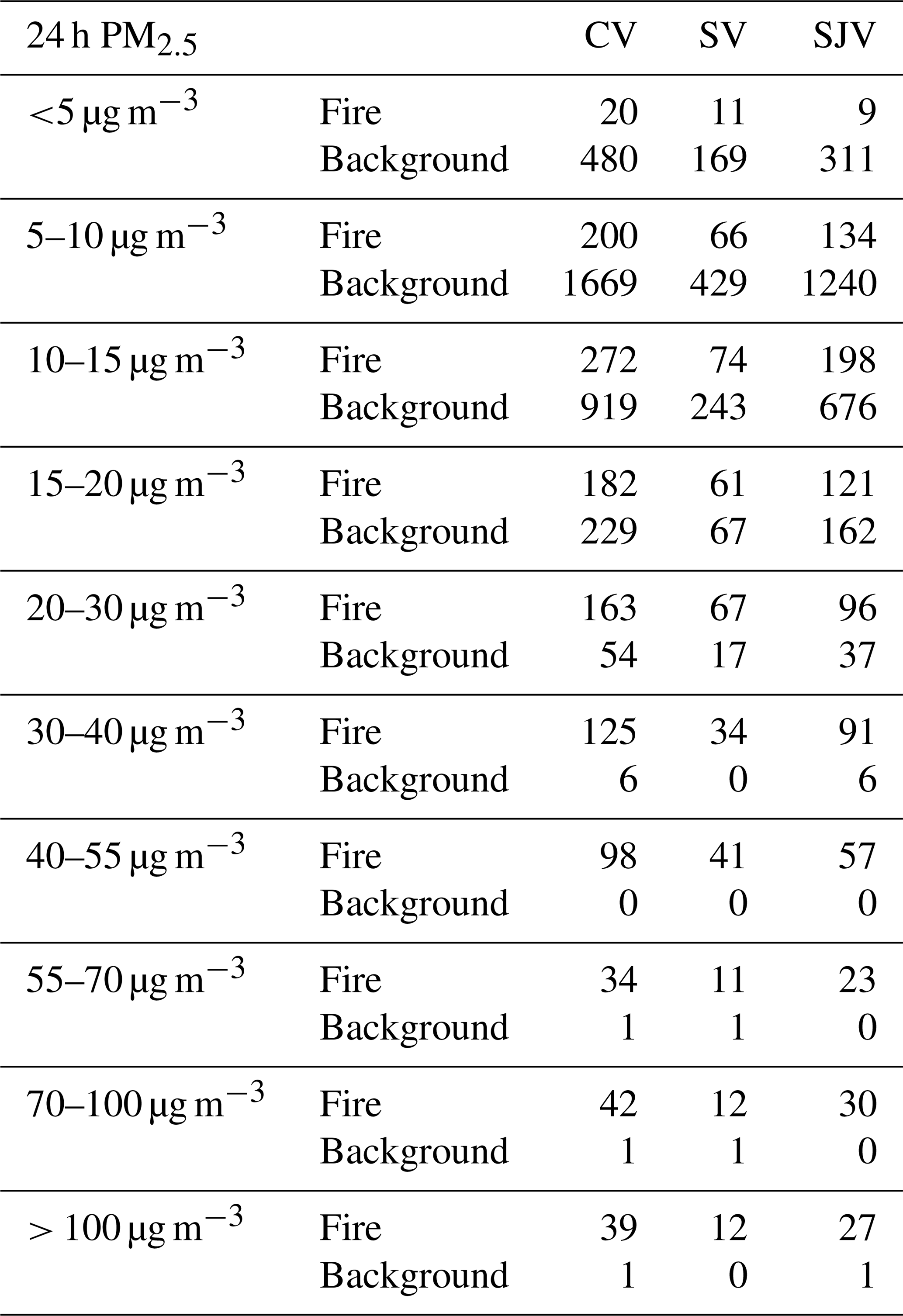
Table C4Number and percentage of the exceedances of 70 ppb MDA8 O3 at each site.
All air quality and meteorological data (Sect. 2.1) were downloaded from the Air Quality and Meteorological Information System of California Air Resources Board's (CARB) website (https://www.arb.ca.gov/aqmis2/aqmis2.php, California Air Resources Board, 2020a). The HMS products (Sect. 2.2) were provided by NOAA's Office of Satellite and Product Operations (OSPO), (https://www.ospo.noaa.gov/Products/land/hms.html, last access: 11 December 2020, NOAA, 2020b). Solar radiation measurements (Sect. 2.3) were downloaded from the CIMIS website (https://cimis.water.ca.gov/WSNReportCriteria.aspx, California Irrigation Management Information System, 2020). RASS data collected near Visalia (Sect. 2.4) were downloaded from the website of NOAA's Physical Sciences Laboratory (https://psl.noaa.gov/data/obs/datadisplay, NOAA, 2022, last access: 17 November 2020). Surface fluxes data (Sect. 2.4) of Twitchell Island and Vaira Ranch were downloaded from the AmeriFlux website (https://ameriflux.lbl.gov/, Ma et al., 2020; Knox et al., 2018, last access: 16 November 2020). NOy data (Sect. 3.2) were downloaded from the AirNow-Tech website (http://www.airnowtech.org, AirNow-Tech, 2020, last access: 17 February 2022). TOPAZ data from NOAA Earth System Research Laboratory Chemical Sciences Division during 2016 CABOTS are used in Sect. 3.3 (https://csl.noaa.gov/groups/csl3/measurements/cabots/topaz.php, last access: 3 August 2021).
KP and ICF prepared the manuscript. KP performed the majority of data analysis, including writing code, creating figures, wildfire identification based on HYSPLIT trajectories and the HMS. ICF also performed data analysis, manuscript revision, wrote responses to the reviewers and consulted with data providers.
The contact author has declared that none of the authors has any competing interests.
Publisher’s note: Copernicus Publications remains neutral with regard to jurisdictional claims in published maps and institutional affiliations.
The Tunable Optical Profiler for Aerosol and oZone (TOPAZ) lidar data were generously provided by NOAA's Earth System Research Laboratory Chemical Sciences Division from the California Baseline Ozone Transport study (CABOTS) in 2016. We thank Honza Rejmanek and colleagues at the Quality Management Branch of the Monitoring and Laboratory Division of the California Air Resources Board for tracking the quality assurance reports of the NOx instrumentation.
This research has been supported by the USDA National Institute of Food and Agriculture, [Hatch project CA-D-LAW-2481-H, “Understanding Background Atmospheric Composition, Regional Emissions, and Transport Patterns Across California”].
This paper was edited by Jerome Brioude and reviewed by two anonymous referees.
Ainsworth, E.: A. Understanding and improving global crop response to ozone pollution, Plant J., 90, 886–897, https://doi.org/10.1111/tpj.13298, 2017.
AirNow-Tech: Data Queries, MADIS [data set], https://www.airnowtech.org/data/index.cfm (last access: 3 June 2021), 2020.
Akagi, S. K., Yokelson, R. J., Burling, I. R., Meinardi, S., Simpson, I., Blake, D. R., McMeeking, G. R., Sullivan, A., Lee, T., Kreidenweis, S., Urbanski, S., Reardon, J., Griffith, D. W. T., Johnson, T. J., and Weise, D. R.: Measurements of reactive trace gases and variable O3 formation rates in some South Carolina biomass burning plumes, Atmos. Chem. Phys., 13, 1141–1165, https://doi.org/10.5194/acp-13-1141-2013, 2013.
Alvarado, M. J., Logan, J. A., Mao, J., Apel, E., Riemer, D., Blake, D., Cohen, R. C., Min, K.-E., Perring, A. E., Browne, E. C., Wooldridge, P. J., Diskin, G. S., Sachse, G. W., Fuelberg, H., Sessions, W. R., Harrigan, D. L., Huey, G., Liao, J., Case-Hanks, A., Jimenez, J. L., Cubison, M. J., Vay, S. A., Weinheimer, A. J., Knapp, D. J., Montzka, D. D., Flocke, F. M., Pollack, I. B., Wennberg, P. O., Kurten, A., Crounse, J., Clair, J. M. St., Wisthaler, A., Mikoviny, T., Yantosca, R. M., Carouge, C. C., and Le Sager, P.: Nitrogen oxides and PAN in plumes from boreal fires during ARCTAS-B and their impact on ozone: an integrated analysis of aircraft and satellite observations, Atmos. Chem. Phys., 10, 9739–9760, https://doi.org/10.5194/acp-10-9739-2010, 2010.
Baker, K. R., Woody, M. C., Valin, L., Szykman, J., Yates, E. L., Iraci, L. T., Choi, H. D., Soja, A. J., Koplitz, S. N., Zhou, L. Campuzano-Jost, P. Jimenez, J. L., and Hair, J. W.: Photochemical model evaluation of 2013 California wild fire air quality impacts using surface, aircraft, and satellite data, Sci. Total Environ., 637, 1137–1149, https://doi.org/10.1016/j.scitotenv.2018.05.048, 2018.
Baldocchi, D., Knox, S., Dronova, I., Verfaillie, J., Oikawa, P., Sturtevant, C., Matthes, J. H., and Detto, M.: The impact of expanding flooded land area on the annual evaporation of rice, Agr. Forest Meteorol., 223, 181–193, https://doi.org/10.1016/j.agrformet.2016.04.001, 2016.
Baylon, P., Jaffe, D. A., Wigder, N. L., Gao, H., and Hee, J.: Ozone enhancement in western US wildfire plumes at the Mt. Bachelor Observatory: The role of NOx, Atmos. Environ., 109, 297–304, https://doi.org/10.1016/j.atmosenv.2014.09.013, 2015.
Baylon, P., Jaffe, D. A., Hall, S. R., Ullmann, K., Alvarado, M. J., and Lefer, B. L.: Impact of biomass burning plumes on photolysis rates and ozone formation at the Mount Bachelor Observatory, J. Geophys. Res.-Atmos., 123, 2272–2284, https://doi.org/10.1002/2017JD027341, 2018.
Bianco, L., Djalalova, I. V., King, C. W., and Wilczak, J. M.: Diurnal evolution and annual variability of boundary-layer height and its correlation to other meteorological variables in California's Central Valley, Bound.-Lay. Meteorol., 140, 491–511, https://doi.org/10.1007/s10546-011-9622-4, 2011.
Brey, S. J. and Fischer, E. V.: Smoke in the city: how often and where does smoke impact summertime ozone in the United States?, Environ. Sci. Technol., 50, 1288–1294, https://doi.org/10.1021/acs.est.5b05218, 2016.
Brey, S. J., Barnes, E. A., Pierce, J. R., Wiedinmyer, C., and Fischer, E. V.: Environmental conditions, ignition type, and air quality impacts of wildfires in the southeastern and western United States, Earth's Future, 6, 1442–1456, https://doi.org/10.1029/2018EF000972, 2018a.
Brey, S. J., Ruminski, M., Atwood, S. A., and Fischer, E. V.: Connecting smoke plumes to sources using Hazard Mapping System (HMS) smoke and fire location data over North America, Atmos. Chem. Phys., 18, 1745–1761, https://doi.org/10.5194/acp-18-1745-2018, 2018b.
Brey, S. J., Barnes, E. A., Pierce, J. R., Swann, A. L., and Fischer, E. V.: Past variance and future projections of the environmental conditions driving western US summertime wildfire burn area, Earth's Future, 9, e2020EF001645, https://doi.org/10.1029/2020EF001645, 2021.
Briggs, N. L., Jaffe, D. A., Gao, H., Hee, J. R., Baylon, P. M., Zhang, Q., Zhou, S., Collier, S. C., Sampson, P. D., and Cary, R. A.: Particulate matter, ozone, and nitrogen species in aged wildfire plumes observed at the Mount Bachelor Observatory, Aerosol Air Qual. Res., 16, 3075–3087, https://doi.org/10.4209/aaqr.2016.03.0120, 2016.
Brune, W. H., Baier, B. C., Thomas, J., Ren, X., Cohen, R. C., Pusede, S. E., Browne, E. C., Goldstein, A. H., Gentner, D. R., Keutsch, F. N., Thornton, J. A., Harrold, S., Lopez-Hilfiker, F. D., and Wennberg, P. O.: Ozone production chemistry in the presence of urban plumes, Faraday Discuss., 189, 169–189, https://doi.org/10.1039/C5FD00204D, 2016.
Buysse, C. E., Kaulfus, A., Nair, U., and Jaffe, D. A.: Relationships between particulate matter, ozone, and nitrogen oxides during urban smoke events in the western US, Environ. Sci. Technol., 53, 12519–12528, https://doi.org/10.1021/acs.est.9b05241, 2019.
California Air Resources Board: Air Quality and Meteorological Information System, California Air Resources Board [data set], https://www.arb.ca.gov/aqmis2/aqmis2.php (last access: 17 February 2022), 2020.
California Irrigation Management Information System: Solar Radiation Measurements, CIMIS Stations Reports [data set], https://cimis.water.ca.gov/WSNReportCriteria.aspx (last access: 17 February 2022), 2020.
David, A. T., Asarian, J. E., and Lake, F. K.: Wildfire smoke cools summer river and stream water temperatures, Water Resour. Res., 54, 7273–7290, https://doi.org/10.1029/2018WR022964, 2018.
de Gouw, J. A. and Lovejoy, E. R.: Reactive uptake of ozone by liquid organic compounds, Geophys. Res. Lett., 25, 931–934, https://doi.org/10.1029/98GL00515, 1998.
Dunlea, E. J., Herndon, S. C., Nelson, D. D., Volkamer, R. M., San Martini, F., Sheehy, P. M., Zahniser, M. S., Shorter, J. H., Wormhoudt, J. C., Lamb, B. K., Allwine, E. J., Gaffney, J. S., Marley, N. A., Grutter, M., Marquez, C., Blanco, S., Cardenas, B., Retama, A., Ramos Villegas, C. R., Kolb, C. E., Molina, L. T., and Molina, M. J.: Evaluation of nitrogen dioxide chemiluminescence monitors in a polluted urban environment, Atmos. Chem. Phys., 7, 2691–2704, https://doi.org/10.5194/acp-7-2691-2007, 2007.
Faloona, I. C., Chiao, S., Eiserloh, A. J., Alvarez, R. J., Kirgis, G., Langford, A. O., Senff, C. J., Caputi, D., Hu, A., Iraci, L. T., Yates, E. L., Marrero, J. E., Ryoo, J., Conley, S., Tanrikulu, S., Xu, J., and Kuwayama, T.: The California Baseline Ozone Transport Study (CABOTS), Bull. Am. Meteorol. Soc., 101, E427–E445, https://doi.org/10.1175/BAMS-D-18-0302.1, 2020.
Fischer, E. V., Jaffe, D. A., Reidmiller, D. R., and Jaegle, L.: Meteorological controls on observed peroxyacetyl nitrate at Mount Bachelor during the spring of 2008, J. Geophys. Res.-Atmos., 115, D03302, https://doi.org/10.1029/2009JD012776, 2010.
Hennemuth, B. and Lammert, A.: Determination of the atmospheric boundary layer height from radiosonde and lidar backscatter, Bound.-Lay. Meteorol., 120, 181–200, https://doi.org/10.1007/s10546-005-9035-3, 2006.
Jaffe, D. A. and Wigder, N. L.: Ozone production from wildfires: A critical review, Atmos. Environ., 51, 1–10, https://doi.org/10.1016/j.atmosenv.2011.11.063, 2012.
Jenkin, M. E. and Hayman, G. D.: Photochemical ozone creation potentials for oxygenated volatile organic compounds: sensitivity to variations in kinetic and mechanistic parameters, Atmos. Environ., 33, 1275–1293, https://doi.org/10.1016/S1352-2310(98)00261-1, 1999.
Knox, S., Matthes, J. H., Verfaillie, J., and Baldocchi, D.: AmeriFlux BASE US-Twt Twitchell Island, Ver. 6-5, AmeriFlux AMP [Data set], https://doi.org/10.17190/AMF/1246140, 2018.
Langford, A. O., Alvarez, R. J., Brioude, J., Caputi, D., Conley, S. A., Evan, S., Faloona, I. C., Iraci, L. T., Kirgis, G., Marrero, J. E., Ryoo, J. M., Senff, C. J., and Yates, E. L.: Ozone production in the Soberanes smoke haze: Implications for air quality in the San Joaquin Valley during the California Baseline Ozone Transport Study, J. Geophys. Res.-Atmos., 125, e2019JD031777, https://doi.org/10.1029/2019JD031777, 2020.
Leighton, P. A.: Photochemistry of Air Pollution, Vol. 9, Academic Press, New York, USA, ISBN 9780124422506, 1961.
Leukauf, D., Gohm, A., and Rotach, M. W.: Quantifying horizontal and vertical tracer mass fluxes in an idealized valley during daytime, Atmos. Chem. Phys., 16, 13049–13066, https://doi.org/10.5194/acp-16-13049-2016, 2016.
Lin, M., Horowitz, L. W., Payton, R., Fiore, A. M., and Tonnesen, G.: US surface ozone trends and extremes from 1980 to 2014: quantifying the roles of rising Asian emissions, domestic controls, wildfires, and climate, Atmos. Chem. Phys., 17, 2943–2970, https://doi.org/10.5194/acp-17-2943-2017, 2017.
Lin, X., Trainer, M., and Liu, S. C.: On the nonlinearity of the tropospheric ozone production, J. Geophys. Res.-Atmos., 93, 15879–15888, https://doi.org/10.1029/JD093iD12p15879, 1988.
Lippmann, H. H., Jesser, B., and Schurath, U.: The rate constant of NO + O3 → NO2 + O2 in the temperature range of 283–44 K, Int. J. Chem. Kinet., 12, 547–554, https://doi.org/10.1002/kin.550120805, 1980.
Liu, C., Fedorovich, E., Huang, J., Hu, X. M., Wang, Y., and Lee, X.: Impact of aerosol shortwave radiative heating on entrainment in the atmospheric convective boundary layer: A large-eddy simulation study, J. Atmos. Sci., 76, 785–799, https://doi.org/10.1175/JAS-D-18-0107.1, 2019.
Liu, S. C., Trainer, M., Fehsenfeld, F. C., Parrish, D. D., Williams, E. J., Fahey, D. W., Hübler, G., and Murphy, P. C.: Ozone production in the rural troposphere and the implications for regional and global ozone distributions, J. Geophys. Res.-Atmos., 92, 4191–4207, https://doi.org/10.1029/JD092iD04p04191, 1987.
Ma, S., Xu, L., Verfaillie, J., and Baldocchi, D.: AmeriFlux BASE US-Var Vaira Ranch-Ione, Ver. 16-5, AmeriFlux AMP [data set], https://doi.org/10.17190/AMF/1245984, 2021.
Mannschreck, K., Gilge, S., Plass-Duelmer, C., Fricke, W., and Berresheim, H.: Assessment of the applicability of NO-NO2-O3 photostationary state to long-term measurements at the Hohenpeissenberg GAW Station, Germany, Atmos. Chem. Phys., 4, 1265–1277, https://doi.org/10.5194/acp-4-1265-2004, 2004.
McClure, C. D. and Jaffe, D. A.: Investigation of high ozone events due to wildfire smoke in an urban area, Atmos. Environ., 194, 146–157, https://doi.org/10.1016/j.atmosenv.2018.09.021, 2018.
National Report of Wildland Fires and Acres Burned by State: https://www.nifc.gov/fire-information/statistics, last access: 11 December 2020.
Ninneman, M. and Jaffe, D. A.: The impact of wildfire smoke on ozone production in an urban area: Insights from field observations and photochemical box modeling, Atmos. Environ., 267, 118764, https://doi.org/10.1016/j.atmosenv.2021.118764, 2021.
NOAA: Physical Sciences Laboratory: 915 MHz Wind Profiler, Profiler Network Data and Image Library, https://psl.noaa.gov/data/obs/datadisplay/, last access: 17 November 2020a.
NOAA: The Office of Satellite and Product Operations (OSPO): Hazard Mapping System (HMS) Fire and Smoke Analysis, GOES Biomass Burning Emissions Product (GBBEP) [data set], https://www.ospo.noaa.gov/Products/land/hms.html, last access: 11 December 2020b.
NOAA: Physical Sciences Laboratory: Climate Analysis and Plotting Tools, NOAA [data set], https://psl.noaa.gov/cgi-bin/data/getpage.pl, last access: 20 April 2022, 2022.
Olszyna, K. J., Bailey, E. M., Simonaitis, R., and Meagher, J. F.: O3 and NOy relationships at a rural site, J. Geophys. Res.-Atmos., 99, 14557–14563, https://doi.org/10.1029/94JD00739, 1994.
Pahlow, M., Kleissl, J., and Parlange, M. B.: Atmospheric boundary-layer structure observed during a haze event due to forest-fire smoke, Bound.-Lay. Meteorol., 114, 53–70, https://doi.org/10.1007/s10546-004-6350-z, 2005.
Pal, S. and Haeffelin, M.: Forcing mechanisms governing diurnal, seasonal, and interannual variability in the boundary layer depths: Five years of continuous lidar observations over a suburban site near Paris, J. Geophys. Res.-Atmos., 120, 11–936, https://doi.org/10.1002/2015JD023268, 2015.
Parrish, D. D., Trainer, M., Holloway, J. S., Yee, J. E., Warshawsky, M. S., Fehsenfeld, F. C., Forbes, G. L., and Moody, J. L.: Relationships between ozone and carbon monoxide at surface sites in the North Atlantic region, J. Geophys. Res.-Atmos., 103, 13357–13376, https://doi.org/10.1029/98JD00376, 1998.
Pfister, G. G., Wiedinmyer, C., and Emmons, L. K.: Impacts of the fall 2007 California wildfires on surface ozone: Integrating local observations with global model simulations, Geophys. Res. Lett., 35, L19814, https://doi.org/10.1029/2008GL034747, 2008.
Potter, B. E.: Atmospheric properties associated with large wildfires, Int. J. Wildland Fire, 6, 71–76, https://doi.org/10.1071/WF9960071, 1996.
Pusede, S. E., Gentner, D. R., Wooldridge, P. J., Browne, E. C., Rollins, A. W., Min, K.-E., Russell, A. R., Thomas, J., Zhang, L., Brune, W. H., Henry, S. B., DiGangi, J. P., Keutsch, F. N., Harrold, S. A., Thornton, J. A., Beaver, M. R., St. Clair, J. M., Wennberg, P. O., Sanders, J., Ren, X., VandenBoer, T. C., Markovic, M. Z., Guha, A., Weber, R., Goldstein, A. H., and Cohen, R. C.: On the temperature dependence of organic reactivity, nitrogen oxides, ozone production, and the impact of emission controls in San Joaquin Valley, California, Atmos. Chem. Phys., 14, 3373–3395, https://doi.org/10.5194/acp-14-3373-2014, 2014.
Pusede, S. E., Duffey, K. C., Shusterman, A. A., Saleh, A., Laughner, J. L., Wooldridge, P. J., Zhang, Q., Parworth, C. L., Kim, H., Capps, S. L., Valin, L. C., Cappa, C. D., Fried, A., Walega, J., Nowak, J. B., Weinheimer, A. J., Hoff, R. M., Berkoff, T. A., Beyersdorf, A. J., Olson, J., Crawford, J. H., and Cohen, R. C.: On the effectiveness of nitrogen oxide reductions as a control over ammonium nitrate aerosol, Atmos. Chem. Phys., 16, 2575–2596, https://doi.org/10.5194/acp-16-2575-2016, 2016.
Reid, J. S., Koppmann, R., Eck, T. F., and Eleuterio, D. P.: A review of biomass burning emissions part II: intensive physical properties of biomass burning particles, Atmos. Chem. Phys., 5, 799–825, https://doi.org/10.5194/acp-5-799-2005, 2005.
Rolph, G. D., Draxler, R. R., Stein, A. F., Taylor, A., Ruminski, M. G., Kondragunta, S., Zeng, J., Huang, H. C., Manikin, G., McQueen, J. T., and Davidson, P. M.: Description and verification of the NOAA smoke forecasting system: the 2007 fire season, Weather Forecast., 24, 361–378, https://doi.org/10.1175/2008WAF2222165.1, 2009.
Rombout, P. J., Lioy, P. J., and Goldstein, B. D.: Rationale for an eight-hour ozone standard, J. Air Pollut. Control Assoc., 36, 913–917, https://doi.org/10.1080/00022470.1986.10466130, 1986.
Ruminski, M., Kondragunta, S., Draxler, R., and Zeng, J.: Recent changes to the hazard mapping system, in: Proceedings of the 15th International Emission Inventory Conference, New Orleans, USA, 15–18 May 2006, Vol. 15, p. 18, 2006.
Selimovic, V., Yokelson, R. J., McMeeking, G. R., and Coefield, S.: In situ measurements of trace gases, PM, and aerosol optical properties during the 2017 NW US wildfire smoke event, Atmos. Chem. Phys., 19, 3905–3926, https://doi.org/10.5194/acp-19-3905-2019, 2019.
Selimovic, V., Yokelson, R. J., McMeeking, G. R., and Coefield, S.: Aerosol mass and optical properties, smoke influence on O3, and high NO3 production rates in a western US city impacted by wildfires, J. Geophys. Res.-Atmos., 125, e2020JD032791, https://doi.org/10.1029/2020JD032791, 2020.
Sillman, S.: The relation between ozone, NOx and hydrocarbons in urban and polluted rural environments, Atmos. Environ., 33, 1821–1845, https://doi.org/10.1016/S1352-2310(98)00345-8, 1999.
Sillman, S. and Samson, P. J.: Impact of temperature on oxidant photochemistry in urban, polluted rural and remote environments, J. Geophys. Res.-Atmos., 100, 11497–11508, https://doi.org/10.1029/94JD02146, 1995.
Simon, H., Reff, A., Wells, B., Xing, J., and Frank, N.: Ozone trends across the United States over a period of decreasing NOx and VOC emissions, Environ. Sci. Technol., 49, 186–195, https://doi.org/10.1021/es504514z, 2015.
Singh, H. B., Cai, C., Kaduwela, A., Weinheimer, A., and Wisthaler, A.: Interactions of fire emissions and urban pollution over California: Ozone formation and air quality simulations, Atmos. Environ., 56, 45–51, https://doi.org/10.1016/j.atmosenv.2012.03.046, 2012.
Standard operating procedures for ambient air monitoring: https://www.atmospheric-chemistry-and-physics.net/submission.html#manuscriptcomposition (last access: 17 February 2022), 2021.
Stavros, E. N., Abatzoglou, J. T., McKenzie, D., and Larkin, N. K.: Regional projections of the likelihood of very large wildland fires under a changing climate in the contiguous Western United States, Climatic Change, 126, 455–468, https://doi.org/10.1007/s10584-014-1229-6, 2014.
Stein, A. F., Draxler, R. R., Rolph, G. D., Stunder, B. J., Cohen, M. D., and Ngan, F.: NOAA's HYSPLIT atmospheric transport and dispersion modeling system, Bull. Am. Meteorol. Soc., 96, 2059–2077, https://doi.org/10.1175/BAMS-D-14-00110.1, 2015.
Steinbacher, M., Zellweger, C., Schwarzenbach, B., Bugmann, S., Buchmann, B., Ordóñez, C., Prévôt, A. S., and Hueglin, C.: Nitrogen oxide measurements at rural sites in Switzerland: Bias of conventional measurement techniques, J. Geophys. Res.-Atmos., 112, D11307, https://doi.org/10.1029/2006JD007971, 2007.
Steiner, A. L., Davis, A. J., Sillman, S., Owen, R. C., Michalak, A. M., and Fiore, A. M.: Observed suppression of ozone formation at extremely high temperatures due to chemical and biophysical feedbacks, P. Natl. Acad. Sci. USA, 107, 19685–19690, https://doi.org/10.1073/pnas.1008336107, 2010.
Trainer, M., Parrish, D. D., Buhr, M. P., Norton, R. B., Fehsenfeld, F. C., Anlauf, K. G., Bottenheim, J. W., Tang, Y. Z., Wiebe, H. A., Roberts, J. M., Tanner, R. L., Newman, L., Bowersox, V. C., Meagher, J. F., Olszyna, K. J., Rodgers, M. O., Wang, T., Berresheim, H., Demerjian, K. L., and Roychowdhury, U. K.: Correlation of ozone with NOy in photochemically aged air, J. Geophys. Res.-Atmos., 98, 2917–2925, https://doi.org/10.1029/92JD01910, 1993.
Trebs, I., Bohn, B., Ammann, C., Rummel, U., Blumthaler, M., Königstedt, R., Meixner, F. X., Fan, S., and Andreae, M. O.: Relationship between the NO2 photolysis frequency and the solar global irradiance, Atmos. Meas. Tech., 2, 725–739, https://doi.org/10.5194/amt-2-725-2009, 2009.
Trousdell, J. F., Conley, S. A., Post, A., and Faloona, I. C.: Observing entrainment mixing, photochemical ozone production, and regional methane emissions by aircraft using a simple mixed-layer framework, Atmos. Chem. Phys., 16, 15433–15450, https://doi.org/10.5194/acp-16-15433-2016, 2016.
Trousdell, J. F., Caputi, D., Smoot, J., Conley, S. A., and Faloona, I. C.: Photochemical production of ozone and emissions of NOx and CH4 in the San Joaquin Valley, Atmos. Chem. Phys., 19, 10697–10716, https://doi.org/10.5194/acp-19-10697-2019, 2019.
Val Martín, M. V., Honrath, R. E., Owen, R. C., Pfister, G., Fialho, P., and Barata, F.: Significant enhancements of nitrogen oxides, black carbon, and ozone in the North Atlantic lower free troposphere resulting from North American boreal wildfires, J. Geophys. Res.-Atmos., 111, D23S60, https://doi.org/10.1029/2006JD007530, 2006.
Volz-Thomas, A., Pätz, H. W., Houben, N., Konrad, S., Mihelcic, D., Klüpfel, T., and Perner, D.: Inorganic trace gases and peroxy radicals during BERLIOZ at Pabstthum: An investigation of the photostationary state of NOx and O3, J. Geophys. Res.-Atmos., 108, PHO 4-1–PHO 4-15, https://doi.org/10.1029/2001JD001255, 2003.
Wendisch, M., Mertes, S., Ruggaber, A., and Nakajima, T.: Vertical profiles of aerosol and radiation and the influence of a temperature inversion: Measurements and radiative transfer calculations, J. Appl. Meteorol., 35, 1703–1715, 1996.
Xu, Z., Wang, T., Xue, L. K., Louie, P. K., Luk, C. W., Gao, J., Wang, S. L., Chai, F. H., and Wang, W. X.: Evaluating the uncertainties of thermal catalytic conversion in measuring atmospheric nitrogen dioxide at four differently polluted sites in China, Atmos. Environ., 76, 221–226, https://doi.org/10.1016/j.atmosenv.2012.09.043, 2013.
Zhang, L., Jacob, D. J., Yue, X., Downey, N. V., Wood, D. A., and Blewitt, D.: Sources contributing to background surface ozone in the US Intermountain West, Atmos. Chem. Phys., 14, 5295–5309, https://doi.org/10.5194/acp-14-5295-2014, 2014.
Zhong, S., Whiteman, C. D., and Bian, X.: Diurnal evolution of three-dimensional wind and temperature structure in California's Central Valley, J. Appl. Meteorol., 43, 1679–1699, https://doi.org/10.1175/JAM2154.1, 2004.