Simulating the radiative forcing of oceanic dimethylsulfide (DMS) in Asia based on machine learning estimates

Dimethylsulfide (DMS) emitted from seawater is a key precursor to new particle formation and acts as a regulator in Earth's warming climate system. However, DMS's effects are not well understood in various ocean regions. In this study, we estimated DMS emissions based on a machine learning method and used the GEOS-Chem global 3D chemical transport model coupled with the TwO Moment Aerosol Sectional (TOMAS) microphysics scheme to simulate the atmospheric chemistry and radiative effects of DMS. The contributions of DMS to atmospheric ${{\mathrm{SO}}_{\mathrm{4}}}^{\mathrm{2}-}$ aerosol and cloud condensation nuclei (CCN) concentrations along with the radiative effects over the Asian region were evaluated for the first time. First, we constructed novel monthly resolved DMS emissions ($\mathrm{0.5}{}^{\circ }\times \mathrm{0.5}{}^{\circ }$) for the year 2017 using a machine learning model; 4351 seawater DMS measurements (including the recent measurements made over the Chinese seas) and 12 relevant environment parameters were selected for model training. We found that the model could predict the observed DMS concentrations with a correlation coefficient of 0.75 and fill the values in regions lacking observations. Across the Asian seas, the highest seasonal mean DMS concentration occurred in March–April–May (MAM), and we estimate the annual DMS emission flux of 1.25 Tg (S), which is equivalent to 15.4 % of anthropogenic sulfur emissions over the entire simulation domain (which covered most of Asia) in 2017. The model estimates of DMS and methane sulfonic acid (MSA), using updated DMS emissions, were evaluated by comparing them with cruise survey experiments and long-term online measurement site data. The improvement in model performance can be observed compared with simulation results derived from the global-database DMS emissions. The relative contributions of DMS to ${{\mathrm{SO}}_{\mathrm{4}}}^{\mathrm{2}-}$ and CCN were higher in remote oceanic areas, contributing 88 % and 42 % of all sources, respectively. Correspondingly, the sulfate direct radiative forcing (DRF) and indirect radiative forcing (IRF) contributed by DMS ranged from −200 to −20 mW m⁻² and from −900 to −100 mW m⁻², respectively, with levels varying by season. The strong negative IRF is mainly over remote ocean regions (−900 to −600 mW m⁻²). Generally, the magnitude of IRF derived by DMS was twice as large as its DRF. This work provides insights into the source strength of DMS and the impact of DMS on climate and addresses knowledge gaps related to factors controlling aerosols in the marine boundary layer and their climate impacts.

1 Introduction

Ocean-emitted dimethylsulfide (DMS) is a precursor of non-sea-salt ${{\mathrm{SO}}_{\mathrm{4}}}^{\mathrm{2}-}$ and controls the composition, size distribution, and number concentration of aerosols over the remote oceanic areas. ${{\mathrm{SO}}_{\mathrm{4}}}^{\mathrm{2}-}$ directly influences the climate system directly by reflecting solar radiation back into the space and indirectly by acting as cloud condensation nuclei (CCN) and altering the albedo of clouds and changing cloud radiative properties (Andreae and Rosenfeld, 2008). The “CLAW” hypothesis proposed by Charlson et al. (1987) assumed that negative feedback interactions between ocean plankton and the climate system, where the Earth system acted to buffer itself from warming, were linked through DMS production. Thereafter, several studies found significant impacts of DMS-induced aerosols on CCN and cloud albedos in remote oceans (Park et al., 2017; Quinn et al., 2017; Kulmala et al., 2014; Vallina and Simó, 2007), which lent credence to the CLAW hypothesis. Nevertheless, due to the low sensitivity of each step of the interactions to changes in force factors in the CLAW climate feedback loop (e.g., low sensitivity of DMS production to changes in incident solar radiation), Quinn and Bates (2011) disproved the hypothesis. Whether the CLAW climate feedback is positive or negative is still uncertain, and further research is needed to quantify the climate effects of DMS.

Building an accurate emission inventory is key to simulating the climate effects of DMS. As many previous studies have shown (Chen et al., 2018; Hodshire et al., 2019; Rap et al., 2013; Yang et al., 2017; Zhao et al., 2021), the marine DMS emissions used in numerical models are mainly estimated using an interpolation scheme (Kettle et al., 1999; Lana et al., 2011), which estimates DMS climatology by interpolating observed DMS data at limited sites to the global ocean. Previously, observations from the Global Surface Seawater DMS Database have been grouped into 57 ecological geographic ocean provinces, and weighted interpolations from nearby provinces have been used to fill the values without observations. Wang et al. (2020) pointed out that there are uncertainties in using spatial and temporal averaged data to fill regions without observations. However, artificial neural networks can potentially be trained and used to fill measurement gaps (Wang et al., 2020). Galí et al. (2018) created a remote sensing algorithm to estimate DMS concentrations which is based on the relationship between a precursor of DMS and plankton light exposure. Their results (Galí et al., 2018) indicated that the remote sensing algorithms have better ability to reproduce the climatological features of DMS seasonality than interpolated DMS climatologies, which also outweigh the disadvantage of the interpolation scheme used in a previous study (Lana et al., 2011). In a recent study (Bell et al., 2021), long-term in situ DMS measurements conducted in the North Atlantic Ocean from 2015 to 2018 were compared with the interpolated DMS climatologies (Lana et al., 2011), predicted DMS concentrations from the remote sensing algorithm (Galí et al., 2018), and a neural network approach (Wang et al., 2020). The analysis revealed that both the remote sensing algorithm and the neural network model were better able to reproduce the seawater DMS trends better than the interpolated climatologies. However, DMS predictions from two of the models (Galí et al., 2018; Wang et al., 2020) underpredicted DMS concentrations, likely because the primary biological processes of DMS production were not accounted for (Bell et al., 2021).

There are several modeling studies which have quantified the aerosol direct and indirect radiative forcings of DMS on a global scale. The global annual mean DMS aerosol indirect radiative forcing estimates have ranged from −6.55 to −0.23 W m⁻² in previous studies (Mahajan et al., 2015; Thomas et al., 2010; Rap et al., 2013; Yang et al., 2017; Jin et al., 2018). However, there have been few studies that have reported the radiative effect of DMS on a regional scale. Choi et al. (2020) adopted an empirical algorithm to estimate DMS concentrations and calculated the direct radiative effect of DMS aerosol to be −1.3 W m⁻² for the year 2014–2016 over the East Asian seas, which was higher than the global average results (Yang et al., 2017; Rap et al., 2013). There were no evaluations of the DMS predictions in the seawater or atmosphere in these studies, leading to an unknown reliability of the results. The annual-mean direct radiative forcings due to DMS-produced aerosol were −0.2 to −0.1 W m⁻² over East Asia reported by Li et al. (2019), who used a DMS climatology (Lana et al., 2011) with $\mathrm{1}{}^{\circ }\times \mathrm{1}{}^{\circ }$ horizontal resolution for radiative forcing calculation. As mentioned before, some uncertainties in the DMS climatology estimated by an interpolation scheme and coarse grid ($\mathrm{1}{}^{\circ }\times \mathrm{1}{}^{\circ }$) may not be appropriate for regional simulations. In the previous studies, Li et al. (2020a, b) used long-term DMS measurements in 2011, 2013, 2015, 2016, and 2017 from a series of shipboard field experiments and performed interpolation to map DMS concentrations in the Chinese seas. The newest DMS measurements were used to explore the impact of DMS on air quality over coastal areas of China, but the radiative effect of DMS was not reported.

To our knowledge, this is the first systematic study of the Asian region that quantifies the impacts of DMS on sulfate, particle number concentration, and radiative forcing by using a state-of-the-art aerosol microphysics model coupled to a global 3D chemical transport model. In this study, we developed the regional DMS emissions for the year 2017 by training eXtreme Gradient Boosting (XGBoost) machine learning algorithms (Chen and Guestrin, 2016) using a newly updated dataset. Then, the model estimates of DMS and methane sulfonic acid (MSA) were evaluated by comparing the model simulations with shipboard field measurements and long-term online measurement site data. Finally, the annual-average and seasonal impacts of DMS on sulfate/CCN concentrations and direct/indirect radiative forcing were quantified.

2 Methods and data

2.1 GEOS-Chem-TOMAS

In this study, GEOS-Chem version 12.9.3 (https://doi.org/10.5281/zenodo.3974569, last access: 25 March 2021) coupled with the online TOMAS aerosol microphysics model (Adams and Seinfeld, 2002) was adopted to calculate atmospheric aerosol size, number, and mass concentrations from marine DMS emissions. TOMAS was used to simulate aerosol microphysics processes (i.e., nucleation, coagulation, condensation, cloud processing). The advantage of TOMAS is the full aerosol size resolution for all chemical species and the conservation of aerosol number, which allows modelers to construct aerosol and CCN number budgets that balance. GEOS-Chem-TOMAS (GC-TOMAS) has been used in a range of previous studies (Kodros and Pierce, 2017; Pierce and Adams, 2006; Kodros et al., 2016; D'Andrea et al., 2013; Westervelt et al., 2013; Lee et al., 2009; Trivitayanurak et al., 2008; Pierce et al., 2007; Adams and Seinfeld, 2002; Jathar et al., 2020). The model contains detailed hydrocarbon–nitrogen oxide (NO_x)–ozone(O₃)–volatile organic compound (VOC)–bromine oxide (BrO_x) tropospheric chemistry (Bey et al., 2001) and aerosol species (including sulfate, nitrate, ammonium, black carbon, organic carbon, mineral dust, and sea salt) (Duncan Fairlie et al., 2007; Pye et al., 2009; Alexander et al., 2005; Park et al., 2004) that are fully coupled to gas-phase chemistry, with the ISORROPIA II algorithm to calculate the thermodynamic equilibrium between aerosols and their gas-phase precursors (Fountoukis and Nenes, 2007). The model includes a detailed wet and dry deposition scheme for aerosols and gas species which have been described in previous studies (Wesely, 2007; Liu et al., 2001; Wang et al., 1998; Amos et al., 2012). This version of GC-TOMAS tracks the total aerosol particle number and the mass of each aerosol species (sulfate, mineral dust, sea salt, hydrophilic and hydrophobic organic carbon, externally and internally mixed elemental carbon, and aerosol water) across 15 logarithmically size bins ranging from 3 nm to 10 µm (Lee and Adams, 2012; Lee et al., 2013). Since the ammonium nitrate size distribution is not explicitly tracked with GC-TOMAS, we assume that it follows the aerosol water distribution (Bilsback et al., 2020a, b).

The simulation domain covering most of Asia (11^∘ S to 55^∘ N, 60–150^∘ E) was discretized with a horizontal grid resolution of $\mathrm{0.5}{}^{\circ }\times \mathrm{0.625}{}^{\circ }$ and 47 vertical layers and uses the Modern-Era Retrospective Analysis for Research and Applications version (MERRA-2)-assimilated meteorological field for meteorological inputs (Gelaro et al., 2017). To assess radiative impacts of DMS emissions at a regional scale, we performed three different annual simulations for the year 2017 (Table 1). The “XG” simulation represents DMS emissions that were calculated from our updated DMS emissions estimates (see Sect. 2.3), and the “LANA” simulation refers to DMS emissions from Lana DMS climatology (Lana et al., 2011), which is the default setting in the current version of the Geos-Chem model. The “ND” simulation has DMS emissions turned off. Each simulation was conducted with a 1-month spin-up period (December 2016). The boundary conditions for the simulation domain were obtained from global simulations at $\mathrm{2}{}^{\circ }\times \mathrm{2.5}{}^{\circ }$ with 47 vertical layers.

Table 1 Description of the simulation.

For anthropogenic emissions in Asia, we used the recently updated global anthropogenic emission inventories ($\mathrm{0.5}{}^{\circ }\times \mathrm{0.5}{}^{\circ }$) or the year 2017 from the open-source Community Emissions Data System (CEDS) (McDuffie et al., 2020), which applied scale factors from Zheng et al. (2018) to update China's emissions for the year 2017. Since there is a significant reduction (62 %) in SO₂ emissions in China from 2010 to 2017 (Zheng et al., 2018), updated emissions for China are crucial for quantifying contributions of biogenic sulfur sources over Asia. Biomass burning emissions in GC-TOMAS are obtained from the Global Fire Emissions Database Version 4 (van der Werf et al., 2017). Dust, biogenic VOCs, sea salt, soil NO_x, and lighting NO_x emissions are calculated online based on the MERRA-2 meteorological field. The Dust Entrainment and Deposition (DEAD) scheme from Zender et al. (2003) was implemented in GEOS-Chem to simulate dust mobilization. The Model of Emissions of Gases and Aerosols from Nature from Guenther et al. (2012) was used to generate biogenic VOC emissions. Soil and lighting NO_x emissions are calculated by the parameterization scheme described in Hudman et al. (2012) and Price and Rind (1992), respectively.

The sea–air flux of DMS is estimated using the following the empirical formula as described in Lana et al. (2011):

$$\begin{array}{}\text{(1)}& F=C_{\mathrm{w}}\times k_{\mathrm{w}}\times (\mathrm{1}-\mathit{\gamma }),\end{array}$$

where C_w is the seawater DMS concentrations, k_w is the water side gas transfer velocity and γ is the atmospheric gradient fraction. In this study, we selected the Nightingale et al. (2000) parameterization (hereafter N00) for k_w to represent the DMS emissions over the global ocean.

2.2 Radiative forcing calculation scheme

To calculate the top-of-the-atmosphere (TOA) all-sky direct radiative forcing (DRF) and cloud-albedo indirect radiative forcing (IRF), we used the Rapid Radiative Transfer Model for Global Climate Models (RRTMG) (Iacono et al., 2008) with monthly averaged aerosol number and mass concentrations from GC-TOMAS output and meteorological variables from MERRA2. For the DRF, we calculated aerosol optical depth (AOD) single scattering albedo and the asymmetry parameter based on Mie theory (Bohren and Huffman, 1983) and refractive indices from the Global Aerosol Database (Koepke et al., 1997). In all cases, the DRE was calculated for the core-shell optical assumption, where, for each aerosol size bin, black carbon was represented as a spherical core within a homogenous shell of all other hydrophilic species. For the cloud-albedo IRF, we calculate cloud droplet number concentration (CDNC) using the activation parameterization from Abdul-Razzak and Ghan (2002). Cloud-liquid water content is prescribed from MERRA-2 and held fixed, and hence we only calculated the cloud-albedo (Twomey) indirect effect. The changes in effective cloud drop radii were estimated following the cloud-droplet-radius perturbation method used in previous studies (Rap et al., 2013; Kodros et al., 2016; Scott et al., 2014). Then, RRTMG was used to calculate the changes in TOA radiative flux from the changes affecting cloud drop radii. We limited this calculation to liquid clouds, which is a limitation in this method. More detailed information about the implementation of RRTMG in GC-TOMAS can be found in Kodros et al. (2016).

2.3 Machine learning estimates of sea-surface DMS concentration for calculating DMS emission flux

XGBoost (machine learning algorithm under the Gradient Boosting framework) was used due to its many advantages. For example, XGBoost is computationally efficient, has prediction accuracy, requires less tuning, is scalable, has been widely used in the field of geoscience (Sun et al., 2021; Ivatt and Evans, 2020; Pan, 2018; Qian et al., 2020; Silva et al., 2022; Cao et al., 2021), and generally outperformed other models. Moreover, XGBoost is good for tabular data and does not require large training datasets (Shwartz-Ziv and Armon, 2022). Thus, to better capture the nonlinear relationship between DMS and the parameters that influence it, we trained an XGBoost model with the entire dataset to predict sea surface DMS concentrations in the place of missing observations.

Figure S1 in the Supplement shows the spatial distribution of DMS measurements. The red points (1022 valid measurements) represent the local DMS observation dataset (2011, 2013, 2015, 2016, and 2017) across several Chinese seas from China Ocean University. Details can be found in our previous studies (G.-P. Yang et al., 2014, 2015; J. Yang et al., 2015; Xu et al., 2021; Zhai et al., 2020; Wu et al., 2020; Jian et al., 2019; Yu et al., 2019; Mao et al., 2021). The blue points (3329 valid measurements) represent the observations from the Global Surface Seawater DMS Database (http://saga.pmel.noaa.gov/dms/, last access: 1 May 2021). In total, 12 environmental parameters (Table S1 in the Supplement) which strongly affect the growth of phytoplankton and the production of DMS (Wang et al., 2015) were included as predictors in machine learning estimates. Satellite remotely sensed chlorophyll (Chl), photosynthetically available radiation (PAR), particulate inorganic/organic carbon (PIC/POC), and diffuse attenuation coefficient at 490 m (kd490) were from MODIS-Aqua products (daily, 8 d, and monthly Level 3-binned 4 km resolution data). Nutrient data (silicate, phosphate, and nitrate), sea surface temperature (SST), salinity, and dissolved oxygen (DO) were obtained from World Ocean Atlas 2018 (monthly 0.25^∘ and 1^∘ climatology data). Monthly mixed-layer depth (MLD) climatology ($\mathrm{0.5}{}^{\circ }\times \mathrm{0.5}{}^{\circ }$) was obtained from the Monthly Isopycnal & Mixed-layer Ocean Climatology (MIMOC). Before the implementation of the algorithm in Asia's oceans, we performed a model validation. First, the environmental parameters were matched with DMS measurements according to sampling geographical coordinates and date. Take remotely sensed Chl data, for example: if the daily binned data failed to match the DMS observed data, we used the 8 d binned data to take the place of daily binned data. After the data matching, we then conducted filtering and quality control which followed methods from Wang et al. (2020); the number of data points in the simulation domain were reduced from 4351 to 3748 observation-based datasets for in situ DMS and matched with environmental parameters. Table S1 has a description of the environmental parameters, sources, and their filtering thresholds. Avoiding the possible large latitudinal and seasonal variation in DMS, the sampling times and geographic coordinates were also included in machine learning estimates. To solve issues in data discontinuity, these datasets were converted to periodic functions as suggested in previous studies (Gade, 2010; Gregor et al., 2017; Wang et al., 2020). To verify the prediction performance of the XGBoost model, we divided the datasets into two parts: a validation dataset and a training dataset. Considering that most of the northern part of the simulation domain was land area, we selected the data from 2^∘ latitude bands between 11^∘ S and 30^∘ N as validation datasets (809 points), while the rest of the data were all used as training data (2939 points). As suggested by Wang et al. (2020), the measurement data collected from the same cruise are highly intercorrelated, and using near-neighbor values to predict validation data may cause the model overfit. So, we selected the validation data manually rather than automatically.

Figure 1 displays the validation results for the XGBoost model, which reproduced DMS concentrations with high correlation coefficients (R) of 0.75 and a low root-mean-square error (RMSE) of 1.97 µmol m⁻³. The validation statistics are comparable to other studies (R=0.73–0.81 and RMSE=1.92–2.00 µmol m⁻³) that used nonlinear/multilinear models to predict sea-surface DMS concentrations over the global ocean (Galí et al., 2018; Wang et al., 2020). Model performance for predicting DMS concentration in each season was illustrated in Table S2. Predicted DMS concentrations were slightly underestimated in comparison with validation datasets, with a mean bias (MB) of −0.59 to −0.21 µmol m⁻³ and a normalized mean bias (NMB) of −19.36 % to −6.51 % across the four seasons. A lower RMSE of 1.81 µmol m⁻³ was observed in spring. The MB and NMB in spring were smaller than those in other seasons, which indicated that the model performed best in spring. Most of the available validation datasets were concentrated in spring (about 67.9 %). Thus, the imbalanced data may lead to less ideal performance in other seasons.

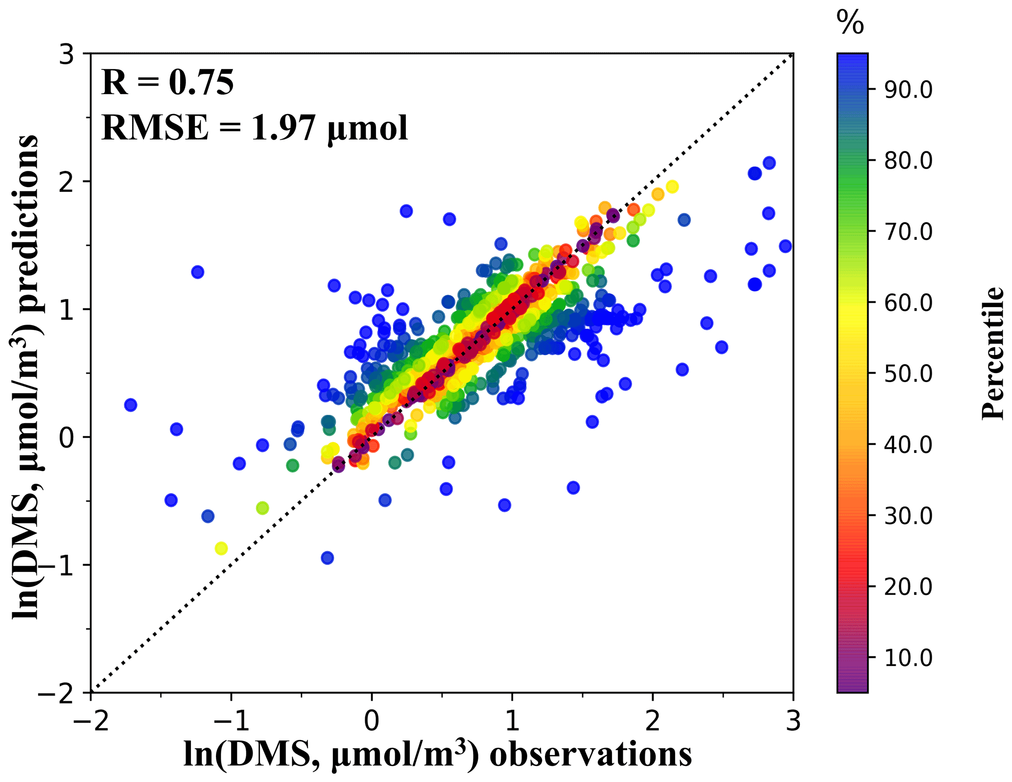
Figure 1 The scatter plot compares model predictions and observations of DMS. The color represents the percentile of distribution of absolute difference between predicted and observation data.

The advantage of utilizing a machine learning method is the ability to capture nonlinear relationships between DMS and its affecting parameters to estimate DMS concentrations with a plausible underlying basis in spatial–temporal variability. A shortcoming of the traditional geographical interpolation method is that relatively sparse data are typically interpolated to the entire ocean, which has been highlighted by previous studies (Galí et al., 2015, 2018; Wang et al., 2020). In this study, the advantage of the machine learning method is also demonstrated by comparing two different model simulations (see Sect. 3.2). In the implementation phase of the machining learning algorithm to the regional ocean, the remotely sensed datasets used to predict DMS concentrations are all from MODIS-Aqua products in 2017, and monthly climatologies were interpolated to the 8 d or monthly periods for the remotely sensed data; then, we trained the XGBoost model to obtain grid values that did not have DMS measurements. Finally, estimated DMS concentrations were temporally averaged to a seasonal period and spatially binned to the $\mathrm{0.5}{}^{\circ }\times \mathrm{0.5}{}^{\circ }$ grid for the Asian region (see Sect. 3.1).

Decision-tree-based machine learning models have a high interpretability. The SHapley Additive exPlanation regression (SHAP) (Lundberg et al., 2020) can provide a deeper understanding of model predictions, which allows for individualized feature attribution for every decision. Stirnberg et al. (2021) quantified the impact of various meteorological derivers on PM₁ concentrations by using SHAP analysis, and Silva et al. (2022) used SHAP to explore the errors in the prediction of lightning occurrence in a widely used Earth system model. In this study, SHAP was applied to investigate the importance of each predictor in model-predicted DMS concentrations.

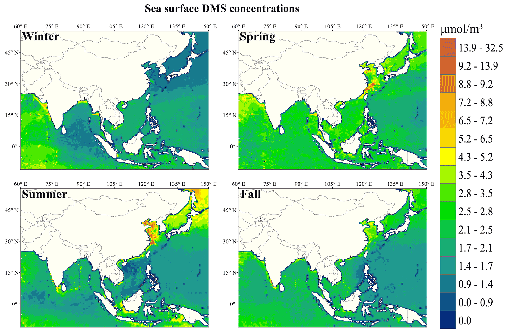
Figure 2 Sea-surface DMS concentrations predicted by the XGBoost model by season.

3 Results

3.1 Spatial and temporal patterns of the seawater DMS

Regional DMS maps for sea surface DMS concentrations predicted by XGBoost in four seasons are displayed in Fig. 2. The data show distinct seasonal variations. The highest regional mean DMS concentrations were observed in the MAM, that is, 2.52 µmol m⁻³, which was approximately 1.15, 1.24, and 1.31 times higher than those in June–July–August (JJA), September–October–November (SON), and December–January–February (DJF) (Table S3), respectively. However, according to the previous studies (Lana et al., 2011; Galí et al., 2018; Wang et al., 2020), the highest DMS concentrations usually occurred in JJA, mainly due to adequate solar irradiation and warm temperature being favorable for primary production. We assumed that this difference was caused by the fact that we examined a different statistical region compared with previous results that were based on global-scale estimates. For comparative purposes, we extracted corresponding simulation domain (Fig. 2) estimate values from global-scale estimates' results; they are listed in Table S3. Across the Asian seas, all the highest seasonal mean DMS concentrations occurred in MAM, demonstrating that our estimates agreed well with the estimates of 2.21–2.33 µmol m⁻³ reported in previous studies (Wang et al., 2020; Lana et al., 2011). As shown in Fig. S2, zonal mean DMS concentrations between 10^∘ S and 30^∘ N latitude areas of the simulation domain were higher in MAM than in JJA, but those between the 30^∘ N and 50^∘ N latitude bands were higher in JJA than in MAM. As mentioned in Sect. 2.3, most of the ocean area is concentrated in the 10^∘ S and 30^∘ N latitude band of the entire simulation domain (11^∘ S to 55^∘ N, 60–150^∘ E), which leads to the highest regional mean DMS concentrations being observed in MAM. This is most likely due to the seasonal variation of solar irradiation, because most of the ocean area (11^∘ S to 30^∘ N) in the simulation domain was influenced more by the solar irradiation in the MAM than in JJA. A similar result can be found in monthly Hovmöller diagrams of DMS climatologies, depicted by Galí et al. (2018). Throughout the four seasons, there were some high concentrations of DMS (higher than 4.3 µmol m⁻³) that appeared in different coastal areas, which is probably relevant to high nutrient and chlorophyll concentrations over the coastal areas. Galí et al. (2015) also found that most of the coastal regions have higher dimethylsulfoniopropionate (DMSP) concentrations compared with the global ocean, and DMS in the seawater was generated from the breakdown of DMSP.

Figure S3 summarizes the ranked mean SHAP values of each predictor across all prediction cases. The line ranges represent the interquartile range across the distribution. Larger SHAP value magnitudes are interpreted as more important for the prediction task as they have a larger contribution from that variable to that prediction. In our study, the most important environmental parameter for predicting DMS concentrations was Chl, followed by MLD, PAR, POC, and salinity. Above all, the SHAP value of Chl is more than double its value of MLD and PAR and much larger than all others. This is consistent with the known importance of Chl in developing predicting models of surface water DMS concentrations because of its biogenic origin (Simó and Dachs, 2002; Galí et al., 2015; Wang et al., 2020; Deng et al., 2021).

We calculated regional sea–air DMS fluxes using the N00 gas transfer velocity and DMS concentrations predicted by XGBoost (Fig. 3a). We estimated annual DMS emission fluxes of 1.25 Tg (S), corresponding to 15.4 % of the anthropogenic sulfur emissions over the entire simulation domain (covering most of Asia) in 2017. The higher estimated values of DMS fluxes (higher than 250 t (S) per grid) occurred over some coastal waters, which generally agreed well with the estimated sea surface DMS concentration distribution. The highest emission fluxes occurred over the Chinese seas (reaching up to 450 t (S) per grid). These high fluxes can be attributed to the local DMS observations dataset in the Chinese seas (red point in Fig. S1) that were included in the machine learning estimates. Our previous studies (Li et al., 2020a, b) reported that DMS emissions fluxes calculated with the local dataset are 3 times higher than the default global database (Lana et al., 2011) over most areas of the Chinese seas. The highest positive changes in DMS emissions fluxes were mainly in the areas of the East China Sea (up to 200 t (S) per grid) and some coastal regions (Fig. 3b). However, there were more negative changes in DMS emissions fluxes than positive changes in the seawater, which suggested that the sea–air DMS flux estimated in this study was generally lower than those from Lana et al. (2011). Similar results can be found in Wang et al. (2020).

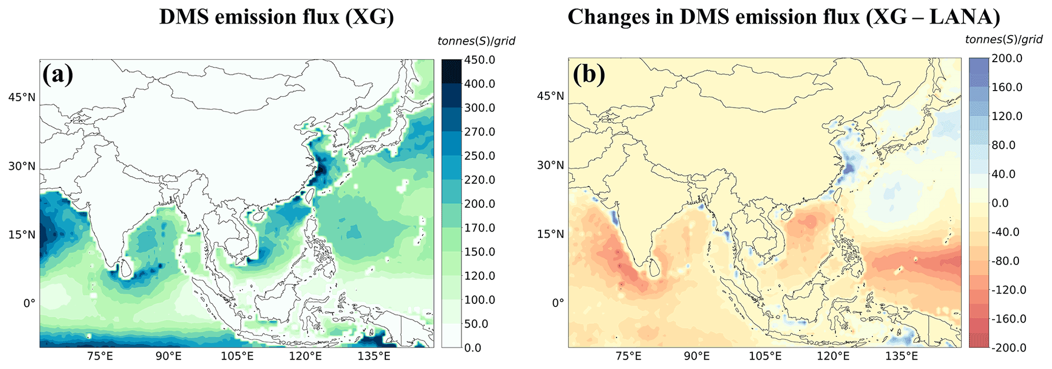
Figure 3 Panel (a) presents annual DMS emission flux calculated based on N00 flux parameterization (Nightingale et al., 2000) from XG sea surface concentrations. Panel (b) presents changes between DMS emission flux from updated (XG) and default climatology (LANA).

3.2 Model evaluation

3.2.1 Model performance of DMS and its oxidation product MSA

Modeled atmospheric DMS concentrations were compared with observations from the 2017 Cruise Survey Experiment (CSE) 1–3 (Fig. 4). Due to the discontinuities in time and gaps in observations, we averaged the whole period of each CSE observation for our comparisons. The results in Table S4 demonstrate moderate improvements in the model performance of DMS predictions when using updated DMS emissions relative to default DMS emissions; i.e., the difference between the observations and predictions (observation − prediction) became smaller (from −16.34 to 6.68 pptv for CSE 1, −21.11 to −16.17 pptv for CSE 2, and −121.57 to 117.39 pptv for CSE 3, respectively). CSE 3 had much higher DMS concentrations, because most of the measurements were from the mouth of the Changjiang River, and it is difficult for a coarse model grid ($\mathrm{0.5}{}^{\circ }\times \mathrm{0.625}{}^{\circ }$) to represent the high values that occur off coastal areas. MSA is a tracer of DMS, because it is formed exclusively from DMS (Gondwe et al., 2003). We also evaluated the model performances for MSA by comparing the model simulations with long-term online measurement site data (Zhou et al., 2021) from Hua Niao Island (Fig. 4). Figure 5 displays time series of daily mean MSA values of predictions (XG and LANA) and observations. The simulated MSA concentrations from XG and LANA are both within the range of observed values, and the trends of the MSA concentrations were relatively well reproduced, with mean values of 0.014, 0.020, and 0.023 µg m⁻³ for LANA, XG, and observations. Although in some periods LANA simulation results were closer to the observations, and XG simulations underpredicted, e.g., RMSE of 0.013 and 0.006 µg m⁻³ for LANA, 0.021 and 0.010 µg m⁻³ for XG during the periods of 21 to 25 June and 28 June to 3 July, respectively. However, on the whole, the simulation results of XG in other periods were closer to the observations than those of LANA simulation results, with RMSEs of 0.024 and 0.018 µg m⁻³ for LANA and XG, respectively.

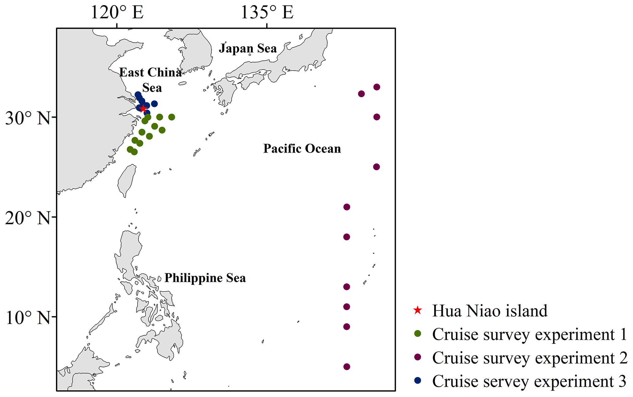
Figure 4 Locations of atmospheric DMS observations from cruise survey experiments 1–3, and the MSA observation site on Hua Niao Island.

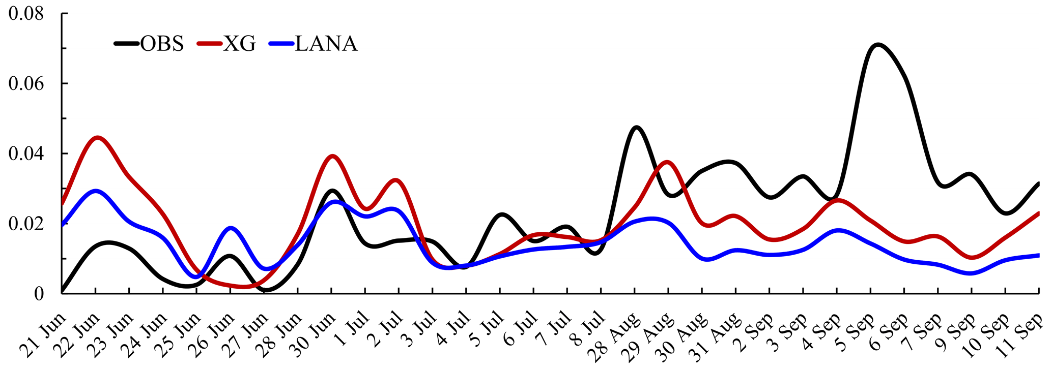
Figure 5 A comparison of simulated daily concentrations of MSA with observations at the Hua Niao Island site (units: µg m⁻³).

3.2.2 Model performance evaluation for PM_2.5, AOD, and CCN

The magnitude and distributions of PM_2.5, AOD, and CCN directly influence DRF and IRF estimates. To evaluate whether GC-TOMAS can reproduce the spatial distribution and temporal trends of these parameters over the simulation area, we evaluated model performance by comparing simulation results for XG with ground observations and satellite-retrieved estimates. Since DMS impacts PM_2.5 and CCN over the ocean and some coastal areas (see Sect. 3.3) and the ground observational data are all over land areas, we only used one of the simulations for model evaluation.

Boylan and Russell (2006) suggested that model predictions can be regarded as sufficiently accurate when the model has a mean fractional bias (MFB) $\le \pm \mathrm{30}$ % and a mean fractional error (MFE) $\le \pm \mathrm{50}$ %. Figure S4 presents the distributions of simulated annual mean PM_2.5 concentrations and observations at 366 city sites from the China National Environmental Monitoring Center (CNEMC). The model performed well against PM_2.5 observations for the year 2017, with MFB of 5.5 % and MFE of 23.1 %, which are both within the range suggested by Boylan and Russell (2006) and had a Pearson correlation coefficient (R) of 0.62. Simulated PM_2.5 concentrations were slightly underpredicted with a MB of −1.3 µg m⁻³, which is probably ascribed to underprediction of PM_2.5 in some parts of northern China. Further, uncertainties in land-based emissions inventories tend to cause different model performances in different regions.

Table S5 summarizes the collected in situ measurements of CCN concentrations in other previous studies and corresponding annual-mean simulated CCN concentrations which were used for evaluation. The MFB and MFE were 28.17 % and 34.16 %, which met the suggested benchmark; however, the model estimates underpredicted the measurements in most areas. Liu et al. (2020) adopted a satellite-based method to retrieve CCN concentrations from 2013 to 2019 and reported that they could reasonably reproduce the spatial pattern of CCN in East Asia. In this study, monthly mean GC-TOMAS CCN concentrations were compared with satellite-retrieved CCN concentrations at supersaturation levels of approximately 0.2 % from Liu et al. (2020). A total of 8 months of satellite-retrieved CCN concentrations were averaged on the MERRA-2 grid (corresponding to 667 simulation grids) for comparison (Fig. S5). The simulated CCN concentrations presented generally similar monthly variations when compared with the satellite-retrieved concentrations. The modeled concentrations had a MFB of 17.23 % and a MFE of 37.28 %, both meeting the criteria suggested by Boylan and Russell (2006). The GC-TOMAS CCN concentrations (430 cm⁻³) for 8 months underestimated the satellite-retrieved concentrations (587 cm⁻³). This underestimation is more apparent in July, August, September, and November. However, for other months (February, April, May, and June), the simulated CCN concentrations only slightly underpredicted observations with a MB of −75 cm⁻³. This difference is more likely attributable to differences in model performance in different regions. For example, the underpredictions of CCN in May were mainly distributed in the eastern coastal area of China, the Korean Peninsula, and Japan. However, in August and September, the underprediction of model estimates' discrepancies were mainly in the southern and northern parts of China, respectively. Due to the limited CCN monitoring data in our domain during the simulation period, we compared predicted results with satellite-retrieved CCN. However, as Liu et al. (2020) indicated, errors in retrieved data and the CCN counters might cause inaccuracy of satellite CCN inversion results. Thus, we note that the satellite-derived CCN cannot be treated as true as in situ observations when validating model results.

For AOD, monthly averages from the Aerosol Robotic Network (AERONET) Version 3 spectral deconvolution algorithm (SDA) level-2.0 measurements (Giles et al., 2019) were used to validate the model estimations. In total, there were 79 measurements within the simulation domain. Figure S6 displays annual-mean model estimates and AERONET measurements AOD at 550 nm (the AERONET AODs at 500 nm are converted to 550 nm using Ångström exponents at 500 nm). The model estimates compared well with measurements with a Pearson R of 0.84 and only a slightly underprediction of AOD with MB of −0.13. The respective MFB and MFE were −28.64 % and 13.45 %, which all meet the benchmark suggested in Boylan and Russell (2006).

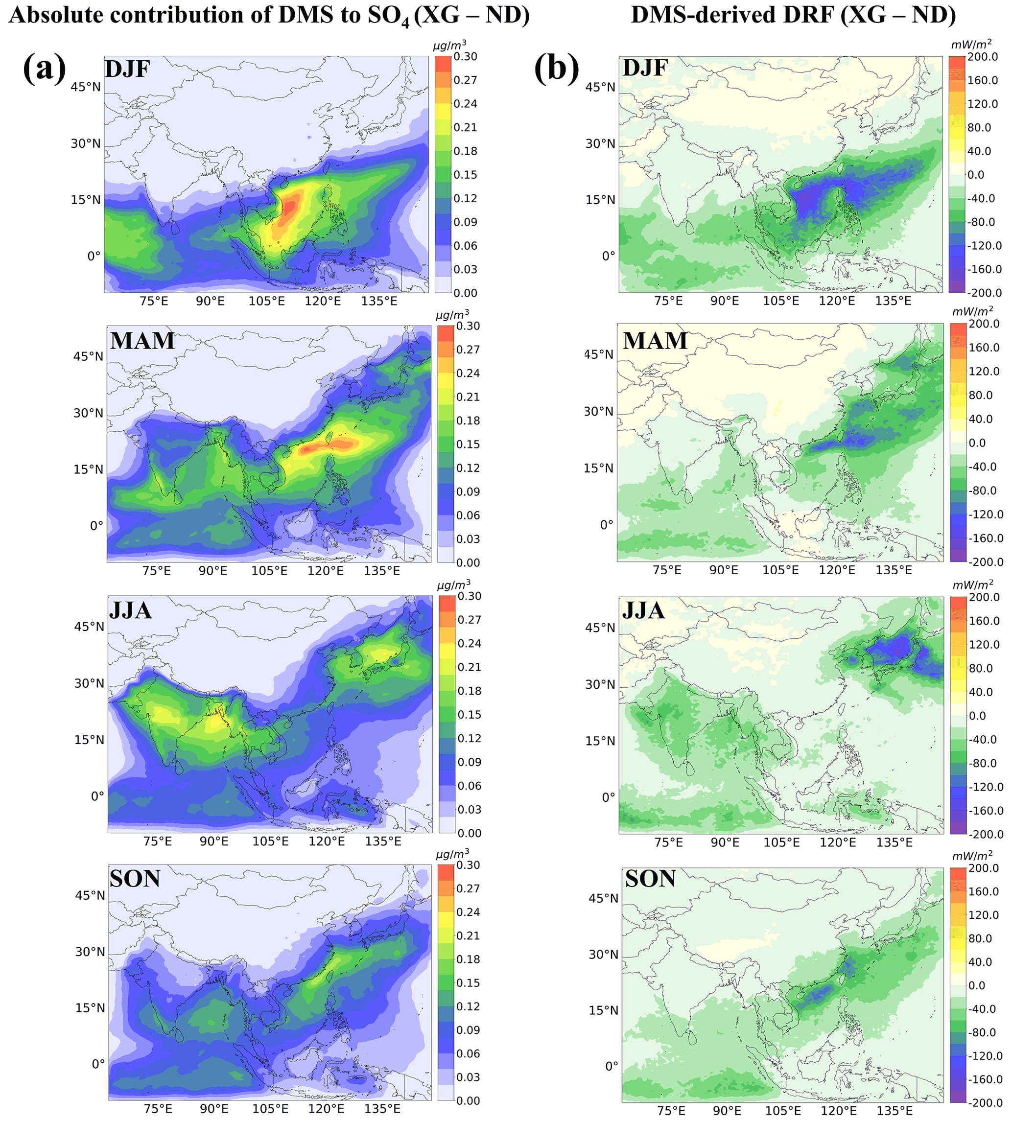
Figure 6 Spatial pattern of the seasonal mean absolute changes in surface ${{\mathrm{SO}}_{\mathrm{4}}}^{\mathrm{2}-}$ (first column) and all-sky DRF (second column) between the XG and ND (no DMS) simulations.

3.3 Seasonal variations of DMS impacts to ${{\mathrm{SO}}_{\mathrm{4}}}^{\mathrm{2}-}$, CCN, and radiative forcing

By updating the DMS emissions in GEOS-Chem (XG-ND), we find an enhancement of near-surface ${{\mathrm{SO}}_{\mathrm{4}}}^{\mathrm{2}-}$ concentrations of 0.1–0.3 µg m⁻³ over most areas of seawater (Fig. 6a). The highest impacts (approximately 0.3 µg m⁻³) occurred in MAM around the South China Sea area due to the highest regional mean DMS concentrations in MAM. However, the spatial distributions of ${{\mathrm{SO}}_{\mathrm{4}}}^{\mathrm{2}-}$ concentrations enhanced by addition of DMS emissions in the four seasons did not exactly follow the spatial and temporal patterns of seawater DMS concentrations (Fig. 2). Sea surface wind speed has noticeable impacts on the sea–air DMS flux and followed atmospheric DMS concentrations, which caused higher atmospheric DMS concentrations over the Indian Ocean in MAM. Ambient oxidant level also plays an important role in the subsequent DMS oxidation phase. For example, higher atmospheric DMS (300–400 pptv) and SO₂ (0.2–0.3 µg m⁻³) concentrations contributed by DMS can be found around the areas of the East China Sea (Figs. S7 and S8) in MAM and JJA. However, a higher contribution of DMS emissions to near-surface ${{\mathrm{SO}}_{\mathrm{4}}}^{\mathrm{2}-}$ concentrations occurred over the South China Sea in DJF and MAM. The spatial disparities might be due to the roles of oxidants in the conversion of SO₂ into ${{\mathrm{SO}}_{\mathrm{4}}}^{\mathrm{2}-}$ in different seasons. Additionally, cloud cover could also affect aqueous conversion.

The magnitude of the all-sky sulfate DRF at the TOA contributed by DMS ranged from −200 to −20 mW m⁻² in four seasons (Fig. 6b). The spatial patterns of DRF are highly consistent with those of ${{\mathrm{SO}}_{\mathrm{4}}}^{\mathrm{2}-}$ concentrations, with the stronger negative DRF (−200 to −120 mW m⁻²) in the areas with higher ${{\mathrm{SO}}_{\mathrm{4}}}^{\mathrm{2}-}$ concentrations contributed by DMS such as the South China Sea, Philippine Sea, and Japan Sea. It should be noted that DRF calculation is from the whole column of the atmosphere, whereas Fig. 6a just shows the surface layer concentrations, yet the spatial results are still qualitatively similar. As reported by some previous studies (Khan et al., 2016; Chen et al., 2018; Zhao et al., 2021), DMS mainly exists in the lower atmosphere, and the impacts of DMS on SO₂ and ${{\mathrm{SO}}_{\mathrm{4}}}^{\mathrm{2}-}$ concentrations are limited to the lower troposphere. So, the magnitude of sulfate DRF at the TOA shown in Fig. 6b is mostly caused by lower-altitude ${{\mathrm{SO}}_{\mathrm{4}}}^{\mathrm{2}-}$ from DMS. ${{\mathrm{SO}}_{\mathrm{4}}}^{\mathrm{2}-}$ aerosols are non-absorbing aerosols that primarily scatter incoming radiation and the increase in reflected solar radiation flux at TOA and almost equally reduce the radiation at the surface (Ramanathan et al., 2001). Thus, for sulfate aerosol, the magnitude of the cooling effect can be estimated from the aerosol radiative forcing at the TOA. The seasonal mean sulfate DRF has contributions of −22.24, −18.79, −21.58, and −17.43 mW m⁻² from DMS over the simulation domain in DJF, MAM, JJA, and SON, respectively. The magnitude of the DMS-induced sulfate DRF in DJF and JJA is higher than other seasons, but the highest impacts of DMS emissions on ${{\mathrm{SO}}_{\mathrm{4}}}^{\mathrm{2}-}$ concentrations occurred in MAM followed by DJF. The all-sky DRF was calculated based on the RRTMG model using aerosol mass concentrations (whole column) and optical parameters along with surface albedo and cloud fractions from MERRA-2-assimilated meteorological data. Hence, aerosol mass concentrations as well as other parameters can impact the magnitude and spatial distributions of the DRF. For clear-sky conditions, aerosol scatters more incoming solar radiation than in all-sky conditions, which leads to aerosol DRF at the TOA and surface increases compared with all-sky conditions.

Figure 7a shows the changes in seasonal mean CCN surface concentrations at 0.2 % supersaturation (CCN 0.2 %) between the XG and ND simulations. Updating the DMS emissions led to an increase in CCN concentrations by 3–42 cm⁻³ over most areas of seawater and an increase of 6–16 cm⁻³ in some coastal regions. The highest increases occurred in DJF, followed by MAM. The impacts of DMS on CCN concentrations are shown in Fig. 6a. The modeled DMS-induced cloud-albedo IRF ranged from −900 to −100 mW m⁻² in the four seasons (Fig. 7b), which is much higher relative to that of the sulfate DRF attributable to DMS. The seasonal mean sulfate IRF had contributions of −43.29, −45.04, −43.60, and −33.03 mW m⁻² from DMS in our domain in DJF, MAM, JJA, and SON, respectively. There are some similarities in the spatial distribution of the effects of DMS on IRF and CCN. However, the strong negative IRF was mainly over remote oceans (−900 to −600 mW m⁻²), while the higher contributions to CCN were concentrated within coastal waters. One explanation for these differences was that strong anthropogenic emissions in Asia led to intense competition for water vapor during cloud-droplet activation, which further decreases the maximum supersaturation achieved in updrafts and limits droplet activation (Kodros et al., 2016). Also, the clouds are not necessarily at a height where CCN changes are affected by DMS.

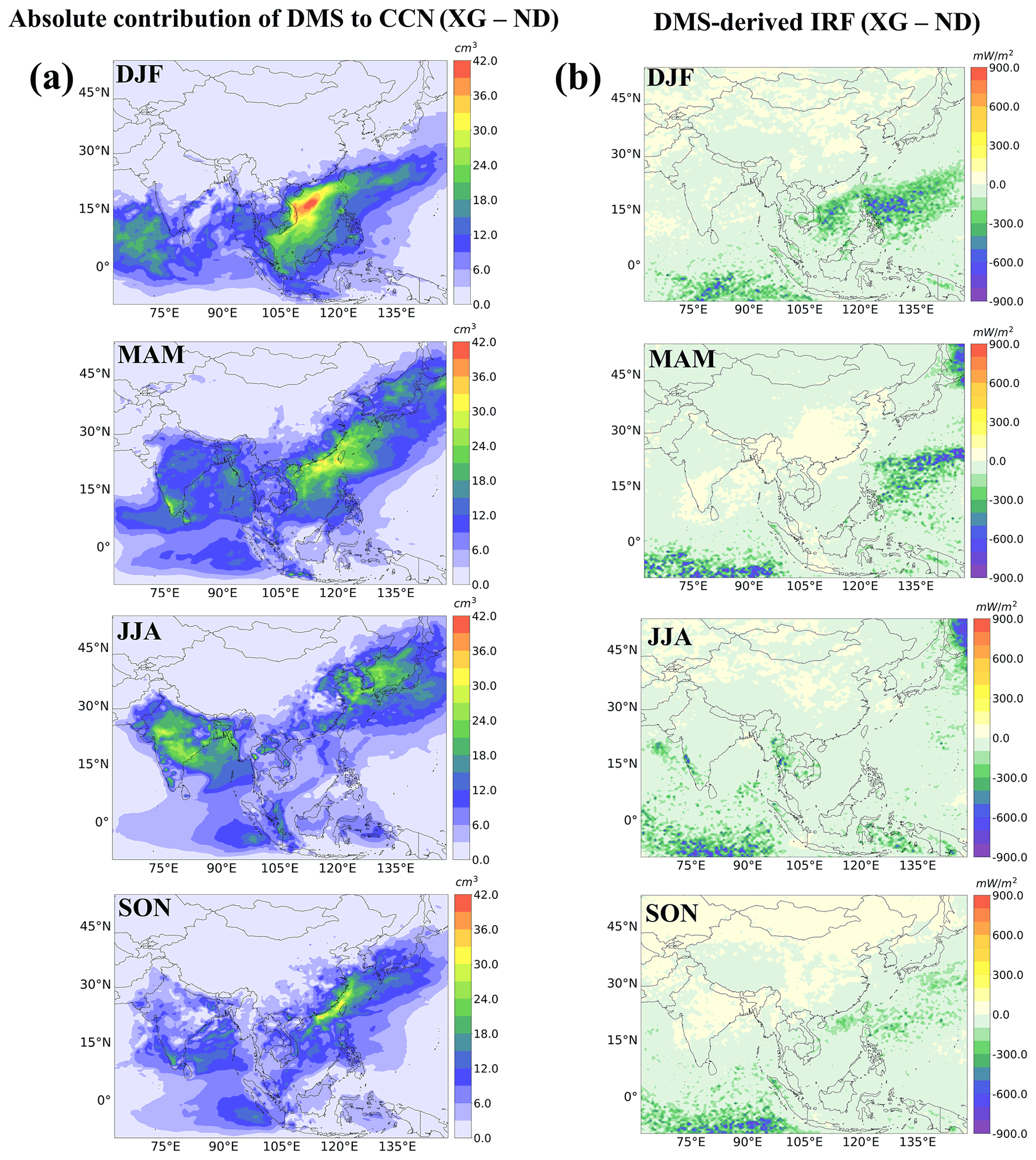
Figure 7 Spatial pattern of the seasonal mean absolute changes in surface CCN (0.2 %) (first column) and cloud-albedo IRF (second column) between the XG and ND (no DMS) simulations.

3.4 Annual DMS impacts on ${{\mathrm{SO}}_{\mathrm{4}}}^{\mathrm{2}-}$, CCN, and radiative forcing

3.4.1 Annual DMS impacts on ${{\mathrm{SO}}_{\mathrm{4}}}^{\mathrm{2}-}$, CCN, and radiative forcing between XG and ND simulation

Figure 8a shows the annual-mean percent changes and absolute changes in ${{\mathrm{SO}}_{\mathrm{4}}}^{\mathrm{2}-}$ and CCN between the XG and ND simulations. Oceanic DMS emissions increased the near-surface ${{\mathrm{SO}}_{\mathrm{4}}}^{\mathrm{2}-}$ and CCN concentrations by 0.1–0.3 µg m⁻³ and 3–42 cm⁻³ over most areas of seawater across the four seasons. Due to heavy amounts of anthropogenic pollutants from the continent, DMS contributed 88 % of ${{\mathrm{SO}}_{\mathrm{4}}}^{\mathrm{2}-}$ and 42 % of CCN in remote oceanic areas. More than 40 % of the ${{\mathrm{SO}}_{\mathrm{4}}}^{\mathrm{2}-}$ and 20 % of the CCN contributed by DMS emissions were also found in the Philippine Sea and Indian Ocean, respectively. DMS had a moderate impact of 0.1–0.18 µg m⁻³ for ${{\mathrm{SO}}_{\mathrm{4}}}^{\mathrm{2}-}$ and 10–22 cm⁻³ for CCN when considering all coastal regions of the simulation domain. Yang et al. (2017) indicated that DMS emissions only have 20 %–40 % of contributions to ${{\mathrm{SO}}_{\mathrm{4}}}^{\mathrm{2}-}$ concentrations over downwind ocean areas of East Asia, which was much lower than the 40 %–70 % contribution estimated in this study. This discrepancy is mainly ascribed to a significant reduction (62 %) in SO₂ emissions in China from 2010 to 2017 (Zheng et al., 2018).

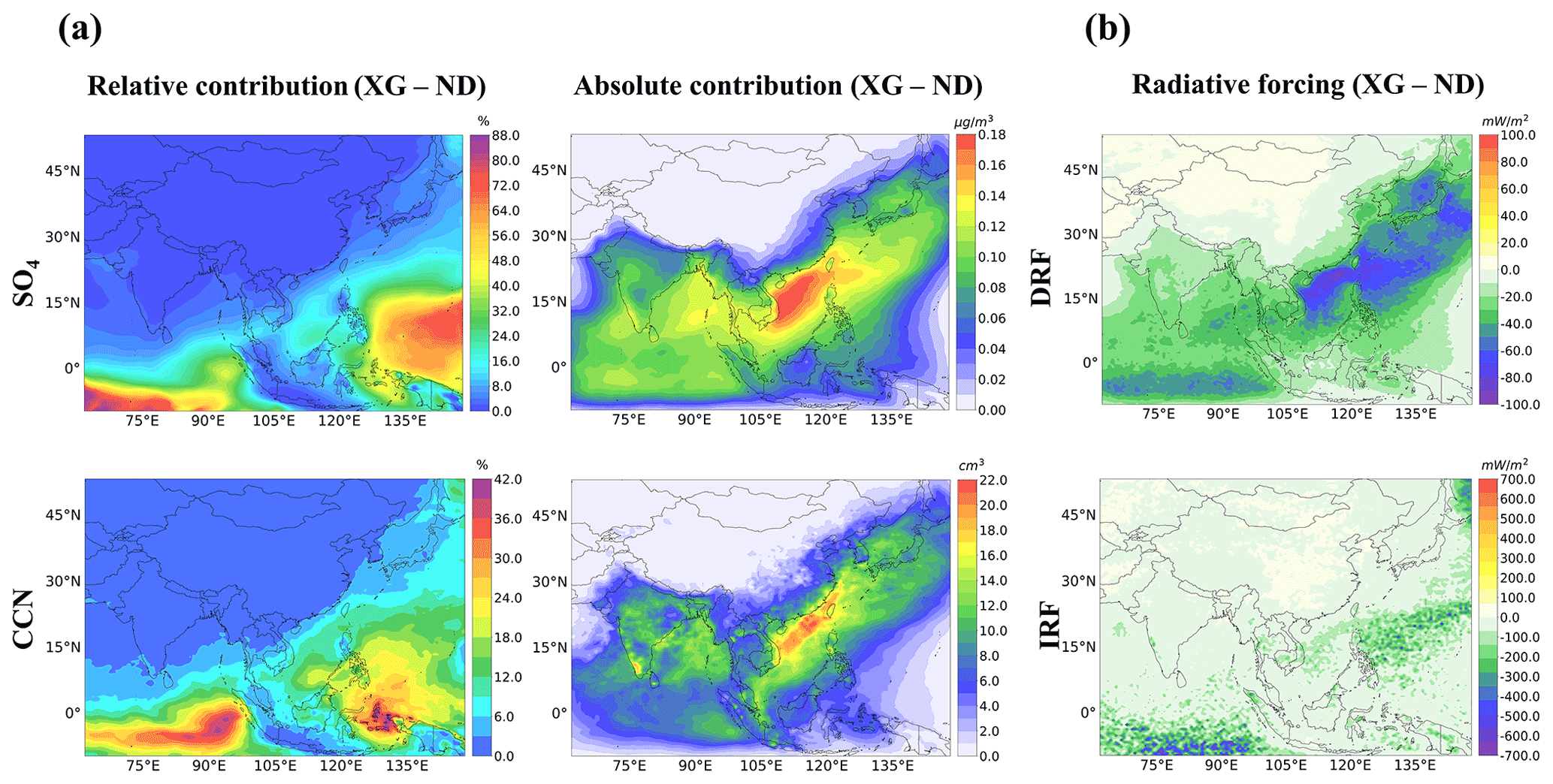
Figure 8 Panel (a) presents the spatial distributions of annual mean percent changes and absolute changes in surface ${{\mathrm{SO}}_{\mathrm{4}}}^{\mathrm{2}-}$ and CCN, and panel (b) presents the spatial distributions of annual mean all-sky DRF and cloud-albedo IRF between XG and ND (no DMS) simulations.

The modeled all-sky DRF of DMS-induced sulfate here ranges from −100 to −10 mW m⁻² (Fig. 8b). The sulfate DRF was strongest (−100 to −60 mW m⁻²) over the South China Sea, which is consistent with the distributions of ${{\mathrm{SO}}_{\mathrm{4}}}^{\mathrm{2}-}$ concentrations contributed by DMS emissions. The DMS-induced cloud-albedo IRF (−700 to −100 mW m⁻²) here was higher than the all-sky DRF estimate. A relatively strong cooling IRF (−700 to −400 mW m⁻²) induced by DMS emissions can be seen in the vicinity of the equatorial belt in the Indian Ocean and northwestern Pacific Ocean. The simulated annual mean sulfate DRF and IRF are −20.01 and −41.26 mW m⁻² over the simulation domain, respectively. Li et al. (2019) estimated the annual mean all-sky DRF of −100 mW m⁻² from DMS emissions over the East China Sea. Our estimates (−20.01 mW m⁻²) were lower than their result, which is likely attributable to discrepancies in the DMS emissions used to drive the model.

3.4.2 Annual DMS impacts on ${{\mathrm{SO}}_{\mathrm{4}}}^{\mathrm{2}-}$, CCN, and radiative forcing between XG and LANA simulations

To quantify the impacts of DMS emissions changes on ${{\mathrm{SO}}_{\mathrm{4}}}^{\mathrm{2}-}$, CCN, and radiative forcing, we compared the XG and LANA simulations (Fig. S9a). Increases in ${{\mathrm{SO}}_{\mathrm{4}}}^{\mathrm{2}-}$ and CCN can be found in the areas of Indonesia and the northwestern Pacific Ocean (Fig. S9a), which was generally consistent with the changes in DMS emissions fluxes between XG and LANA (Fig. 3b). DMS emissions changes (between XG and LANA) accounted for 4 %–20 % and 6 %–18 % of ${{\mathrm{SO}}_{\mathrm{4}}}^{\mathrm{2}-}$ and CCN concentrations over areas of Indonesia and 2 %–10 % and 3 %–6 % of those concentrations over the northwestern Pacific Ocean, respectively. The largest decreases were seen in the vicinity of the Indian Ocean, which was −0.06 µg m⁻³ for ${{\mathrm{SO}}_{\mathrm{4}}}^{\mathrm{2}-}$ and −10 cm⁻³ for CCN. Due to the higher background concentrations contributed by anthropogenic sources, the relative percent change was smaller over that area, where DMS emissions changes only accounted for −8 % to −4 % for ${{\mathrm{SO}}_{\mathrm{4}}}^{\mathrm{2}-}$ and −6 % to −3 % for CCN. Also, changes in DMS fluxes around the equatorial belt in the western Pacific Ocean (Fig. 3b) did not directly link to negative changes in ${{\mathrm{SO}}_{\mathrm{4}}}^{\mathrm{2}-}$ and CCN, which was most likely offset by large-scale transport of sulfate caused by DMS from the East China Sea. The changes in annual mean DRF and IRF from XG–LANA simulation are shown in Fig. S9b. Decreases in DRF (−20 to −5 mW m⁻²) mainly were concentrated over the northwestern Pacific Ocean. The largest increase in DRF (up to 40 mW m⁻²) was found in the areas of the Japan Sea, and most of the increases in DRF (5 to 20 mW m⁻²) were mainly distributed in the region of the Indian Ocean and land areas of India. Their spatial patterns were consistent with distributions of absolute changes in ${{\mathrm{SO}}_{\mathrm{4}}}^{\mathrm{2}-}$ concentrations. The largest changes in IRF were found in areas of the northwestern Pacific Ocean and the Sea of Okhotsk, with changes of up to −200 and 200 mW m⁻². The decreases in IRF from the XG–LANA simulation can span most of the Pacific Ocean over the simulation domain and some continental regions, and increases in IRF are more concentrated within the Indian Ocean and Sea of Okhotsk. Generally, our estimated sea–air DMS fluxes are lower than those from Lana et al. (2011) over most of the ocean areas, but the DMS-caused changes to ${{\mathrm{SO}}_{\mathrm{4}}}^{\mathrm{2}-}$, CCN, and radiative forcing were more varied, with the increases over the northwestern Pacific Ocean for ${{\mathrm{SO}}_{\mathrm{4}}}^{\mathrm{2}-}$ and CCN,and decreases in the regions of Indian Ocean or increases in the regions of the Indian Ocean for DRF and IRF and decreases over the northwestern Pacific Ocean.

3.5 Limitations of this study

We found several limitations in our emission estimates and modeling study. We try to use machine learning estimates of DMS concentrations to fill the regions without observations. While the recently measured 1022 seawater DMS observations over Chinese seas included a training period, for some months (January, November, etc.) there were still not enough data to create a monthly mean. Hence, we temporally averaged input parameters to a seasonal period rather than use monthly data, which is a limitation of this study, but as shown in Sect. 3.1, the estimated results showed distinct seasonal variations, and the results are comparable with other studies. Due to the limited continuous measurements of atmospheric DMS and MSA concentrations, we only presented all the averaged cruise survey observations for DMS model evaluation and temporal variation of MSA prediction performance evaluated only from a single observation site. We acknowledge that this is an important limitation of this study, which prevents us from giving comprehensive estimates (on temporal and spatial scales) of the advantage of our updated DMS emissions. More marine and atmospheric observational data are necessary for further model evaluation.

In addition, due to the limited high-temporal-resolution monitoring data of CCN for the simulation year 2017 in our domain, we verified the model performance of the CCN simulation by comparing the modeled results with the collected mean annual observed concentrations of CCN in other previous studies and satellite-retrieved CCN concentrations. We acknowledge that the CCN model–measurement comparisons listed in Table S5 are not the exact times where simulated and satellite-retrieved CCN (given the uncertainty in water uptake and size distributions) are not necessarily accurate enough to represent true atmospheric CCN concentrations in 2017.

Modeled AOD may be biased during cloudy conditions when AERONET measurements cannot be made. Hence, there would be an uncertainty in using monthly averaged measurements and model predictions for comparison (Schutgens et al., 2016).

Different chemical mechanisms of various chemical-transport models and the treatment of aerosol optical properties can also lead to differences in simulation results. Globally, the annual-mean DRF and IRF contributed by DMS reported by other studies (as listed in Table S6) varied from −0.23 to −0.074 W m⁻² and from −6.55 to −0.3 W m⁻², respectively. Aerosol–cloud interactions are a major source of uncertainty in the prediction of climate change, impacting radiative forcing estimates, especially the IRF calculation. Differences in aerosol nucleation schemes, activation parameterizations, and emissions between models can contribute to large discrepancies in their simulation results (Carslaw et al., 2013). However, we did not explore the impact of different nucleation schemes on radiative forcing. We recommend that this should be done in future work to minimize uncertainties in future modeling studies.

4 Conclusions

In this study, we utilized the XGBoost machine learning algorithm to estimate seawater DMS concentrations by training 12 ocean environmental parameters on newly updated DMS measurements; 1022 recent seawater DMS measurements over Chinese seas were included in our training data, and we used the machine learning method to fill the gap at times and in locations without observations. The DMS model–measurement validation results showed that our XGBoost estimates could capture the observed DMS concentrations with a correlation coefficient of 0.75. Zonal mean DMS concentrations between 10^∘ S and 30^∘ N latitude areas of simulation domain were higher in MAM than in JJA, and most of the ocean area was concentrated in the 10^∘ S and 30^∘ N latitude band, which led to the highest regional mean DMS concentrations observed in MAM. We estimated annual DMS emission fluxes of 1.25 Tg (S), which accounted for 15.4 % of anthropogenic sulfur emissions over the entire simulation domain (covering most of Asia) in 2017. Comparative analysis revealed that the sea–air DMS flux estimated in this study (from XG estimates) was generally lower than those from global-database DMS emissions (Lana et al., 2011). The model estimates of DMS and MSA from XG simulation were evaluated by comparing them with cruise survey experiments and long-term online measurement site data. In general, the improvement in model performance can be observed by comparing XG with the LANA simulation, which uses the global-database DMS emissions.

The modeled DMS-induced sulfate DRF and IRF ranged from −200 to −20 mW m⁻² and from −900 to −100 mW m⁻² across the four seasons, respectively. The stronger negative DRF (−120 to −200 mW m⁻²) was in the areas with higher ${{\mathrm{SO}}_{\mathrm{4}}}^{\mathrm{2}-}$ concentrations contributed by DMS, such as the South China Sea, Philippine Sea, and Japan Sea. However, the strong negative IRF was mainly over remote oceans (−900 to −600 mW m⁻²), which did not match with the spatial distributions of contributions of DMS to CCN concentrations due to the role of clouds in the IRF. Annually, DMS-induced sulfate IRF (−700 to −100 mW m⁻²) here was obviously higher than those all-sky DRF (−100 to −10 mW m⁻²). By adding our updated DMS emissions to a simulation with no DMS (XG–ND), we predict the enhancement of near-surface ${{\mathrm{SO}}_{\mathrm{4}}}^{\mathrm{2}-}$ and CCN concentrations by 0.1–0.3 µg m⁻³ and 3–42 cm⁻³, respectively, over most oceanic areas in all four seasons. We found higher contributions from DMS emissions to ${{\mathrm{SO}}_{\mathrm{4}}}^{\mathrm{2}-}$ and CCN in MAM and DJF than JJA and SON.

In this work, we quantified the contributions of DMS to atmospheric ${{\mathrm{SO}}_{\mathrm{4}}}^{\mathrm{2}-}$ and CCN aerosol concentrations along with their radiative effect over a modeled Asian domain (covering most of Asia). This work provides better insights into the source strength of DMS and its impact on climate, addressing knowledge gaps related to factors controlling aerosols in the marine boundary layer and their climate impacts. As discussed in Sect. 3.6, there are several limitations that need to be improved upon in future work. More marine and atmospheric observational data are necessary for further DMS emission estimates and model evaluation to explore the interactions of DMS with aerosols and radiative forcing. In future work, we also need to explore the impact of different aerosol nucleation schemes on radiative forcing to more completely quantify the uncertainties in our modeling study.